Separation of Moving Sound Sources Using Multichannel NMF and Acoustic Tracking

Abstract

In this paper we propose a method for separation of moving sound sources. The method is based on first tracking the sources and then estimation of source spectrograms using multichannel non-negative matrix factorization (NMF) and extracting the sources from the mixture by single-channel Wiener filtering. We propose a novel multichannel NMF model with time-varying mixing of the sources denoted by spatial covariance matrices (SCM) and provide update equations for optimizing model parameters minimizing squared Frobenius norm. The SCMs of the model are obtained based on estimated directions of arrival of tracked sources at each time frame. The evaluation is based on established objective separation criteria and using real recordings of two and three simultaneous moving sound sources. The compared methods include conventional beamforming and ideal ratio mask separation. The proposed method is shown to exceed the separation quality of other evaluated blind approaches according to all measured quantities. Additionally, we evaluate the method’s susceptibility towards tracking errors by comparing the separation quality achieved using annotated ground truth source trajectories.

I Introduction

Separation of sound sources with time-varying mixing properties, caused by the movement of the sources, is a relevant research problem for enabling intelligent audio applications in realistic operation conditions. These applications include, for example, speech enhancement and separation for automatic speech recognition [1] especially when using voice commanded smart devices from afar [2]. Another emerging application field includes immersive audio for augmented reality [3] which requires modification of the observed sound scene for example by removing sound sources and replacing them with augmented content. Separation of non-speech sources can be also used to improve sound event detection in multi-source noisy environment [4]. Most existing works related to sound separation are assuming stationary sources, and not many blind methods have targeted the problem of moving sound sources despite its high relevance in realistic conditions.

The problem of sound source separation either from single or multi-channel recordings has been tackled with various methods over the years. The methods maximizing statistical independence of non-Gaussian sources, such as the independent component analysis (ICA) have been used for unmixing the sources in frequency domain [5, 6]. The concept of binary clustering of time-frequency blocks based on inter-channel cues, namely the level and the time difference, has resulted into class of separation methods based on time-frequency masking [7, 8]. Use of binary masks requires assuming that sound sources occupy disjoint time-frequency blocks [9]. More recently, single-channel speech enhancement and separation has been performed with the aid of machine learning and specifically by using deep neural networks (DNNs) [10, 11] for predicting the time-frequency masks for separation. Combining prediction of source spectrogram using DNNs and spatial information in the form of source covariance matrices for audio source separation has been proposed in [12, 13].

Another machine learning tool for masking based source separation is the spectrogram factorization by non-negative matrix factorization (NMF) and non-negative matrix deconvolution (NMD) which both have been widely utilized for speech separation and enhancement [14, 15]. The NMF model decomposes mixture magnitude spectrogram into spectral templates and their time-dependent activations. In the case of single channel mixtures the separation is achieved by learning of noise or speaker dependent spectral templates from isolated sources in a training stage.

The NMF model can be extended for multichannel mixtures by incorporating spatial covariance matrix (SCM) estimation for the NMF components as in [16, 17, 18, 19, 20]. The analysis and introduction of spatial properties for NMF components allows separation based on spatial information, i.e., NMF components with similar spatial properties are considered to originate from the same sound source. These models require operation with complex-valued data and hereafter we refer to these extensions as multichannel NMF.

Recording of a realistic auditory scene often consists of sound sources which are moving with respect to the recording device, and conventional separation approaches assuming time-invariant mixing are not suitable for such a task. However, moving sound sources can be considered stationary within a short time block where the mixing can be assumed to be time-invariant. Using the block-wise approach for separation of moving sound sources requires merging the separated sources across individually processed blocks. For example, in block-wise ICA [21, 22, 23] this is done by propagating the mixing matrix from the previous block and thus slowly adapting the mixing and preserving the source ordering in consecutive blocks. A recent generalization of multichannel NMF model [16] for time-varying mixing and separation of moving sound sources was proposed in [24]. The reported results are promising, however the proposed algorithm requires using other state-of-the art source separation method in a blind setting for initialization.

Alternatively, separation of moving sources can be achieved by tracking the spatial position or direction of arrival (DOA) of the sources and using spatial filtering (beamforming or separation mask) for extracting the signal originating from the estimated position or direction in each time instance. In [25] the problem of DOA tracking and separation mask estimation is formulated jointly, however in this paper we consider a two stage approach where the acoustic tracking is done first and the separation masks are estimated in a separate (offline) stage. Also the separation masks are binary in [25] which will lead to compromised subjective separation quality even if oracle masks are used.

Acoustic localization with microphone arrays can be achieved by transforming the time-difference of arrival (TDOA) obtained using generalized cross-correlation (GCC) into source position estimates [26]. Methods for estimation of trajectories of moving sound sources are based on Kalman filtering and its non-linear extensions [27, 28] for estimating the underlying state (position of the sound source) from the TDOA measurements. Alternatively, sequential Monte Carlo methods, i.e., particle filtering [29, 30] have been applied for tracking the position of the source based on TDOA measurements. For even more difficult case of multiple target tracking with data association problem, a Rao-Blackwellised particle filtering (RBPF) was proposed in [31, 32] and applied for acoustic tracking of multiple speakers in [33]. Additionally, the use of directional statistics and quantities wrapped on a unit circle or a sphere, such as the interchannel phase difference, has been recently considered for speaker tracking [34, 35].

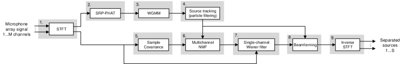
Figure 1: The block diagram of the proposed processing consisting of source tracking and multichannel NMF for separation of detected and tracked sound sources.

In this paper we propose a separation method for moving sound sources based on acoustic tracking and estimation of source spectrogram from the tracked directions using the multichannel NMF with time-varying SCM model. The main contributions of this paper include: formulation of multichannel NMF model for time-varying mixing (moving sound sources), integration of the spatial model with acoustic tracking to define spatial properties of sources in form of SCMs in each time frame and finally presenting the update equations for optimizing the multichannel NMF model parameters minimizing squared Frobenius norm. The parametrization of source DOA with directional statistics and using the tracker uncertainty for defining the SCMs of sources is a novel approach for representing the spatial location and spread of sound sources in the multichannel NMF. The acoustic tracker realization is combination of existing works on wrapped Gaussian mixture models [36] and particle filtering [37], but it will be presented in detail due to its output statistics are utilized in the proposed time-varying SCM model.

The evaluation of the proposed separation algorithm is based on objective separation criteria [38, 39, 40] and testing with mixtures of two and three simultaneous moving speakers. Additionally, hand-annotated source DOA trajectories are used for evaluating the performance of the acoustic tracker realization and studying the susceptibility of the proposed separation algorithm towards tracking errors. The compared separation methods include conventional beamforming (DSB and MVDR) and upper reference is obtained by ideal ratio mask (IRM) separation [41]. The proposed method achieves superior separation performance and the use of annotated trajectories shows no significant increase in separation performance, proving the proposed method suitable for realistic operation in a blind setting.

The paper is organized as follows. First the problem of separating moving sound sources and an overview of the proposed processing is given in Section II. Next we introduce directional statistics and describe the acoustic source tracker realization in Section III. In Section IV the multichannel NMF separation model for sources with time-varying mixing is proposed and the utilization of tracker output within the separation model is explained. In Section V the tracking and separation performance of the proposed algorithm is evaluated using real recorded test material captured using a compact four-element microphone array. The work is concluded in Section VII.

II Problem statement and algorithm overview

II-A Mixing model of moving sound sources

A microphone array composed of microphones $(m=1,\dots,M)$ observes a mixture of $p=1,\dots,P$ source signals ${s}_{p}(t)$ sampled at discrete time instances indexed by $t$. The sources are moving and have time-varying mixing properties, denoted by room impulse response (RIR) ${h}_{pmt}(\tau)$, for each time index $t$. The resulting mixture signal can be given as

$${x}_{m}(t)=\sum_{p=1}^{P}\sum_{\tau}{s}_{p}(t-\tau){h}_{pmt}(\tau).$$ (1)

In sound source separation the aim is to estimate the source signals ${s}_{p}$ and their mixing ${h}_{pmt}(\tau)$ by only observing ${x}_{m}(t)$.

In this paper audio is processed in frequency domain obtained using the short time Fourier transform (STFT). The STFT of a time-domain mixture signal is calculated by dividing the signal into short overlapping frames, applying a window function and taking the discrete Fourier transform (DFT) of the windowed frame. The mixing properties denoted by the time-dependent RIRs ${h}_{pmt}(\tau)$ change slowly over time and in practice the difference between adjacent time indices $t$ is small, thus we can consider mixing being constant within a small time window. This allows to approximate the time-dependent mixing (1) in time-frequency (TF) domain as

$$\mathbf{x}_{fn}\approx\sum_{p=1}^{P}\mathbf{h}_{fn,p}s_{fn,p}=\sum_{p=1}^{P}\mathbf{{y}}_{fn,p}.$$ (2)

The STFT of the mixture signal is denoted by $\mathbf{x}_{fn}=[x_{fn1},\dots,x_{fnM}]^{T}$ for each TF-point $(f,n)$ of each input channel $(m=1,\dots,M)$. The single-channel STFT of each source $p$ is denoted by $s_{fn,p}$ and their frequency domain RIRs (fixed withing each time frame $n$) are denoted by $\mathbf{h}_{fn,p}=[h_{fn1},\dots,h_{fnM}]^{T}$. The source signals convolved with the impulse responses are denoted by $\mathbf{{y}}_{fn,p}$.

II-B Overview of the processing

The proposed method consists of source spectrogram estimation based on the DOA of the sources of interest in each time frame and the estimated spectrograms are used for separation mask generation by generalized Wiener filter. The processing is based on two stages: the acoustic tracker and the offline separation mask estimation by multichannel NMF. The block diagram of the method is illustrated in Figure 1. The source tracking branch operates frame-by-frame and can be though as online algorithm while the parameters of the multichannel NMF model are estimated from the entire signal at once (offline).

First the STFT of the input signals is calculated. The tracking branch starts with calculating the steered response power (SRP) of the signal under analysis. SRP denotes the spatial energy as a function of DOA for each time frame. A wrapped Gaussian mixture model (WGMM) [36] of the SRP function in each time frame is estimated, which converts spatial energy histogram (i.e. the SRP) into DOA measurements. WGMM parameters are used as measurements in acoustic tracking which is implemented using particle filtering [37]. The multi-target tracker detects the births and deaths of sources, solves the data-associations of measurement belonging to one of existing sources and predicts the source trajectories.

In the second stage a spatial covariance matrix model (SCM model) [19] parameterized by DOA is defined based on the acoustic tracker output (source DOA at each time-frame). The obtained SCMs denote the spatial behavior of sources over time and a spectral model of sources originating from the tracked direction is estimated using multichannel NMF. The multichannel source signals are reconstructed using a single-channel Wiener filter based on the estimated spectrogram of each source and single-channel signals are obtained by applying the delay-and-sum beamforming to the separated multichannel signals. Finally, time-domain signals are reconstructed by applying inverse STFT and overlap-add.

III Source trajectory estimation

The goal of the first part of the proposed algorithm is to estimate DOA trajectories of the sound sources that are to be separated. The process consist of three consecutive steps: calculating the spatial energy emitted from all directions (Section III-A), converting the discrete spatial distribution into DOA measurements (Sections III-B and III-C) and multi-target tracking consisting of source detection, data-association and source trajectory estimation (Section III-D).

III-A Time-difference of arrival and steered response power

Spatial signal processing with spaced microphone arrays is based on observing time delays between the array elements. In far-field propagation the wavefront direction of arrival corresponds to a set of TDOA values between each microphone pair. We start by defining a unit direction vector $\mathbf{k}\in\mathcal{R}^{3},||\mathbf{k}||=1$ originating from the geometric center of the array $\mathbf{p}=[0,0,0]^{T}$ and pointing towards direction parametrized by azimuth $\theta\in[0,2\pi]$ and elevation $\varphi\in[0,\pi]$. Given a microphone array consisting of two microphones $m_{1}$ and $m_{2}$ at locations $\mathbf{m}_{1}\in\mathcal{R}^{3}$, $\mathbf{m}_{2}\in\mathcal{R}^{3}$ the TDOA between them for a sound source at direction $\mathbf{k}$ is obtained as

$$\tau(m_{1},m_{2})=\frac{-\mathbf{k}^{T}(\mathbf{m}_{1}-\mathbf{m}_{2})}{v},$$ (3)

where $v$ is the speed of sound. The above TDOA corresponds to a phase difference of $\exp(-j\omega_{f}\tau(m_{1},m_{2}))$ in the frequency domain, where $\omega_{f}=2\pi(f-1)F_{s}/{N}$ ($F_{s}$ is the sampling frequency and $N$ is the STFT window length).

From now on we operate with a set of different directions indexed by $d=1,\dots,D$ and the direction vector corresponding to $d$th direction is defined as $\mathbf{k}_{d}$ resulting to TDOA of $\tau_{d}(m_{1},m_{2})$. The spatial energy originating from the direction $[\theta_{d},\varphi_{d}]$ at each time frame $n$ can be calculated using the steered response power (SRP) with PHAT weighting [42] defined as

$$S_{dn}=\sum_{m_{1}=1}^{M-1}\sum_{m_{2}=m_{1}+1}^{M}\sum_{f=1}^{F}\frac{x_{fnm_{1}}x_{fnm_{2}}^{*}}{|x_{fnm_{1}}x_{fnm_{2}}^{*}|}\exp(j\omega_{f}\tau_{d}(m_{1},m_{2})),$$ (4)

where ^∗ denotes complex-conjugate and the term $\exp(j\omega_{f}\tau_{d}(m_{1},m_{2}))$ is responsible for time-aligning the microphone signals. SRP denotes the spatial distribution of the mixture consisting of spatial evidence from multiple sources and searching for multiple local maxima of the SRP function at a single time frame $n$ corresponds to DOA estimation of sources present in that time frame. Repeating the pick peaking for all time frames of SRP would result to DOA measurements that are permuted over time and subsequently in the tracking stage the permuted DOA measurements are associated to multiple sources over time.

In a general case the directions $d=1,\dots,D$ would uniformly sample a unit sphere around the array, but in this paper we only consider the zero elevation plane, i.e., $\varphi_{d}=0\;\forall d$. We assume that the sources of interest lie approximately on the xy-plane with respect to the microphone array and the directional statistics used in tracking of the sources simplifies to a univariate case. A sparse grid of directions vectors with spacing of adjacent azimuths by $\frac{\pi}{12}$ is illustrated in Figure 2 along with the array casing and microphones corresponding to the actual compact array used in the evaluations.

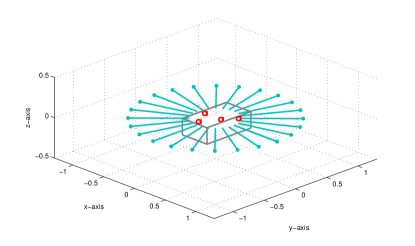
Figure 2: Illustration of a sparse grid of direction vectors by lines with dot in end and an example array enclosure and enclosed microphones (circles).

III-B Wrapped Gaussian mixture model

Instead of searching peaks from the SRP (4), we propose to model the mixture spatial distribution using a wrapped Gaussian mixture model (WGMM) estimated separately for each time-frame of the SRP. The estimation of the parameters of the WGMM results to converting the discrete spatial distribution obtained by SRP into multiple DOA measurements with mean, variance and weight. The individual wrapped Gaussians model the spatial evidence caused by the actual sources while some of them may model the noise or phantom peaks in the SRP caused by sound reflecting from boundaries. The use of WGMM alleviates effect of noise when the width of each peak, denoted by variance of each wrapped Gaussian, can be used to denote measurement uncertainty in the acoustic tracking stage.

The probability density function (PDF) of univariate wrapped Gaussian distribution [36, 43, 44] with mean $\mu$ and variance $\sigma^{2}$ can be defined as

$$P(\theta;\mu,\sigma^{2})= \sum_{l=-\infty}^{\infty}\mathcal{N}(\theta;\mu+l2\pi,\sigma^{2})$$

$$= \sum_{l=-\infty}^{\infty}\frac{1}{\sqrt{2\pi\sigma^{2}}}e^{-\frac{(\theta-\mu+2\pi l)^{2}}{2\sigma^{2}}},$$ (5)

where $\mathcal{N}(\theta;\mu,\sigma^{2})$ is a PDF of a regular Gaussian distribution, $l$ is the wrapping index of $2\pi$ multiples and $\theta\in[-\pi,\pi]$. The multivariate version of the wrapped Gaussian distribution is given in [36], but it is not of interest in this paper.

The WGMM with weights $a_{k}$ for each wrapped Gaussian distribution $k$ is defined as

$$P(\theta;\mathbf{a},\boldsymbol{\mu},\boldsymbol{\sigma}^{2})=\sum_{k=1}^{K}a_{k}\sum_{l=-\infty}^{\infty}\mathcal{N}(\theta;\mu_{k}+l2\pi,\sigma_{k}^{2}).$$ (6)

where $K$ is the total number of wrapped Gaussians in the model and EM algorithm for estimating parameters $\{\mathbf{a},\boldsymbol{\mu},\boldsymbol{\sigma}^{2}\}$ that maximize the log likelihood

$$\log L=\sum_{d=1}^{D}\log\sum_{k=1}^{K}a_{k}\sum_{l=-\infty}^{\infty}\mathcal{N}(\theta_{d};\mu_{k}+l2\pi,\sigma_{k}^{2}),$$ (7)

is given in [36, 44]. The parameter $\theta_{d}$ denotes the azimuth angles of the directions indices $d=1,\dots,D$ used to calculate SRP in Equation (4).

Figure 3: The observed SRP $S_{dn}$ for a single time-frame $n$ and the WGMM with $K=3$ estimated from it.

The EM-algorithm for WGMM as presented in [36, 44] requires observing data points generated by the underlying distribution whereas $S_{dn}$ for a single frame $n$ is effectively a histogram denoting spatial energy emitted from each scanned direction indexed by $d$. Estimating the WGMM parameters based on the histogram requires modification of the algorithm presented in [36, 44] to account for inputs consisting of discretely sampled mixture distribution, i.e., the histogram bin values. The modification results to Algorithm 1 where SRP of a single frame $n$ is denoted by $s_{d}$ and the updates are iterated until converge of $\eta_{dkl}$. Prior knowledge can be used to set initial values for $a_{k},\mu_{k}$ and $\sigma_{k}^{2}$ or they can be initialized randomly. An example of the SRP $S_{dn}$ of a single time-frame and three component WGMM estimated from it is illustrated in Figure 3.

Algorithm 1 EM-algorithm for estimation of WGMM model parameters for a histogram $s_{d}$ (single frame from the entire SRP $S_{dn}$).

0:  Histogram data $s_{d}$ and initial values for $a_{k},\mu_{k}$ and $\sigma_{k}^{2}$

  E-STEP

  $\eta_{dkl}=\frac{\mathcal{N}(\theta_{d};\mu_{k}+l2\pi,\sigma_{k}^{2})a_{k}}{\sum_{k=1}^{K}\sum_{l=-\infty}^{\infty}\mathcal{N}(\theta_{d};\mu_{k}+l2\pi,\sigma_{k}^{2})a_{k}}$

  M-STEP

  $\mu_{k}=\frac{\sum_{d=1}^{D}\sum_{l=-\infty}^{\infty}(\theta_{d}-2\pi l)\eta_{dkl}s_{d}}{\sum_{d=1}^{D}\sum_{l=-\infty}^{\infty}\eta_{dkl}s_{d}}$

  $\sigma_{k}^{2}=\frac{\sum_{d=1}^{D}\sum_{l=-\infty}^{\infty}(\theta_{d}-\mu_{k}-2\pi l)\eta_{dkl}s_{d}}{\sum_{d=1}^{D}\sum_{l=-\infty}^{\infty}\eta_{dkl}s_{d}}$

  $a_{k}=\frac{1}{\sum_{d}s_{d}}\sum_{d=1}^{D}\sum_{l=-\infty}^{\infty}\eta_{dkl}s_{d}$

III-C DOA measurements by WGMM

Algorithm 1 is applied individually for each time frame $n=1,\dots,N$ of $S_{dn}$. A mixture of $k=1,\dots,K$ wrapped Gaussians for each time frame is obtained and the resulting means $\mu_{n,k}$ with variances $\sigma_{n,k}$ and weights $a_{n,k}$ are considered as permuted DOA measurements. At this point of the algorithm it is unknown which of the measurements $k=1,\dots,K$ in each frame $n$ are caused by actual sources and which correspond to noise. Also the detection of sources and association of different measurements $k$ to sources $p$ over time is unknown, i.e. $k$th measurement in adjacent frames may be caused by different sources. The source detection, data-association and actual source trajectory estimation is solved using the Rao-Blackwellized particle filtering introduced in Section III-D.

Random initialization of Algorithm 1 could be used in each time frame. However, initial values close to the optimal ones speed up the algorithm convergence and in practice estimates from previous frame can be used as initialization for the subsequent frame. Please note that this initialization strategy does not guarantee preserving any association between $k$th wrapped Gaussians in adjacent frames and ordering need to be considered as permuted.

The WGMM parameters $\{\mu_{n,k},\sigma_{n,k},a_{n,k}\}$ are hereafter referred to as DOA measurements regarding the acoustic tracking: $\mu_{n,k}$ are the measurement means, $\sigma_{n,k}$ denote measurement reliability and $a_{n,k}$ are the proportional weights of the measurements. Given that a WGMM with $K$ components for each time frame is estimated, not all WGMM components are caused by actual spatial evidence but are merely modeling the noise floor and phantom peaks in the SRP. The situation is illustrated in Figure 3, where the third WGMM component with mean $\mu=71^{\circ}$ has a very high variance $\sigma^{2}=117^{\circ}$ in comparison to the actual observable peaks.

By investigating the variance and weight of each WGMM component the false measurements can be efficiently removed before applying the actual tracking algorithm. The means $\mu_{n,k}$ for each time frame for an arbitrary test signal and after removing measurements with $\sigma_{n,k}>35^{\circ}$ or $a_{n,k}<0.15$ are illustrated in Figure 4. The removal of false measurements reveals two distinct observable trajectories, however the data association between each frame is unknown at this stage. The thresholds for measurement removal can be set to be global (signal and capturing environment independent) and their choice is discussed in more details in Section V.

III-D Acoustic tracking of multiple sound sources

The problem setting in tracking of multiple sound sources is as follows. Multiple DOA measurements are obtained in each time frame and the task is to decide whether the new measurement is 1) associated to an existing source 2) identified as clutter, 3) evidence of new source (birth) and finally 4) determining possible deaths of existing sources. After the data-association step the dynamic state of the active sources is updated and particularly it is required to preserve the source statistics over short inactive segments (pauses between words in speech) by prediction based on previous state of the source (location, velocity and acceleration).

In the following, we shortly review the Rao-Blackwellized particle filter (RBPF) framework proposed in [31] for the problem of multi-target tracking and use its freely available implementation documented in [37]. We give the state-space representation of the dynamical system that is being tracked but we do not go to any further details of RBPF. The algorithm proposed in [31] and the associated implementation has been used in [45] for tracking the azimuth angle of speakers in a similar setting.

Multi-target tracking by RBPF is essentially based on dividing the entire problem into two parts, estimation of data association and tracking of single targets. This can be done with the Rao-Blackwellization procedure [32] where the estimation of the posterior distribution of the data associations is done first and then applying single target tracking sub-problem conditioned on the data associations. Adding the estimation of unknown number of targets [31] using a probabilistic model results into RBPF framework that solves the entire problem of tracking unknown number of targets. The benefit of the Rao-Blackwellization is that by conditioning the data association allows calculating the filtering equations in closed form instead of using particle filtering and data sampling based techniques for all steps, which leads to generally better results.

III-D1 State-space model for speaker DOA tracking

In the RBPF framework the single target tracking consist of Bayesian filtering which requires defining the dynamic model and the measurement model of the problem. For the time being we omit the WGMM component index $k$ and the source index $p$ and define the state space model equations for the single target tracking sub-problem.

The goal is to estimate the state of the dynamical system in each time instance $n$ and the state in our case is defined as a 2-D point $(x,y)$ at the unit circle with velocities along both axes $(\dot{x},\dot{y})$ defined as

$$\mathbf{s}_{n} =\begin{bmatrix}x_{n},&y_{n},&\dot{x}_{n},&\dot{y}_{n},\end{bmatrix}^{T}.$$ (8)

The angle of the x-y coordinate $(x_{n},y_{n})$ represents the DOA of the source and it avoids dealing with the $2\pi$ ambiguity of 1-D DOA variables in the dynamic model. The dynamic model that predicts the target state based on previous time step is defined as

$$\mathbf{s}_{n}= \mathbf{A}_{n-1}\mathbf{s}_{n-1}+\mathbf{q}_{n-1}$$ (9)

where $\mathbf{A}_{n-1}$ is the state transition matrix and $\mathbf{q}_{n-1}\sim\mathcal{N}(0,\lambda^{2}\mathbf{I})$ is the process noise. With the above definition for state $\mathbf{s}_{n}$ the transition matrix becomes linear and is defined as,

$$\mathbf{A}_{n-1}=\begin{bmatrix}1&0&\Delta t&0\\ 0&1&0&\Delta t\\ 0&0&1&0\\ 0&0&0&1\end{bmatrix},$$ (10)

where $\Delta t$ is the time difference between consecutive time steps. The resulting dynamic model can be described as follows: the predicted DOA at current time step $n$ is the DOA of the previous time step in x-y coordinates added with its velocity in previous time step multiplied with the time constant, i.e., the time between consecutive processing frames.

For the measurement representation we use the rotating vector model [46] that converts the wrapped 1-D angle measurements $\mu\in[0,2\pi]$ to a 2-D point on a unit circle, resulting in measurement vector

$$\mathbf{m}_{n}=\begin{bmatrix}\cos(\mu),\sin(\mu)\end{bmatrix}^{T}.$$ (11)

The measurement model is defined as,

$$\mathbf{m}_{n}= \mathbf{B}_{n}\mathbf{s}_{n}+\mathbf{r}_{n},$$ (12)

where $\mathbf{B}_{n}$ is the measurement model matrix and $\mathbf{r}_{n}\sim\mathcal{N}(0,\sigma\mathbf{I})$ is the measurement noise. The measurement model matrix $\mathbf{B}_{n}$ converts the state $\mathbf{s}_{n}$ into measurement $\mathbf{m}_{n}$ (x-y coordinates) simply by omitting the velocities and is defined as,

$$\mathbf{B}_{n}=\begin{bmatrix}1&0&0&0\\ 0&1&0&0\end{bmatrix}.$$ (13)

The above definitions result to linear dynamic and and measurement model matrices (10) and (13) allowing use of regular Kalman filter equations to update and predict the state of the particles in RBPF framework [37].

We acknowledge that the dynamic system used here is theoretically imperfect with respect to using 2-D quantities while the state and the measurements are truly 1-D, leading to additional noise in the system as pointed out in [34]. However, during the implementation of the acoustic tracker the chosen linear models were found performing better than the non-linear alternatives. Alternatively, the problem of tracking wrapped quantities using 1-D state could be addressed via wrapped Kalman filtering as proposed in [34].

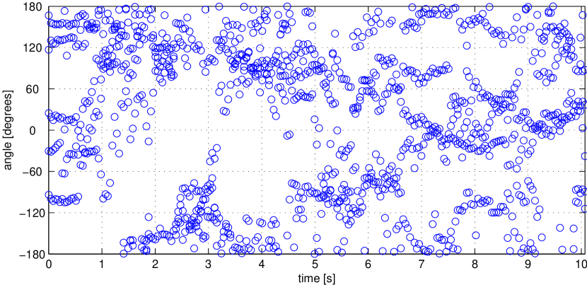
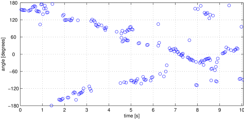
Figure 4: Upper panel illustrates all estimated WGMM means $\mu_{n,k}$ for each time-frame $n$. In the lower panel WGMM means after removing measurements with $\sigma_{n,k}>0.6\;\mathrm{rad}\;(\approx 35^{\circ})$ or $a_{n,k}<0.15$ are illustrated

III-D2 Multi-target DOA tracking implementation

For the actual RBPF implementation we now reintroduce the WGMM component index $k$ and the source index $p$. The state vector is defined individually for each detected source $p=1,\dots,P$ and is denoted hereafter as $\mathbf{s}_{n}^{(p)}$. Similarly the multiple measurements at same time step obtained from the WGMM model are denoted by $\mathbf{m}_{n}^{(k)}=\begin{bmatrix}\cos(\mu_{n,k}),\sin(\mu_{n,k})\end{bmatrix}^{T}$

The RBPF implementation [37] is applied to the measurements $\mathbf{m}_{n}^{(k)}$ with measurement noise $\mathbf{r}_{n}^{(k)}\sim\mathcal{N}(0,\sigma_{n,k}\mathbf{I})$. The multi-target tracker detects the sources and makes the association of $k$th WGMM measurement belonging to one of sources $p=1,\dots,P$. Alternatively, if none of the active source particle distributions indicate a probability higher than the clutter prior probability, then the current measurement is regarded as clutter. The clutter prior probability is a fixed pre-set value to validate the minimum threshold when the observed measurement is linked to existing source.

The output of the tracker is the state of each source $p$ at each time frame, denoted by $\mathbf{s}_{n}^{(p)}$. Extracting the DOA from the tracked source state requires calculating the angle of the vector defined by the 2-D coordinates and thus the resulting DOA trajectories are obtained as

$$\hat{\mu}_{n,p}\leftarrow\operatorname{atan2}2(\mathbf{s}_{n,2}^{(p)}/\mathbf{s}_{n,1}^{(p)}).$$ (14)

The tracking result for a one test signal is illustrated in Figure 5, where the input of the acoustic tracking are the ones depicted in the bottom panel of Figure 4. The test signal is chosen such that it shows two problematic cases, sources start from the same position and intersect at 8 seconds going to the opposite directions. The tracking result indicates that the second source is detected at 2 seconds from the start just when the sources have traveled far enough from each other, resulting to approximately one first word being missed from the second speaker. The tracker is able to maintain the source association and track correctly the trajectories of intersecting sources.

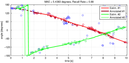
Figure 5: The acoustic tracking result of two sources intersecting and ground truth annotations illustrated when the source is active (voice activity detection by energy thresholding using signal from close-field microphone).

IV Separation model

IV-A Mixture in spatial covariance domain

For the separation part we represent the microphone array signal using mixture SCMs $\mathbf{X}_{fn}\in\mathbb{C}^{M\times M}$. We use magnitude square rooted version of the mixture STFT obtained as,

$$\mathbf{\hat{x}}_{fn}=[|x_{fn1}|^{1/2}\,\mathrm{sign}(x_{fn1}),\dots,|x_{fnM}|^{1/2}\,\mathrm{sign}(x_{fnM})]^{T}$$ (15)

where $\mathrm{sign}(z)=z/|z|$ is the signum function for complex numbers.

The mixture SCM is calculated as $\mathbf{X}_{fn}=\mathbf{\hat{x}}_{fn}\mathbf{\hat{x}}_{fn}^{H}$ for each TF-point ($f,n$). The diagonals of each $\mathbf{X}_{fn}$ contains the magnitude spectrogram of each input channel. The argument and absolute value of $[\mathbf{X}_{fn}]_{m_{1},m_{2}}$ (off-diagonal values) represents the phase difference and magnitude correlation, respectively, between microphones $(m_{1},m_{2})$ for a TF-point ($f,n$).

The TF domain mixing in Equation (2) can be approximated using mixture SCMs as

$$\mathbf{X}_{fn}\approx\mathbf{\hat{X}}_{fn}=\sum_{p=1}^{P}\mathbf{H}_{fn,p}\hat{s}_{fn,p},$$ (16)

where $\hat{s}_{fn,p}=\sqrt{s_{fn,p}s_{fn,p}^{*}}$ is positive real-valued magnitude spectrogram of source $p$ and $\mathbf{H}_{fn,p}=\mathbf{h}_{fn,p}\mathbf{h}_{fn,p}^{H}/||\mathbf{h}_{fn,p}\mathbf{h}_{fn,p}^{H}||_{F}$ are the SCMs of the frequency domain RIRs $\mathbf{h}_{fn,p}$. The mixing Equation (16) is hereafter referred to as spatial covariance domain mixing.

IV-B Multichannel NMF model with time-variant mixing

The proposed algorithm uses multichannel NMF for source spectrogram estimation and it is based on alternating estimation of the source magnitude spectrogram $\hat{s}_{fn,p}$ and its associated spatial properties in the form of the SCMs $\mathbf{H}_{fn,p}$. In all previous works [16, 18, 20] the problem definition has been simplified for stationary sound sources and the SCMs being fixed for all STFT frames $n$ within the analyzed audio segment. Here we present a novel extension of the multichannel NMF model for time-variant mixing.

In multichannel NMF the model for magnitude spectrogram is equivalent to conventional NMF, which is composed of fixed spectral basis and their time-dependent activations. The SCMs can be unconstrained [47] or as proposed in the earlier works of the authors [19, 20] based on a model that represents SCMs as a weighted sum of entities called ”DOA kernels” each containing a phase difference caused by a single direction vector. This ensures SCMs to comply with the array geometry and match with the time-delays the chosen microphone placement allows.

The NMF magnitude model for source magnitude spectrogram is given as

$$\hat{s}_{fn,p}\approx\sum_{q=1}^{Q}b_{q,p}t_{fq}v_{qn},\quad b_{q,p},t_{fq},v_{qn}\geq 0.$$ (17)

Parameters $t_{fq}$ over all frequency indices $f=1,\dots,F$ represent the magnitude spectrum of single NMF component $q$, and $v_{qn}$ denotes the component gain in each frame $n$. One NMF component represents a single spectrally repetitive event estimated from the mixture and one source is modeled as a sum of multiple components. Parameter $b_{q,p}\in[0,1]$ represents a weight associating NMF component $q$ to source $p$. The soft valued $b_{q,p}$ is motivated by different types of sound sources requiring different amount of spectral templates for accurate modeling and learning of the optimal division of components is determined through parameter updates. For example, stationary noise can be represented using only a few NMF components whereas spectrum of speech varies over time and requires many spectral templates to be modeled precisely. Similar strategy for $b_{q,p}$ is used for example in [18]. Typically the final values of $b_{q,p}$ are mostly binary and only few number of NMF components are shared among sources.

The multichannel NMF model with time-variant mixing can be trivially derived from the SCM mixing Equation (16) by substituting the above defined NMF model (17) in it, resulting in

$$\mathbf{X}_{fn}\approx\mathbf{\hat{X}}_{fn}=\sum_{p=1}^{P}\mathbf{H}_{fn,p}\underbrace{\big{[}\sum_{q=1}^{Q}b_{q,p}t_{fq}v_{qn}\big{]}}_{\approx\hat{s}_{fn,p}}.$$ (18)

IV-C Direction of arrival -based SCM model

In order to constrain the spatial behavior of sources over time using information from the acoustic tracking approach or other prior information, the SCMs need to be interpreted by spatial location of each source in each time frame. The SCM model proposed in [19] parametrizes stationary SCMs based on DOA and here we extend the model for time-variant SCMs $\mathbf{H}_{fn,p}$.

Converting the TDOA in Equation (3) to a phase difference results in DOA kernels $\mathbf{W}_{fd}\in\mathbb{C}^{M\times M}$ for a microphone pair $(m_{1},m_{2})$ defined as

$$[\mathbf{W}_{fd}]_{m_{1},m_{2}}=\exp\big{(}j\omega_{f}\tau_{d}({m_{1},m_{2}})\big{)},$$ (19)

where $\tau_{d}({m_{1},m_{2}})$ denotes the time delay caused by a source at a direction $\mathbf{k}_{d}$.

A linear combination of DOA kernal gives the model for time-varying source SCMs defined as

$$\mathbf{H}_{fn,p}=\sum_{d=1}^{D}\mathbf{W}_{fd}z_{nd,p}.$$ (20)

The directions weights $z_{nd,p}$ denote the spatial location and spread of the source $p$ at each time frame $n$.

The direction weights $z_{nd,p}$ can be interpreted as probabilities of source $p$ originating from each direction $d$. In anechoic conditions only one of the directions weights $z_{nd,p}$ in each time frame would be nonzero, i.e., the direct path explains all spatial information of the source, however in reverberant conditions several of the direction weights are active.

The spatial weights corresponding to tracked sources and their DOA trajectories are set using the wrapped Gaussian distribution as

$$z_{nd,p}=\mathcal{N}_{w}(\theta_{d};\hat{\mu}_{n,p},\hat{\sigma}_{n,p}^{2}),$$ (21)

where $\hat{\mu}_{n,p}$ is obtained as specified in Equation (14) and the variance $\hat{\sigma}_{n,p}^{2}$ is used to control the width of the spatial window of source $p$ in the separation model. The goal is to have a large spatial window when the tracker is certain and the output suppressed (small spatial window) when no new measurements from the predicted source position are observed and the tracker state indicates high uncertainty. This strategy is motivated by ensuring that small untracked deviations in source movement do not cause the spatial focus of the separation to veer off momentarily from the target source and lead to suppression of the desired source content. In experimental tests the source spectrogram estimation by multichannel NMF proved to be sensitive to small errors if the spatial window used was very small. The small spatial window in case of no source activity can be motivated from similar perspective, the estimated source spectrogram from very constrained spatial window is less likely to capture spectrogram details of other sources close to the target trajectory.

The acoustic tracker output variance denoted as $\sigma_{n,p}^{2}$ at each time step $n$ indicates the uncertainty of the source being present at its respective predicted direction $\hat{\mu}_{n,p}$. The above specified strategy can be obtained from the tracker output variance by specifying $\hat{\sigma}_{n,p}^{2}=c-\sigma_{n,p}^{2}$ with a constant $c=\max\limits_{n,p}(\sigma_{n,p}^{2})+\min\limits_{n,p}(\sigma_{n,p}^{2})$. The operation maps the maximum output variance to the smallest spatial window and vice versa. In practice value range of $\sigma_{n,p}^{2}$ is restricted to avoid specifying extremely wide and narrow spatial windows and thus the value of constant $c$ is set in advance. The limits for $\sigma_{n,p}^{2}$ are discussed in more details in Section V-C.

The direction weights for each source at each time frame are scaled to unity $l_{1}$-norm ($\sum_{d=1}^{D}z_{nd,p}=1$). This is done to restrict $\mathbf{H}_{fn,p}$ to only model spatial behavior of sources and not affect modeling the overall energy of the sources. Additionally, when the source is considered inactive, i.e., before its birth or after its death, all the direction weights in the corresponding time frame are set to zero. The spatial weights $z_{nd,p}$ corresponding to the tracking result in Figure 5 are illustrated in two top panels of Figure 6. By comparing to Figure 5, it can be seen that when no new measurements are observed the tracker output state variance is high and the spatial weights are concentrated tightly around the mean, whereas in case of high certainty the spatial spread is wider.

In order to model the background noise and diffuse sources, an additional background source is added with direction weights set to one in indices where $\sum_{p}z_{nd,p}<T$ and zero otherwise. The threshold $T$ is set to allow the detected and tracked sources to capture all spatial evidence within approximately +-30 degrees from their estimated DOAs when the certainty for the given source is high. With the chosen background modeling strategy the tracked sources have exclusive prior to model signals originating from the tracked DOA, with the exception of two DOA trajectories intersecting. An example of the background spatial weights is illustrated in bottom panel of Figure 6. Note that the differently colored regions at different times are due to the scaling ($\sum_{d=1}^{D}z_{nd,p}=1$) and different spatial window widths of the tracked sources at the corresponding time indices.

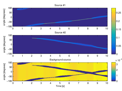
Figure 6: The reconstructed spatial weights as given in Equation (21) for two detected sources are illustrated in two top panels and the spatial weights corresponding to the background source are illustrated in the bottom panel.

IV-D Parameter Estimation

The multichannel NMF model (18) with the time-varying DOA kernel based SCM model (20) and the spatial weights as specified in Equation (21) result to model

$$\mathbf{X}_{fn}\approx\mathbf{\hat{X}}_{fn}=\sum_{p=1}^{P}\underbrace{\sum_{d=1}^{D}\mathbf{W}_{fd}z_{nd,p}}_{\mathbf{H}_{fn,p}}\underbrace{\sum_{q=1}^{Q}b_{q,p}t_{fq}v_{qn}}_{\approx\hat{s}_{fn,p}}.$$ (22)

In order to use the above model for separation, parameters $b_{q,p},t_{fq}$ and $v_{qn}$ defining the magnitude spectrogram modeling part need to be estimated with respect to appropriate optimization criterion.

We use the squared Frobenius norm as the cost function, defined as $\sum_{f=1}^{F}\sum_{n=1}^{N}||\mathbf{X}_{fn}-\mathbf{\hat{X}}_{fn}||^{2}_{F}$. Multiplicative updates for estimating the optimal parameters in an iterative manner can be obtained by partial derivation of the cost function and use of auxiliary variables as in expectation maximization algorithm [48]. The procedure for obtaining multiplicative updates for different multichannel NMF models and optimization criteria are proposed and presented in [18] and can be extended for the new proposed formulation in (22). The entire probabilistic formulation is not repeated here and can be reviewed from [18].

The update equations for the non-negative parameters are

$$b_{q,p} \leftarrow b_{q,p}\frac{\sum_{f,n}t_{fq}v_{qn}\mathrm{tr}(\mathbf{X}_{fn}\mathbf{H}_{fn,p})}{\sum_{f,n}t_{fq}v_{qn}\mathrm{tr}(\mathbf{\hat{X}}_{fn}\mathbf{H}_{fn,p})},$$ (23)

$$t_{fq} \leftarrow t_{fq}\frac{\sum_{n,p}b_{q,p}v_{qn}\mathrm{tr}(\mathbf{X}_{fn}\mathbf{H}_{fn,p})}{\sum_{n,p}b_{q,p}v_{qn}\mathrm{tr}(\mathbf{\hat{X}}_{fn}\mathbf{H}_{fn,p})},$$ (24)

$$v_{qn} \leftarrow v_{qn}\frac{\sum_{f,p}b_{q,p}t_{fq}\mathrm{tr}(\mathbf{X}_{fn}\mathbf{H}_{fn,p})}{\sum_{f,p}b_{q,p}t_{fq}\mathrm{tr}(\mathbf{\hat{X}}_{fn}\mathbf{H}_{fn,p})}.$$ (25)

Note that in contrast to earlier works on multichannel NMF for separation of stationary sound sources [18, 19], we do not update the SCM part $\mathbf{H}_{fn,p}$. It is assumed that the acoustic source tracking and spatial weights of the DOA kernels $\mathbf{W}_{fd}$ fully represent the spatial behavior of the source. This strategy is assessed in more details in discussion Section VI.

IV-E Source separation

For extracting the source signal from the mixture we use combination of single-channel Wiener filter and delay-and-sum beamforming. Separation soft mask ${m}_{fn,p}$ for extracting the source spectrogram from the mixture are obtained using the estimated real valued magnitude spectrogram $\hat{s}_{fn,p}$ to formulate a generalized Wiener filter defined as

$$\mathbf{{y}}_{fn,p}=m_{fn,p}\mathbf{x}_{fn}=\frac{\hat{s}_{fn,p}}{\sum_{p}\hat{s}_{fn,p}}\mathbf{x}_{fn}.$$ (26)

We employ delay-and-sum beamforming to produce single channel source signal from the separated multichannel signals $\mathbf{{y}}_{fn,p}$ (having the mixture signal phase). The final estimate of the sources are given as

$$y_{fn,p}=\mathbf{w}_{fn,p}^{H}\mathbf{{y}}_{fn,p},$$ (27)

where $\mathbf{w}_{fn,p}$ are the DSB weights (steering vector) towards estimated direction of source $p$ at time frame $n$. Finally, the time-domain signal are reconstructed by applying inverse DFT to each frame which are further combined using overlap-add processing.

V Evaluation

In this section we present the objective separation performance and tracking performance of the proposed method using real recordings of moving sound sources. Additionally, we evaluate the separation performance of the proposed algorithm in a setting where the sources are not moving allowing comparison to conventional spatial and spectrogram factorization models assuming stationary sources.

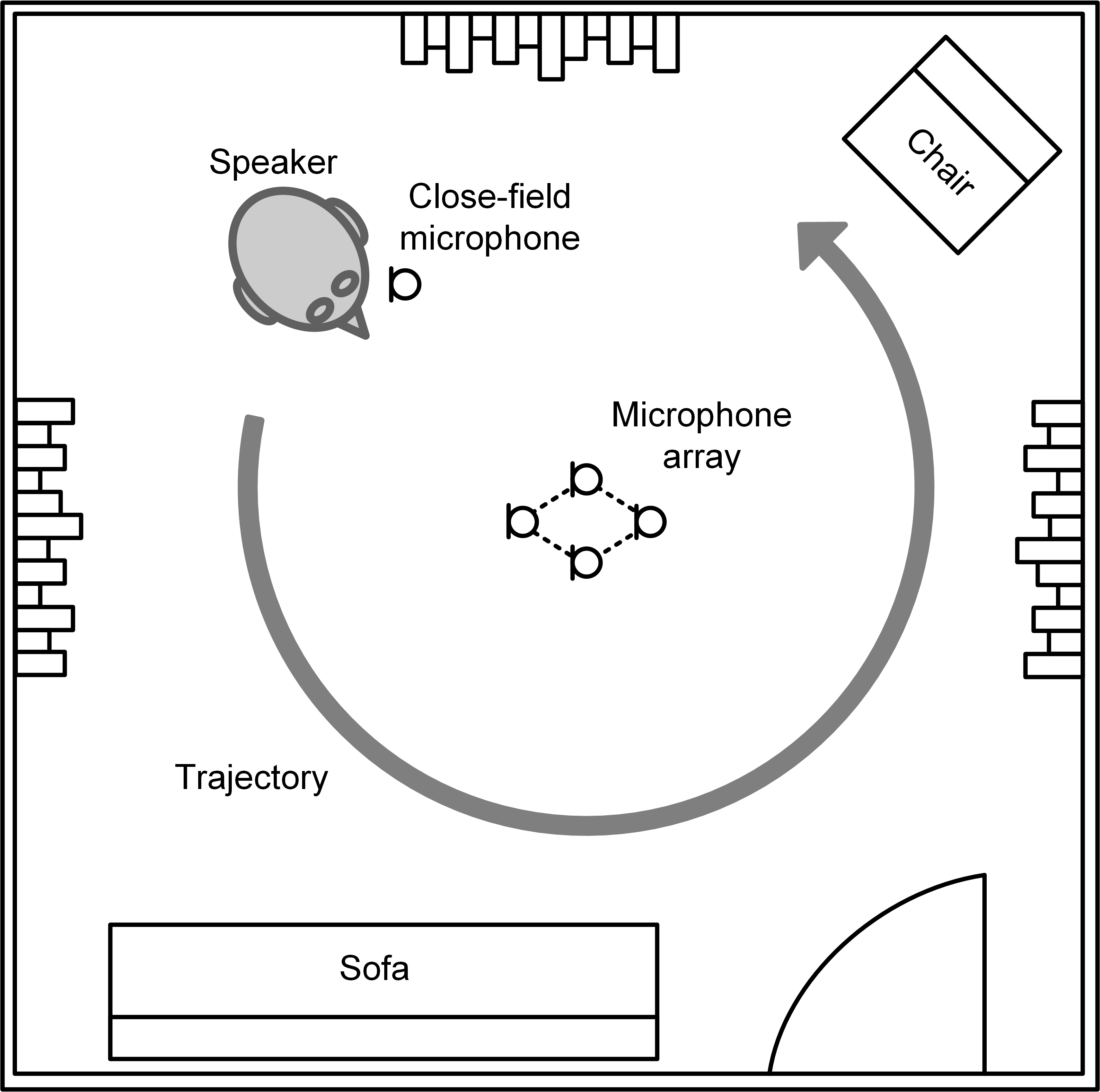
Figure 7: Illustration of the recording setup and the source movement.

V-A Datasets with moving sources

The development and evaluation material was recorded using a compact microphone array consisting of four Sennheiser MKE2 omnidirectional condenser microphones placed on a diamond pattern illustrated in 2 and exact locations of microphones are documented in [19]. The recordings were conducted in an acoustically treated room with dimensions $4.53$ m $\times$ $3.96$ m $\times$ $2.59$ m and reverberation time $T_{60}=$ 0.26 s. The microphone array was placed approximately at the center of the room. Four persons spoke phonetically balanced sentences while walking clockwise (CW) and counterclockwise (CCW) around the microphone array at approximately constant velocity and at average distance of one meter from the array center. The overall assembly of the recordings and the movement of the source is illustrated in Figure 7.

Two CW and two CCW 30-second recordings with four persons were done totaling to 16 signals. All speakers started from the same position and walked on average two times around the array within the recorded 30-second segment. Recordings were done individually allowing producing mixture signals by combining the recordings from different persons. Reference speech signal was captured by a close-field microphone (AKG C520). Additionally, 16 recordings with a loudspeaker playing babble noise and music outside the recording room with the door open were done and considered as a stationary (S) sound source with highly reflected propagation path. The movement of each individual speaker was annotated by hand based on SRP. An example of annotations is illustrated in Figure 5. Note that the annotations are only plotted when the source is active (a simple energy threshold from the close-field microphone signal). The VAD information is only used for evaluation purposes and not by the proposed algorithm.

Three different datasets were generated, one for development and two for evaluation purposes by mixing two and three individual speaker recordings. All mixture utterances in all datasets were 10 seconds in duration. In all datasets the signals were manually cut in such way that speaker trajectories based on the annotations were no closer than $45^{\circ}$ when going in the same direction (CW vs. CW and CCW vs. CCW). Naturally, the trajectories can intersect in the case of opposite directions (CW vs. CCW).

For the development set the first 15 seconds from each recording were used, while the remaining 15 to 30 seconds were used to generate the evaluation sets. In the development set 8 mixtures of two speakers and 16 live recordings were generated and each recording was only used once. The first evaluation dataset consists of 48 mixtures of two speakers using all possible unique combinations of the recordings with different speakers. The second evaluation dataset contains 16 mixtures of three speakers based on a subset of all possible unique combinations. The subset was chosen to represent all different source trajectory combinations (all sources moving in the same direction vs one of the sources moving in the opposite direction). The datasets are summarized in Table I.

The global parameters related to tracking and separation performance of the proposed algorithm were optimized using the development dataset. The recorded signals were downsampled and processed with sampling rate of $F_{s}=24000$ Hz.

TABLE I: Description of datasets.

Developmenet dataset
Number of
samples	Source 1	Source 2	Details
2	CW	CW	$\measuredangle>45^{\circ}$
2	CCW	CCW	$\measuredangle>45^{\circ}$
4	CW	CCW	Sources intersect
12	CW/CCW	S (babble)	SNR = -5, -10 and -15 dB
4	CW/CCW	S (music)	SNR = -10 dB

Evaluation dataset, 2 sources
Number of
samples	Source 1	Source 2	Details
16	CW	CW	$\measuredangle>45^{\circ}$
16	CCW	CCW	$\measuredangle>45^{\circ}$
16	CW	CCW	Sources intersect

Evaluation dataset, 3 sources
Number of
samples	Source 1	Source 2	Source 3	Details
4	CW	CW	CW	$\measuredangle>45^{\circ}$
4	CCW	CCW	CCW	$\measuredangle>45^{\circ}$
4	CW	CW	CCW	Sources intersect
4	CCW	CCW	CW	Sources intersect

Dataset with stationary sources from [19]
Number of
samples	Source 1	Source 2	Details
8 / 8	$45^{\circ}$ / $135^{\circ}$	$90^{\circ}$ / $180^{\circ}$	$\measuredangle=45^{\circ}$
8 / 8	$0^{\circ}$ / $45^{\circ}$	$90^{\circ}$ / $135^{\circ}$	$\measuredangle=90^{\circ}$
8 / 8	$0^{\circ}$ / $45^{\circ}$	$135^{\circ}$ / $180^{\circ}$	$\measuredangle=135^{\circ}$

V-B Dataset with stationary sources

In order to compare the performance of the proposed algorithm against conventional methods assuming stationary sources [18, 19, 20], we include additional evaluation dataset with completely stationary sources. We use the dataset introduced in [19] consisting of two simultaneous sound sources. In short the dataset contains speech, music and noise sources convolved with RIRs from various angles captured in a regular room (7.95 m x 4.90 m x 3.25 m ) with a reverberation time $T_{60}=350$ ms. The array used for recording is exactly the same as the one used in the datasets introduced in Section V-A and more details of the recordings can be found from [19]. In total the dataset contains 48 samples with 8 different source types and 6 different DOA combinations. Each sample is 10 seconds in duration. The different conditions are summarized in last tabular of Table I.

V-C Experimental setup

For the WGMM parameter estimation the peaks in the SRP function were enhanced by exponentiation $S_{dn}^{(3/2)}$, which emphasizes high energy peaks (direct path) and low energy reflected content is decreased. This was found to improve operation in moderate reverberation. A five-component ($K=5$) WGMM model (6) was estimated from the SRP and parameters from a previous frame were used as an initialization for next frame. The criteria for removing WGMM measurements were set to values of $\sigma_{n,k}>0.6\;\mathrm{rad}\;(34^{\circ})$ and $a_{n,k}<0.15$ by visually inspecting the development set results.

The acoustic tracker parameters were optimized by maximizing the development set tracking performance. The parameters were set to the following values. Average variance of the WGMM measurements was scaled to $\sigma^{2}=0.25$ for each processed signal to be in appropriate range for the particle filtering toolbox. The clutter prior probability was fixed for all measurements to $CP=0.1$. In the particle filtering framework the life time of the target is modeled using a gamma distribution with parameters $\alpha$ and $\beta$. The best tracking performance was achieved with $\alpha=3$ and $\beta=4$. The target initial state was fixed to $\mathbf{s}_{n}^{(p)}=[\cos(\pi),\sin(\pi),0.1,0.1]$. The pre-set prior probability of source birth was set to $BP=0.005$.

The parameters of the multichannel NMF algorithm were set as follows: the window length was 2048 samples with 50% overlap and 80 NMF components were used for modeling the magnitude spectrogram. The entire signals were processed as whole. Before restoring the spatial weights by Equation (21) a minimum and maximum variance for $\sigma_{n,p}$ were set to 0.025 and 0.3, respectively. This was done in order to avoid unnecessarily wide or narrow spatial window (as can be seen from Figure 6). With the chosen minimum and maximum values for $\hat{\sigma}_{n,p}^{2}$, the constant in Equation (21) becomes $c=\max(\sigma_{n,p}^{2})+\min(\sigma_{n,p}^{2})=0.325$. The background source threshold for setting the spatial weights active was set to $0.01$, which corresponds to approximately $\pm 30^{\circ}$ exclusive spatial window for the actual tracked sources when the tracker output state variance is at its minimum indicating high certainty of source being present at the predicted direction.

V-D Acoustic tracking performance

The acoustic tracking performance is evaluated against the hand-annotated ground truth source trajectories by using the accuracy (mean absolute error) and recall rate as the metrics. The tracking error for each source in each time frame with $2\pi$ ambiguity is specified as

$$e_{n,p}=\hat{\mu}_{n,p}^{\mathrm{(ann.)}}-\hat{\mu}_{n,p}=\tilde{e}_{n,p}+2\pi N,\quad N\in\mathcal{Z}$$ (28)

where $\hat{\mu}_{n,p}^{\mathrm{(ann.)}}$ denotes the annotated DOA of $p$th source in time frame $n$ and $\hat{\mu}_{n,p}$ is obtained using Equation (14). Using the error term $\tilde{e}$ which is wrapped to $[-\pi,\pi]$, we specify mean-absolute error ($\mathrm{MAE}$) as

$$\mathrm{MAE}=\sum_{p=1}^{\hat{P}}\frac{1}{N}\sum_{n=1}^{N}|\tilde{e}_{n,p}|,$$ (29)

where $\hat{P}$ is the number of annotated sources.

The recall rate is defined as the proportion of time instances the detected source is correctly active with respect to when the source was truly active and emitting sound. The ground truth of the active time instances is obtained by voice activity detection (VAD) using the close-field signal of the source. The VAD is used in order to take into account that some utterances start 1 to 2 seconds after the beginning of the signal even though the annotations are continuous for the whole duration of recordings. Additionally, if the tracked source dies before the end of the signal during a pause of speech, the duration of the pause is not accounted for as a recall error, but the remaining missing part is. We will denote the recall rate using variable $\mathrm{recall}\in[0,1]$.

The proposed method uses multi-target tracker that can detect arbitrary number of sources and trajectories denoted as $P$. For evaluation of tracking and separation performance we need to match the annotated sources $1,...,\hat{P}$ and detected sources $1,...,P$ by searching trough all possible permutations $r$ of the detected sources denoted as $\mathbf{P}_{r}:\{1,...,P\}\rightarrow\{1,...,\hat{P}\}$. The permutation matrix $\mathbf{P}_{r}$ is applied to change the ordering in which detected sources are evaluated against the annotations.

We propose to choose the permutation $r$ for final scoring that maximizes combination of $\mathrm{MAE}$ and $\mathrm{recall}$. First $\mathrm{MAE}$ is converted into a proportional measure $\mathrm{MAER}=1-(\mathrm{MAE}/\pi)\in[0,1]$, where 1 denotes zero absolute error and 0 denotes maximum $\pi\;\mathrm{rad}=180^{\circ}$ tracking error at all times. Summing the $\mathrm{MAER}$ and the recall rate with permutation $r$ applied to the estimated sources equals to

$$\mathrm{F}_{r}=\mathrm{MAER}_{r}+\mathrm{recall}_{r},$$ (30)

which is referred to as overall accuracy. The best permutation for each signal is chosen by finding the minimum value of $\mathrm{F}_{r}$ over all permutations indexed by $r$. The combination of both measures is used to avoid favoring permutations with very short detected trajectories with small $\mathrm{MAE}$ over longer trajectories with slightly larger $\mathrm{MAE}$, for example accurate tracking of a single word from the entire utterance. Additionally, we do not consider and compensate for cases where one sound source is correctly tracked by two trajectories with discontinuity during the pauses in speech. The effect of this is negligible due to the short test signals used (10 seconds).

The acoustic tracking performance averaged over all signals in all datasets and source detection performance is reported in Table II. The tracking error measured by $\mathrm{MAE}$ is below 10 degrees for datasets with two sources, which can be regarded as a good result. Noticeably the accuracy of the tracking is even better with the evaluation dataset. However the recall rate drops by 4% mostly due to late detection of sources, which displays the difficulty of setting the optimal values for parameters controlling the birth and death of sources in the particle filtering. In general, a low recall rate can be considered as conservative and only detecting and tracking dominant portions of sources. Alternatively, optimizing the parameters for 100% recall rate would lead to detection of numerous phantom sources, caused by reverberation and noise in the recordings. The recall rate and tracking accuracy are noticeably decreased for the evaluation dataset with three simultaneous sources.

As indicated by the second chart in Table II, the percentage of correctly detected number of sources is approximately 80% for both two source datasets and drops down to 56% for the dataset with three sources. The errors in source detection are mostly caused by overdetection in the case of two simultaneous sources, whereas in the more difficult scenario of three sources the underdetection is also a significant cause of error.

TABLE II: Acoustic tracking results.

Tracking performance
	Dev.	Eval.	Eval.
Criteria	(2 sources)	(2 sources)	(3 sources)
$\mathrm{MAE}$	$~{}7.3^{\circ}$	$~{}6.1^{\circ}$	$10.5^{\circ}$
$\mathrm{recall}$	86.3%	82.2%	64.7%

Source detection performance
	Dev.	Eval.	Eval.
Criteria	(2 sources)	(2 sources)	(3 sources)
$P==\hat{P}$	79.2%	81.3%	50.0%
$P>\hat{P}$	20.8%	16.7%	25.0%
$P<\hat{P}$	0.0%	2.0%	25.0%

V-E Source separation performance

V-E1 Separation evaluation criteria

We evaluate the separation performance of the proposed algorithm using the following objective separation criteria with the close-field microphone signal as a reference. From the separation evaluation toolbox proposed in [38] we have included signal-to-distortion ratio (SDR) and signal-to-interference ratio (SIR) evaluated in short segments of 200 ms. The score of each segment in dB scale is converted to linear scale and averaged over all segments after which the resulting average is converted back to dB scale. The resulting metrics are abbreviated as segmental SDR (SSDR) and segmental SIR (SSIR). The use of segmental evaluation was chosen due to the operation of BSSeval, which projects the separated signal into reference signal subspace and assumes that this projection is stationary. However, in the case of moving sound sources and reference by close-field microphone the initial delay to the far-field array and the room reflections change from frame to frame which requires the projection operator to be also time-variant. This is achieved by assuming projection stationarity within each 200ms segment. Other metrics include the short-time objective intelligibility measure (STOI) [39] which is used to predict the intelligibility of the separated speech in comparison to the reference signal, and the frequency-weighted segmental signal-to-noise ratio (fwSegSNR) [40]. The latter metrics, STOI and fwSeqSNR, were calculated without segmenting.

V-E2 Reference methods

The description of methods whose separation performance is evaluated are given in Table III and can be summarized as follows. The plain microphone signal from the array acts as a lowest performance baseline whereas the IRM indicates an upper limit. The tracking information is also used in the beamforming (DSB and MVDR) to specify the weights $\mathbf{w}_{fn,p}^{H}$ to enhance the signal at each time frame originating from the estimated DOA. The separation performance of proposed method was also evaluated using the ground truth DOA trajectories for specifying the source movement for the multichannel NMF part. This evaluation indicates the highest achievable separation performance with perfect tracking information and the results can be also used for validating the robustness of the overall proposed separation algorithm towards small tracking errors.

The MVDR beamforming was implemented using the sample covariance method [42] for estimating the noise covariance matrix. The noise covariance was estimated from $M=20$ previous frames with respect to each processed frame and it captures the stationary noise statistics as well as the immediate spectral details of interfering speech sources. Additionally, a diagonal loading ($\sigma=5$) of noise covariance matrices was applied to improve robustness of the MVDR beamformer. These parameters were optimized using the development set.

TABLE III: Description of compared separation methods.

Abbrv.	Description
mic	Microphone signal from the array (ch #1).
DSB	Delay-and-sum beamforming.
MVDR	Minimum variance distortionless beamforming.
MNMF sta.	Multichannel NMF assuming stationary sources [20].
MNMF	Proposed method, i.e. multichannel NMF with time-varying SCM model.
MNMF ann.	Proposed method with ground truth annotations as source trajectories.
IRM	Ideal ratio mask separation.

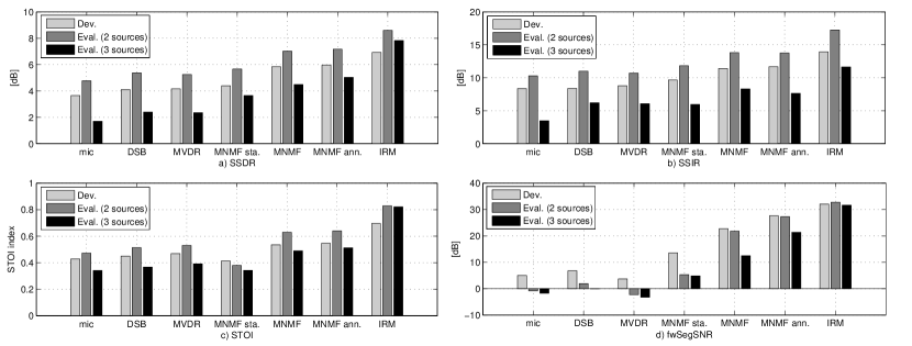
Figure 8: Separation performance measured using various objective separation criteria: SSDR, SSIR, STOI, fwSegSNR.

V-E3 Separation results

The separation performance measured by SSDR, SSIR, STOI and fwSegSNR is calculated with the source permutation obtained by minimizing the accuracy criterion specified in Equation (30) and the results are averaged over all sources and mixtures. The separation performance for all the tested methods with all the considered criteria are given in Figure 8 (a)-(d).

Evaluation with the mixture signal (mic) indicates a baseline performance resulting to SSDR of approximately 4 dB for two simultaneous sources and 2 dB for three sources. Such high absolute performance for mixture signal is because of the segmental evaluation. In contrast, evaluating the entire signals in one segment resulted into negative average SDR for all tested methods (from -6 dB SDR for the mixture to -1 dB for the IRM) while the relative differences remained the same as reported in the Figure 8. The absolute results obtained this way did not reflect the subjective separation performance and are not reported in the paper. The overall low scores were assumed to be caused by the problems of projection operation in BSSeval toolkit, discussed in the beginning of Section V-E.

The beamforming methods, DSB and MVDR, consistently improve SSDR, SSIR and STOI in comparison to microphone signal. However, the overall improvement in all datasets is relatively poor: SSDR improvement varies from 0.45 dB to 0.70 dB, and STOI barely reaches the index of 0.5, indicating low predicted intelligibility for the separated sources. Additionally, MVDR beamforming has negative effect on the fwSegSNR criterion, which may be caused by unwanted canceling of target source due to the rudimentary noise covariance estimation method employed. DSB on the other hand does not have this negative effect. With all other evaluated criteria MVDR beamforming exceeds the DSB performance with a small margin.

When violating the moving sources assumption and using multichannel NMF aimed for separation of stationary sound sources [20], the performance is poor especially with STOI that decreases below the array microphone baseline. The other evaluated metrics are similar to beamforming approaches. When the source is momentarily at the target static direction (blindly estimated in [20]) the separation quality is high, but as the source moves it shifts out of spatial focus of the separation.

The results regarding the proposed method can be summarized by stating that it significantly increases the separation performance over the beamforming methods DSB and MVDR: in case of two sources the SSDR improves approximately by 1.5 dB and improvement is even greater for three simultaneous sources (2 dB). SSIR improvement follows the trend of SSDR and STOI increases approximately by an index of 0.1. The use of ground truth annotations in the case of two simultaneous sources does not significantly increase the performance: SSDR increases only by 0.13 dB and 0.15 dB, SSIR is unchanged and STOI increases by 0.01. This validates the good acoustic tracking results reported in Table II. The separation performance with the three sources follows the poorer tracking performance and the use of annotations has greater impact on improving the objective criteria, SSDR is increased by 0.5 dB by use of annotations but interestingly the SSIR decreases. This may be due to the annotations being always active even if the speech starts 1 to 2 seconds from the beginning of the signal resulting to nonzero separation output for the annotations, whereas in the actual tracking implementation the source signal is truly zero until it is detected.

The behavior of all methods with all criteria is consistent with all datasets. Although the absolute differences in objective intelligibility are small, the increase in STOI by the proposed method over the beamforming methods is greater than the STOI improvement by beamforming over the microphone signal. The overall difficulty of each dataset can be estimated from the IRM performance, which indicates that the actual evaluation dataset with two sources is less difficult than the development dataset. The performance gap between the proposed method and IRM separation is considerable especially in case of three simultaneous sources. This is due to the fact that IRM is not much affected by the adding of third source, since speech is relatively sparse in time frequency domain and good separation can be achieved with oracle masks even with three simultaneous speakers. Evaluation of IRM performance by SSDR and SSIR for two source dataset indicates not as big difference in comparison to the proposed method. However, the IRM performance is also limited by the fact that far-field and close-field signal spaces are extremely different and time-frequency masking cannot recover the close-field signal perfectly due to mixture phase is used. In subjective evaluation IRM preserves the intelligibility of the speech much better than any separation method which is also indicated by the good results in the objective evaluation of intelligibility, i.e. STOI for IRM is around 0.7-0.8.

As a final result we provide a comparison of separation performance obtained with similar DOA-based spatial and spectrogram factorization models assuming stationary sources [18, 19, 20]. The evaluation dataset consist of all sources being stationary, see Section V-B. The proposed algorithm was run as is with the exception that source reconstruction was done without DSB, since the reference signals are reverberated source signals and evaluation in [20] is based on the spatial images of the sources [49]. The details of evaluation procedure and reference results are as presented in [20]. In theory, if the source DOA trajectory estimation would be perfect, similar results between multichannnel NMF-based methods regardless of source movement assumption should be obtained. However, methods proposed in [19, 20] also update elements of the DOA kernels (Equation (19)) whereas in this work they are fixed to analytic anechoic array responses.

The SDR, SIR, SAR and ISR are given in Table IV, which shows that the SDR performance of the proposed method is lower in comparison to methods utilizing the stationary assumption, while SIR is highest among the tested methods. The average tracking error (MAE) for the dataset was $8.8^{\circ}$ and recall rate was 79% which are similar to the tracking performance for other 2 source datasets given in Table II. The comparison to multichannel NMF models assuming stationary source motivates the future work for reducing the performance gap while assuming moving sound sources and possible research directions are discussed in the next section.

Method	SDR	SIR	SAR	ISR
MNMF proposed	3.2 dB	9.0 dB	7.0 dB	5.8 dB
MNMF sta. [20]	5.6 dB	6.8 dB	13.1 dB	9.9 dB
MNMF sta. [19]	4.8 dB	8.1 dB	10.3 dB	10.5 dB
MNMF sta. [47]	3.7 dB	4.5 dB	12.7 dB	8.4 dB
ICA [50]	2.0 dB	4.5 dB	8.2 dB	6.9 dB

TABLE IV: Results of dataset and methods from [19] and [47] with two simultaneous stationary sources.

VI Discussion

In this section we present a few remarks regarding the algorithm development choices and possible future work for improving and extending the method.

The strategy of using the estimated source DOA trajectories for definition of the SCM model in (22) means effectively using only channel-wise time differences and assuming anechoic environment. This strategy can be questioned in comparison to also updating the channel-wise level differences as in [19, 20]. However, the difficulty of updating the level differences between input channels lies within the fact that with moving sources there may be only very few frames of data observed from each direction and investigation of the updating $\mathbf{W}_{fd}$ in such setting was left for future work.

The multichannel NMF model (22) would allow to use multichannel Wiener filter (MWF) for source reconstruction as in [18]. Informal experiments showed inferior performance with MWF in comparison to chosen combination of single-channel Wiener filter and DSB. There are several possible reasons to explain the findings. The multichannel model used for representing source SCMs relies only on the anechoic responses which can be suboptimal for constructing the MVF for source reconstruction. Additionally, errors in source SCM estimation can lead to unexpectedly sharp spectral and spatial responses for source reconstruction with MVF. The strategy of single-channel Wiener filter and DSB is argued to be less destructive with respect small estimation errors.

Analysis of the tracking performance indicated that fairly accurate source DOA trajectories can be estimated with existing methods in realistic capturing conditions which justifies the applicability of the proposed separation algorithm for general use. Tracking errors may be caused by erroneously representing a single source with two consecutive but separate tracks due to pauses in speech. Also in the case of intersecting DOA trajectories, the estimated tracks can switch the actual acoustic targets, i.e., source 1 continues to track acoustic evidence of source 2 and vice versa. It should be noted that we did not account for the above problems in the tracking and separation performance evaluation.

The extremely good results of using of deep learning for speech separation [10, 11, 51] are quickly replacing the use factorization based models in source separation. With multichannel audio the spatial parameters being complex-valued require use of other approaches for SCM estimation, for example in [52] DNNs are used for spectrogram estimation while SCMs are estimated using a probabilistic model and EM-algorithm. The strength of the proposed method compared to DNN-based separation is that it operates on spatial information and spectral factorization of the observed data only and works relatively well in any scenario and all sound content (music, noise, everyday sounds) without any training material.

VII Conclusions

In this article a separation method for moving sound sources based on acoustic tracking and separation mask estimation by multichannel non-negative matrix factorization was proposed. We analyzed the objective separation performance and the proposed method exceeded the conventional beamforming using the same tracking information by a fair margin. The comparison against ground truth source DOA trajectories indicated only minor impairment to objective separation performance. Additionally, analysis of the acoustic tracking realization showed good performance, recall rate over 80 % and absolute tracking error less than 10 degrees with two simultaneous moving sound sources. In conclusion the proposed method was shown to be robust and capable of separating at least two moving targets from mixtures recorded with a compact sized microphone array in realistic capturing conditions.

References

- [1] J. Barker, R. Marxer, E. Vincent, and S. Watanabe, “The third CHiME speech separation and recognition challenge: Dataset, task and baselines,” in 2015 IEEE Workshop on Automatic Speech Recognition and Understanding (ASRU). IEEE, 2015, pp. 504–511.
- [2] Y. Liu, P. Zhang, and T. Hain, “Using neural network front-ends on far field multiple microphones based speech recognition,” in Proceedings of IEEE International Conference on Acoustics, Speech and Signal Processing (ICASSP). IEEE, 2014, pp. 5542–5546.
- [3] V. Valimaki, A. Franck, J. Ramo, H. Gamper, and L. Savioja, “Assisted listening using a headset: Enhancing audio perception in real, augmented, and virtual environments,” IEEE Signal Processing Magazine, vol. 32, no. 2, pp. 92–99, 2015.
- [4] T. Heittola, A. Mesaros, T. Virtanen, and M. Gabbouj, “Supervised model training for overlapping sound events based on unsupervised source separation.” in Proceedings of IEEE International Conference on Acoustics, Speech and Signal Processing, 2013, pp. 8677–8681.
- [5] P. Smaragdis, “Blind separation of convolved mixtures in the frequency domain,” Neurocomputing, vol. 22, no. 1, pp. 21–34, 1998.
- [6] F. Nesta, P. Svaizer, and M. Omologo, “Convolutive BSS of short mixtures by ICA recursively regularized across frequencies,” IEEE Transactions on Audio, Speech, and Language Processing, vol. 19, no. 3, pp. 624–639, 2011.
- [7] A. Jourjine, S. Rickard, and O. Yilmaz, “Blind separation of disjoint orthogonal signals: Demixing n sources from 2 mixtures,” in Proceedings of IEEE International Conference on Acoustics, Speech, and Signal Processing (ICASSP), vol. 5. IEEE, 2000, pp. 2985–2988.
- [8] O. Yilmaz and S. Rickard, “Blind separation of speech mixtures via time-frequency masking,” IEEE transactions on Signal Processing, vol. 52, no. 7, pp. 1830–1847, 2004.
- [9] S. Rickard and O. Yilmaz, “On the approximate W-disjoint orthogonality of speech,” in Proceedings of IEEE International Conference on Acoustics, Speech, and Signal Processing (ICASSP), 2002, pp. 529–532.
- [10] A. Narayanan and D. Wang, “Ideal ratio mask estimation using deep neural networks for robust speech recognition,” in Proceedings of IEEE International Conference on Acoustics, Speech and Signal Processing (ICASSP), Vancouver, Canada, 2013, pp. 7092–7096.
- [11] F. Weninger, J. R. Hershey, J. Le Roux, and B. Schuller, “Discriminatively trained recurrent neural networks for single-channel speech separation,” in Proceedings of IEEE Global Conference on Signal and Information Processing (GlobalSIP). IEEE, 2014, pp. 577–581.
- [12] A. A. Nugraha, A. Liutkus, and E. Vincent, “Multichannel music separation with deep neural networks,” in European Signal Processing Conference (EUSIPCO), 2016.
- [13] ——, “Multichannel audio source separation with deep neural networks,” in Research Report RR-8740, Inria., 2015.
- [14] J. T. Geiger, J. F. Gemmeke, B. Schuller, and G. Rigoll, “Investigating NMF speech enhancement for neural network based acoustic models,” Proceedings of the Annual Conference of International Speech Communication Association (INTERSPEECH), 2014.
- [15] J. F. Gemmeke, T. Virtanen, and A. Hurmalainen, “Exemplar-based sparse representations for noise robust automatic speech recognition,” IEEE Transactions on Audio, Speech, and Language Processing, vol. 19, no. 7, pp. 2067–2080, 2011.
- [16] A. Ozerov and C. Fevotte, “Multichannel nonnegative matrix factorization in convolutive mixtures for audio source separation,” IEEE Transactions on Audio, Speech, and Language Processing, vol. 18, no. 3, pp. 550–563, 2010.
- [17] S. Arberet, A. Ozerov, N. Q. Duong, E. Vincent, R. Gribonval, F. Bimbot, and P. Vandergheynst, “Nonnegative matrix factorization and spatial covariance model for under-determined reverberant audio source separation,” in Proceedings of International Conference on Information Sciences Signal Processing and their Applications (ISSPA), 2010.
- [18] H. Sawada, H. Kameoka, S. Araki, and N. Ueda, “Multichannel extensions of non-negative matrix factorization with complex-valued data,” IEEE Transactions on Audio, Speech, and Language Processing, vol. 21, no. 5, pp. 971–982, 2013.
- [19] J. Nikunen and T. Virtanen, “Direction of arrival based spatial covariance model for blind sound source separation,” IEEE Transactions on Audio, Speech, and Language Processing, vol. 22, no. 3, pp. 727–739, 2014.
- [20] ——, “Multichannel audio separation by direction of arrival based spatial covariance model and non-negative matrix factorization,” in Proceedings of IEEE International Conference on Acoustic, Speech and Signal Processing. IEEE, 2014, pp. 6727–6731.
- [21] R. Mukai, H. Sawada, S. Araki, and S. Makino, “Robust real-time blind source separation for moving speakers in a room,” in Proceedings of International Conference on Acoustics, Speech, and Signal Processing (ICASSP), vol. 5. IEEE, 2003, pp. V–469.
- [22] ——, “Blind source separation for moving speech signals using blockwise ICA and residual crosstalk subtraction,” IEICE Transactions on Fundamentals of Electronics, Communications and Computer Sciences, vol. 87, no. 8, pp. 1941–1948, 2004.
- [23] J. Málek, Z. Koldovskỳ, and P. Tichavskỳ, “Semi-blind source separation based on ICA and overlapped speech detection,” in Latent Variable Analysis and Signal Separation. Springer, 2012, pp. 462–469.
- [24] D. Kounades-Bastian, L. Girin, X. Alameda-Pineda, S. Gannot, and R. Horaud, “A variational em algorithm for the separation of time-varying convolutive audio mixtures,” IEEE/ACM Transactions on Audio, Speech, and Language Processing, vol. 24, no. 8, pp. 1408–1423, 2016.
- [25] T. Higuchi, N. Takamune, T. Nakamura, and H. Kameoka, “Underdetermined blind separation and tracking of moving sources based on DOA-HMM,” in Acoustics, Speech and Signal Processing (ICASSP), 2014 IEEE International Conference on. IEEE, 2014, pp. 3191–3195.
- [26] M. S. Brandstein and H. F. Silverman, “A practical methodology for speech source localization with microphone arrays,” Computer Speech & Language, vol. 11, no. 2, pp. 91–126, 1997.
- [27] U. Klee, T. Gehrig, and J. McDonough, “Kalman filters for time delay of arrival-based source localization,” EURASIP Journal on Applied Signal Processing, vol. 2006, pp. 167–167, 2006.
- [28] S. Gannot and T. G. Dvorkind, “Microphone array speaker localizers using spatial-temporal information,” EURASIP journal on applied signal processing, vol. 2006, pp. 174–174, 2006.
- [29] J. Vermaak and A. Blake, “Nonlinear filtering for speaker tracking in noisy and reverberant environments,” in Proceedings of Internation conference on Acoustics, Speech, and Signal Processing (ICASSP), vol. 5. IEEE, 2001, pp. 3021–3024.
- [30] D. B. Ward, E. A. Lehmann, and R. C. Williamson, “Particle filtering algorithms for tracking an acoustic source in a reverberant environment,” IEEE Transactions on Speech and Audio Processing, vol. 11, no. 6, pp. 826–836, 2003.
- [31] S. Särkkä, A. Vehtari, and J. Lampinen, “Rao-Blackwellized particle filter for multiple target tracking,” Information Fusion, vol. 8, no. 1, pp. 2–15, 2007.
- [32] ——, “Rao-Blackwellized Monte Carlo data association for multiple target tracking,” in Proceedings of the seventh international conference on information fusion, vol. 1. I, 2004, pp. 583–590.
- [33] X. Zhong and J. R. Hopgood, “Time-frequency masking based multiple acoustic sources tracking applying Rao-Blackwellised Monte Carlo data association,” in IEEE Workshop on Statistical Signal Processing. IEEE, 2009, pp. 253–256.
- [34] J. Traa and P. Smaragdis, “A wrapped Kalman filter for azimuthal speaker tracking,” IEEE Signal Processing Letters, vol. 20, no. 12, pp. 1257–1260, 2013.
- [35] ——, “Multichannel source separation and tracking with RANSAC and directional statistics,” IEEE/ACM Transactions on Audio, Speech, and Language Processing, vol. 22, no. 12, pp. 2233–2243, 2014.
- [36] Y. Agiomyrgiannakis and Y. Stylianou, “Wrapped Gaussian mixture models for modeling and high-rate quantization of phase data of speech,” IEEE Transactions on Audio, Speech, and Language Processing, vol. 17, no. 4, pp. 775–786, 2009.
- [37] J. Hartikainen and S. Särkkä, “RBMCDAbox-Matlab toolbox of Rao-Blackwellized data association particle filters,” documentation of RBMCDA Toolbox for Matlab V, 2008.
- [38] E. Vincent, R. Gribonval, and C. Févotte, “Performance measurement in blind audio source separation,” IEEE Transactions on Audio, Speech, and Language Processing, vol. 14, no. 4, pp. 1462–1469, 2006.
- [39] C. H. Taal, R. C. Hendriks, R. Heusdens, and J. Jensen, “An algorithm for intelligibility prediction of time–frequency weighted noisy speech,” IEEE Transactions on Audio, Speech, and Language Processing, vol. 19, no. 7, pp. 2125–2136, 2011.
- [40] Y. Hu and P. C. Loizou, “Evaluation of objective quality measures for speech enhancement,” IEEE Transactions on Audio, Speech, and Language Processing, vol. 16, no. 1, pp. 229–238, 2008.
- [41] S. Srinivasan, N. Roman, and D. Wang, “Binary and ratio time-frequency masks for robust speech recognition,” Speech Communication, vol. 48, no. 11, pp. 1486–1501, 2006.
- [42] I. Tashev, Sound Capture and Processing: Practical Approaches. John Wiley & Sons Inc, 2009.
- [43] P. Smaragdis and P. Boufounos, “Learning source trajectories using wrapped-phase hidden markov models,” in Proceedings of the IEEE Workshop on Applications of Signal Processing to Audio and Acoustics (WASPAA). IEEE, 2005, pp. 114–117.
- [44] J. Traa, “Multichannel source separation and tracking with phase differences by random sample consensus,” Master’s thesis, Graduate College of the University of Illinois at Urbana-Champaign, 2013.
- [45] C. Spille, B. Meyer, M. Dietz, and V. Hohmann, “Binaural scene analysis with multidimensional statistical filters,” in The technology of binaural listening. Springer, 2013, pp. 145–170.
- [46] H. Nies, O. Loffeld, and R. Wang, “Phase unwrapping using 2D-Kalman filter-potential and limitations,” in International Geoscience and Remote Sensing Symposium, vol. 4. IEEE, 2008, pp. 1213–1216.
- [47] H. Sawada, H. Kameoka, S. Araki, and N. Ueda, “New formulations and efficient algorithms for multichannel NMF,” in IEEE Workshop on Applications of Signal Processing to Audio and Acoustics (WASPAA). IEEE, 2011, pp. 153–156.
- [48] A. P. Dempster, N. M. Laird, and D. B. Rubin, “Maximum likelihood from incomplete data via the EM algorithm,” Journal of the Royal Statistical Society, vol. 39, no. 1, pp. 1–38, 1977.
- [49] E. Vincent, H. Sawada, P. Bofill, S. Makino, and J. P. Rosca, “First stereo audio source separation evaluation campaign: data, algorithms and results,” in International Conference on Independent Component Analysis and Signal Separation. Springer, 2007, pp. 552–559.
- [50] H. Sawada, S. Araki, R. Mukai, and S. Makino, “Grouping separated frequency components by estimating propagation model parameters in frequency-domain blind source separation,” IEEE Transactions on Audio, Speech, and Language Processing, vol. 15, no. 5, pp. 1592–1604.
- [51] Y. Isik, J. L. Roux, Z. Chen, S. Watanabe, and J. R. Hershey, “Single-channel multi-speaker separation using deep clustering,” arXiv preprint arXiv:1607.02173, 2016.
- [52] A. A. Nugraha, A. Liutkus, and E. Vincent, “Multichannel audio source separation with deep neural networks,” in IEEE/ACM Transactions on Audio, Speech, and Language Processing, vol. 24, no. 10, 2016, pp. 1652–1664.