OGLE-2016-BLG-1190Lb: First Spitzer Bulge Planet Lies Near the Planet/Brown-Dwarf Boundary

Abstract

We report the discovery of OGLE-2016-BLG-1190Lb, which is likely to be the first Spitzer microlensing planet in the Galactic bulge/bar, an assignation that can be confirmed by two epochs of high-resolution imaging of the combined source-lens baseline object. The planet’s mass $M_{p}=13.4\pm 0.9\,M_{J}$ places it right at the deuterium burning limit, i.e., the conventional boundary between “planets” and “brown dwarfs”. Its existence raises the question of whether such objects are really “planets” (formed within the disks of their hosts) or “failed stars” (low mass objects formed by gas fragmentation). This question may ultimately be addressed by comparing disk and bulge/bar planets, which is a goal of the Spitzer microlens program. The host is a G dwarf $M_{\rm host}=0.89\pm 0.07\,M_{\odot}$ and the planet has a semi-major axis $a\sim 2.0\,{\rm AU}$. We use Kepler K2 Campaign 9 microlensing data to break the lens-mass degeneracy that generically impacts parallax solutions from Earth-Spitzer observations alone, which is the first successful application of this approach. The microlensing data, derived primarily from near-continuous, ultra-dense survey observations from OGLE, MOA, and three KMTNet telescopes, contain more orbital information than for any previous microlensing planet, but not quite enough to accurately specify the full orbit. However, these data do permit the first rigorous test of microlensing orbital-motion measurements, which are typically derived from data taken over $<1\%$ of an orbital period.

1 Introduction

The discovery of Spitzer microlensing planet OGLE-2016-BLG-1190Lb is remarkable in five different respects. First, it is the first planet in the Spitzer Galactic-distribution sample that likely lies in the Galactic bulge, which would break the trend from the three previous members of this sample. Second, it is precisely measured to be right at the edge of the brown dwarf desert. Since the existence of the brown dwarf desert is the signature of different formation mechanisms for stars and planets, the extremely close proximity of OGLE-2016-BLG-1190Lb to this desert raises the question of whether it is truly a “planet” (by formation mechanism) and therefore reacts back upon its role tracing the Galactic distribution of planets, just mentioned above. Third, it is the first planet to enter the Spitzer “blind” sample whose existence was recognized prior to its choice as a Spitzer target. This seeming contradiction was clearly anticipated by Yee et al. (2015b) when they established their protocols for the Galactic distribution experiment. The discovery therefore tests the well-defined, but intricate procedures devised by Yee et al. (2015b) to deal with this possibility. Fourth, it is the first planet (and indeed the first microlensing event) for which the well-known microlens-parallax degeneracy has been broken by observations from two satellites. Finally, it is the first microlensing planet for which a complete orbital solution has been attempted. While this attempt is not completely successful in that a one-dimensional degeneracy remains, it is an important benchmark on the road to such solutions.

In view of the diverse origins and implications of this discovery, we therefore depart from the traditional form of introductions and begin by framing this discovery with four semi-autonomous introductory subsections.

1.1 Microlens Parallax from One and Two Satellites

When Refsdal (1966) first proposed to measure microlens parallaxes using a satellite in solar orbit, a quarter century before the first microlensing event, he already realized that this measurement would be subject to a four-fold degeneracy, and further, that this degeneracy could be broken by observations from a second satellite. See also Gould (1994b) and Calchi Novati & Scarpetta (2016). The microlens parallax is a vector

$${\mbox{\boldmath$\pi$}}_{\rm E}\equiv\pi_{\rm E}{{\mbox{\boldmath$\mu$}}_{\rm rel}\over\mu_{\rm rel}};\qquad\pi_{\rm E}\equiv{\pi_{\rm rel}\over\theta_{\rm E}},$$ (1)

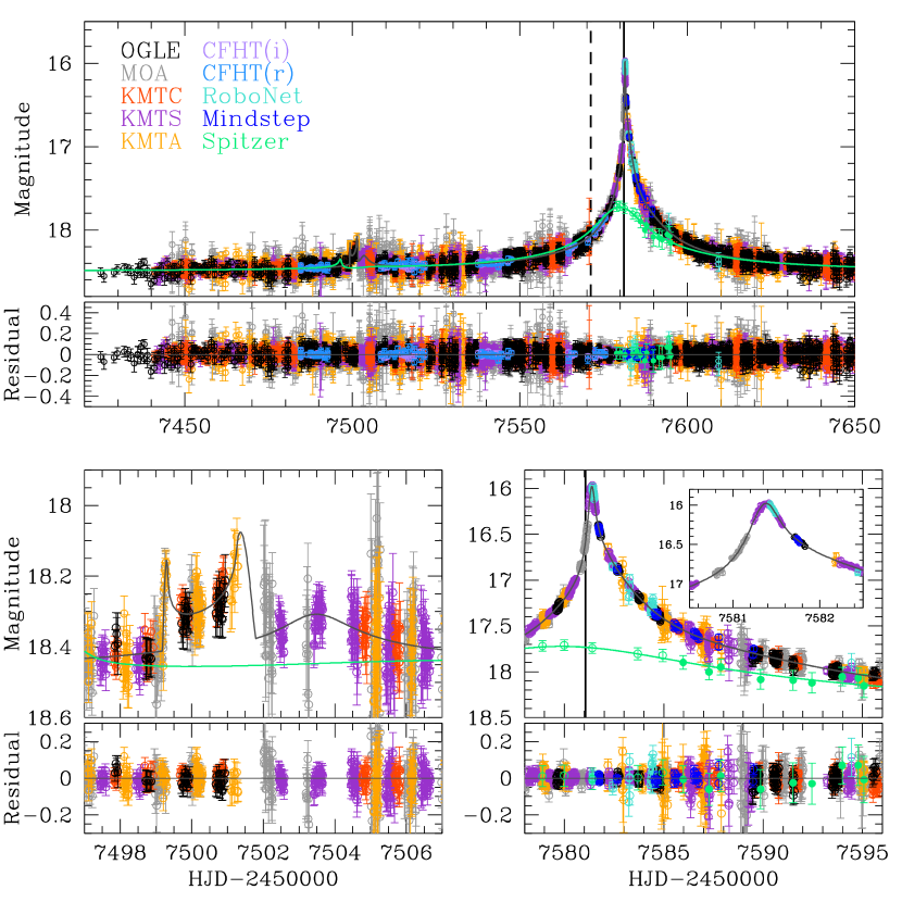
Figure 1: Light curve of OGLE-2016-BLG-1190. The data points are colored as indicated by observatory in the top panel, which shows the full light curve. Fluxes $f_{i}$ from observatory $i$ (including Spitzer) are aligned to the OGLE scale by $f^{\prime}_{i,\rm obs}=(f_{i,\rm obs}-f_{b,i})(f_{s,\rm ogle}/f_{s,i})+f_{b,\rm ogle}$. Models are shown for ground-based and Spitzer data in black and green, respectively. Vertical dashed and solid lines indicate the subjective and objective selection dates for Spitzer observations, respectively. Open and filled circles for Spitzer data (green) show observations initiated by the subjective and objective selection, respectively. Lower panels show zooms of the planetary-caustic crossing (left) and central-caustic cusp approach (right).

whose amplitude is the ratio of the lens-source relative parallax $\pi_{\rm rel}={\rm AU}(D_{L}^{-1}-D_{S}^{-1})$ to the Einstein radius $\theta_{\rm E}$, and whose direction is that of the lens-source relative proper motion ${\mbox{\boldmath$\mu$}}_{\rm rel}$. As illustrated by Figure 1 of Gould (1994b) (compare to Figure 1 of Yee et al. 2015a) observers from Earth and a satellite will see substantially different light curves. By comparing the two light curves, one can infer the vector offset within the Einstein ring of the source as seen from the two observers. Combining this vector offset with the known projected offset of the satellite and Earth, one can then infer ${\mbox{\boldmath$\pi$}}_{\rm E}$.

However, this determination is in general subject to a four-fold degeneracy. While the component of the vector offset in the direction of lens-source motion ${\mbox{\boldmath$\mu$}}_{\rm rel}$ gives rise to an offset in peak times of the event and can therefore be determined unambiguously, the component transverse to this motion must be derived from a comparison of the impact parameters, which leads to a four-fold ambiguity. That is, the impact parameter is a signed quantity but only its magnitude can be readily determined from the light curve.

By far, the most important aspect of this degeneracy is that the source may be either on the same or opposite sides of lens as seen from the two observatories. The parallax amplitude $\pi_{\rm E}$ will be smaller in the first case than the second, which will directly affect the derived lens mass $M$ and $\pi_{\rm rel}$ (Gould, 1992, 2004)

$$M={\theta_{\rm E}\over\kappa\pi_{\rm rel}};\qquad\pi_{\rm rel}=\pi_{\rm E}\theta_{\rm E};\qquad\kappa\equiv{4G\over c^{2}{\rm AU}}\simeq 8.1\,{{\rm mas}\over M_{\odot}}.$$ (2)

By contrast, the remaining two-fold degeneracy only impacts the inferred direction of motion, which is usually of little physical interest.

The first such parallax measurement was made by Dong et al. (2007) by combining Spitzer and ground based observations of OGLE-2005-SMC-001, toward the Small Magellanic Cloud. Subsequently, more than 200 events were observed toward the Galactic bulge in 2014 and 2015 as part of a multi-year Spitzer program (Gould et al., 2013, 2014) of which more than 70 have already been published. A key issue in the analysis of these events has been to break this four-fold degeneracy, in particular the two-fold degeneracy that impacts the mass and distance estimates. While in some cases (Yee et al., 2015a; Zhu et al., 2015), this degeneracy has been broken by various fairly weak effects, in the great majority of cases, the degeneracy was broken only statistically (Calchi Novati et al., 2015a; Zhu et al., 2017a).

While such statistical arguments are completely adequate when the derived conclusions are themselves statistical, they are less satisfactory for drawing conclusions about individual objects. Hence, for the 2016 season, Gould et al. (2015b) specifically proposed to observe some events with Spitzer that lay in the roughly $4\,{\rm deg}^{2}$ observed by Kepler during its K2 Campaign 9, in addition to the regular Spitzer targets drawn from a much larger $\sim 100\,{\rm deg}^{2}$ area (Gould et al., 2015a). Contrary to the expectations of Refsdal (1966) and (Gould, 1994b), Spitzer, Kepler, Earth, and the microlensing fields all lie very close to the ecliptic, so that the projected positions of the sources as seen from the three observatories are almost colinear. This means that it is almost impossible to use Kepler to fully break the four-fold degeneracy. Nevertheless, this configuration does not adversely impact Kepler’s ability to break the key two-fold degeneracy that impacts the mass and distance determinations, which turns out to be quite important in the present case. (See also Zhu et al. 2017c for the case of a single-lens event.)

1.2 Planets at the Desert’s Edge

The term “brown dwarf desert” was originally coined by Marcy & Butler (2000) to describe the low frequency of “brown dwarfs” in Doppler (RV) studies relative to “planets” of somewhat lower mass. Since the sensitivity of the surveys rises with mass, this difference cannot be due to selection effects. Later, Grether & Lineweaver (2006) quantified this desert as the intersection of two divergent power laws, subsequently measured as $dN/d\ln M\sim M^{-0.3}$ for “planets” and $dN/d\ln M\sim M^{1}$ for “stars”. We have placed all these terms in quotation marks because they are subject to three different definition systems that are not wholly self-consistent. By one definition system, planets, brown dwarfs, and stars are divided by mass at $13\,M_{\rm J}$ and $0.08\,M_{\odot}$. By a second they are divided at deuterium and hydrogen burning. And in a third system they are divided by formation mechanism: in-disk formation for planets, gravitational collapse for stars, and [either or both] for brown dwarfs.

The first definition has the advantage that mass is something that can in principle be measured. The second system is valuable because it permits a veneer of physical motivation on what is actually an arbitrary boundary. In fact, no plausible mechanism has ever been advanced as to how either deuterium burning or hydrogen burning can have any impact on the mass function of the objects being formed. In particular, hydrogen burning commences in very low mass stars long after they have become isolated from their sources of mass accretion. The third definition speaks to a central scientific question about these various types of objects: where do they come from? Unfortunately, for field objects, there is precious little observational evidence that bears on this question. Up until now, the key input from observations is statistical: far from the boundaries, planets and stars follow divergent power laws, which almost certainly reflect different formation mechanisms (Grether & Lineweaver, 2006). However, near the boundary, in particular in the brown dwarf desert and on its margins, there is no present way to map individual objects onto a formation mechanism even if their masses were known. Moreover, using the RV technique, i.e., the traditional method for finding brown dwarf companions at few AU separations, there is no way to precisely measure the masses (unless, by extreme chance, the system happens to be eclipsing).

If the divergent power laws (as measured well away from their boundaries) represent different formation mechanisms, then most likely these power laws continue up to and past these nominal boundaries, so that “brown dwarfs” as defined by mass represent a mixture of populations as defined by formation, and high-mass “planets” do as well.

Microlensing opens several different laboratories for disentangling formation mechanism from mass, at least statistically. First, as pointed out by Ranc et al. (2015) and Ryu et al. (2017), microlensing can probe to larger orbital radii than RV for both massive planets and brown dwarfs and so determine whether the independent mode of planet formation “dies off” at these radii and, if so, how this correlates to the behavior of brown dwarfs. Second, it can probe seamlessly to the lowest-mass hosts of brown dwarfs, even into the brown dwarf regime itself. This is a regime that is progressively less capable of forming brown dwarfs from disk material, although it may be proficient at forming Earth-mass planets (Shvartzvald et al., 2017b). Third, since microlensing is most directly sensitive to the companion/host mass ratio $q$, it can precisely measure the distribution of this parameter, even for samples for which the individual masses are poorly known. The minimum in this distribution can then be regarded as the location of the mean boundary between two formation mechanisms averaged over the microlensing host-mass distribution. Shvartzvald et al. (2016) found that this minimum was near $q\sim 0.01$, which corresponds to $M_{\rm comp}\sim 5\,M_{\rm Jup}$ for characteristic microlensing hosts, which are typically in the M dwarf regime. This tends to indicate that this boundary scales as a function of the host mass.

Another path open to microlensing is probing radically different star-forming environments, in particular the Galactic bulge. Thompson (2013), for example, has suggested that massive-planet formation via the core-accretion scenario was strongly suppressed in the Galactic bulge by the high-radiation environment. This would not impact rocky planets but would lead to a dearth of Jovian planets and super-Jupiters if these indeed formed by this mechanism. Of particular note in this regard is that adaptive optics observations by Batista et al. (2014) indicated that MOA-2011-BLG-293Lb (Yee et al., 2012) is a $5\,M_{J}$ object orbiting a solar-like host in the Galactic bulge. This might be taken as evidence against Thompson’s conjecture. However, another possibility is that MOA-2011-BLG-293Lb formed at the low-mass end of the gravitational-collapse mode that produces most stars, which was perhaps more efficient in the high-density, high-radiation environment that characterized early star formation in the bulge. In this case, we would expect the companion mass function in the Galactic bulge to be rising toward the deuterium-burning limit, in sharp contrast to the mass function in the Solar-neighborhood, which is falling in this range. That is, high-mass planets (near the deuterium-burning limit) would be even more common than the super-Jupiter found by Batista et al. (2014).

1.3 Construction of Blind Tests In the Face of “Too Much” Knowledge

Yee et al. (2015b) proposed to measure the Galactic distribution of planets by determining individual distances to planetary (and non-planetary) microlenses from the combined analysis of light curves obtained from ground-based and Spitzer telescopes. Because the lenses are usually not directly detected, such distance measurements are relatively rare in the absence of space-based microlens parallax (Refsdal, 1966; Gould, 1994b) and, what is more important, heavily biased toward nearby lenses.

As Yee et al. (2015b) discuss in considerable detail, it is by no means trivial to assemble a Spitzer microlens-parallax sample (Gould et al., 2013, 2014, 2015a, 2015b, 2016) that is unbiased with respect to the presence or absence of planets. Calchi Novati et al. (2015a) showed how the cumulative distribution of planetary events as a function of distance toward the Galactic bulge could be compared to that of the parent sample to determine whether planets are relatively more frequent in the Galactic disk or bulge. However, this comparison depends on the implicit assumption that there is no bias toward selection of planetary events. In fact, it would not matter if the planetary sample were biased, provided that this bias were equal for planets in both the Galactic disk and bulge. However, particularly given the constraints on Spitzer target-of-opportunity (ToO) selection, it is essentially impossible to ensure such a uniform bias without removing this bias altogether.

Hence, Yee et al. (2015b) developed highly articulated protocols for selecting Spitzer microlens targets that would ensure that the resulting sample was unbiased. We will review these procedures in some detail in Section 5.1. However, from the present standpoint the key point is that however exactly the sample is constructed, it must contain only events with “adequately measured” microlens parallaxes. Yee et al. (2015b) did not specify what was “adequate” because this requires the study of real data. Zhu et al. (2017a) carried out such a study based on a sample of 41 Spitzer microlensing events without planets, which meant that these authors could not be biased – even unconsciously – by a “desire” to get more planets into the sample. In addition, they specifically did not investigate how their criteria applied to the two Spitzer microlens planets that were previously discovered (Udalski et al., 2015a; Street et al., 2016) until after these criteria were decided. The Zhu et al. (2017a) criteria, as they apply to non-planetary events, are quite easy to state once the appropriate definitions are in place (Section 5.2). A crucial point, however, is that for planetary events, these same criteria must be applied to the point-lens event that would have been observed in the absence of planets.

Thus, while in some cases, it may be quite obvious whether a planetary event should or should not be included in the sample, it is also possible that this assignment may require rather detailed analysis.

The Spitzer microlens planetary event OGLE-2016-BLG-1190 does in fact require quite detailed analysis to determine whether it belongs in the Spitzer Galactic distribution of planets sample. OGLE-2016-BLG-1190 was initially chosen for Spitzer observations based solely on the fact that it had an anomaly that was strongly suspected to be (and was finally confirmed as) planetary in nature. At first sight, this would seem to preclude its participation in an “unbiased sample”. Nevertheless, Yee et al. (2015b) had anticipated this situation and developed protocols that enable, under some circumstances, the inclusion of such planets without biasing the sample. We show that OGLE-2016-BLG-1190 in fact should be included under these protocols. This then sets the stage for whether its parallax is “adequately measured” according to the Zhu et al. (2017a) criteria, or rather whether the corresponding point-lens event would have satisfied them. We address this point for the first time here as well.

1.4 Full Kepler Orbits in Microlensing

When microlensing planet searches were first proposed (Mao & Paczyński, 1991; Gould & Loeb, 1992), it was anticipated that only the planet-star mass ratio $q$ and projected separation (scaled to the Einstein radius $\theta_{\rm E}$) $s$, would be measured. Even the mass $M$ of the host was thought to be subject only to statistical estimates, while orbital motion was not even considered. It was quickly realized, however, that it was at least in principle possible to measure both $\theta_{\rm E}$ (Gould, 1994a) and the microlens parallax $\pi_{\rm E}$ (Gould, 1992)

$$\theta_{\rm E}^{2}\equiv\kappa M\pi_{\rm rel};\qquad\pi_{\rm E}^{2}\equiv{\pi_{\rm rel}\over\kappa M};\qquad\kappa\equiv{4G\over c^{2}{\rm AU}}\simeq 8.14{{\rm mas}\over M_{\odot}},$$ (3)

and that this could then yield both the lens mass $M=\theta_{\rm E}/\kappa\pi_{\rm E}$ and the lens-source relative parallax $\pi_{\rm rel}=\theta_{\rm E}\pi_{\rm E}$.

The fact that linearized orbital motion was measurable was discovered by accident during the analysis of the binary microlensing event MACHO-97-BLG-41 (Albrow et al., 2000). In a case remarkably similar to the one we will be analyzing here, the source first passed over an outlying caustic of a close binary and later went over the central caustic. From the analysis of the latter, one could determine $(s,q)$ and “predict” the positions of the two outlying caustics. These differed in both coordinates from the caustic transit that had actually been observed. The difference was explained in terms of binary orbital motion, and the linearized orbital parameters were thus measured. This was regarded at the time as requiring very special geometry because the typical duration of caustic-induced effects is a few days whereas the orbital period of systems probed by microlensing is typically several years. In fact, however, orbital motion began to be measured or constrained in many planetary events, mostly with quite generic geometries, including the second microlensing planet OGLE-2005-BLG-071Lb (Udalski et al., 2005; Dong et al., 2009). A fundamental feature of microlensing that enables such measurements is that the times of caustic transits can often be measured with precisions of better than one minute. Still, it did not seem possible to measure full orbits. Nevertheless, Skowron et al. (2011) significantly constrained all 7 Kepler parameters for the binary system OGLE-2009-BLG-020L, albeit with huge errors and strong correlations. These measurements were later shown to be consistent with RV followup observations by Yee et al. (2016). Subsequently, Shin et al. (2011, 2012) fully measured all Kepler parameters for several different binaries.

To date, and with one notable exception, such complete Kepler solutions have been more of interest in terms of establishing the principles and methods of making the measurements than anything they are telling us about nature. The exception is OGLE-2006-BLG-109La,b, the first two planet system found by microlensing (Gaudi et al., 2008; Bennett et al., 2010). Due to the very large caustic from one of the planets, together with a data rate that was very high and continuous for that time, Bennett et al. (2010) were able to introduce one additional dynamical parameter relative to the standard two-dynamical parameter approach of Albrow et al. (2000). This allowed them make RV predictions for the system that could be tested with future 30m class telescopes.

However, if the method of measuring complete Kepler orbits can be extended from binaries to planets (as we begin to do here) then it will permit much stricter comparison between RV and microlensing samples, which has so far been possible only statistically, (e.g., Gould et al. 2010; Clanton & Gaudi 2014a, b, 2016). In particular, we provide here the first evidence for a non-circular orbit of a microlensing planet.

2 Observations

2.1 Ground-Based Observations

OGLE-2016-BLG-1190 is at (RA,Dec) = (17:58:52.30,$-27$:36:48.8), corresponding to $(l,b)=(2.63,-1.84)$. It was discovered and announced as a probable microlensing event by the Optical Gravitational Lensing Experiment (OGLE) Early Warning System (Udalski et al., 1994; Udalski, 2003) at UT 17:37 on 27 June 2016. OGLE observations were at a cadence of $\Gamma=3\,{\rm hr^{-1}}$ using their 1.3m telescope at Las Campanas, Chile.

The event was independently discovered on 6 July by the Microlensing Observations in Astrophysics (MOA) collaboration as MOA-2016-BLG-383 based on $\Gamma=4\,{\rm hr^{-1}}$ observations using their 1.8m telescope at Mt. John, New Zealand.

The Korea Microlensing Telescope Network (KMTNet, Kim et al. 2016) observed this field from its three 1.6m telescopes at CTIO (Chile), SAAO (South Africa) and SSO (Australia), in its two slightly offset fields BLG03 and BLG43, with combined cadence of $\Gamma=4\,{\rm hr^{-1}}$.

The great majority of observations were in $I$ band for OGLE and KMTNet and a broad $RI$ band for MOA, with occasional $V$ band observations made solely to determine source colors. All reductions for the light curve analysis were conducted using variants of difference image analysis (DIA, Alard & Lupton 1998), specifically Woźniak (2000) and Albrow et al. (2009).

In addition to these high-cadence, near-continuous survey observations, OGLE-2016-BLG-1190 was observed in two lower-cadence surveys that were specifically motivated to support microlensing in the Kepler microlensing (K2C9) field (Henderson et al., 2016), in which it lies. These surveys, respectively by the 3.6m Canada-France-Hawaii Telescope (CFHT) and the 3.8m United Kingdom Infrared Telescope (UKIRT) are both located at the Mauna Kea Observatory in Hawaii. The CFHT observations were carried out equally in $g$, $r$, and $i$ bands, but only the latter two are incorporated in the fit because the $g$ data are too noisy. The UKIRT observations were in $H$-band; these are used here solely for the purpose of measuring the $H$-band source flux, and so the $(I-H)_{s}$ source color.

Finally, two follow-up groups started to monitor the event shortly after the public announcement (just before peak) of an anomaly by the MOA group. These were RoboNet and MiNDSTEp. Both observatories began observing immediately, i.e., just after peak, from SAAO using the LCO 1m and from the Danish 1.5m at La Silla, Chile, respectively.

In the latter case the observations were triggered automatically by the SIGNALMEN algorithm (Dominik et al., 2007) after it detected an anomaly at ${\rm HJD}^{\prime}=7581.0$, with the observations themselves beginning 0.73 days later. The observations were taken by the EMCCD camera at 10 Hz (Skottfelt et al., 2015) in $V$ and $I$, but only the $I$ band data were used in the analysis.

2.2 Spitzer Observations

At UT 02:44, 29 June, YHR sent a message to the Spitzer team reporting his “by eye” detection of an anomaly at HJD${}^{\prime}(\equiv{\rm HJD}-2450000)\sim 7500$, which he had tentatively modeled as being due to a brown-dwarf (BD) or planetary companion. That is, the putative anomaly had occurred about 69 days previously, and indeed 67 days before the OGLE alert. Since this anomaly alert was also 12 days before peak, when the event was only 0.3 mag above baseline, it was impossible at that time to accurately estimate the basic parameters of the event. Based on this alert (and subsequent additional modeling using KMTNet data), the Spitzer team initiated regular cadence ($\Gamma\sim 1\,{\rm day^{-1}}$) observations at the next upload, leading to a total of 19 observations during $7578<{\rm HJD}^{\prime}<7596$. The data were reduced using specially designed software for microlensing (Calchi Novati et al., 2015b). We note that it was the promptness of the OGLE alert that enabled recognition of the much earlier anomaly in time to trigger Spitzer observations over the peak of the event.

Table 1 specifies the number of data points and filter(s) of each observatory, as well as its contribution to the total $\chi^{2}$ of the best model (described in Section 3.4).

3 Analysis

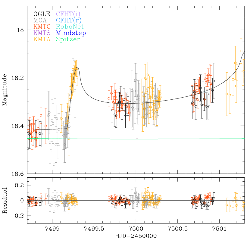
Figure 2: Further zoom of the lower-left panel of Figure 1, focusing on the data approaching and within the planetary caustic. The caustic entrance is well-defined by the KMTA and MOA data, with residuals that are consistent with the errors and that show no significant systematic trends.

Figures 1 and 2 show the light curve of all the data together with a best fitting model. Ignoring the model for the moment, the data show two clear isolated deviations from a smooth point-lens model: an irregular bump at HJD${}^{\prime}\sim 7500$ and an asymmetric peak at HJD${}^{\prime}\sim 7581$. Figure 1 shows the overall light curve together with two zooms featuring the regions around the these two anomalies, while Figure 2 shows a further zoom of the first anomaly. In addition, the data from the Spitzer spacecraft show a clear parallax effect, i.e., although the data are taken contemporaneously with the ground-based data, the light curves observed from the two locations are clearly different. The final model for the light curve must account for all of these effects: the two deviations from the point lens and the parallax effect seen from Spitzer.

The nature of the two deviations can be understood through the ground-based data alone. The two deviations could be caused by the same planet or, in principle, by two different companions to the host star. As we will show in Section 3.1, a single planet that explains the central caustic perturbation at HJD${}^{\prime}\sim 7581$ actually predicts the existence of the planetary caustic perturbation at HJD${}^{\prime}\sim 7500$ if the source trajectory is slightly curved. Such a curvature implies that we observe the orbital motion of the planet, and since orbital motion is partially degenerate with the parallax effect, in Section 3.2 we proceed with fitting the ground-based and Spitzer data together with both effects. In that section, we show that the prediction of the planetary caustic crossing is remarkably precise. Thus, for our final fits in Section 3.4, we model the light curve using a full Keplerian prescription for the orbit.

3.1 Ground-Based Model

The simplest explanation for the ground-based lightcurve is that both deviations could be due to a single companion. All companions that are sufficiently far from the Einstein ring produce two such sets of caustics, one set of outlying “planetary” caustic(s) and one “central” caustic. For wide-separation companions $(s>1)$, the second caustic lies directly on the binary axis. For close companions $(s<1)$ there are two caustics that are symmetric about this axis, but for low-mass companions, $(q\ll 1)$, these caustics lie close to the binary axis. Thus, a planetary companion can generate two well-separated deviations provided that the angle of the source trajectory relative to the binary axis satisfies $\alpha\sim 0$ or $\alpha\sim\pi$. If this is the true explanation, then the central caustic crossing should be consistent with a source traveling approximately along the binary axis of that caustic. If the central caustic crossing is not consistent with such a configuration, e.g., it would require a source traveling perpendicular to the binary axis, that would be evidence that the two deviations were due to two separate companions. To test whether there is any evidence for the latter hypothesis, we begin by excising the data from the isolated, first anomaly and fitting the rest of the ground-based light curve.

Such binary lens fits require a minimum of six parameters $(t_{0},u_{0},t_{\rm E},s,q,\alpha)$. The first three are the standard point-lens parameters (Paczyński, 1986), i.e., the time of lens-source closest approach, the impact parameter normalized to the angular Einstein radius $\theta_{\rm E}$, and the Einstein crossing time,

$$t_{\rm E}\equiv{\theta_{\rm E}\over\mu_{\rm rel}},$$ (4)

where ${\mbox{\boldmath$\mu$}}_{\rm rel}$ is the lens-source relative proper motion and $\mu_{\rm rel}=|{\mbox{\boldmath$\mu$}}_{\rm rel}|$. While for point lenses the natural reference point for $(t_{0},u_{0})$ is the (single) lens, for binary lenses it must be specified. We choose the so-called center of magnification (Dong et al., 2006, 2009). The remaining three parameters are the companion-star separation $s$ (normalized to $\theta_{\rm E}$), their mass ratio $q$, and the angle $\alpha$ of their orientation on the sky relative to ${\mbox{\boldmath$\mu$}}_{\rm rel}$. If the source comes close to or passes over the caustics, then one also needs to specify $\rho\equiv\theta_{*}/\theta_{\rm E}$, where $\theta_{*}$ is the source angular radius. We note that for $s<1$, the center of magnification is conveniently the same as the center of mass.

We model the light curve using inverse ray shooting (Kayser et al., 1986; Schneider & Weiss, 1988; Wambsganss, 1997) when the source is close to a caustic and multipole approximations (Pejcha & Heyrovský, 2009; Gould, 2008) otherwise. We initially consider an $(s,q,\alpha)$ grid of starting points for Markov Chain Monte Carlo (MCMC) searches, with the remaining parameters starting at values consistent with a point-lens model. Then $(s,q)$ are held fixed while the remaining parameters are allowed to vary in the chain. We then start new chains at each of the local minima in the $(s,q)$ $\chi^{2}$ surface, with all parameters allowed to vary.

We find the light curve excluding the early caustic crossing data can be explained by a planet with parameters:

$$(s,q,\alpha)=(0.60,0.016,-0.01).$$ (5)

As expected for a light curve generated by a single, low-mass companion, $\alpha$ is indeed close to zero. For such central-caustic events, we usually expect two solutions related by the well-known close-wide $(s\leftrightarrow s^{-1})$ degeneracy (Griest & Safizadeh, 1998; Dominik, 1999). Thus, we might also expect a second solution with parameters $(s,q,\alpha)=(1.67,0.016,-0.01)$. However, although the central caustics of both the $s<1$ and $s>1$ solutions are quite similar, the planetary caustic lies on the opposite side of the host as the planet for $s<1$ and on the same side for $s>1$. As a result, because $\alpha\sim 0$, the $s>1$ solution would produce a large planetary caustic crossing after the central caustic crossing, which we do not observe. Therefore, the $s<1$ solution is the only one that can explain the light curve.

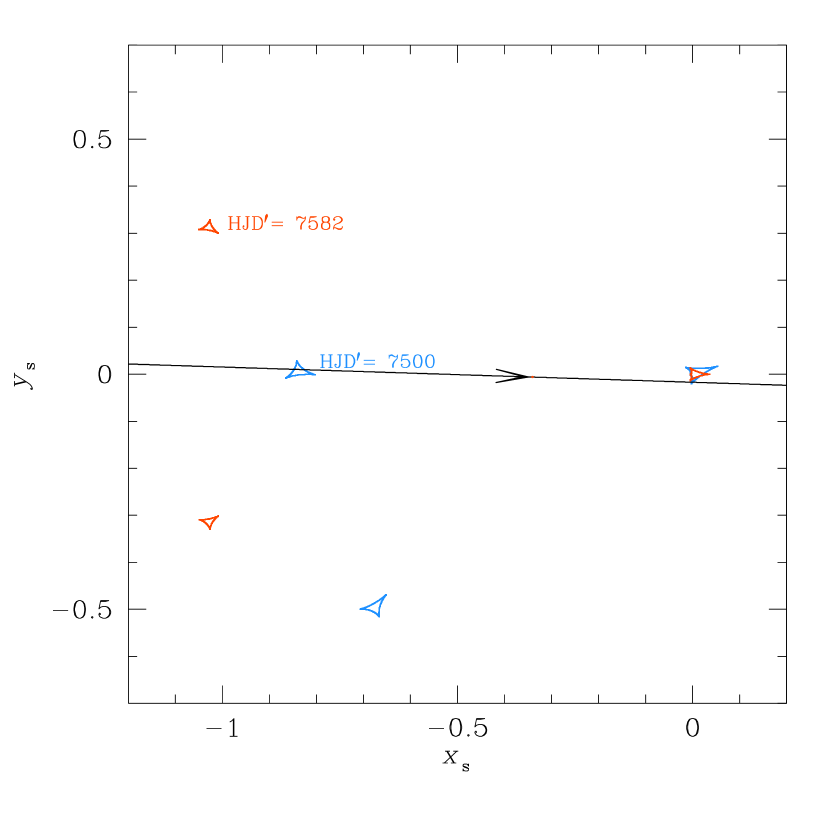
Figure 3: Geometry of the source and lens system based on ground-based data modeled with linearized orbital motion. The caustic structure is shown at two epochs, HJD${}^{\prime}=7500$ (blue) and 7582 (red) when, according to Figure 1, the source has just entered the planetary caustic and just passed the central caustic, respectively. A model that failed to include orbital motion and whose trajectory angle $\alpha$ was determined solely by modeling the source passage over the central caustic, would miss the (red) caustics.

Nevertheless, at first sight it does not appear that the $s<1$ solution can explain the planetary caustic crossing at HJD${}^{\prime}\sim 7500$. The $s<1$ caustic geometry is characterized by two caustics on opposite sides of this axis. For $(s,q)=(0.6,0.016)$, the angle between each caustic and the binary axis is $\phi\sim 16^{\circ}$ (see Equation (12)). Thus, given that the source trajectory is very close to the planet-star axis ($|\alpha|\ll 1$), it would appear that the source would pass between the two caustics (e.g., the source travels along the $x$-axis between the red caustics in Figure 3), whereas we clearly see in the data (Figure 1) that the source must pass over a caustic at $\sim 7500$.

However, this apparent contradiction can be resolved if the planet (and so caustics) have moved during the $\sim 80$ days between the times of the first perturbation and the second (when this geometry is determined). Naively, we expect motion of order $d\alpha/dt\sim 17^{\circ}/(80\,{\rm days})\sim 0.2^{\circ}{\rm day}^{-1}$. This kind of motion was indeed the resolution of the first such puzzle for MACHO-97-BLG-41 (Bennett et al., 1999; Albrow et al., 2000; Jung et al., 2013).

Hence, we conclude that the two perturbations are likely caused by a single companion, with the proviso that we must still check that the form of the planetary-caustic perturbation “predicted” by the central caustic crossing is consistent with the observed perturbation and that the amplitude of internal motion is consistent with a gravitationally bound system.

3.2 Linearized Orbital Motion and the Microlens Parallax

Given our basic understanding of the anomaly from the ground-based data, we can proceed with modeling the full dataset including Spitzer data. The ground-based modeling implies that the orbital motion effect plays a prominent role, so we allow for linearized motion of the lens system, i.e., we add two variables corresponding to the velocity of the lens projected onto the plane of the sky, $d\alpha/dt$ and $ds/dt$. Including the Spitzer data requires also including the parallax effect. The combination of these two effects implies the possibility of up to eight degenerate solutions: two solutions because with orbital motion the source can pass through either planetary caustic, multiplied by four solutions due to the well-known satellite parallax degeneracy (Refsdal, 1966; Gould, 1994b).

We begin by describing the color-magnitude diagram (CMD) analysis in Section 3.2.1 because it is used to derive the color-color relation needed for combining the Spitzer and ground-based data. Then, we give a qualitative evaluation of the Spitzer parallax in Section 3.2.2. In this section, we show that the color-color constraint plays an important role in measuring the parallax even though the Spitzer light curve partially captures the peak of the event. In Section 3.2.3, we present the full model of the event including linearized orbital motion and parallax. This modeling demonstrates that the orbital-motion parameters that are derived after excluding the $\pm 10\,$ days of data around the planetary caustic crossing are very similar to those derived from the full data set. Furthermore, the information from this restricted data set eliminates one of the two possible directions of orbital motion. Finally, in Section 3.3 we show that two of the parallax solutions can be eliminated by two separate arguments. First, they are inconsistant with Kepler K2 Campaign 9 microlensing observations. Second, they imply physical effects that are not observed. This leaves us with only two solutions, both of which carry the same physical implications for interpreting the light curve.

3.2.1 CMD and Spitzer-Ground Color-Color Relation

In order to derive the $VIL$ color-color relations needed to incorporate the Spitzer data, we must place the source on a CMD. We conduct this analysis by first using the OGLE $V/I$ CMD and then confirm and refine the result using $H$-band data from UKIRT.

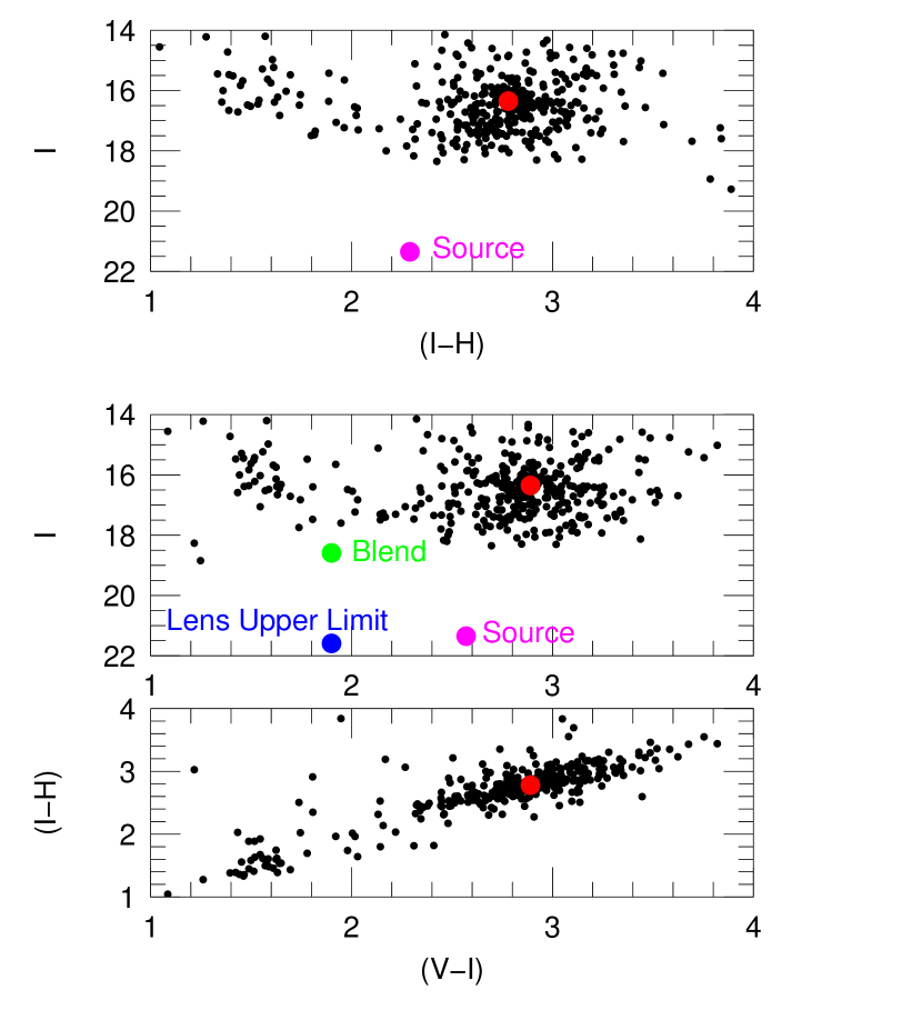
Figure 4: Instrumental color-magnitude diagrams in $(I-H,I)$ (top) and $(V-I,I)$ (middle), together with $VIH$ color-color diagram (bottom), which are derived by matching OGLE-IV instrumental $V$ and $I$ with UKIRT $H$ (aligned to 2MASS). The clump centroid is marked in red, while the source is marked in magenta. For the $(V-I,I)$ (middle) panel, the blended light is shown in green. Because the blend is displaced from the source by $0.5^{\prime\prime}$, only 6% of its light can be due to the lens. This flux upper limit shown, in blue (with arbitrary $(V-I)$ color), restricts the lens mass to $M_{L}\lesssim 1\,M_{\odot}$.

The middle panel of Figure 4 shows an instrumental CMD based on OGLE-IV data. The clump centroid is at $(V-I,I)_{\rm clump,O-IV}=(2.89,16.35)$. The source is shown at $(V-I,I)_{\rm s,O-IV}=(2.57\pm 0.06,21.35\pm 0.01)$, with the color derived by regression (i.e., independent of model) and the magnitude obtained from the (final) modeling. Also shown in this figure are two points related to the blended light, which are not relevant to the present discussion but will be important later. The key point here is that the source lies 0.32 mag blueward of the clump in the instrumental OGLE-IV system, which corresponds to 0.30 mag in the standard Johnson-Cousins system (Udalski et al., 2015b).

The top panel of Figure 4 shows an $I$ vs. $(I-H)$ CMD, which is formed by cross-matching OGLE-IV $I$-band to UKIRT $H$-band aperture photometry. The magnitude of the clump is the same as in the middle panel, $I_{\rm clump}=16.35\pm 0.05$. To ensure that the $(I-H)$ color of the clump is on the same system as the $(V-I)$ color, we make a $VIH$ color-color diagram in the lower panel based on cross-matched stars and then identify the intersection of the resulting track with the measured $(V-I)$ color to obtain $(I-H)_{\rm clump}=2.78\pm 0.02$. Also shown is the position of the source. Its magnitude is the same as in the middle panel. We determine $(I-H)_{s}=2.29\pm 0.03$ from a point lens model that excludes all data within 3 days of the anomalies. This permits a proper estimate of the error bars and is appropriate because the UKIRT data end 3.5 days before the anomaly at peak. Hence, the source lies 0.49 mag blueward of the clump in $(I-H)$. To derive the inferred offset in $(V-I)$ we consult the color-color relations of Bessell & Brett (1988). We adopt $(V-I)_{0,\rm clump}=1.08$ from Bensby et al. (2013), which implies $(I-H)_{0,\rm clump}=1.32$ based on Table III of Bessell & Brett (1988), and hence $(I-H)_{0,\rm s}=0.83\pm 0.03$. Then using Table II of Bessell & Brett (1988), we obtain $(V-I)_{0,\rm s}=0.75\pm 0.03$, i.e., 0.33 mag blueward of the clump. (Note that while we made specific use of the color of the clump in this calculation, the final result, i.e., the offset from the clump in $(V-I)$, is basically independent of the choice of clump color.)  Thus, the results of the two determinations are consistent. Although the formal error of the $I/H$-based determination is smaller than the one derived from OGLE-IV $V/I$ data, there are more steps. Hence we assign equal weight to the two determinations and adopt $(V-I)_{0}=0.77\pm 0.04$.

To infer the $I-L$ source color from the measured $(V-I)_{\rm s,O-IV}=2.57$, we employ the method of Shvartzvald et al. (2017b). In brief, this approach applies the $VIL$ color-color relations of Bessell & Brett (1988) to a $VIL$ cross-matched catalog of giant stars to derive an offset (including both instrumental zero point and extinction) between the intrinsic and observed $(I-L)$ color. Note that in this approach, explicit account is taken of the fact that the source is a dwarf while the calibrating stars are giants. We thereby derive $(I-L)_{s}=1.82\pm 0.06$. where here $L$ is the Spitzer instrumental magnitude.

From the CMD, we can also derive the angular source size $\theta_{*}$ (required to determine the Einstein radius $\theta_{\rm E}=\theta_{*}/\rho$). We adopt a dereddened clump magnitude $I_{0,\rm clump}=14.35$ (Nataf et al., 2013). Using this and the measurements reported above, we derive $[(V-I),I]_{0,s}=(0.77\pm 0.04,19.35\pm 0.05)$. Using the $VIK$ color-color relations of Bessell & Brett (1988) and the color/surface-brightness relations of Kervella et al. (2004), this yields (e.g, Yoo et al. 2004)

$$\theta_{*}=(0.455\pm 0.030)\,\mu{\rm as}.$$ (6)

where the error is dominated by scatter in the surface brightness at fixed color (as estimated from the scatter of spectroscopic color at fixed photometric color, Bensby et al. 2013). By combining this with $\rho$ measured from the final model (Section 3.4), we derive,

$$\theta_{\rm E}={\theta_{*}\over\rho}=(0.49\pm 0.04)\,{\rm mas}$$ (7)

3.2.2 Spitzer Parallax

Heuristically, space-based microlens parallaxes are derived from the difference in $(t_{0},u_{0})$ as seen from observers on Earth and in space, separated in projection by ${\bf D}_{\perp}$ (Refsdal, 1966; Gould, 1994b). The vector microlens parallax ${\mbox{\boldmath$\pi$}}_{\rm E}$ is defined (Gould, 1992, 2000; Gould & Horne, 2013)

$${\mbox{\boldmath$\pi$}}_{\rm E}\equiv{\pi_{\rm rel}\over\theta_{\rm E}}{{\mbox{\boldmath$\mu$}}_{\rm rel}\over\mu_{\rm rel}}.$$ (8)

Observers separated by ${\bf D}_{\perp}$ will detect lens-source separations in the Einstein ring $\Delta{\bf u}\equiv(\Delta\tau,\Delta\beta)=D_{\perp}{\mbox{\boldmath$\pi$}}_{\rm E}/{\rm AU}$, where

$$\Delta\tau\equiv{t_{0,\rm sat}-t_{0,\oplus}\over t_{\rm E}},\qquad\Delta\beta\equiv u_{0,\rm sat}-u_{0,\oplus}$$ (9)

and where the subscripts indicate parameters as determined from the satellite and ground. Hence, from a series of such measurements (which of course are individually sensitive to the magnification and not to $(t_{0},u_{0})$ directly), one can infer the vector microlens parallax

$${\mbox{\boldmath$\pi$}}_{\rm E}={{\rm AU}\over D_{\perp}}(\Delta\tau,\Delta\beta_{\pm,\pm})$$ (10)

where $\Delta\beta$ is generally subject to a four-fold degeneracy

$$\Delta\beta_{\pm,\pm}=\pm|u_{0,\rm sat}|-\pm|u_{0,\oplus}|$$ (11)

due to the fact that in most cases microlensing is sensitive only to the absolute value of $u_{0}$ whereas $u_{0}$ is actually a signed quantity.

This heuristic picture is somewhat oversimplified because ${\bf D}_{\perp}$ is changing with time, which also means that $t_{\rm E}$ is not identical for the two observers. Hence, in practice, one fits directly for ${\mbox{\boldmath$\pi$}}_{\rm E}$, taking account of both the orbital motion of the satellite and Earth (and hence, automatically, the time variable ${\bf D}_{\perp}(t)$). Nevertheless, in most cases (including the present one), the changes in ${\bf D}_{\perp}$ are quite small, $|d{\bf D}_{\perp}/dt|\pi_{\rm E}t_{\rm E}/{\rm AU}\ll 1$, which means that this simplified picture yields a good understanding of the information flow.

This qualitative picture can be used to show that the color constraints play an important role in this event, despite the fact that the peak is nearly captured in the Spitzer observations. As can be seen from Figure 1, in this case Spitzer observations begin roughly at peak. In general, it is quite rare that Spitzer observes a full microlensing light curve. This is partly because the maximum observing window is only 38 days, but mainly because the events are only uploaded to Spitzer 3–9 days after they are recognized as interesting (Figure 1 of Udalski et al. 2015a), which is generally after they are well on their way toward peak. Yee et al. (2015b) argue that with color constraints, even a fragmentary lightcurve can give a good parallax measurement. In this case, we have much more than a fragment, but as we show below, including the color constraints leads to a much stronger constraint on the parallax measurement.

If, as in the present case for Spitzer data, the peak of the lightcurve is not very well defined, a free, five parameter $(t_{0},u_{0},t_{\rm E},f_{s},f_{b})$, point lens fit would not constrain these parameters very well. However, in a parallax fit, we effectively know $t_{\rm E}$, which we approximate here as identical to the ground, $t_{\rm E}=94\,$days. After applying this constraint on $t_{\rm E}$, fitting the Spitzer data alone yields $t_{0,\rm sat}=7579.5\pm 1.4\,$days and $u_{0,\rm sat}=0.059\pm 0.021$, which would lead to a parallax error of $\sigma(\pi_{\rm E})\sim 0.021\,{\rm AU}/D_{\perp}\sim 0.016$ and so a fractional parallax error of $\sigma(\pi_{\rm E})/\pi_{\rm E}\sim 40\%$ for the small-parallax solutions. Note that this would not imply that the parallax is “unmeasured”: the fact that the parallax is measured to be small ($\lesssim 0.06$ and with relatively small errors) would securely place the lens in or near the bulge, which is significant information on its location.

However, by including the color-constraint, we can reduce this uncertainty to $<10\%$, giving a solid measurement of the parallax. First, one should note that the above fit to the Spitzer light curve yields a Spitzer source flux of $f_{s}=0.22\pm 0.11$ (in the instrumental Spitzer flux system). On the one hand, this is perfectly consistent with the prediction based on the ground solution and the $VIL$ color-color relation $f_{s,Spitz}=0.245\pm 0.015$, which is an important check on possible systematic errors. On the other hand, the errors on the fit value of $f_{s,Spitz}$ are an order of magnitude larger than the one derived from the $VIL$ relation. This means that the color-color relation can significantly constrain the fit. Imposing this additional constraint, we then find $t_{0,\rm sat}=7579.3\pm 0.8\,$days and $u_{0,\rm sat}=0.0635\pm 0.0029$, substantially improving the constraints on $u_{0,\rm sat}$. This reduces the parallax error to about 6% for the $\Delta\beta_{++}$ and $\Delta\beta_{--}$ solutions and to about 4% for the $\Delta\beta_{+-}$ and $\Delta\beta_{-+}$ solutions. See Section 3.3.

3.2.3 Modeling Orbital Motion

We now proceed with a simultaneous, 11-geometric-parameter $(t_{0},u_{0},t_{\rm E},s_{0},q,\alpha_{0},\rho,\pi_{{\rm E},N},\pi_{{\rm E},E},ds/dt,d\alpha/dt)$ fit to the ground- and space-based data. The first nine parameters have been described above. The last two are a linearized parameterization of orbital motion, with $\alpha(t)\equiv\alpha_{0}+(d\alpha/dt)(t-t_{0})$, $s(t)\equiv s_{0}+(ds/dt)(t-t_{0})$.

As discussed above, we expect a total of eight solutions: four from the satellite parallax degeneracy (Equation (11)) and two from the two planetary caustics. However, we found to our surprise that only one direction of angular orbital motion was permitted for each of the four parallax-degenerate solutions, i.e., the source trajectory could pass through one of the planetary caustics but not the other. These solutions are given in Table 2.

To understand why only one direction of angular orbital motion is permitted, we stepped back and performed a series of tests. In the first test, we fit for the above 11 parameters but, as in Section 3.1, with the data surrounding the planetary perturbation at $t_{p}={\rm HJD}^{\prime}\sim 7500$ removed (specifically $7490<{\rm HJD}^{\prime}<7510$). That is, we removed the information that we had previously believed was responsible for the measurement of orbital motion. Thus, we are testing whether information from the immediate neighborhood of the planetary caustic is required to predict the time and position of the planetary caustic crossing.

From the light curve (Figure 1), we can see that the midpoint of the two caustic crossings of the planetary caustic is $t_{p}\sim 7500.375$. From the modeling with the full dataset, we know the $y$ location of the caustic $\eta_{c,0}$ (Han, 2006). Therefore, if the orbital motion is constrained by the restricted data set, it should predict a planetary caustic close to this location. We conduct this test in a rotated frame for clarity. For each MCMC sample in the fit to the restricted data set, we predict the position of the center of the planetary caustic, first in the unrotated frame according to Han (2006),

$$(\xi,\eta_{\pm})=\biggl{(}s-{1\over s},{\pm\sqrt{q}\over s}\biggl{[}{1\over\sqrt{1+s^{2}}}+\sqrt{1-s^{2}}\biggr{]}\biggr{)}.$$ (12)

We then rotate by an angle $\phi=d\alpha/dt(t_{p}-t_{0})$ to obtain $(\xi^{\prime},\eta^{\prime}_{\pm})$, and finally convert this result to the observational plane

$$(t_{x},t_{y})=(t_{0},0)+(\xi^{\prime},\eta^{\prime})t_{\rm E}$$ (13)

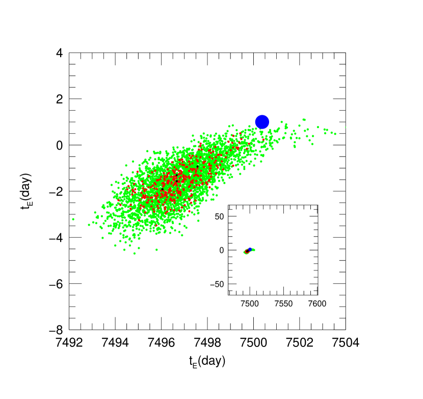
Figure 5: “Predicted” (small circles) versus “observed” (large blue circle) position of source crossing of planetary caustic within the Einstein ring. The predictions are from an MCMC chain created by fitting both ground-based and Spitzer data to a model with linearized orbital motion, but with the data points in the neighborhood of the observed planetary caustic crossing omitted. Points are colored by (black, red, green) for $\Delta\chi^{2}<(1,4,9)$. The abscissa of the prediction for each chain element is the time that the source should have crossed the center of the planetary caustic. The ordinate is that of the center of the caustic at this time, multiplied by $t_{\rm E}$. The abscissa of the “observed” position is the mid-time of the two caustic crossings shown in the lower-left panel of Figure 1. The ordinate is that of the source position at this time, multiplied by $t_{\rm E}$. Even without any “knowledge” of the source crossing, the model predicts its position very accurately. Inset shows zoom-out on the same scale as Figure 3.

The result is shown in Figure 5 along with the “observed” position of the caustic $(t_{x},t_{y})=(7500.375,1.0)$ derived from $(t_{p},\eta_{c,0})$.

There are two main points to note about this figure. The first is that the fit to the main light curve, primarily the central-caustic approach, alone measures the orbital motion parameters well enough to “predict” the position of the caustic to within a few $\sigma$. Second, this error bar is quite small, about 2 days in one direction (roughly aligned with time) and 0.5 days in the transverse direction. From the inset, which zooms out to the scale of Figure 3, one can see that the offset between the predicted and observed planetary-caustic crossing is tiny compared to the movement of the caustics that is illustrated in Figure 3.

This test demonstrates that the orbital motion can be determined quite precisely without data from the planetary caustic, but it does not in itself tell us what part of the light curve this information is coming from. In principle, it could be coming from the cusp approach at the peak of the light curve or it could be coming from subtle features in the light curve that lie 10 or more days from the planetary crossing and that are induced by the planetary caustic itself. Or, it could be some combination. In particular, one suspects that a significant amount of information must come from the central caustic because information from the “extended neighborhood” of the planetary caustic would not distinguish between the positive and negative values of $d\alpha/dt$ that are required for the source to cross, respectively, the lower and upper planetary caustics shown in Figure 3.

Hence, for our second test, we remove all data $7240<{\rm HJD}^{\prime}<7567$. Here we are directly testing what information is available from the central caustic region. As shown in Table 3 (bottom row), the measurement of the orbital parameters $ds/dt$ and $d\alpha/dt$ is quite crude compared to either the previous test or the full data set (first two rows). Nevertheless, $d\alpha/dt$ is detected at $4\,\sigma$. Moreover, in order for the direction of revolution to be in the opposite sense, so that the source would transit the other caustic in Figure 3, $d\alpha/dt$ should have the negative of its actual value, i.e., $d\alpha/dt\rightarrow+1.42$. Hence, the value measured after excluding all data $7240<{\rm HJD}^{\prime}<7567$ differs from the one required for opposite revolution by $7.4\,\sigma$. That is, it is the source passage by the central caustic that fixes the direction of the planet’s revolution about the host. Then as can be seen by comparison of the second and fifth lines of Table 3, it is the light curve in the general vicinity of the planetary caustic that permits precise prediction of the orbital motion when the data immediately surrounding the caustic are removed.

To further explore the origin of the orbital information, we show in Table 3 two additional cases, with data deleted in the intervals $7495<{\rm HJD}^{\prime}<7567$ and $7490<{\rm HJD}^{\prime}<7567$. Comparing the last three lines of Table 3, one sees that the lightcurve from more than 10 days before the crossing contributes greatly to the measument of transverse motion, and the following 5 days contributes even more. On the other hand, it is mostly the data after the crossing that contributes to the measurement of $ds/dt$.

A very important implication of Table 3 is that the orbital motion that is predicted based on the the subtle light curve features away from the planetary-caustic crossings yield accurate results. That is, of the eight hypothetical cases (2 parameters)$\times$(4 tests) the predictions of orbital motion are within $1\,\sigma$ of the true value for six cases, and at $2.0\sigma$ and $2.3\sigma$ in the remaining two. This provides evidence that such measurements are believable within their own errors in other events (i.e., the overwhelming majority) for which there is no way of confirming the results.

These results have important implications for microlensing observations with WFIRST (Spergel et al., 2013) and, potentially, Euclid (Penny et al., 2013) because their sun-angle constraints will very often restrict the light-curve coverage much more severely compared to those obtained from the ground.

3.3 Only The Two “Large Parallax” Solutions Are Allowed

The high precision of the two-parameter orbital motion measurement motivates us to attempt to model full Keplerian motion. However, before moving on to this added level of complexity, we first note that only two of the four solutions permitted by the parallax degeneracy are allowed. We present two distinct arguments, the first based on microlensing and the second based on physical considerations.

3.3.1 Degeneracy Breaking From Combined Kepler and Spitzer data

An important goal for the Spitzer microlensing program in 2016 was to combine Spitzer and Kepler data to break the 2-fold degeneracy between the two “large parallax” solutions (in which the source passes on opposite sides of the lens as seen from Earth and Spitzer) and the two “small parallax” solutions (in which they pass on the same side). The main idea for how this would work (Gould et al., 2015b) can be understood quite simply in the approximation that the projected positions of Earth, Kepler, and Spitzer are co-linear, i.e., ${\bf D}_{\perp,K2}=g{\bf D}_{\perp,Spitz}$, near the peak of the event, where $g$ is roughly constant over short time periods. Since all three bodies are in or very near the ecliptic, this approximation would be almost perfect for microlensing events in the ecliptic and is still quite good for the K2 field, which lies a few degrees from the ecliptic ($4^{\circ}$ for this event). In this case (as one may easily graph),

$$u_{0,k2}=gu_{0,Spitz}+(1-g)u_{0,\oplus}$$ (14)

and therefore

$${|u_{0,k2,\pm,\pm}|\over|u_{0,k2,\pm,\mp}|}={|g|u_{0,Spitz}|-(1-g)|u_{0,\oplus}||\over g|u_{0,Spitz}|+(1-g)|u_{0,\oplus}|}.$$ (15)

This formula can be more directly comprehended in the approximation (quite robust in the present case) that $A_{\rm max}\simeq|u_{0}|^{-1}$. Then,

$${A_{{\rm max},k2,\pm,\pm}\over A_{{\rm max},k2,\pm,\mp}}={gA_{{\rm max},\oplus}+(1-g)A_{{\rm max},Spitz}\over|gA_{{\rm max},\oplus}-(1-g)A_{{\rm max},Spitz}|}.$$ (16)

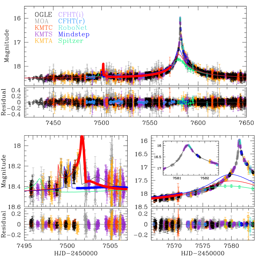
Figure 6: Similar to Figure 1 except that the predictions for Kepler “K2” observations (Henderson et al., 2016) are shown for the $(+,+)$ (red) and $(+,-)$ (blue) solutions. The time intervals when data were actually taken are shown in thick lines, while the times with no data are shown in thin lines. The large-parallax solutions [$(-,+)$ and $(+,-)$] predict a fainter peak from K2. See Equation (16). Unfortunately, K2 observations ended nine days before peak (lower right panel). Nevertheless, the two models predict radically different light curves for the planetary caustic crossing 80 days earlier. See text.

That is, the small parallax solutions ($(++)$ and $(--)$) will always yield higher peak magnifications for Kepler, unless either $u_{0,Spitz}=0$ or $u_{0,\oplus}=0$, in which case the “large” and “small” parallax solutions are equal anyway (Gould & Yee, 2012). In the present case, $g\simeq 5/8$ and $A_{{\rm max},\oplus}/A_{{\rm max},Spitz}\simeq 4$. Hence, Equation (16) predicts $A_{{\rm max},k2,\pm,\pm}/A_{{\rm max},k2,\pm,\mp}\simeq 23/17\sim 1.35$. This is quite close to the more precise value from a rigorous numerical model, which is illustrated in the main panel of Figure 6. (The offset between the two curves is less that the naive 0.33 mag because the curves are aligned to the ground-based light curve, which is heavily blended.)

Unfortunately, as also shown in Figure 6, there are no Kepler data over peak because the K2 C9 campaign ended nine days earlier. Moreover, as shown in the lower right panel, the large and small parallax models predict almost identical Kepler light curves in the region of the approach to the peak where there are data.

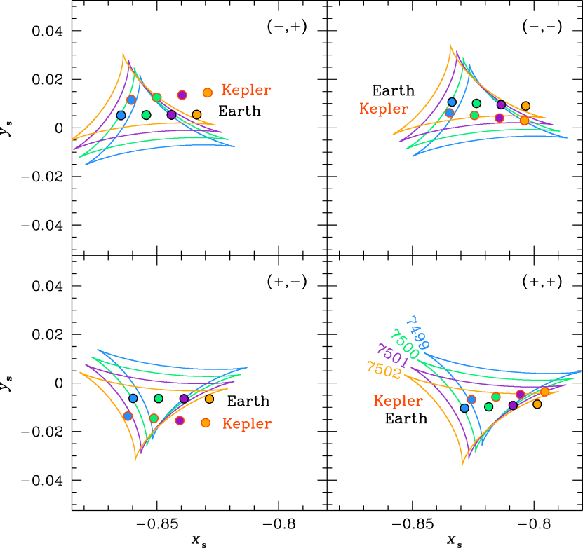
Figure 7: Planetary-caustic geometries for Kepler “K2” and Earth-based observations for the four solutions that are degenerate based on Earth-based and Spitzer data alone. For each day HJD${}^{\prime}=(7499,\ldots,7502)$, the caustic and the projected positions of the source as seen from Kepler and Earth are shown in the same color. In each of the four panels, the Earth-viewed source at a particular time is in a very similar position relative to the caustic, even though the caustic itself does not have the same position or orientation in the Einstein ring. This simply reflects that the model must match the ground-based data seen in Figures 1, 2, and 6. The vector offset between the Earth and Kepler positions is nearly constant within a given panel because their projected separation ${\bf D}_{\perp}$ barely changes during this interval. Because ${\mbox{\boldmath$\pi$}}_{\rm E}$ is quite precisely determined within each of the four solutions, the Kepler trajectory through the caustic is likewise well determined. But because of the opposite sign $\pi_{{\rm E},N}$ in, e.g., the $(-,+)$ and $(-,-)$ solutions, the ${\it Kepler}$-viewed source passes closer to the tip of the caustic in the first case (and so leaves the caustic before the first K2 data point at $\sim 7501$) whereas it passes closer to the base of the caustic in the second case (and so exits the caustic after the start of K2 observations). Hence the prediction of a dramatic difference for the “large parallax” (left panels) and “small parallax” (right panels) solutions is robust.

However, as shown in the lower left panel, the two models predict dramatically different light curves at the time of the first (planetary) caustic. While we have shown only one realization from the MCMC chain (the one with best $\chi^{2}$), we find that these predicted differences are extremely robust for all solutions with reasonable $\chi^{2}$. This robustness can be understood from Figure 7, which shows the source trajectories as seen from Earth and Kepler in the neighborhood of the planetary caustic for each of the four solutions.

The first point to note about these four panels is that while the caustic is not in the same place or same orientation in the Einstein ring (because the geometric parameters of these solutions are not exactly the same), the path of the source relative to the caustic as seen from Earth is extremely similar. This is simply because this path is directly constrained by the ground-based data that are shown in the lower left panel of Figures 1 and 6, and in the further zoom of this region shown in Figure 2. Second, if we look at each sub-figure separately, we see that the vector offset between the source positions seen from Earth and Kepler barely changes. This reflects that fact that over this short, three-day interval, ${\bf D}_{\perp,k2}(N,E)\simeq(-0.05,-0.13){\rm AU}$ is nearly constant.

The primary difference between the two upper panels is that for $(-,+)$, the source passes above the Earth trajectory as seen from Kepler, whereas for $(-,-)$ it passes below. Since the caustic is narrower toward the top, the source has already exited when the observations begin (magenta circle) for the $(-,+)$ case. Contrariwise, since the caustic widens toward its base, the earliest Kepler data are still inside the caustic for the $(-,-)$ case. Moreover, since the base of the caustic is “stronger” than the middle, the spike from the caustic exit is more pronounced than it is from Earth.

What is the reason for this opposite behavior? In both cases $u_{0,\oplus}<0$, meaning that, by definition (Figure 4 from Gould 2004), the source passes the lens on its left. Then, in the two cases, the source passes the lens as seen from Kepler on its left and right, respectively, implying that the source is displaced from Earth to opposite sides from the direction of motion.

A secondary effect is that Kepler is slightly leading Earth for $(-,+)$ and slightly trailing for $(-,-)$, which also contributes to the fact that the caustic exit does not occur “in time” for the start of the Kepler observations in the first case, but does in the second. These effects can be derived from the general formula for the Kepler-Earth offset relative to the direction of the source trajectory (following the formalism of Gould 2004),

$$(\Delta\tau,\Delta\beta)={(-{\mbox{\boldmath$\pi$}}_{\rm E}\cdot{\bf D}_{\perp},-{\mbox{\boldmath$\pi$}}_{\rm E}\times{\bf D}_{\perp})\over{\rm AU}}$$ (17)

However, since this is a secondary effect, we do not present details here.

Because microlensing fields are very crowded compared to the original Kepler field for which the camera was designed, there are usually several stars within a Kepler pixel that are much brighter than the microlensed source, even when it is magnified. This, combined with the not-quite regular 6.5-hour drift cycle in K2 pointing means that standard photometry routines cannot be applied to K2 microlensing data. Here we employ the algorithm of Huang et al. (2015) and Soares-Furtado et al. (2017), which was originally developed for other crowded-field applications and then further developed by Zhu et al. (2017b) for microlensing. We refer the reader to these papers for details of the method. However, an important point to emphasize is that the method requires detrending, which can partly or wholly remove long term features. Hence, for example, it could be problematic to apply it to the long, slow rise predicted for Kepler in the weeks before Campaign 9 ended on $\sim 7572.4$. Fortunately, as we have discussed, there is no possibility of distinguishing the models from this part of the light curve in any case.

Instead, we are only interested to determine whether there is a sharp “spike” in the K2 light curve shortly after the observations begin. Since detrending must be done separately on the two sections of K2 lightcurves (before and after the hiatus to download data beginning at ${\rm JD}^{\prime}=7527.4$), we restrict the detrending to before this date. We also restrict ${\rm JD}^{\prime}>7502.5$ to avoid the region of the light curve that could conceivably be impacted by the possible “spike”. In this interval, all microlensing models agree that the K2 light curve is essentially flat, so that it can be “modeled” as a constant. Note that since no microlensing model is required to construct this light curve, the specific modifications introduced by Zhu et al. (2017b) are not actually required for these reductions.

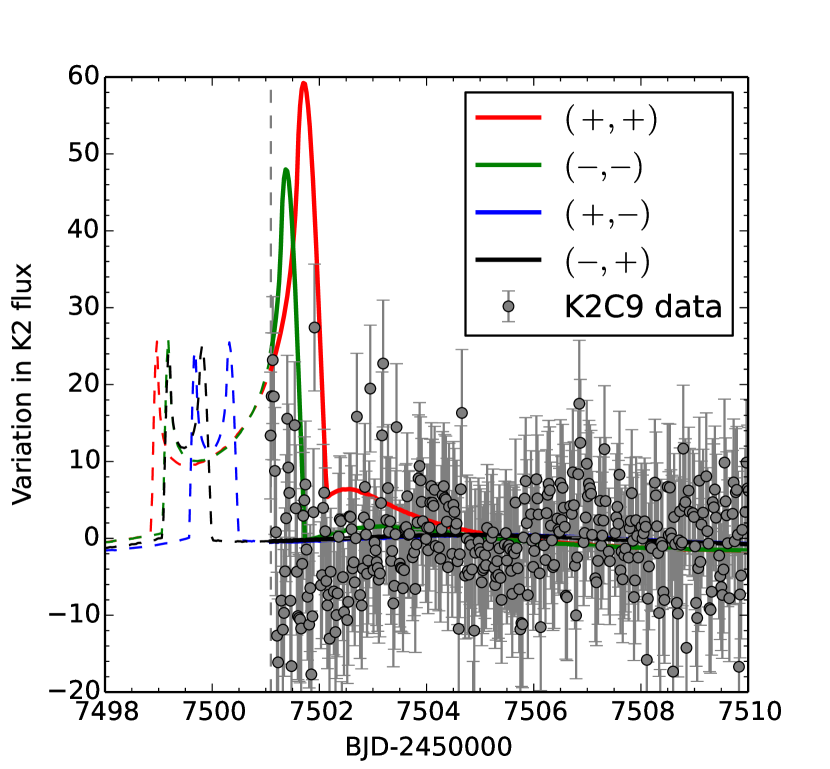
Figure 8: Observed (black points) K2 light curve compared to four microlens parallax model that would be degenerate based on ground-based and Spitzer data alone. The data do not show any indication of a spike at the predicted caustic exits of the two “small parallax” solutions [$(-,-)$ and $(+,+)$]. The times of these exits are very well predicted, as discussed in Section 3.3.1 and Figure 7. In order to determine the amplitude of these spikes, one must derive the source flux in the Kepler band $K_{p}$. This is done essentially by a $VIK_{p}$ color-color relation, with a small correction term based on the extinction, yielding $f_{s,Kepler}=6.1$. Hence, e.g., the red $(+,+)$ curve drops by $\Delta A=9.8$ magnification units between the peak and the post-caustic “baseline”. The uncertainty in this transformation is 0.1 mag, implying a $\sim 10\%$ uncertainty in the height of the spikes, which does not impact the robustness of the rejection of the “small parallax” models. The $(+,+)$ and $(+,-)$ solutions are shown on a magnitude scale in Figure 6, with the regions probed by K2 data (see this figure) highlighted in boldface.

Figure 8 shows the detrended K2 light curve together with the four otherwise-degenerate microlensing models. The “small parallax” models [$(+,+)$ and $(-,-)$] each predict a sharp spike due to a caustic exit shortly after the onset of the K2 C9 campaign, whereas the “large parallax” models do not. In order to transform the model magnification curves to predicted K2 light curve, one must determine the Kepler magnitude $K_{p}$ of the source. We first determine the calibrated $I$ and $V$ magnitudes of the source by aligning the OGLE-IV source magnitudes to the calibrated OGLE-III (Udalski et al., 2008; Szymanski et al., 2011) system $(V-I,I)=(2.44,21.47)$. We then incorporate extinction parameters from Nataf et al. (2013) and apply the transformations given in Zhu et al. (2017b) to find $K_{p}=23.03\pm 0.10$. That is, the model curves have a systematic scaling error of 10% flux. From Figure 8 it is clear that the K2 data are inconsistent with the “small parallax” models, even allowing for this 10% error in the scale of the models.

Of course, the entire argument given in this section depends on the model being correct within its stated errors. We mentioned above that all models that are consistent with the data yield extremely similar light curves in the neighborhood of the caustic, which, as we emphasized, is not at all surprising given that the source trajectory relative to the caustic is directly determined by the data.

In principle, there remains the question of whether the data themselves have systematics that would incorrectly constrain the model to this particular geometry. Figure 2 shows that this is unlikely because on the principal defining feature, the caustic entrance, the data (particularly KMTA) have errors ($\sim 0.05\,$mag) that are small compared to the compared to the caustic entrance “jump” ($\sim 0.25\,$mag). Nevertheless, given the apparent importance of these data to the final result, we conduct four tests that alter the data around the planetary caustic $(7490.5<{\rm HJD}^{\prime}<7510.5)$: 1) remove MOA data, 2) remove KMTA data, 3) bin both MOA and KMTA data, 4) remove both MOA and KMTA data. We find that the fit parameters change by $\ll 1\,\sigma$ when MOA data are removed and by $<1\,\sigma$ when KMTA data are removed. These first two tests essentially rule out that the result can be strongly influenced by systematics, since it is extremely unlikely that the systematics would be the same at observatories separated by thousands of km. Even when both data sets are removed, the results change by $\lesssim 1\,\sigma$. Binning the data also affects the results by $<1\,\sigma$.

It may seem somewhat surprising that even elimination of both MOA and KMTA do not prevent the model from precisely locating the planetary caustic given that these data sets alone probe the caustic entrance. However, the size, shape and orientation of the caustic are precisely specified by the parameters $[s(t_{c}),q,\alpha(t_{c})]$, which are well determined from the overall model. Here, $t_{c}=7500$ is the time of the planetary caustic. Given this, the facts that the OGLE and KMTC data probe the internal height of the caustic at two epochs, while the KMTS (and also KMTC) data define the post-caustic cusp approach, constrain the position of the caustic quite well.

We conclude that the analysis given in this section is robust against both statistical and systematic errors.

3.3.2 Degeneracy Breaking From Physical Constraints

Next we give a completely independent argument that essentially rules out the “small parallax” solutions. Almost by definition (Equation (11)), $|\Delta\beta_{\pm,\pm}|<|\Delta\beta_{\pm,\mp}|$, and therefore $|\pi_{{\rm E},{\pm,\pm}}|<|\pi_{{\rm E},{\pm,\mp}}|$. Hence, the masses $M=\theta_{\rm E}/\kappa\pi_{\rm E}$ for the $(+,+)$ and $(-,-)$ solutions are higher than the other two solutions. In the present case, they are higher by a factor $\sim 1.75$, which would put the primary at $M=1.60\pm 0.16\,M_{\odot}$. See Table 4.

There are two arguments against such a heavy lens. First, it would give off too much light. Second, given its almost certain location in the Galactic bulge, its main-sequence lifetime ($\lesssim 2\,$Gyr) would be too short given the typical range of ages of bulge stars. Both of these arguments implicitly assume that the host is not a neutron star, which we consider to be extremely unlikely given the complete absence of easily detectable massive companions like OGLE-2016-BLG-1190Lb at a few AU around pulsars. See Figure 1 of Martin et al. (2016) and note that while the black points have similar masses to OGLE-2016-BLG-1190Lb, they have semi-major axes $a\sim R_{\odot}$ and hence are likely to be stripped stars rather than planets and, in any case, not at $a\sim{\rm AU}$.

The blended light shown in Figure 4 $[(V-I),I]_{\rm b,O-IV}=(1.90,18.59)$ lies just 2.3 mag below the clump and is about 1 mag bluer than the clump. Hence, it would not be at all inconsistent with a roughly $1.6\,M_{\odot}$ star at the distance of the Galactic bulge. However, although the source star is intrinsically faint, its position can be determined with high precision when it is highly magnified, from which we determine that the light centroid of the blend is offset from the position of the blend by $0.5^{\prime\prime}$. By examining the best-seeing OGLE-IV baseline images, we find that the total light at the position of the source must be less than 13% of the blended light. Since (from the fit) $f_{s}/f_{b}=0.07$, the light due to the lens must be at least 3 mag fainter than blend, and hence 5.3 mag fainter than the clump. This is clearly inconsistent with a star in the bulge that is significantly more massive than the Sun.

In addition, the lens-source relative parallax for the $(+,+)$ and $(-,-)$ solutions is $\pi_{\rm rel}\simeq 20\,\mu{\rm as}$. The source-lens relative distance is given by $D_{LS}\equiv D_{S}-D_{L}=\pi_{\rm rel}D_{L}D_{S}/{\rm AU}\simeq 1.2\,{\rm kpc}$. This small separation, combined with the fact that the source color and magnitude are quite consistent with it being a bulge star, imply that the lens is heavily favored to lie in the bulge. The bulge is generally thought to be an old population. If this were strictly true, it would rule out such massive bulge lenses. However, Bensby et al. (2017) find that their sample of microlensed bulge dwarfs and subgiants has a few percent of stars with ages less than 2 Gyr. Thus, while this second argument against the $(+,+)$ and $(-,-)$ solutions is less compelling than the first argument, it does tend to confirm it.

3.4 Full Keplerian Orbital Solution

To investigate full Kepler solutions, we add two new parameters and transform the meaning of two previous parameters to obtain $(t_{0},u_{0},t_{\rm E},s,q,\alpha,\rho,\pi_{{\rm E},N},\pi_{{\rm E},E},ds_{\bot}/dt,d\alpha/dt,s_{\parallel},ds_{\parallel}/dt)$; we also specify the reference time $t_{\rm binary}=7582.16$. Here, the two triples $(s,0,s_{\parallel})$ and $[ds_{\bot}/dt,s(d\alpha/dt),ds_{\parallel}/dt]$ are, respectively, the instantaneous planet-star separation and relative velocity, in the coordinate frame defined by the planet-star axis on the sky, the direction within the plane of the sky that is perpendicular to this, and the direction into the plane of the sky. The units are Einstein radii and Einstein radii per year, so that to convert to physical units one should multiply by $D_{L}\theta_{\rm E}$. Of course, if these parameters are specified, together with the total mass of the system, one can determine the full orbit and hence the Kepler parameters.

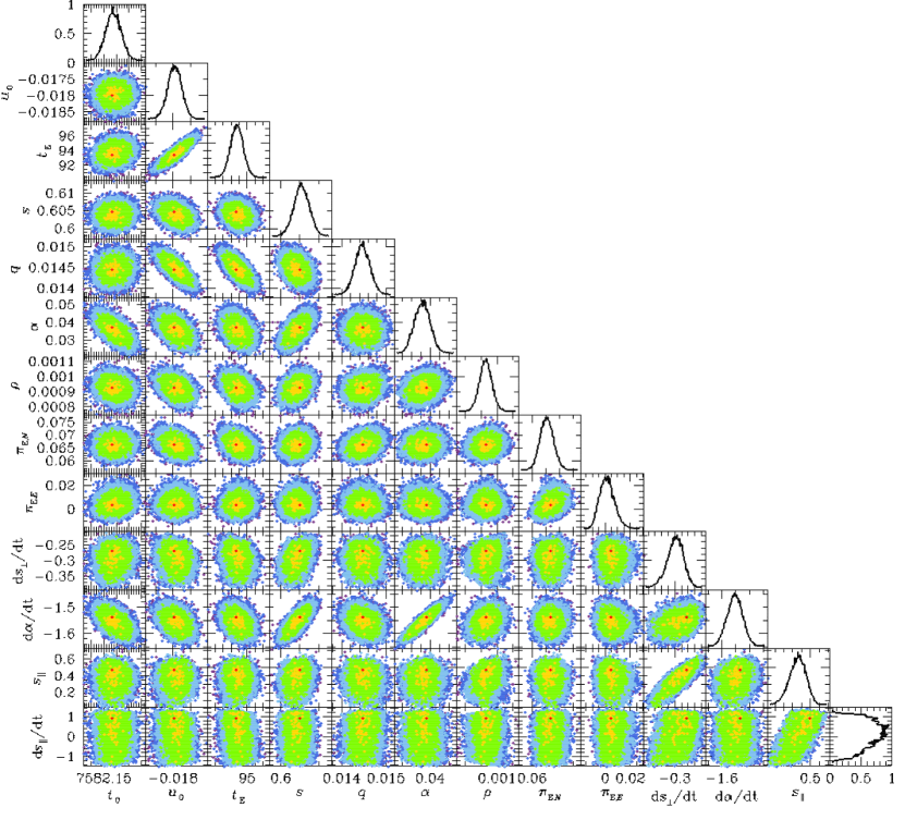
Figure 9: Scatter plots of pairs of all 13 microlensing parameters from the complete orbital solution for the $(-,+)$ minimum. The plots for the $(+,-)$ solution (which has a worse fit by $\Delta\chi^{2}=4$) look qualitatively similar. (Red, yellow, green, cyan) points are within $\Delta\chi^{2}<(1,4,9,16)$ of the minimum. All parameters are relatively well-constrained except $ds_{\parallel}/dt$, i.e., the line of sight velocity of the planet in units of Einstein radii per year.

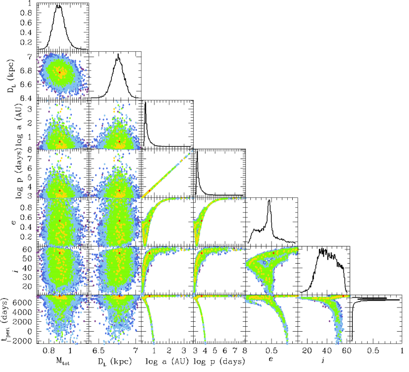
Figure 10: Scatter plots of pairs of 6 Kepler parameters that are derived from the chain of the complete orbital solution for the $(-,+)$ minimum. (Red, yellow, green, cyan) points are within $\Delta\chi^{2}<(1,4,9,16)$ of the minimum. The Kepler parameters period $P$, eccentricity $e$, inclination $i$, and time of periastron $t_{\rm peri}$ are confined to an essentially one-dimensional sub-space.

Skowron et al. (2011) discusses the transformations from microlensing parameters to Kepler parameters in detail. For each MCMC sample, one determines $\theta_{*}$ from the value of $f_{s}$ and the model-independent color. Then from the value of $\rho$, one obtains $\theta_{\rm E}=\theta_{*}/\rho$. Then from the value of the parallax ${\mbox{\boldmath$\pi$}}_{\rm E}$, one determines $M=\theta_{\rm E}/\kappa\pi_{\rm E}$ and $\pi_{\rm rel}=\theta_{\rm E}\pi_{\rm E}$. In order convert the position and velocity parameters into physical separations and velocities, one still needs $D_{L}={\rm AU}/(\pi_{\rm rel}+\pi_{s})$ where $\pi_{s}$ is the source parallax. For this we adopt $D_{s}=8.7\,{\rm kpc}$, as discussed below in Section 4. We report the microlens parameters for the two remaining solutions in Table 5 and show the MCMC sampling of parameters for one of these solutions in Figure 9. We also show the transformation of this sampling to the key Kepler parameters in Figure 10.

Figures 9 and 10 show that while the microlens parameters exhibit well-behaved, relatively compact distributions, the Kepler parameters follow complex one-dimensional structures. This is probably due primarily to the fact that one of the two new parameters $s_{\parallel}$ is relatively well constrained, while the other $ds_{\parallel}/dt$ is fairly poorly constrained. As a result, some of the Kepler parameters are also poorly constrained. In particular, unfortunately, it is not possible to strongly constrain the eccentricity, which would have been a first for microlensing. Nevertheless, we note that OGLE-2016-BLG-1190Lb has the best constrained orbit of any microlensing planet yet detected.

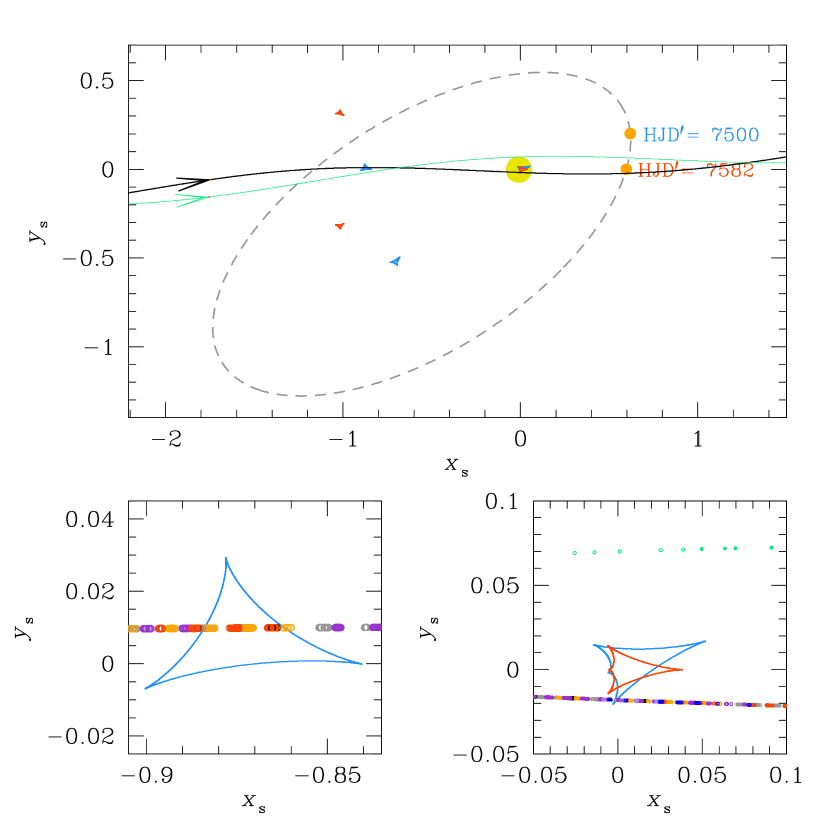
Figure 11: Geometries of the source and lens system for the $(-,+)$ solution. The dashed gray line shows the planet’s orbit for the best-fit model with its position at the times of the two caustic crossings shown by orange dots. However, the parameters such as the orbital inclination and eccentricity have large uncertainties, and thus there are many possible orbital geometries. The caustic structure at the first of these epochs is shown in blue and at the second in red. The trajectories of the source position through the Einstein ring as seen from Spitzer and Earth are shown in green and black, respectively. Their “waviness” reflects the heliocentric orbital motion of these two observatories. Epochs of observations are shown by small circles, using same color scheme as in Figure 1. The yellow circle at the position $(X_{s},Y_{s})=(0,0)$ shows the position of lens star. The corresponding $(+,-)$ diagram looks essentially identical, but inverted with respect to the $x$-axis.

Figure 11 shows the geometry of the source and lens system together. The dashed black line shows the planet’s orbit, with its position at the times of the two caustic crossings shown by orange dots. The caustic structure at the first of these epochs is shown in blue and at the second in red. The trajectories of the source position through the Einstein ring as seen from Spitzer and Earth are shown in green and black respectively. The curvature in these two trajectories reflects the orbital motion of these two observatories about the Sun.

Table 6 summarizes the evolution of models developed in this paper. The penultimate column gives the change in $\chi^{2}$ relative to the previous model, for the set of observatories specified in the final column. The “standard model” (no higher order effects) was not presented here in the interest of space and is shown for reference in order to emphasize the enormous improvement in $\chi^{2}$ by introducing two orbital parameters. We introduced parallax at the same time that we included Sptizer data. The fact that $\chi^{2}_{\rm gr}$ decreases by $\Delta\chi^{2}_{\rm gr}=10.6$ means that the ground-based data corroborate the much more precise Spitzer parallax measurement at this level. The final $\Delta\chi^{2}=9.6$ improvement when full orbital motion is included may seem rather modest, and within conventional reasoning on this subject it might even be questioned whether these two extra parameters have been “detected”. However, as pointed out by Han et al. (2016), since binaries are known a priori to have Keplerian orbits, the only justification required for introducing additional parameters is that they can be measured more precisely than they are known a priori.

4 Physical Characteristics

The physical parameters derived from the full orbital solutions are given in Table 7. As discussed in Section 3.3, the blended light in the CMD (Figure 4) provides a constraint on the lens mass, independent of the modeling. The light superposed on the source (including the lens and possibly other stars) is at least 5.3 mag below the clump, which excludes lenses that are significantly more massive than the Sun. As discussed there, this essentially rules out the $(+,+)$ and $(-,-)$ solutions. For the $(+,-)$ and $(-,+)$ solutions, since very few of the MCMC samples exceed this mass limit, we do not bother to impose this constraint. However, we note that given the mass measurements reported in Table 7, together with the faintness of the source shown in Figure 4, the lens should be easily detectable in high resolution images, a point to which we will return below.

The main focus of interest is the mass of the companion and the distance of the system,

$$M_{2}=13.4\pm 0.9\,M_{J};\qquad D_{L}=6.8\pm 0.1\,{\rm kpc}.$$ (18)

The mass is at the edge of the conventional planetary range, i.e., a massive super-Jupiter, very close to the deuterium limit that conventionally separates “brown dwarfs” from “planets”.

As discussed by Calchi Novati et al. (2015a), what is actually measured precisely in microlensing events is $\pi_{\rm rel}=\theta_{\rm E}\pi_{\rm E}$ rather than $D_{L}={\rm AU}(\pi_{\rm rel}+\pi_{s})^{-1}$ because the precise value of $D_{s}$ (and so $\pi_{s}={\rm AU}/D_{S}$) is not known. The uncertainty in $\pi_{s}$ becomes particularly important for lenses in and near the bulge because it dominates the error in $D_{L}$. For example, in the present case $\pi_{\rm rel}=33\pm 3\,\mu{\rm as}$, whereas a 7% error in $D_{S}$ would yield an error in $\pi_{s}$ almost three times larger than this.

For this reason, Calchi Novati et al. (2015a), introduced a deterministic tranformation of $\pi_{\rm rel}$ that could be used in statistical studies of Spitzer microlensing events, $D_{8.3}$ which can be evaluted in the present case

$$D_{8.3}\equiv{{\rm kpc}\over\pi_{\rm rel}/{\rm mas}+1/8.3}=6.54\pm 0.13\,{\rm kpc}.$$ (19)

This formulation has the advantage that it is symmetric with respect to nearby and distant lenses. That is, for lenses near the Sun, $D_{L}\rightarrow D_{8.3}$ while for lenses near the source, $D_{LS}\equiv D_{S}-D_{L}\rightarrow 8.3\,{\rm kpc}-D_{8.3}$. Hence, because $D_{8.3}$ is more precisely determined than $D_{L}$, particularly for lenses in and near the bulge, it is more suitable for statistical studies and for comparison of different events. To enable such comparisons, we always use 8.3 (kpc) in the denominator of Equation (19) rather than the best estimate of the source distance. However, there is very little cost to this approximation in terms of its impact on the quantity of physical interest for near bulge lenses, $D_{LS}$, which is approximated by $D_{LS,8.3}\equiv 8.3\,{\rm kpc}-D_{8.3}$ For example, in the present case

$${D_{LS,8.7}-D_{LS,8.3}\over D_{LS,8.7}}\rightarrow{1.91\,{\rm kpc}-1.76\,{\rm kpc}\over 1.91\,{\rm kpc}}=8\%.$$ (20)

We note that the distance shown in Equation (18) adopts the same uncertainty as Equation (19) and neglects the uncertainty due to the source distance. In this case, we have derived the above lens distance by fixing the source distance at $8.7\,{\rm kpc}$, i.e., about $0.9\,{\rm kpc}$ behind the center of the “bulge” (really, “bar”) toward this line of sight. We have chosen this distance as typical because, as we argue just below, the lens and source are both likely to lie in the Galactic bar.

Both the measured values of $\pi_{\rm rel}$ and $\mu_{\rm rel}$ indicate that the most probable configuration is that the lens and source are roughly equally displaced from the center of the bar. The measured value of $\pi_{\rm rel}$ leads to an inferred lens-source separation $D_{LS}=D_{L}D_{S}\pi_{\rm rel}/{\rm AU}=2.1\pm 0.2\,{\rm kpc}$. This is consistent with the lens being in the bar, but it does not by itself argue strongly for such an interpretation. The lens could also lie $\sim 2\,{\rm kpc}$ in the front of the bar, in the Galactic disk. However, in this case, we would expect the lens-source relative proper motion to be substantially greater than the one that is measured: $\mu=1.9\,{\rm mas}\,{\rm yr}^{-1}$. This small value of the relative proper motion is more consistent with a source and lens drawn from kinematically related populations of stars. Thus, we tentatively conclude that this very massive super-Jupiter companion to a G dwarf is in the bar/bulge and adopt a source distance $D_{s}=8.7$ kpc.

However, at this stage, a disk lens cannot be ruled out. In particular, if the source happened to be moving at $\sim 5\,{\rm mas}\,{\rm yr}^{-1}$ in the direction of Galactic rotation, then the inferred motion for the lens (based on the observed ${\mbox{\boldmath$\mu$}}=\mu({\mbox{\boldmath$\pi$}}_{\rm E}/\pi_{\rm E}$)) would be quite consistent with disk kinematics.

Because the lens and source are almost certainly detectable in high resolution imaging (whether space-based or ground-based), this question about the lens kinematics can be resolved within a few years. Under most circumstances, such followup observations require that the source-lens relative motion be measured (which could take quite some time given their low relative proper motion). In the present case, the relative motion is small meaning that the source and lens will remain unresolved for many years, but we can still measure their joint proper motion relative to the stellar background. Two measurements separated by two years should be sufficient to determine this joint motion relative to the frame of field stars. The absolute motion of this frame can then be determined from Gaia data. Since the lens and source are hardly moving relative to one another, this should indicate the kinematics of the lens star. Finally, one can make a final correction from the observed, joint proper motion to the lens proper motion based on the well measured magnitude and direction of the lens-source relative proper motion (from the microlens solution) together with the ratio of the source flux (also from the microlens solution) to the total flux (from the high-resolution data themselves).

To aid in such future observations we report the $(I-H)_{s}$ color of the source, as described in Section 3.2.1 and also the $H_{s}$ magnitude of the best-fit model

$$(I_{\rm ogle}-H_{\rm 2mass})_{s}=2.29\pm 0.03;\qquad H_{s}=19.06\pm 0.04$$ (21)

5 Assignation to Spitzer Parallax Sample

The Galactic distribution of planets experiment must be carried out strictly in accord with the protocols specified by Yee et al. (2015b), which were designed to maintain an unbiased sample. Because OGLE-2016-BLG-1190 was selected for Spitzer observations on the basis of the planetary anomaly observed at $\sim 7500$, it would naively appear that this planet cannot be included in a sample that must be unbiased to planets. However, Yee et al. (2015b) anticipated just such a situation (in which the planetary anomaly occurs early in the light curve) and so laid out specific criteria under which such planets may be included while still maintaining the objectivity of the sample.

Yee et al. (2015b) specify several ways an event may be selected for Spitzer observations, two of which are relevant here. The first is following pre-specified “objective” criteria under which planets found during any part of the event can be included in the sample. If an event meets certain purely objective criteria, then it must be observed by Spitzer at a specified minimum cadence (usually once per day). Observations can only be stopped according to specified conditions. Since there is no human element involved in event selections of this type, any planets and planet sensitivity automatically enter the unbiased sample. However, Spitzer time is extremely limited and “objective” selection places a large and rigidly enforced burden on this time, so the “objective” criteria must be set conservatively.

Therefore Yee et al. (2015b) also specify the possibility of “subjective” selection, which can be made for any reason deemed appropriate by the team. In this case, only planets (and planet sensitivity) from data not available to the team at the time of their decision can be included in the sample. Specifically, if a planet (or a simulated planet used to evaluate planet sensitivity) gives rise to a deviation from a point-lens model in such available data that exceeds $\Delta\chi^{2}=10$, then it must be excluded. This effectively removes not only “known” planets but also “unconsciously suspected” planets. The cadence and conditions for stopping subjectively alerted events must be specified at the time they are publicly announced.

Although “subjective” selection has the obvious disadvantage that only planets discovered after the selection can be included in the sample, there are several advantages to this type of selection. Many of these advantages derive from the fact that Spitzer targets can only be uploaded to the spacecraft once per week and must be finalized $\gtrsim 3$ days before observations begin. First, an event may never become objective and yet still be a good candidate. For example, if it is short timescale and peaks in the center of the Spitzer observing “week,” it may still be too faint to meet the “objective” criteria when the decision to observe must be made and again may be too faint the following week. Second, the team may select an event “subjectively” a week or two before it meets the “objective” criteria. In that case, Spitzer observations start a week or two earlier, improving the measurement of the parallax. Likewise, the team may specify a higher Spitzer cadence for a “subjectively” selected event, resulting in more observations and a better parallax.

Yee et al. (2015b) also specify how to classify an event that may be selected multiple ways, such as a “subjective” event that later meets the “objective” criteria. From the perspective of measuring a planet frequency, “objectively” selected events are clearly better because then planets from the entire light curve can be included. However, from the perspective of measuring the Galactic distribution of planets, an event is worthless if the parallax is not measured. Thus, Yee et al. (2015b) state that the “objective” classification takes precedence as long as the parallax is “adequately” measured from the subset of the data that would have been taken in response to an “objective” selection, i.e., after removing any data taken before the “objective” observations would start and thinning the data to the “objective” cadence. If the parallax is not “adequately” measured from this subset of the data, then the event reverts to being “subjectively” selected and, consequently, all planets detectable in data available prior to the selection date are excluded. However, if an event is determined to be “objective” based on these criteria, all Spitzer data can be used to characterize the lens.

Yee et al. (2015b) do not specify what precision is required for an “adequate” parallax, but this was discussed in Zhu et al. (2017a). They established a condition

$$\sigma(D_{8.3})<1.4\,{\rm kpc}.$$ (22)

We note that Calchi Novati et al. (2015a) introduced $D_{8.3}$ because $\pi_{\rm rel}$ is more reliably measured than $D_{L}$ and because this quantity gives symmetric information on the distance between the observer and lens for nearby lenses and between the source and lens for distant lenses.

OGLE-2016-BLG-1190 was clearly initially selected “subjectively,” and under those criteria, the planet could not be included. In Section 5.1, we show that this event actually met the “objective” criteria. Then, in Section 5.2, we examine whether or not the data taken in response to the “objective” selection meet the Zhu et al. (2017a) criterion (Equation 22) for an adequately measured parallax.

5.1 Yee et al. (2015) Protocols: Is the Event Objective?

As discussed in Section 2.2, OGLE-2016-BLG-1190 was initially selected on 1 July 2016 solely because the pre-alert light curve contained a candidate planetary anomaly. A check at the time of the initial upload to Spitzer (4 July 2016) showed that it did not meet objective criteria. As we now show, however, at the upload the following week on Monday 11 July 2016, the event did meet the objective criteria for rising events (B1–5) of Yee et al. (2015b). We note that while the Spitzer team does make some effort to determine which already-selected events have become “objective”, this is not carried out uniformly, nor is it required by the Yee et al. (2015b) protocols. No such effort was made for OGLE-2016-BLG-1190, so we are doing it here for the first time.

There are two sets of “objective” criteria: “falling” criteria that take into account the model fit and “rising” criteria based almost entirely on model-independent observables. The reason for the distinction is that the model parameters generally remain uncertain until after an event has peaked. For rising events, there is only one model-dependent criterion, i.e., that according to the best fit model, the event has not yet peaked or is less than 2 days past peak. Here the idea is that either the event has already peaked, in which case there is a good model for when that peak occurred, or it has not peaked in which case no plausible model will say that it peaked more than 2 days previously. On 11 July, OGLE-2016-BLG-1190 was clearly pre-peak and therefore should be judged under the “rising” criteria.

For an event to meet the “rising” criteria, it must be in a relatively high cadence OGLE or KMTNet field, which as described in Section 2.1 is clearly satisfied. Then, there are three flux criteria that must be satisfied. First $I_{\rm now}<17.5$, second $I_{\rm now}<I_{\rm base}-0.3$, and third $I_{\rm now}<16.3+0.93A_{I}$, where $A_{I}$ is the $I$-band extinction toward this field. Since $A_{I}>1.3$ and $I_{\rm base}<17.8$, the operative condition is $I_{\rm now}<17.5$.

To assess whether or not OGLE-2016-BLG-1190 met these flux criteria, we must be careful to make use of the data only as they were available to the team at the time of the final decision, UT 13:30 11 July (HJD${}^{\prime}=7581.06$). This means not only truncating the data at that date, but also using the versions of the data sets that were available and verifying that these were in fact available. MOA data are accessible in real-time while the OGLE data are generally delayed by of order 12 hours. We check that the last such OGLE data point was posted at HJD${}^{\prime}=7580.04$. In addition, the magnified-source flux derived from OGLE data that were available online at that time are fainter than the re-reduced data used in the analysis (Section 3) by an average of $\sim 0.23$ mag. This is because the online data were obtained using a catalog star whose position was displaced by $0.5^{\prime\prime}$ from the true source, as noted in Section 3.3. Since the OGLE scale is used by the Spitzer team for the flux determinations, we must use the online OGLE data (rather than the re-reduced data) to assess whether or not OGLE-2016-BLG-1190 met the flux criteria.

We fit the online OGLE and MOA data HJD${}^{\prime}<7581.06$ to a point-lens model (note that no OGLE data were taken between 7579.762 and 7581.719). This fit shows that the event reached $I=17.5$ on the online-OGLE scale about 1.65 days before the upload deadline. This means that the MOA data points taken beginning 1.3 days before this deadline, which could be aligned to the OGLE scale, were already above the threshold, leaving no doubt that the event became objective well in advance of the upload time.

5.2 Zhu et al. (2017) Protocols: Is the Parallax Measured?

The parallax is clearly measured from the analysis of the full dataset (Section 3). We now must determine whether or not the parallax is “objectively” measured and meets the Zhu et al. (2017a) criterion in Equation (22). First, we can only include the Spitzer data starting at 7585.98, the date objective Spitzer observations would have begun. Second, we must determine whether it would have met the Zhu et al. (2017a) criterion if it had been a point-lens event. This is because planetary events contain two types of information that preferentially enable them to meet this criterion, which point-lens events generally lack, and if we did not remove this information prior to testing against Equation (22), we would bias the sample toward planets. First, planetary events can contain additional ground-based, annual-parallax information due to sharp features in the light curve. This was first clearly noted by Muraki et al. (2011) for MOA-2009-BLG-266. Second, planetary events lead to measurement of (or strong constraints upon) $\theta_{\rm E}$, which obviously aids in the determination of $\pi_{\rm rel}=\theta_{\rm E}\pi_{\rm E}$.

Hence, we must determine not $\sigma(D_{8.3})$ for the actual event but the same quantity for an analog event without planets. In Section 5.2.1, we describe the creation of this analog dataset. We present a qualitative analysis of the parallax signal in Section 5.2.2, and the final determination in Section 5.2.3.

5.2.1 The Modified Ground-based Dataset

To construct this analog data set, we first take note of the 11 best fit geometric parameters in the 2-orbital-parameter models $a_{k}=(t_{0},u_{0},t_{\rm E},\rho,\pi_{{\rm E},N},\pi_{{\rm E},E},s_{0},q,\alpha_{0},ds/dt,d\alpha/dt)$. and the $(f_{s},f_{b})_{i}$ for each observatory $i$. There are actually four such solutions, a point to which we return immediately below. Next we calculate the model magnification $A_{i,j}$ at each time $t_{i,j}$ at observatory $i$, and so the model magnitudes $I_{i,j,\rm mod}=18-2.5\log(f_{s,i}A_{i,j}+f_{b,i})$ and hence the corresponding residuals $r_{i,j}=I_{i,j,\rm obs}-I_{i,j,\rm mod}$. We then ignore the last five parameters, and calculate model magnifications $A^{\prime}(t_{i,j};a_{k},k=1,\ldots 6)$ and so model magnitudes $I^{\prime}_{i,j,\rm mod}=18-2.5\log(f_{s,i}A^{\prime}_{i,j}+f_{b,i})$ and so simulated point-lens “observations” $I^{\prime}_{i,j,\rm obs}=I^{\prime}_{i,j,\rm mod}+r_{i,j}$. Because there are four parallax solutions, there are actually four such models $I^{\prime}_{\rm mod}$. This could create a problem, in principle, because to mimic the treatment of point-lens events, we must inject a single fake light curve into the Zhu et al. (2017a) procedures, not four. We can exclude two of these solutions, as discussed in Section 3.3. (In any case, the models derived from the $(+,+)$ and $(+,-)$ solutions are nearly identical, as are those derived from the $(-,+)$ and $(-,-)$ solutions.) To construct the fake data set, we average the two models, $(-,+)$ and $(+,-)$. We find that these models differ from the average by a maximum of 0.0025 mag, and that, with the exception of a 3-day interval near peak, the difference is less than 0.0015 mag. These differences are far below the level at which the parallax information contained in the ground-based light curve can be significantly corrupted by averaging.

In principle, we should apply this procedure to Spitzer data as well. However, since the restricted (“objective”) subset of the Spitzer data that are modeled in this test are not affected by the presence of the planet, we simply use the Spitzer data as observed.

5.2.2 Heuristic Analysis of Restricted “Objectively Selected” Spitzer Data

The objectively selected Spitzer data constitute no more than a fragment of a light curve: 9 points spanning only 9 days of the decline of a $t_{\rm E}\sim 100\,$day event. Yet, as we show below, because the event is highly magnified, these few points are sufficient to satisfy Equation (22). Gould & Yee (2012) showed that if a high-magnification event is observed from space at the moment of its ground-based peak, then the amplitude of ${\mbox{\boldmath$\pi$}}_{\rm E}$ can be determined from that single point (together with a point at baseline to constrain $f_{b}$), although the direction of ${\mbox{\boldmath$\pi$}}_{\rm E}$ will then be completely undetermined. In the restricted Spitzer dataset, the first point is only 3.9 days after peak. The ground-based magnification at this first Spitzer point is still quite high $A\sim 25$, while the baseline flux is relatively well constrained by the 9 days of data that are available. Thus, we might expect a reasonable measurement of $\pi_{\rm E}$, especially since we also have color-color constraints.

As was the case for enforcing the Yee et al. (2015b) protocols (Section 5.1), we must be meticulous about mimicking what would have happened if there had been no subjective selection. There are several differences between the analysis of the full Spitzer light curve and the “objective” Spitzer light curve. First, by chance, when the errors are renormalized to enforce $\chi^{2}/{\rm dof}=1$ on the restricted data set, the renormalization factor is greater by a factor 1.13. Then, in contrast to the well-localized solution for the full data set, this fragment does not yield a well-localized $(t_{0},u_{0})_{\rm sat}$, even when the $t_{\rm E}$ and $f_{s}$ constraints are imposed. We find that at $1\,\sigma$, $7576<t_{0}<7581$ and $0.006<u_{0}<0.083$. Using $D_{\perp}=1.3\,{\rm AU}$, this yields ranges of $\Delta\pi_{{\rm E},E}=0.041$ and $\Delta\pi_{{\rm E},N}=0.059$, respectively, which would seem to imply a very poorly measured $\pi_{\rm E}$. Nevertheless, the values of $t_{0}$ and $u_{0}$ are highly anti-correlated, so that the full $1\,\sigma$ range of $\pi_{\rm E}$ is only 0.050–0.077. This correlation, and corresponding good constraint on the magnitude of ${\mbox{\boldmath$\pi$}}_{\rm E}$ (even though the direction is basically unconstrained), is exactly what one would expect based on the modified Gould & Yee (2012) argument given above.

5.2.3 Full Analysis of Restricted “Objectively Selected” Spitzer Data

Quantitatively, we generate MCMC samples according to the prescription outlined in Section 5.2.2 and analyze these using exactly the same software as was employed by Zhu et al. (2017a) for the Spitzer point-lens sample that was used to establish the criterion $\sigma(D_{8.3})<1.4\,{\rm kpc}$. We find

$$D_{8.3}=6.9\pm 0.8\,{\rm kpc}\qquad({\rm Simulated\ point\ lens;\ restricted}\ Spitzer\ {\rm data}).$$ (23)

Hence, even with the restricted Spitzer data set, OGLE-2016-BLG-1190 easily satisfies the Zhu et al. (2017a) criterion.

6 Discussion

6.1 First Spitzer Microlens Planet in the Bulge?

Figure 12 compares the $D_{8.3}$ cumulative distribution of the planet sensitivities from Zhu et al. (2017a) with that of the four published Spitzer planets, all of which satisfy the Yee et al. (2015b) and Zhu et al. (2017a) protocols. This comparison cannot be used to derive rigorous conclusions because the Zhu et al. (2017a) sample of high-cadence events from the 2015 season is not necessarily representative of the full sample of events in which the four planets were detected. Nevertheless, Figure 12 suggests that there is not yet any clear difference in $D_{8.3}$ between the planetary sample and the underlying population. In particular, this Figure does not depend in any way on our tentative conclusion that the lens is in the bulge.

We note, however, that the experiment defined by Yee et al. (2015b) can be used to more finely distinguish between disk and bulge planet populations than a simple Kolmogorov-Smirnov test comparing distributions of planets detected with underlying planet sensitivities. The planet sample differs from the planet-sensitivity sample in that for the former, $\theta_{\rm E}$ is usually measured or constrained, providing additional information not available to the underlying sample of events. Moreover, since the planet sample is substantially smaller, it can be subject to (typically expensive) additional observations that can decisively resolve ambiguities in disk/bulge classification. Indeed, of the four published Spitzer planets, only OGLE-2016-BLG-1190 is in need of such further classification.

On the other hand, because the planet-sensitivity sample is much larger, there is no need to determine which lenses individually lie in the bulge to know the fraction of all the sensitivity that lies in the bulge. As demonstrated by Zhu et al. (2017a), the sensitivity lying at intermediate $D_{8.3}$ can be divided between disk and bulge based on Galactic models.

6.2 Is OGLE-2016-BLG-1190Lb Really A Planet?

If one wishes to answer this question according to the conventional definition of “not massive enough to burn deuterium”, then the answer is “perhaps, and a decisive answer may be obtained once the host is resolved and its mass is estimated more precisely.”

However, as we have argued in Section 1, this is not a particularly interesting scientific question. Rather, we would like to know whether this “planet” (or “brown dwarf”) formed within the disk of its host (like “planets”) or by fragmentation (like “stars”). It is only the extreme paucity of means to address this question that prevents it from being asked in this form. Nevertheless, this manner of posing the question does react back upon the basic program for measuring the “Galactic distribution of planets”.

Figure 13 shows the host and planet masses of the four published Spitzer planets. One sees immediately that the host masses vary by a factor 10 and the planet masses vary by a factor of 3000. This is far from a homogeneous sample, which certainly involves very different formation processes. The implicit assumption of the “Galactic distribution” program is that however heterogeneous these processes are, one can at least tell whether the ensemble of formation mechanisms is more efficient in the disk or bulge.

However, if the sample is being contaminated at the high-mass end by “failed stars”, and if this contamination is different between the disk and bulge, then it could make the comparison much more difficult. In particular, Thompson (2013) has argued that gas-giant planets could be suppressed in the bulge due to the high-radiation environment at the time of formation. Probably such a mechanism would not similarly suppress fragmentation leading to extreme super-Jupiter “planets” that had masses similar to OGLE-2016-BLG-1190Lb. An important signature of such suppression would then be a paucity of Saturn, Jupiter, and few-Jupiter-mass planets in the bulge. If this paucity were complemented by a significant population of extreme super-Jupiters in the bulge, it could indicate that the latter were generated by a different formation mechanism.

6.3 Toward Full Kepler Orbits: A Key Test of Microlens Orbital Motion

While it did not prove possible to completely measure the full set of Kepler parameters (which would have provided the first microlensing measurement of a planet’s eccentricity), the attempt to do so unexpectedly led to the first test of microlensing orbital motion measurements. Recall from Section 1 that the first microlensing orbital motion measurement (for MACHO-97-BLG-41) appeared to be possible only because the source happened to pass over an outlying caustic at a different time and at a different angle than was “predicted” based on the model of the light curve in the region of the central caustic, which occurred five weeks later. Hence, such orbital-motion measurements were regarded at the time as requiring very exceptional circumstances. Subsequently, many orbital motion measurements were reported based solely on the source passage over the central caustic. For example, Dong et al. (2009) reported such a measurement for OGLE-2005-BLG-071, based on a light curve with two cusp approaches separated by just three days. However, in contrast to MACHO-97-BLG-41, there is no intuitive way to see from the light curve that orbital motion is really being detected, and there has never been a clear test that these “non-intuitive” orbital-motion parameters are being correctly measured. In lieu of rigorous tests, one can check whether the ratio of transverse kinetic to potential energy $\beta\equiv{\rm(KE/PE)}_{\perp}$ (Dong et al., 2009) satisfies the physical requirement $\beta<1$, and more generally whether $\beta$ lies in a plausible range. However, such tests are only qualitative, and in particular, if $\beta\ll 1$ this does not prove that there is any problem in the measurement, only that the system is viewed from a relatively unlikely perspective.

In the case of OGLE-2016-BLG-1190, however, we do have such a rigorous test. We showed in Figure 5 that models derived after excluding the data within $\pm 10\,$days of the planetary caustic yielded a precise measurement of the orbital motion that is “confirmed” by the actual orbital motion from the full data set. Moreover, we showed in Table 3 that models derived from a wide variety of subsets of the actual data yield orbital motion estimates that are consistent with the true ones, within their own errors. Although events that exhibit both planetary (or more generally outlying) and central caustic crossings are rare, we suggest that these may provide an excellent set of tests for the accuracy of orbital-motion measurements from central caustic crossings.

Table 1: Observatory

Data set	Number	$\chi^{2}$	Filter
OGLE	3293	3290.161	I
KMTC (BLG03)	1510	1508.821	I
KMTC (BLG43)	1437	1435.652	I
KMTS (BLG03)	1770	1768.444	I
KMTS (BLG43)	1713	1712.087	I
KMTA (BLG03)	1108	1107.140	I
KMTA (BLG43)	1136	1135.246	I
MOA	2089	2088.061	RI
MiNDSTEp	37	36.908	I
RoboNet	40	40.068	i
CFHT	67	66.870	i
CFHT	74	73.962	r
Spitzer	14	10.453	L

Table 2: Best-fit solutions for parallax+orbital motion (2-parameters) models

Parameters	$(-,+)$	$(+,-)$	$(+,+)$	$(-,-)$
$\chi^{2}/\rm{dof}$	14283.479/14252	14292.586/14252	14296.670/14252	14302.523/14252
$t_{0}$ $(\rm{HJD}^{\prime})$	7582.161 $\pm$ 0.007	7582.160 $\pm$ 0.007	7582.167 $\pm$ 0.007	7582.167 $\pm$ 0.007
$u_{0}$ $(10^{-2})$	-1.747 $\pm$ 0.023	1.717 $\pm$ 0.023	1.667 $\pm$ 0.021	-1.667 $\pm$ 0.022
$t_{\rm E}$ $(\rm{days})$	95.747 $\pm$ 0.958	97.354 $\pm$ 1.006	100.161 $\pm$ 0.952	100.192 $\pm$ 0.983
$s$	0.604 $\pm$ 0.002	0.603 $\pm$ 0.002	0.603 $\pm$ 0.002	0.604 $\pm$ 0.002
$q$ $(10^{-2})$	1.414 $\pm$ 0.019	1.393 $\pm$ 0.019	1.360 $\pm$ 0.017	1.354 $\pm$ 0.018
$\alpha$ $(\rm{rad})$	0.033 $\pm$ 0.005	-0.033 $\pm$ 0.005	-0.028 $\pm$ 0.005	0.030 $\pm$ 0.005
$\rho$ $(10^{-3})$	0.908 $\pm$ 0.050	0.873 $\pm$ 0.050	0.860 $\pm$ 0.045	0.868 $\pm$ 0.046
$\pi_{\rm{E},\it{N}}$	0.065 $\pm$ 0.003	-0.063 $\pm$ 0.002	0.038 $\pm$ 0.002	-0.037 $\pm$ 0.002
$\pi_{\rm{E},\it{E}}$	0.004 $\pm$ 0.006	0.011 $\pm$ 0.007	0.008 $\pm$ 0.006	0.011 $\pm$ 0.007
$ds/dt$ $(\rm{yr}^{-1})$	-0.278 $\pm$ 0.018	-0.286 $\pm$ 0.019	-0.332 $\pm$ 0.018	-0.320 $\pm$ 0.018
$d\alpha/dt$ $(\rm{yr}^{-1})$	-1.417 $\pm$ 0.030	1.402 $\pm$ 0.030	1.394 $\pm$ 0.030	-1.385 $\pm$ 0.030

Table 3: Orbital Motion with Deleted Data

Deleted Data	$ds/dt$	$d\alpha/dt$
None	-0.278 $\pm$ 0.018	-1.417 $\pm$ 0.030
7490—7510	-0.211 $\pm$ 0.056	-1.548 $\pm$ 0.056
7495—7567	-0.234 $\pm$ 0.102	-1.156 $\pm$ 0.115
7490—7567	-0.195 $\pm$ 0.210	-1.192 $\pm$ 0.282
7240—7567	-0.361 $\pm$ 0.224	-1.720 $\pm$ 0.423

Table 4: Physical properties from parallax+orbital motion (2-parameters) models

Quantity	$(-,+)$	$(+,-)$	$(+,+)$	$(-,-)$
$M_{1}$ $[M_{\sun}]$	0.91 $\pm$ 0.06	0.92 $\pm$ 0.07	1.60 $\pm$ 0.15	1.60 $\pm$ 0.16
$M_{2}$ $[M_{J}]$	13.51 $\pm$ 0.93	13.52 $\pm$ 0.94	22.78 $\pm$ 2.10	22.74 $\pm$ 2.23
$D_{\rm L}$ [kpc]	6.79 $\pm$ 0.10	6.78 $\pm$ 0.10	7.43 $\pm$ 0.10	7.42 $\pm$ 0.11
$a_{\bot}$ [AU]	2.03 $\pm$ 0.09	2.04 $\pm$ 0.09	2.28 $\pm$ 0.10	2.28 $\pm$ 0.11
$\mu$ [mas/yr]	1.88 $\pm$ 0.10	1.88 $\pm$ 0.10	1.86 $\pm$ 0.09	1.86 $\pm$ 0.09

Table 5: Best-fit solutions for parallax+orbital motion (4-parameters) models

Parameters	$(-,+)$	$(+,-)$
$\chi^{2}/\rm{dof}$	14273.875/14250	14277.653/14250
$t_{0}$ $(\rm{HJD}^{\prime})$	7582.157 $\pm$ 0.007	7582.154 $\pm$ 0.007
$u_{0}$ $(10^{-2})$	-1.797 $\pm$ 0.023	0.018 $\pm$ 0.0002
$t_{\rm E}$ $(\rm{days})$	93.532 $\pm$ 0.891	94.034 $\pm$ 0.934
$s$	0.604 $\pm$ 0.002	0.604 $\pm$ 0.002
$q$ $(10^{-2})$	1.446 $\pm$ 0.019	1.440 $\pm$ 0.019
$\alpha$ $(\rm{rad})$	0.038 $\pm$ 0.005	-0.039 $\pm$ 0.005
$\rho$ $(10^{-3})$	0.930 $\pm$ 0.044	0.908 $\pm$ 0.045
$\pi_{\rm{E},\it{N}}$	0.067 $\pm$ 0.003	-0.066 $\pm$ 0.002
$\pi_{\rm{E},\it{E}}$	0.004 $\pm$ 0.006	0.012 $\pm$ 0.006
$ds_{\bot}/dt$ $(\rm{yr}^{-1})$	-0.265 $\pm$ 0.028	-0.366 $\pm$ 0.027
$d\alpha/dt$ $(\rm{yr}^{-1})$	-1.536 $\pm$ 0.030	1.530 $\pm$ 0.030
$s_{\|}$	0.484 $\pm$ 0.101	-0.011 $\pm$ 0.113
$ds_{\|}/dt$ $(\rm{yr}^{-1})$	0.961 $\pm$ 0.662	0.801 $\pm$ 0.715

Table 6: $\chi^{2}$ comparison

Model	dof	$\chi^{2}_{\rm{gr}}$	$\chi^{2}_{\rm{sp}}$	$\chi^{2}_{\rm{tot}}$	$\Delta\chi^{2}$	comp
Standard	14243	17898.5	0.	17898.5	—	—
Orbital(2parameters)	14241	14283.7	0.	14283.7	3614.8	ground
Parallax+Orbital(2parameters)	14252	14273.1	10.4	14283.5	10.6	ground
Parallax+Orbital(4parameters)	14250	14263.4	10.5	14273.9	9.6	all

Table 7: Physical properties from parallax+orbital motion (4-parameters) models

Quantity	$(-,+)$	$(+,-)$
$M_{1}$ $[M_{\sun}]$	$0.88_{-0.05}^{+0.06}$	$0.89_{-0.06}^{+0.07}$
$M_{2}$ $[M_{J}]$	$13.38_{-0.82}^{+0.88}$	$13.38_{-0.89}^{+0.97}$
$D_{\rm L}$ [kpc]	$6.77_{-0.09}^{+0.08}$	$6.74_{-0.09}^{+0.08}$
$a$ [AU]	$2.17_{-0.38}^{+1.87}$	$2.04_{-0.43}^{+2.10}$
$P$ [yr]	$3.35_{-0.82}^{+5.19}$	$3.05_{-0.89}^{+5.79}$
$\epsilon$	$0.42_{-0.23}^{+0.13}$	$0.42_{-0.21}^{+0.11}$
$i$ [deg]	$41.20_{-10.29}^{+11.95}$	$-39.93_{-16.45}^{+13.32}$
$t_{\rm peri}$ [HJD′]	$6989.8_{-434.1}^{+423.2}$	$7006.9_{-754.6}^{+486.5}$

Note. — The inclination for the $(+,-)$ solution is shown as a negative number to make manifest the fundamental symmetry of the two solutions. In standard notation, it would be $i+180^{\circ}\rightarrow 140.07^{\circ}$.

Figure 12: Cumulative distribution in “distance indicator” $D_{8.3}$ of planet sensitivities derived from 41 high-cadence 2015 Spitzer events (Zhu et al., 2017a) compared to that of the four Spitzer planets published to date (black). The comparison is only meant to be illustrative because the Zhu et al. (2017a) sample is not necessarily representative of the full Spitzer sample. Nevertheless, the addition of OGLE-2016-BLG-1190Lb (this paper) at $D_{8.3}=6.5\,{\rm kpc}$ breaks the previous pattern of relatively nearby lenses established by OGLE-2014-BLG-0124 (Udalski et al., 2015a; Beaulieu et al., 2017), OGLE-2015-BLG-0966 (Street et al., 2016), and OGLE-2016-BLG-1195 (Shvartzvald et al., 2017b). The full cumulative distribution for the high-cadence sample (red), is divided into disk (blue) and bulge (green) lenses.

Figure 13: log($M_{\rm planet}$) vs log($M_{\rm host}$) for the four published Spitzer microlensing planets, OGLE-2014-BLG-0124 (Udalski et al., 2015a; Beaulieu et al., 2017), OGLE-2015-BLG-0966 (Street et al., 2016), OGLE-2016-BLG-1195 (Shvartzvald et al., 2017b), and OGLE-2016-BLG-1190 (this work). The dashed diagonal lines indicate constant mass ratio $q=M_{\rm planet}/M_{\rm host}$. This very small sample already contains an extreme diversity of objects, spanning factors of 10 in $M_{\rm host}$, 300 in $q$ and 3000 in $M_{\rm planet}$.

References

- Albrow et al. (2000) Albrow, M. Beaulieu, J.-P., Caldwell, J.A.R.,, et al. 2000, ApJ, 534, 894
- Albrow et al. (2009) Albrow, M. D., Horne, K., Bramich, D. M., et al. 2009, MNRAS, 397, 2099
- Alard & Lupton (1998) Alard, C. & Lupton, R.H.,1998, ApJ, 503, 325
- Batista et al. (2014) Batista, V., Beaulieu, J.-P., Gould, A., et al. ApJ, 780, 54
- Beaulieu et al. (2017) Beaulieu, J.-P., Batista, V., Bennett, D.P., et al. 2017, AJ, in press, arXiv:1709.00806
- Bennett et al. (1999) Bennett, D.P., Rhie, D.P., Becker, A.C., et al. 1999, Natur, 402 57
- Bennett et al. (2010) Bennett, D.P., Rhie, S.H., Nikolaev, S. et al. 2010, ApJ, 713, 837
- Bensby et al. (2013) Bensby, T. Yee, J.C., Feltzing, S. et al. 2013, A&A, 549A, 147
- Bensby et al. (2017) Bensby, T. Feltzing, S., Gould, A. et al. 2017, A&A, submitted, arXiv:1702.02971
- Bessell & Brett (1988) Bessell, M.S., & Brett, J.M. 1988, PASP, 100, 1134
- Bond et al. (2004) Bond, I.A., Udalski, A., Jaroszyński, M. et al. 2004, ApJ, 606, L155
- Calchi Novati et al. (2015a) Calchi Novati, S., Gould, A., Udalski, A., et al., 2015a, ApJ, 804, 20
- Calchi Novati et al. (2015b) Calchi Novati, S., Gould, A., Yee, J.C., et al. 2015b, ApJ, 814, 92
- Calchi Novati & Scarpetta (2016) Calchi Novati, S. & Scarpetta, G. 2016, ApJ, 824, 109
- Clanton & Gaudi (2014a) Clanton, C.D. & Gaudi, B.S. 2014a, ApJ, 791, 90
- Clanton & Gaudi (2014b) Clanton, C.D. & Gaudi, B.S. 2014b, ApJ, 791, 91
- Clanton & Gaudi (2016) Clanton, C.D. & Gaudi, B.S. 2016, ApJ, 819, 125
- Dominik et al. (2007) Dominik, M. et al. Rattenbury, N.J., Allan, A., et al. 2007, MNRAS, 380, 792
- Dong et al. (2006) Dong, S., DePoy, D.L., Gaudi, B.S., et al. 2006, ApJ, 642, 842
- Dong et al. (2007) Dong, S., Udalski, A., et al. 2007, ApJ, 664, 862
- Dong et al. (2009) Dong, S., Gould, A., Udalski, A., et al. 2009, ApJ, 695, 970
- Dong et al. (2009) Dong, S., Bond, I.A., Gould, A., et al. 2009, ApJ, 695, 970
- Dominik (1999) Dominik, M. 1999, A&A, 349, 108
- Gaudi et al. (2008) Gaudi, B.S., Bennett, D.P., Udalski, A. et al. 2008, Science, 319, 927
- Gould (1992) Gould, A. 1992, ApJ, 392, 442
- Gould (1994a) Gould, A. 1994a, ApJ, 421, L71
- Gould (1994b) Gould, A. 1994b, ApJ, 421, L75
- Gould (2000) Gould, A. 2000, ApJ, 542, 785
- Gould (2004) Gould, A. 2004, ApJ, 606, 319
- Gould (2008) Gould, A. 2008, ApJ, 681, 1593
- Gould & Horne (2013) Gould, A. & Horne, K. 2013, ApJ, 779, L28
- Gould & Loeb (1992) Gould, A. & Loeb, A. 1992, ApJ, 396, 104
- Gould & Yee (2012) Gould, A. & Yee, J.C. 2012, ApJ, 755, L17
- Gould et al. (2013) Gould, A., Carey, S., & Yee, J. 2013, 2013spitz.prop.10036
- Gould et al. (2014) Gould, A., Carey, S., & Yee, J. 2014, 2014spitz.prop.11006
- Gould et al. (2015a) Gould, A., Yee, J., & Carey, S., 2015a, 2015spitz.prop.12013
- Gould et al. (2015b) Gould, A., Yee, J., & Carey, S., 2015b, 2015spitz.prop.12015
- Gould et al. (2016) Gould, A., Yee, J., & Carey, S., 2016, 2015spitz.prop.13005
- Gould et al. (2010) Gould, A., Dong, S., Gaudi, B.S. et al. 2010, ApJ, 720, 1073
- Grether & Lineweaver (2006) Grether, D., & Lineweaver, C.H., 2006, ApJ, 640, 1051
- Griest & Safizadeh (1998) Griest, K. & Safizadeh, N. 1998, ApJ, 500, 37
- Han (2006) Han, C. 2006, ApJ, 638, 1080
- Han et al. (2016) Han, C., Udalski, A., Gould, A. et al. 2016, ApJ, 834, 82
- Henderson et al. (2016) Henderson, C.B., Poleski, R., Penny, M. et al. 2016 PASP128, 124401
- Huang et al. (2015) Huang, C.X, Penev, K., Hartman, J.D., et al. 2015, MNRAS, 454, 4159
- Jung et al. (2013) Jung, Y. K., Han, C., Gould, A., & Maoz, D. 2013 ApJ, 768, L7
- Kayser et al. (1986) Kayser, R., Refsdal, S., & Stabell, R. 1986, A&A, 166, 36
- Kervella et al. (2004) Kervella, P., Thévenin, F., Di Folco, E., & Ségransan, D. 2004, A&A, 426, 297
- Kim et al. (2016) Kim, S.-L., Lee, C.-U., Park, B.-G., et al. 2016, JKAS, 49, 37
- Marcy & Butler (2000) Marcy, G.W. & Butler, R.P. 2000, PASP, 112,137
- Martin et al. (2016) Martin, R.G., Livio, M., & Palaniswamy, D. 2016, ApJ, 832, 122
- Mao & Paczyński (1991) Mao, S. & Paczyński, B. 1991, ApJ, 374, 37
- Muraki et al. (2011) Muraki, Y., Han, C., Bennett, D.P., et al. 2011, ApJ, 741, 22
- Nataf et al. (2013) Nataf, D.M., Gould, A., Fouqué, P. et al. 2013, ApJ, 769, 88
- Paczyński (1986) Paczyński, B. 1986, ApJ, 304, 1
- Pejcha & Heyrovský (2009) Pejcha, O., & Heyrovský, D. 2009, ApJ, 690, 1772
- Penny et al. (2013) Penny, M.T., Kerins, E., Rattenbury, N, et al. 2013, MNRAS, 434, 2
- Ranc et al. (2015) Ranc, C., Cassan, A., Albrow, M. D., et al. 2015, A&A, 580, A125
- Refsdal (1966) Refsdal, S. 1966, MNRAS, 134, 315
- Ryu et al. (2017) Ryu, Y.-H., Udalski, A., Yee, J.C., et al. 2017, in prep
- Schneider & Weiss (1988) Schneider, P., & Weiss, A. 1988, ApJ, 330, 1
- Shin et al. (2011) Shin, I.-G., Udalski, A., Han, C., et al. 2011, ApJ, 735, 855
- Shin et al. (2012) Shin, I.-G., Han, C., Choi, J.-Y., et al. 2012, ApJ, 755, 91
- Skottfelt et al. (2015) Skottfelt, I., Bramich, D.M., Hundertmark, M. et al. 2015, A&A, 574A, 54
- Shvartzvald et al. (2016) Shvartzvald, Y., Maoz, D., Udalski, A. et al. 2016, MNRAS, 457, 4089
- Shvartzvald et al. (2017a) Shvartzvald, Y., Bryden, G., Gould, A. et al. 2017a, AJ, 135, 61
- Shvartzvald et al. (2017b) Shvartzvald, Y., Yee, J.C., Calchi Novati, S. et al. 2017b, ApJ, 840, L3
- Skowron et al. (2011) Skowron, J., Udalski, A., Gould, A et al. 2011, ApJ, 738, 87
- Soares-Furtado et al. (2017) Soares-Furtado, M., Hartman, J.D.; Bakos, G.A., et al. 2017, PASP, 129, 4501
- Spergel et al. (2013) Spergel, D.N., Gehrels, N., Breckinridge, J., et al. 2013, arXiv:1305.5422
- Street et al. (2016) Street, R., Udalski, A., Calchi Novati, S. et al. 2016, ApJ, 829, 93.
- Suzuki et al. (2016) Suzuki, D., Bennett, D.P., Sumi, T. et al. 2016, ApJ, 833, 145
- Szymanski et al. (2011) Szymanski, M., Udalski, A., Soszyński, I., et al. 2011, Acta Astron., 61, 835
- Thompson (2013) Thompson, T.A. 2013, MNRAS, 431, 63
- Udalski (2003) Udalski, A. 2003, Acta Astron., 53, 291
- Udalski et al. (1994) Udalski, A.,Szymanski, M., Kaluzny, J., Kubiak, M., Mateo, M., Krzeminski, W., & Paczyński, B. 1994, Acta Astron., 44, 317
- Udalski et al. (2005) Udalski, A., Jaroszyński, M., Paczyński, B, et al. 2005, ApJ, 628, L109
- Udalski et al. (2008) Udalski, A., Szymanski, M.K., Soszynski, I., & Poleski, R. 2008, Acta Astron 58, 69
- Udalski et al. (2015a) Udalski, A., Yee, J.C., Gould, A., et al. 2015, ApJ, 799, 237
- Wambsganss (1997) Wambsganss, J. 1997, MNRAS, 284, 172
- Woźniak (2000) Woźniak, P. R. 2000, Acta Astron., 50, 421
- Udalski et al. (2015b) Udalski, A., Szymański, M.K. & Szymański, G. 2015b, Acta Astronom., 65, 1
- Yee et al. (2012) Yee, J.C., Shvartzvald, Y., Gal-Yam, A. et al. 2012, ApJ, 755, 102
- Yee et al. (2015a) Yee, J.C., Udalski, A., Calchi Novati, S., et al., 2015a, ApJ, 802, 76
- Yee et al. (2015b) Yee, J.C., Gould, A., Beichman, C., 2015b, ApJ, 810, 155
- Yee et al. (2016) Yee, J.C., Johnson, J.A., Skowron, J., et al. 2016, ApJ, 821, 121
- Yoo et al. (2004) Yoo, J., DePoy, D.L., Gal-Yam, A. et al. 2004, ApJ, 603, 139
- Zhu et al. (2015) Zhu, W., Udalski, A., Gould, A., et al. 2015, ApJ, 805, 8
- Zhu et al. (2017a) Zhu, W., Udalski, A., Calchi Novati, S., et al. 2017a, AJ, 154, 210
- Zhu et al. (2017b) Zhu, W., Huang, C., Udalski, A., et al. 2017b, PASP, 129, 104501
- Zhu et al. (2017c) Zhu, W., Udalski, A., Huang, C. X., et al. 2017c, ApJ, 849, L31