Numerical Bifurcation and Spectral Stability of Wavetrains in Bidirectional Whitham Models

Abstract

We consider several different bidirectional Whitham equations that have recently appeared in the literature. Each of these models combine the full two-way dispersion relation from the incompressible Euler equations with a canonical shallow water nonlinearity, providing nonlocal model equations that may be expected to exhibit some of the interesting high-frequency phenomena present in the Euler equations that standard “long-wave” theories fail to capture. Of particular interest here is the existence and stability of periodic traveling wave solutions in such models. Using numerical bifurcation techniques we construct global bifurcation diagrams for each system and compare the global structure of branches, together with the possibility of bifurcation branches terminating in a “highest” singular (peaked/cusped) wave. We also numerically approximate the stability spectrum along these bifurcation branches and compare the stability predictions of these models. Our results confirm a number of analytical results concerning the stability of asymptotically small waves in these models and provide new insights into the existence and stability of large amplitude waves.

1 Introduction

While the Euler equations form the de-facto model for water waves, analysis of this very general model remains difficult, and simpler models have been proposed. Using KdV as a starting point, which is known to be a good model for waves of large wavelength in shallow water, Whitham [24] proposed the model

$$u_{t}+\mathcal{M}u_{x}+uu_{x}=0,$$

where the operator $\mathcal{M}$ is a Fourier multiplier with symbol $m(\xi)=\sqrt{\tanh(\xi)/\xi}$, that incorporates the full unidirectional dispersion relation for the Euler equations in an effort to better capture mid- and high-frequency phenomena found in the Euler equations, such as wave steepening/peaking. His equation, now referred to as the Whitham equation, has received considerable attention in recent years, having been investigated analytically ([10], [7], [6], [13]) as well as numerically ([22], [10], [21]). These studies have found that the unidirectional Whitham equation not only captures wave steepening and derivative blow-up [12], but also exhibits a highest cusped traveling wavetrain [9], existence of smooth solitary traveling waves [9], as well as the famous Benjamin-Feir, or modulational, instability for small amplitude wavetrains [13]. Furthermore, generalizations of Whitham’s equation accounting for constant vorticity and surface tension have been studied [14]. However, Whitham’s equation fails to capture particular high-frequency (spectral) instabilities of small periodic wavetrains due to the unidirectionality of wave propagation; see [5, 4].

Recently there has been interest in bidirectional Whitham models [18, 6, 11, 19, 8, 2] in an effort to discover models that capture more of the important qualitative properties of the full Euler equations, e.g. existence of smooth solitary waves and peaked traveling waves, and both high-frequency and modulational instabilities of small periodic wavetrains. These are often built as full-dispersion generalizations of the nonlinear shallow water equations

$$\left\{\begin{aligned} u_{t}&=-\eta_{x}-uu_{x}\\ \eta_{t}&=-u_{x}-(\eta u)_{x}.\end{aligned}\right.$$ (1.1)

However, there does not seem to be a unique way to generalize (1.1) to incorporate the full dispersion relation for the Euler equations. Indeed, several different models can be found in the literature, all of which claim to be bidirectional Whitham equations. One of the main goals of this paper is to numerically investigate the existence and stability of periodic wavetrains of both small and large amplitude, including the existence of highest peaked / cusped traveling waves, providing numerical confirmation of known analytical results as well as offering new conjectures for large amplitude waves in hopes of spurring further analytical study.

In this paper, we will study three fully-dispersive shallow water wave models that have been presented in the literature. In [18], the following bidirectional Whitham equation (written here in non-dimensional form) is derived from the Euler equations:

$$\left\{\begin{array}[]{rcl}u_{t}&=&-\eta_{x}-uu_{x}\\ \eta_{t}&=&-\mathcal{K}u_{x}-(\eta u)_{x}\end{array}\right.$$ (1.2)

where the operator $\mathcal{K}$ incorporates the full Euler-dispersion and is defined via its symbol

$$\widehat{\mathcal{K}f}(n):=\frac{\tanh(n)}{n}\,\widehat{f}(n),\quad n\in\mathbb{Z}.$$ (1.3)

Here, $\eta$ represents the fluid height and $u=\phi_{x}$ with $\phi(x,t)=\phi(x,\eta(x,t),t)$ denoting the trace of the velocity potential at the free surface. An easy calculation shows the dispersion relation of (1.2) agrees exactly with that of the full Euler equations. The model (1.2) also appeared in [23, Section 6.3] where it was described as a linearly well-posed regularization of the linearly ill-posed, yet completely integrable, Kaup system. While the well-posedness of this system is not fully understood, a recent result [8, Theorem 1] establishes that (1.2) is locally well-posed for all initial data $\eta(x,0)=\psi(x)$, $u(x,0)=\phi(x)$ with $\inf\psi>0$. Though this result does not prove that the system is ill-posed for initial data having negative infimum, numerical evidence suggests that this is indeed the case: see Section 3.1.2 for further details. Furthermore, in [6] the existence of $2\pi$-periodic traveling wave solutions of (1.2) were constructed, and it was proven that there exists a highest wave with a logarithimically-cusped singularity. Concerning the stability of wavetrains, it has recently been shown that there exists a critical wavenumber $\kappa_{c}\approx 1.008$ such that all $2\pi/\kappa$-periodic wavetrains of (1.2) of sufficiently small amplitude are modulationally unstable provided $\kappa>\kappa_{c}$: see [19]. Our studies numerically confirm this rigorous modulational instability result, and we investigate the presence of such instabilities for large amplitude wavetrains as well.

Alternatively, [11] proposes the non-dimensional, full dispersion shallow water model

$$\left\{\begin{array}[]{rcl}u_{t}&=&-\mathcal{K}\eta_{x}-uu_{x}\\ \eta_{t}&=&-u_{x}-(\eta u)_{x},\end{array}\right.$$ (1.4)

where $\mathcal{K}$, $u$, and $\eta$ are as in (1.2). Moreover, [11] establishes the local well-posedness of (1.4), the existence of even, small-amplitude, $2\pi/\kappa$-periodic wavetrains for all $\kappa>0$, and that this system possesses a critical wavenumber $\kappa_{c}\approx 1.610$ such that all periodic waves of sufficiently small amplitude are modulationally unstable for $\kappa>\kappa_{c}$. In Section 3.2 below, we numerically study the existence and stability of wavetrain solutions of (1.4), including those of large amplitudes. We note that, in contrast with (1.2), it appears branches of smooth periodic traveling waves in (1.4) bifurcating from a zero-amplitude state do not appear to peak/cusp; rather, we posit that such waves of arbitrarily large amplitude are smooth.

Lastly, in [5, Section 5], a bidirectional Boussinesq-Whitham model is proposed:

$$u_{tt}=\partial_{x}^{2}(u^{2}+\mathcal{K}u),$$ (1.5)

which we write as a first order system:

$$\left\{\begin{array}[]{rcl}u_{t}&=&\eta\\ \eta_{t}&=&\partial_{x}^{2}(u^{2}+\mathcal{K}u).\end{array}\right.$$ (1.6)

This model is based on the so-called “bad Boussinesq” equation

$$u_{tt}=\partial_{x}^{2}\left(u^{2}+u+u_{xx}\right)$$

from shallow water theory. Although (1.6) is known to be ill-posed, see [11, Appendix C], it has nevertheless been shown to exhibit high-frequency instabilities of small amplitude periodic wavetrains, which are known to exist in the full Euler equations; see [16, 4]. In Section 3.3 below, we numerically study the existence and stability of large-amplitude periodic wavetrains of (1.6), and provide numerical evidence that the bifurcation branch of such such solutions terminates with a peaked or cusped wave.

To streamline our discussion and to set up a framework amenable to “black-box” computations, we will view each of the systems (1.2), (1.4), and (1.6) in a very general framework of the form

$$\left\{\begin{array}[]{rcl}u_{t}&=&F(\vec{u},\vec{\eta})\\ \eta_{t}&=&G(\vec{u},\vec{\eta}),\end{array}\right.$$ (1.7)

where

$$\vec{u}:=(u,\partial_{x}u,\partial_{x}^{2}u,\ldots,\partial_{x}^{n}u),\quad\vec{\eta}:=(\eta,\partial_{x}\eta,\partial_{x}^{2}\eta,\ldots,\partial_{x}^{n}\eta).$$

For the models being considered, one of $F$ or $G$ will incorporate the Euler dispersion operator $\mathcal{K}$. Upon transforming $x\mapsto x-ct$ in (1.7), traveling wave solutions with wavespeed $c$ satisfy (with a slight abuse of notation)

$$\left\{\begin{array}[]{rcl}u_{t}&=&cu_{x}+F(\vec{u},\vec{\eta})=:F(\vec{u},\vec{\eta};c)\\ \eta_{t}&=&c\eta_{x}+G(\vec{u},\vec{\eta})=:G(\vec{u},\vec{\eta};c),\\ \end{array}\right.$$ (1.8)

and equilibrium solutions $(u(x,t),\eta(x,t))=(\phi(x),\psi(x))$ of the above traveling wave system satisfy the profile equations

$$\left\{\begin{array}[]{rcl}F(\vec{\phi},\vec{\psi};c)&=&0\\ G(\vec{\phi},\vec{\psi};c)&=&0.\end{array}\right.$$ (1.9)

Assuming that one can resolve either $\psi(x)$ in terms of $\phi(x)$ or $\phi(x)$ in terms of $\psi(x)$ in (1.9), which will fortunately be the case for our intended applications, we can conveniently express a single profile equation for, say, $\phi$ in the form

$$\mathcal{K}\phi=g(c,\phi),$$ (1.10)

where $\mathcal{K}$ is as in (1.3) and $g$ implicitly relates the wavespeed $c$ and its corresponding profile $\phi$. Using this framework, we implement numerical methods for each model to compute a global bifurcation of periodic solutions from a constant amplitude state, as well as the spectrum of the linearization for a sampling of waves of various heights. See Section 2 and Appendix A for detailed discussions of these methods.

Through numerical experiments, we find that, from the perspective of bifurcation and stability of periodic wavetrains, the three models discussed above have many similar qualitative features. We find that periodic traveling waves in each of these models indeed exhibit both high-frequency and modulational instabilities for waves of sufficiently large amplitude. However, high-frequency instabilities for small amplitude waves as predicted by the full Euler equations are numerically imperceptible for the models considered here, suggesting that these models fail to capture high-frequency instabilities in arbitrarily small amplitude waves. Furthermore, we find that while the global bifurcation branches of smooth periodic wavetrains for the models (1.2) and (1.5) seem to terminate in a highest singular (peaked/cusped) wave, our numerical experiments lead us to conjecture that the corresponding branches for the model (1.4) extend to arbitrarily high amplitude smooth solutions. Furthermore, while the model (1.4) is known to be locally well-posed [11], the model (1.2) is only known to be conditionally locally well-posed [8], requiring that the height profile $\eta$ of the initial data be uniformly positive. In Section 3.1.2 below we provide strong numerical evidence that the local evolution of (1.2) is in fact ill-posed if the positivity condition on $\eta$ is removed. This leads us to construct new branches of periodic wavetrains of (1.2) with uniformly positive $\eta$, which had previously been unstudied: see Section 3.1.3 below.

Finally, we emphasize that the stability/instability found here is only at the spectral level and hence may not correspond to actual stability or instability in the full nonlinear dynamics. For an interesting investigation on how nonlinear terms may stabilize a spectrally unstable wave, see [17].

The outline of this paper is as follows. In Section 2 we discuss the numerical bifurcation techniques used in our studies to construct the global bifurcation curves of periodic wavetrain solutions with fixed period. In Section 3 we present our main results for each of the models (1.2), (1.4), and (1.5): see Sections 3.1, 3.2, and 3.3, respectively. Further, in Section 3.1.1 describes in detail the numerical methods used to approximate the stability spectrum associated to periodic wavetrains of (1.2). Section 4 provides a concluding summary of the main observations of this paper. In Appendix A we detail how these numerical stability methods extend to more general models, including (1.4) and (1.5). Throughout, the parameters of the numerical methods (e.g. number of Fourier modes used) are chosen by experiment to ensure that the behavior of the computed waves and their corresponding spectra are qualitatively correct. See Appendix B for further details.

Acknowledgments: The authors would like to thank Mats Ehrnström and Vera Hur for several useful conversations regarding the models studied here, as well as John Carter for his help in confirming the numerical ill-posedness results in Section 3.1.2 and Morgan Rozman for assistance in implementing the sixth-order operator splitting method [25] used for time evolution. MJ was supported by the National Science Foundation under grant DMS-1614785.

2 Numerical Bifurcation Methods

In this section we discuss the methods used to numerically approximate the even, $2\pi$-periodic solutions of the bidirectional Whitham models. In summary, the approximations will be obtained by truncating an expansion of the profile $\phi$ in an appropriate Fourier basis and discretizing the integrals that yield the Fourier coefficients. The resulting expression will then be used to form a discretized version of the profile equation (1.10), which will be enforced at a fixed number of collocation points in order to yield a nonlinear system of equations which may be solved, for example, via Newton’s method. Using the local bifurcation theory for the model to generate an “initial guess” for the nonlinear system solver, an algorithm known as the pseudo-arclength method will be employed as a robust method for simultaneously continuing the values of the wavespeed and its corresponding approximate profiles along a global bifurcation branch.

2.1 Cosine Collocation Method

Note that even, $2\pi/\kappa$-periodic functions $\phi=\phi(x)$ are naturally represented in a cosine series

$$\phi(x)=\sum_{n=0}^{\infty}\widehat{\phi}(n)\cos(n\kappa x),$$ (2.1)

where

$$\widehat{\phi}(n)=\begin{cases}\displaystyle\frac{\kappa}{\pi}\int_{0}^{\pi/\kappa}\phi(x)\,dx&\text{if $n=0$}\vspace{0.5em}\\ \displaystyle\frac{2\kappa}{\pi}\int_{0}^{\pi/\kappa}\phi(x)\cos(n\kappa x)\,dx&\text{if $n\geq 1$.}\end{cases}$$ (2.2)

Partitioning the interval $[0,\pi/\kappa]$ into $N$ subintervals, for each $n\in\mathbb{N}_{0}$ we discretize the integrals in (2.2) by the midpoint method as

$$\int_{0}^{\pi/\kappa}\phi(x)\cos(n\kappa x)\,dx\approx\sum_{i=1}^{N}\phi(x_{i})\cos(n\kappa x_{i})\frac{\pi}{\kappa N},$$ (2.3)

where the $x_{i}=\dfrac{(2i-1)\pi}{2\kappa N}$ for $i=1,2,\ldots,N$ are the so-called collocation points on $[0,\pi/\kappa]$. Using this approximation in (2.2), we obtain the following approximations of the series coefficients:

$$\widehat{\phi}(n)\approx\widehat{\phi}_{N}(n):=w(n)\sum_{i=1}^{N}\phi(x_{i})\cos(n\kappa x_{i}),$$ (2.4)

where

$$w(n):=\begin{cases}1/N&\text{if $n=0$}\\ 2/N&\text{if $n\geq 1$.}\end{cases}$$

Using this approximation for the series coefficients in (2.1), and truncating the series to $N$ terms, we obtain

$$\phi(x)\approx\phi_{N}(x) :=\sum_{n=0}^{N-1}\left[w(n)\sum_{i=1}^{N}\phi(x_{i})\cos(n\kappa x_{i})\right]\cos(n\kappa x)$$

$$=\sum_{i=1}^{N}\left[w(n)\sum_{n=0}^{N-1}w(n)\cos(n\kappa x_{i})\cos(n\kappa x)\right]\phi(x_{i}).$$ (2.5)

Moreover, note that since $\phi$ is even, so is $\mathcal{K}\phi$, where again $\mathcal{K}$ is defined as in (1.3) . It follows we can approximate $\mathcal{K}\phi(x)$ similarly by truncating cosine series expansion and again approximating coefficients with (2.4):

$$\mathcal{K}\phi(x) =\sum_{n=0}^{\infty}\widehat{\mathcal{K}\phi}(n)\cos(n\kappa x)$$

$$\approx\sum_{n=0}^{N-1}\widehat{\mathcal{K}\phi_{N}}(n)\cos(n\kappa x)$$

$$=\sum_{n=0}^{N-1}\widehat{\mathcal{K}}(n)\widehat{\phi}_{N}(n)\cos(n\kappa x)$$

$$=\sum_{i=1}^{N}\left[\sum_{n=0}^{N-1}w(n)\frac{\tanh(\kappa n)}{\kappa n}\cos(n\kappa x_{i})\cos(n\kappa x)\right]\phi(x_{i})=:(\mathcal{K}\phi)_{N}(x).$$ (2.6)

Thus we arrive at an approximate profile equation:

$$(\mathcal{K}\phi)_{N}(x)=g(c,\phi_{N}(x)).$$ (2.7)

For notational convenience, going forward we denote evaluation of $\phi_{N}$ and $(\mathcal{K}\phi)_{N}$ at each collocation point $x_{i}$ via a superscript:

$$\phi_{N}^{i}:=\phi_{N}(x_{i}),\quad\text{and}\quad(\mathcal{K}\phi)_{N}^{i}:=(\mathcal{K}\phi)_{N}(x_{i}).$$

Enforcing (2.7) at each $x_{i}$ yields a nonlinear system

$$f_{i}(c,\phi_{N}^{1},\phi_{N}^{2},\ldots,\phi_{N}^{N}):=g(c,\phi_{N}^{i})-(\mathcal{K}\phi)_{N}^{i}=0,\quad i=1,\ldots,N,$$ (2.8)

which we will endeavor to solve for wavespeed $c$ and approximate points $\phi_{N}^{1},\ldots,\phi_{N}^{N}$ on the corresponding profile.

Remark 2.1.

Note that the system defined by (2.8) is actually underdetermined, as it contains $N+1$ unknowns but only $N$ equations. However, as discussed below, the numerical continuation algorithm will impose an additional condition as these solutions are computed along the global bifurcation branch, at each step yielding a well-defined, full-rank system.

2.2 Numerical Continuation by the Pseudo-Arclength Method

To solve the discretized profile system (2.8), we use the pseudo-arclength method, a numerical continuation algorithm which is well-known to the numerical bifurcation community. Nevertheless, we provide a summary of the method here.

For further notational convenience, let $y:=(c,\phi_{N}^{1},\ldots,\phi_{N}^{N})\in\mathbb{R}^{N+1}$ and define $f:\mathbb{R}^{N+1}\to\mathbb{R}^{N}$ by $f(y):=(f_{1}(y),\ldots,f_{N}(y))$. Then to solve (2.8), we seek $y$ such that

$$f(y)=0.$$ (2.9)

The pseudo-arclength method is a predictor-corrector method; given a point on the solution curve $f(y)=0$, another solution is found by first applying an extrapolation (predictor) from the known solution, followed by a corrector process that projects the extrapolation back onto the solution curve. More specifically, the pseudo-arclength method follows the following program:

1. Given a point $y_{0}\in\mathbb{R}^{N+1}$ with $f(y_{0})=0$, a unit tangent direction $z_{0}$ to the solution curve at $y_{0}$, and a step size $h$, form the predictor $y_{1}^{p}$ by extrapolating $h$ units along $z_{0}$, i.e. $y_{1}^{p}:=y_{0}+hz_{0}$.

2. Project $y_{0}^{p}$ back onto the solution curve $f(y)=0$ along the direction orthogonal to $z_{0}$. That is, solve for $y_{1}$ in the augmented nonlinear system

   $$\left\{\begin{array}[]{rcl}f(y_{1})&=&0\\ z_{0}\cdot(y_{1}-y_{1}^{p})&=&0.\end{array}\right.$$

3. For the next step of the method, a suitable tangent vector $z_{1}$ to the solution curve at the point $y_{1}$ can be found by solving for $z_{1}$ in the following system of $N+1$ equations and $N+1$ unknowns:

   $$\left\{\begin{array}[]{rcl}Df(y_{1})z_{1}&=&0\\ z_{0}\cdot z_{1}&=&1.\end{array}\right.$$ (2.10)

Note that the $z_{1}$ solved for in (2.10) will not necessarily be of unit length and should therefore be normalized before further iteration. Steps (1)-(3) above can be iterated to continue from a solution $y_{k}$ to another point $y_{k+1}$ such that $f(y_{k+1})=0$. See Figure 1 for a graphical illustration of the method.

Remark 2.2.

The first equation in (2.10) is the tangency condition ensuring that $z_{1}$ is tangent to the solution curve at $y_{1}$. The second equation is an orientation condition guaranteeing that the angle between $z_{0}$ and $z_{1}$ is acute. Hence the tangent vectors will be consistently oriented from one iteration to the next so that the method always makes “forward progress”, not backtracking toward the previous solution point. Together, these conditions form a full-rank system that can also be solved using a nonlinear equation solver. In theory, any positive number could be used on the right-hand side of the orientation condition of (2.10). The only difference would be the magnitude of the solution $z_{1}$, which is inconsequential as this initial solution is scaled to unit length before further iteration.

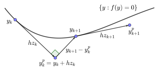
Figure 1: Illustration of the pseudo-arclength method: via a predictor-corrector scheme, for a given point $y_{k}$ such that $f(y_{k})=0$ the method computes $y_{k+1}$ such that $f(y_{k+1})=0$ and a consistently-oriented tangent direction $z_{k+1}$ at $y_{k+1}$.

As is evident from Step (1) of the pseudo-arclength algorithm given above, it is necessary to start the method with an initial point $y_{0}$ such that $f(y_{0})=0$. We can find such a point near the start of the bifurcation branch by using the local bifurcation theory for the model, which yields curves $c=c(\varepsilon)$ and $\phi=\phi(x,\varepsilon)$ that trace the bifurcation branch for $\varepsilon>0$ small. Indeed, for small $\varepsilon_{0}>0$ fixed, consider

$$y_{0}^{*}:=\left(c(\varepsilon_{0}),\phi(x_{1};\varepsilon_{0}),\phi(x_{2};\varepsilon_{0}),\ldots,\phi(x_{N};\varepsilon_{0})\right).$$ (2.11)

This $y_{0}^{*}$ does not necessarily solve $f(y_{0}^{*})=0$, but by virtue of $\varepsilon_{0}$ being small, $y_{0}^{*}$ should be close to the solution curve. Thus we may use $y_{0}^{*}$ as a good “initial guess” for a nonlinear system solver applied to finding $\left(\phi_{N,0}^{1},\phi_{N,0}^{2},\ldots,\phi_{N,0}^{N}\right)$ such that

$$f\left(c(\varepsilon_{0}),\phi_{N,0}^{1},\phi_{N,0}^{2},\ldots,\phi_{N,0}^{N}\right)=0.$$

We use this solution to form the initial point on the solution curve:

$$y_{0}:=\left(c(\varepsilon_{0}),\phi_{N,0}^{1},\phi_{N,0}^{2},\ldots,\phi_{N,0}^{N}\right).$$ (2.12)

Moreover, since the local bifurcation curve is parameterized by $\varepsilon$ for $\varepsilon>0$ small, we compute the tangent direction to the local bifurcation curve at $y_{0}^{*}$ by differentiating with respect to $\varepsilon$ at $\varepsilon_{0}$ and normalizing to unit length:

$$z_{0}^{*}:=\left(c^{\prime}(\varepsilon_{0}),\frac{\partial\phi}{\partial\varepsilon}(x_{1};\varepsilon_{0}),\frac{\partial\phi}{\partial\varepsilon}(x_{2};\varepsilon_{0}),\ldots,\frac{\partial\phi}{\partial\varepsilon}(x_{N};\varepsilon_{0})\right),\quad z_{0}:=\frac{z_{0}^{*}}{\lvert z_{0}^{*}\rvert},$$

Now, $z_{0}^{*}$ is not necessarily tangent to the solution curve, but since $\varepsilon_{0}>0$ is small, $z_{0}^{*}$ is very nearly tangent to the solution curve at $y_{0}$ as found above, and we take $z_{0}:=z_{0}^{*}/\lvert z_{0}^{*}\rvert$ as the initial tangent direction.

Remark 2.3.

In practice it typically does not matter that $z_{0}$ is not exactly tangent to the solution curve at $y_{0}$. For that matter, $y_{0}^{*}$ as defined in (2.11) can typically be used as the initial starting point without the preliminary application of the solver discussed above to find a $y_{0}$ as defined in (2.12). The accuracy of $y_{0}^{*}$ and $z_{0}^{*}$ affects the quality of the first predictor $y_{1}^{p}$, but for small $\varepsilon_{0}$ these initial inaccuracies are mitigated by the Newton solver in steps (2) and (3) of the method to obtain $y_{1}$ and $z_{1}$. Then, fortunately, all future iterations will have highly accurate starting points and tangent directions from which to form their predictors.

3 Numerical Results

In this section, we present our main numerical results for each of the bidirectional Whitham models (1.2), (1.4), and (1.6). Precisely, we implement the program outlined by the numerical bifurcation methods described in Section 2 to compute small and large amplitude traveling periodic profiles, and we produce the global bifurcation diagrams of periodic traveling waves with fixed period. Moreover, we study the stability of these waves to localized, i.e. integrable on $\mathbb{R}$, perturbations by using a Fourier-Floquet-Hill method [3] to numerically compute the spectrum of the associated linearized operators. We begin our analysis by demonstrating the relevant details of the computations for the model (1.2). Since the details for the models (1.4) and (1.6) are highly similar, only a summary of the relevant formulas will be provided for these other models.

3.1 Analysis of System (1.2)

We begin our analysis by considering the existence of periodic traveling waves to the bidirectional Whitham model (1.2):

$$\left\{\begin{array}[]{rcl}u_{t}&=&-\eta_{x}-uu_{x}\\ \eta_{t}&=&-\mathcal{K}u_{x}-(\eta u)_{x}.\end{array}\right.$$

Recall in the modeling of shallow water waves, $\eta$ represents the fluid height and $u$ is the trace of the velocity potential at the free surface. Transforming to traveling wave coordinates $x\mapsto x-ct$, such solutions are seen to be stationary, spatially periodic solutions $(u(x,t),\eta(x,t))=(\phi(x),\psi(x))$ of the evolutionary equation

$$\left\{\begin{array}[]{rcl}u_{t}&=&-\eta_{x}-uu_{x}+cu_{x}=:F(u,u_{x},\eta,\eta_{x};c)\\ \eta_{t}&=&-\mathcal{K}u_{x}-(\eta u)_{x}+c\eta_{x}=:G(u,u_{x},\eta,\eta_{x};c),\end{array}\right.$$ (3.1)

and hence the profiles $\phi,\psi$ satisfy the system

$$\left\{\begin{array}[]{rcl}0&=&-\psi^{\prime}-\phi\phi^{\prime}+c\phi^{\prime}\\ 0&=&-\mathcal{K}\phi^{\prime}-(\psi\phi)^{\prime}+c\psi^{\prime}.\end{array}\right.$$ (3.2)

Upon integrating (3.2) and setting constants of integration to zero, we can resolve $\psi$ in terms of $\phi$ in (3.2) to obtain

$$\psi =c\phi-\frac{1}{2}\phi^{2}$$

$$\mathcal{K}\phi =\frac{1}{2}\phi^{3}-\frac{3}{2}c\phi^{2}+c^{2}\phi=:g(c,\phi).$$ (3.3)

As explained in [6], one should not expect (3.3) to admit smooth solutions of arbitrary amplitude. Indeed, notice if $\phi$ is an $H^{1}$ solution of (3.3) then differentiating (3.3) yields

$$\mathcal{K}\phi^{\prime}=\left(\frac{3}{2}\phi^{2}-3c\phi+c^{2}\right)\phi^{\prime}\implies\phi^{\prime}=\frac{\mathcal{K}\phi^{\prime}}{\frac{3}{2}\phi^{2}-3c\phi+c^{2}}.$$ (3.4)

The operator $\mathcal{K}$ improves the smoothness of its operand by exactly one order, hence by (3.4) we have that $\phi^{\prime}$ is as smooth as $\phi$ so long as $\frac{3}{2}\phi^{2}-3c\phi+c^{2}\neq 0$, in which case a bootstrap argument demonstrates that $\phi$ is in fact $C^{\infty}$. When continuing from constant solutions, i.e. solutions with height zero, the breakdown of smoothness occurs when $\frac{3}{2}\phi^{2}-3c\phi+c^{2}=0$ or, more precisely, when the bifurcation branch intersects the curve $\phi=c\left(1-\frac{1}{\sqrt{3}}\right)$. Thus we expect (as is shown in [6]) that periodic solutions of (3.3) along the bifurcation branch with fixed period will have a maximum amplitude of

$$\max\phi(x)=\gamma:=c\left(1-\frac{1}{\sqrt{3}}\right).$$

See [6] for details of the above arguments.

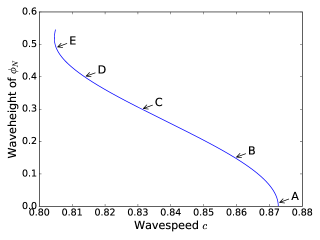
(a)

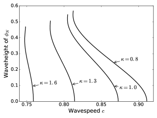
(b)

Figure 2: (a) A numerical approximation of the global bifurcation branch of $2\pi$-periodic ($\kappa=1$), even traveling solutions of (3.3) is displayed, with specific points A-E labeled for forthcoming computations: Point A at $c\approx 0.8726$, height $\approx 0.01$; Point B at $c\approx 0.8595$, height $\approx 0.15$; Point C at $c\approx 0.8312$, height $\approx 0.30$; Point D at $c\approx 0.8138$, height $\approx 0.40$; Point E at $c\approx 0.8051$, height $\approx 0.49$. (b) Bifurcation branches of $2\pi/\kappa$-periodic solutions of (3.3) for varying values of $\kappa$. Notice all these curves experience a turning point near the top of the branch.

3.1.1 Analysis of Waves Bifurcating from Zero

We begin by studying the bifurcation of $2\pi/\kappa$-periodic traveling wave solutions of (3.3) bifurcating from the trivial state $\phi=0$. To this end, using the profile equation (3.3) in combination with the following local bifurcation formulas (see [6, Proposition 5.1])

$$\phi(x;\varepsilon) :=\varepsilon\cos(\kappa x)+\frac{3c_{\kappa}\varepsilon^{2}}{4}\left(\frac{1}{c_{\kappa}^{2}-1}+\frac{\cos(2\kappa x)}{c_{\kappa}^{2}-c_{2\kappa}^{2}}\right)+O(\varepsilon^{3})$$ (3.5)

$$c(\varepsilon) :=c_{\kappa}+\frac{3\varepsilon^{2}}{8}\left[-\frac{1}{2c_{\kappa}}+3c_{\kappa}\left(\frac{1}{c_{\kappa}^{2}-1}+\frac{1}{2(c_{\kappa}^{2}-c_{2\kappa}^{2})}\right)\right],\quad c_{\ell}:=\sqrt{\frac{\tanh(\ell)}{\ell}},$$ (3.6)

we apply the pseudo-arclength method as discussed in Section 2.2 to compute approximations $\phi_{N}(x_{i})$ of the profile $\phi(x_{i})$ at the collocation points $x_{i}=\dfrac{(2i-1)\pi}{\kappa N}$, continuing while $\phi(0)\approx\phi_{N}(x_{1})<\gamma$. A global bifurcation plot of waveheight vs. wavespeed for various wavenumbers $\kappa$ is shown in Figure 2(b), where we define

$$\text{waveheight}:=\max_{x\in[0,\pi/\kappa]}\phi(x)-\min_{x\in[0,\pi/\kappa]}\phi(x)=\phi(0)-\phi(\pi/\kappa),$$

which is well-defined due to the monotonicity properties of even solutions along the global bifurcation branch as demonstrated in [6].

To illustrate the our numerical results for this model, we sample a selection of points along the global bifurcation diagram as described in Figure 2(a). As shown in Figure 3(a), the crest at the maximum of the smooth profiles along the global bifurcation branch becomes sharper as the waveheight increases, appearing to converge to a non-trivial profile with a singularity at the origin. The existence and qualitative properties of this highest singular wave has been studied analytically in [6], where it was shown the highest wave has a logarithmic cusp of order $\lvert x\ln\lvert x\rvert\rvert$ near the top of the bifurcation curve: see Figure 3(b). We refer the interested reader to [6] for details.

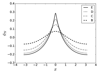
(a)

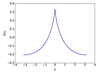
(b)

Figure 3: (a) Profiles corresponding to the sampled points on the branch of $2\pi$-periodic solutions of in Figure 2(a): Point B at $c\approx 0.8595$, height $\approx 0.15$; Point C at $c\approx 0.8312$, height $\approx 0.30$; Point D at $c\approx 0.8138$, height $\approx 0.40$; Point E at $c\approx 0.8051$, height $\approx 0.49$. (b) A nearly “highest” wave high up the bifurcation branch in Figure 2(a).

In addition to the existence of a highest singular wave, we also wish to understand the dynamical stability of the smooth periodic solutions constructed above. To this end, we wish to determine the spectrum of the linearization of (3.1) about such a smooth periodic traveling wave $\phi$. To linearize the traveling wave system (3.1) about the velocity profile $\phi$ described above and the corresponding height profile $\psi=c\phi-\dfrac{1}{2}\phi^{2}$, we write

$$\begin{array}[]{rcl}u(x,t)&=&\phi(x)+\varepsilon v(x,t)+\mathcal{O}(\varepsilon^{2})\\ \eta(x,t)&=&\psi(x)+\varepsilon w(x,t)+\mathcal{O}(\varepsilon^{2})\end{array}$$ (3.7)

where here, since we are interested in the stability to localized perturbations, we require that $v(\cdot,t),w(\cdot,t)\in L^{2}(\mathbb{R})$. for each time $t>0$ for which they are defined. Substituting these expansions into the first equation of (3.1) yields

$$\varepsilon v_{t} =(-\psi^{\prime}-\phi\phi^{\prime}+c\phi^{\prime})+\varepsilon\left[-\phi^{\prime}v+(c-\phi)v_{x}-w_{x}\right]+\mathcal{O}(\varepsilon^{2})$$

$$\varepsilon w_{t} =(-\mathcal{K}\phi^{\prime}-(\psi\phi)^{\prime}+c\psi^{\prime})+\varepsilon\left[-\psi^{\prime}v-\psi v_{x}-\mathcal{K}v_{x}-\psi^{\prime}w+(c-\phi)w\right]+\mathcal{O}(\varepsilon^{2})$$ (3.8)

as $\varepsilon\to 0$, where the $\mathcal{O}(1)$ terms vanish per the equilibrium system (3.2). Taking $\varepsilon\to 0$ above and decomposing the perturbations as $(v(x,t),w(x,t))=e^{\lambda t}(v(x),w(x))$ yields the spectral problem

$$\left\{\begin{aligned} \lambda v&=-\phi^{\prime}v+(c-\phi)v_{x}-w_{x}\\ \lambda w&=-\psi^{\prime}v-\psi v_{x}-\mathcal{K}v_{x}-\psi^{\prime}w+(c-\phi)w\\ &\qquad=:\mathcal{L}\left[\begin{array}[]{c}v\\ w\end{array}\right]\end{aligned}\right.$$ (3.9)

considered on $L^{2}(\mathbb{R})\times L^{2}(\mathbb{R})$.

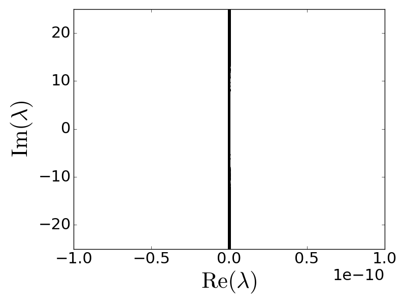
(a)

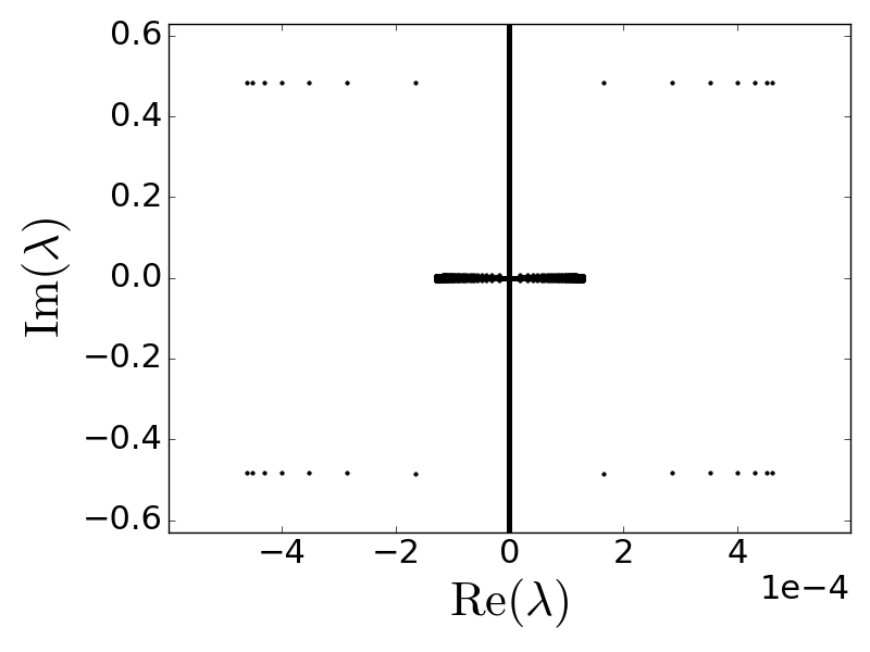
(b)

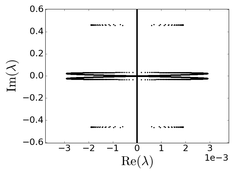
(c)

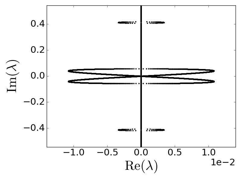
(d)

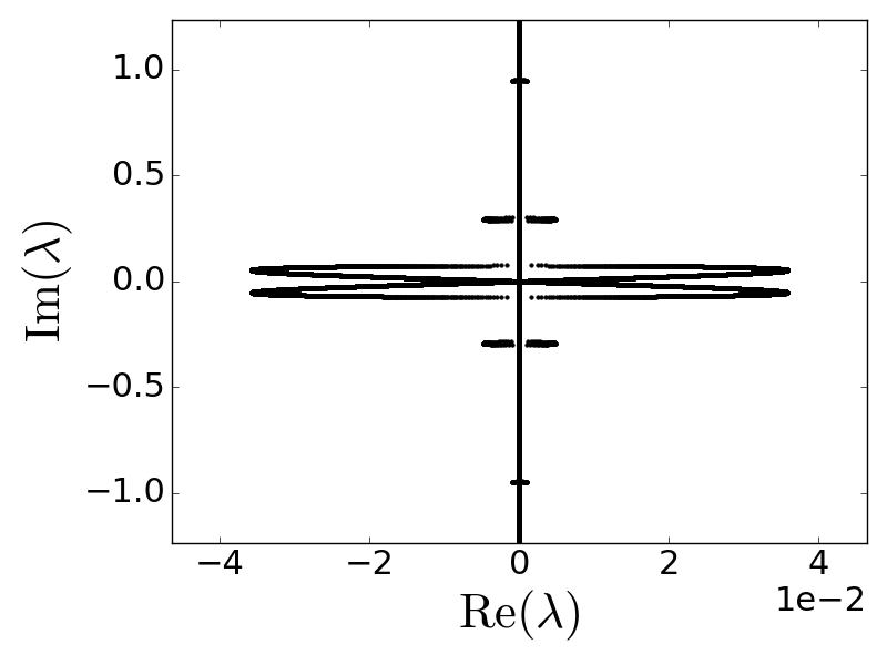
(e)

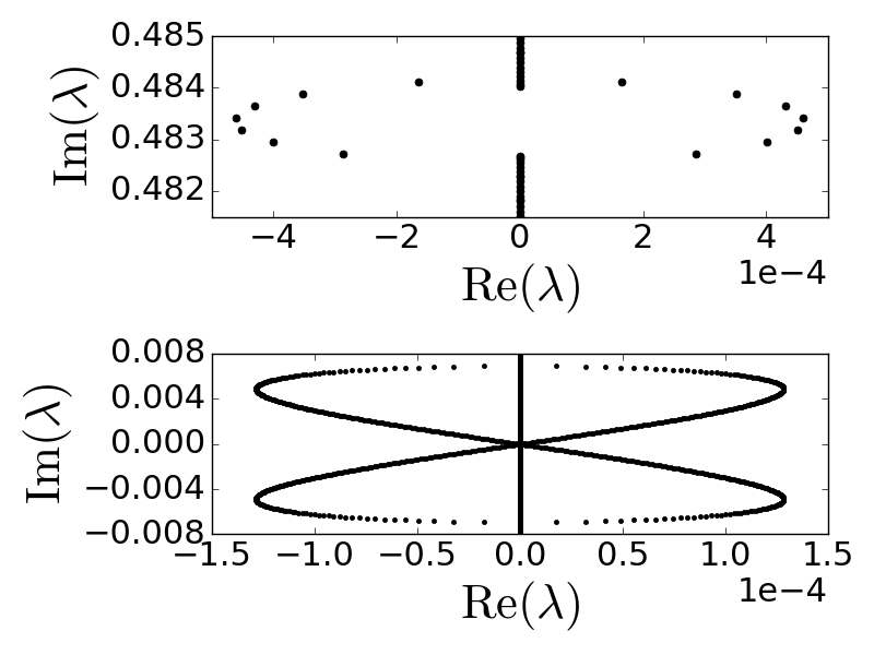
(f)

Figure 4: (a)-(e) Numerical approximations of the spectrum of $\mathcal{L}$ corresponding to the linearization of (1.2) about the profiles corresponding to the points A-E, respectively, along the bifurcation branch for $2\pi$-periodic solutions in Figure 2(a). (f) Zoom-in on the high-frequency instability (top) and the modulational instability (bottom) in the spectral plot (b).

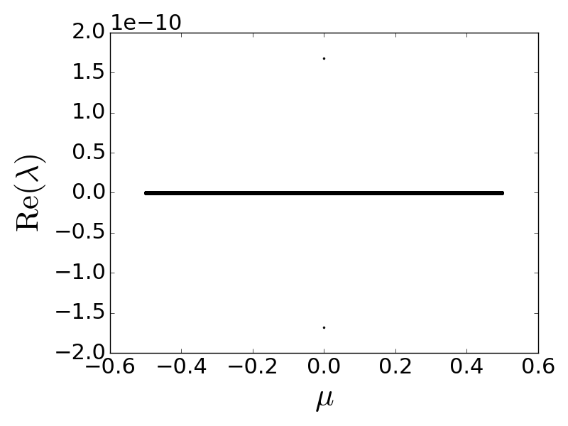
(a)

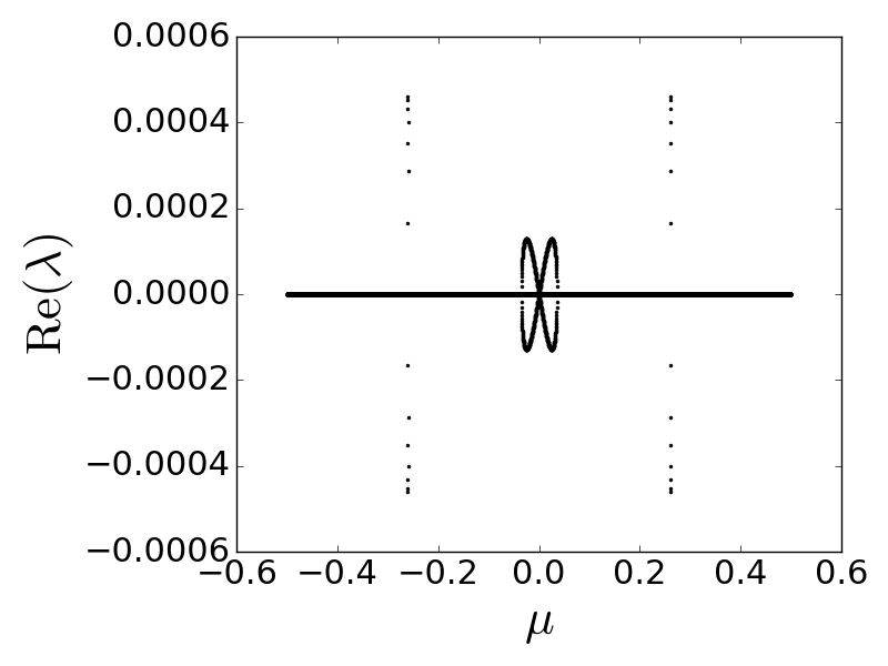
(b)

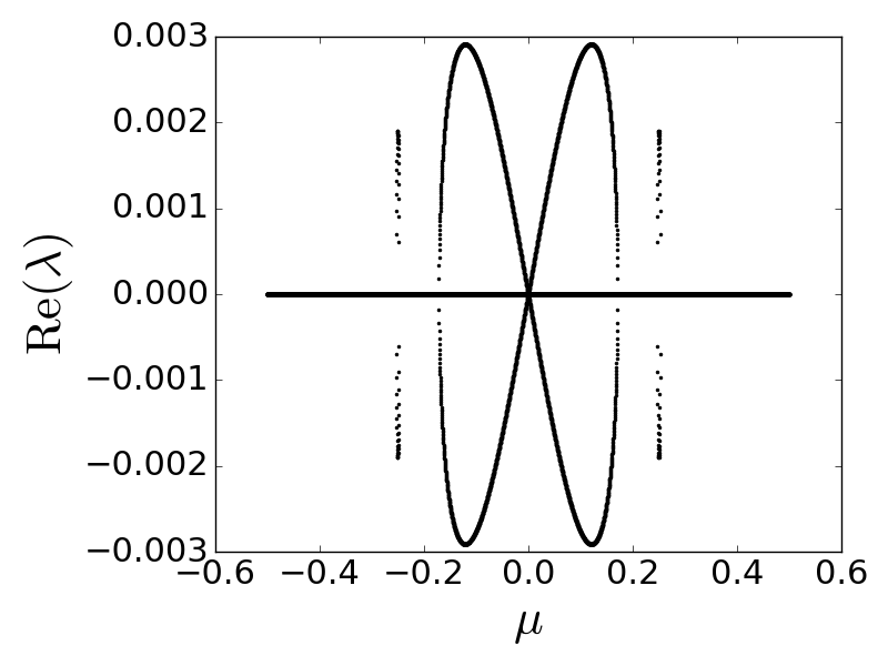
(c)

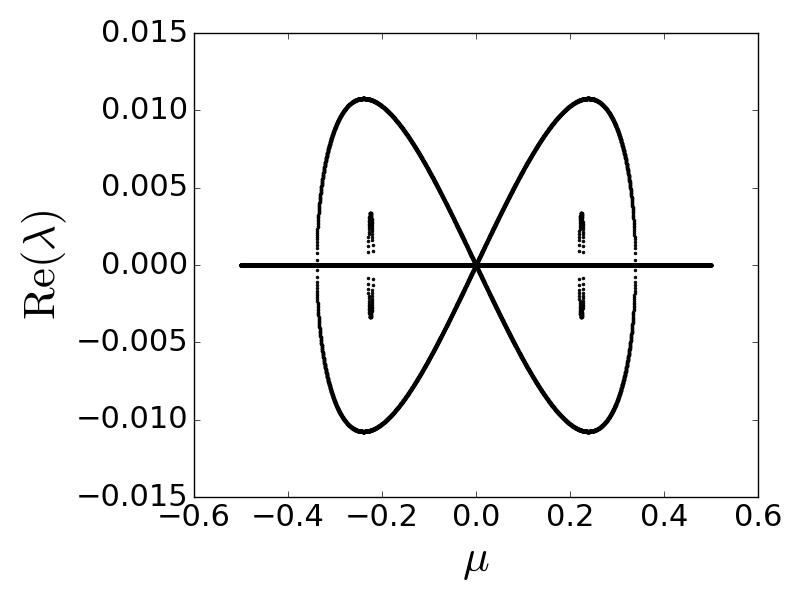
(d)

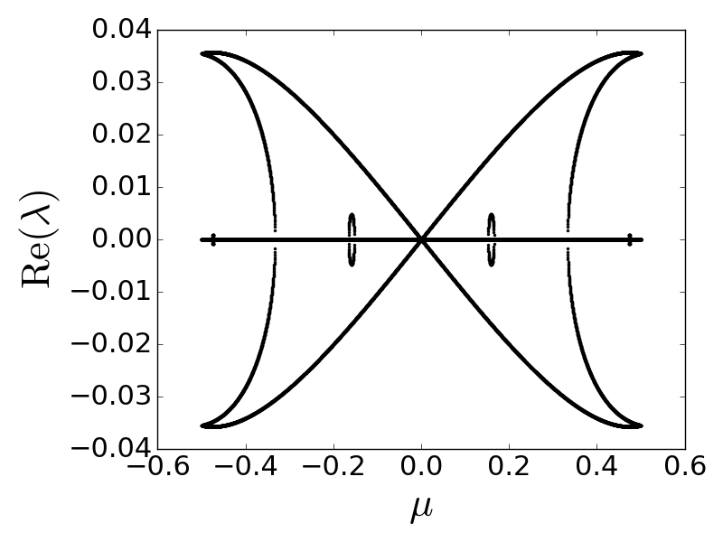
(e)

Figure 5: (a)-(e) Plots of the growth rates $\operatorname{Re}(\lambda)$ vs. $\mu$ for each of the spectral plots (a)-(e), respectively, in Figure 4.

By Floquet theory, we know the spectrum associated to $\mathcal{L}$ is purely essential, containing no isolated eigenvalues of finite multiplicity: see [20, 1]. Indeed, one can show that $\lambda$ belongs to the $L^{2}(\mathbb{R})$-spectrum of $\mathcal{L}$ if and only if there exists a so-called “Bloch parameter” $\mu\in[0,1)$ such that (3.9) has a bounded solution satisfying

$$(v,w)(x+2\pi/\kappa)=e^{i\kappa\mu}(v,w)(x)$$

for all $x\in\mathbb{R}$. It follows that the perturbations $(v,w)$ in (3.9) can be expanded in “Bloch” form as

$$\begin{array}[]{rcl}v(x)=\displaystyle\sum_{l\in\mathbb{Z}}\widehat{V}(l)e^{i\kappa(\mu+l)x},\quad w(x)=\displaystyle\sum_{l\in\mathbb{Z}}\widehat{W}(l)e^{i\kappa(\mu+l)x}.\end{array}$$ (3.10)

Substituting the expansions (3.10) for $v$ and $w$ into (3.9)(i), we obtain

$$\lambda\sum_{m\in\mathbb{Z}}\widehat{V}(m)e^{i\kappa mx} =\sum_{m\in\mathbb{Z}}\sum_{l\in\mathbb{Z}}\left[\left(ic\kappa(\mu+l)\delta_{m,l}-i\kappa(\mu+m)\widehat{\phi}(m-l)\right)\widehat{V}(l)-i\kappa(\mu+l)\widehat{W}(l)\right]e^{i\kappa mx},$$

where here $\widehat{\phi}(n)$ denotes the $n$th Fourier coefficient associated to the periodic profile $\phi$. It follows that each $m\in\mathbb{Z}$ we must have

$$\lambda\widehat{V}(m)=\sum_{l\in\mathbb{Z}}\left[\widehat{A}^{\mu}(m,l)\widehat{V}(l)+\widehat{B}^{\mu}(m,l)\widehat{W}(l)\right],$$ (3.11)

where

$$\widehat{A}^{\mu}(m,l) =ic\kappa(\mu+l)\delta_{m,l}-i\kappa(\mu+m)\widehat{\phi}(m-l)$$

$$\widehat{B}^{\mu}(m,l) =-i\kappa(\mu+l)\delta_{m,l}$$

and $\delta_{m,n}$ is the Kronecker delta. Similarly, substituting the expansions (3.10) into (3.9)(ii) yields, for each $m\in\mathbb{Z}$,

$$\lambda\widehat{W}(m)=\sum_{l\in\mathbb{Z}}\left[\widehat{C}^{\mu}(m,l)\widehat{V}(l)+\widehat{D}^{\mu}(m,l)\widehat{W}(l)\right],$$ (3.12)

where

$$\widehat{C}^{\mu}(m,l) =-i\kappa(\mu+m)\widehat{\psi}(m-l)-i\kappa(\mu+l)\widehat{\mathcal{K}}(\kappa(\mu+l))\delta_{m,l}$$

$$\widehat{D}^{\mu}(m,l) =ic\kappa(\mu+l)\delta_{m,l}-i\kappa(\mu+m)\widehat{\phi}(m-l).$$

Defining the bi-infinite matrices

$$\widehat{A}^{\mu}:=[\widehat{A}^{\mu}(m,l)]_{m,l\in\mathbb{Z}},\quad\widehat{B}^{\mu}:=[\widehat{B}^{\mu}(m,l)]_{m,l\in\mathbb{Z}},\quad\widehat{C}^{\mu}:=[\widehat{C}^{\mu}(m,l)]_{m,l\in\mathbb{Z}},\quad\widehat{D}^{\mu}:=[\widehat{D}^{\mu}(m,l)]_{m,l\in\mathbb{Z}}.$$

entry-wise for row-$m$ and column-$l$ with $m,l\in\mathbb{Z}$, the system (3.11)-(3.12) can be written in block bi-infinite matrix form as

$$\lambda\left[\begin{array}[]{c}\widetilde{V}\\ \hline\cr\widetilde{W}\end{array}\right]=\left[\begin{array}[]{c|c}\widehat{A}^{\mu}&\widehat{B}^{\mu}\\ \hline\cr\widehat{C}^{\mu}&\widehat{D}^{\mu}\end{array}\right]\left[\begin{array}[]{c}\widetilde{V}\\ \hline\cr\widetilde{W}\end{array}\right]=:\widehat{\mathcal{L}}^{\mu}\left[\begin{array}[]{c}\widetilde{V}\\ \hline\cr\widetilde{W}\end{array}\right],$$ (3.13)

where $\widetilde{V},\widetilde{W}$ denote the bi-infinite arrays

$$\left\{\begin{aligned} \widetilde{V}&:=\begin{bmatrix}\ldots&\widetilde{V}(-2)&\widetilde{V}(-1)&\widetilde{V}(0)&\widetilde{V}(1)&\widetilde{V}(2)&\ldots\end{bmatrix}^{T}\\ \widetilde{W}&:=\begin{bmatrix}\ldots&\widetilde{W}(-2)&\widetilde{W}(-1)&\widetilde{W}(0)&\widetilde{W}(1)&\widetilde{W}(2)&\ldots\end{bmatrix}^{T}.\end{aligned}\right.$$

For each $\mu$, the spectrum of $\widehat{\mathcal{L}}^{\mu}$ consists of countably many discrete eigenvalues with finite multiplicity and, furthermore, by the above considerations we have the spectral decomposition

$$\sigma_{L^{2}(\mathbb{R})}(\mathcal{L})=\bigcup_{\mu\in[0,1)}\sigma(\widehat{\mathcal{L}}^{\mu}).$$

We numerically approximate the spectrum of the bi-infinite matrix $\widehat{\mathcal{L}}^{\mu}$ by taking a sequence of $\mu$ in a finite discretization of $[0,1)$, truncating each block of $\widehat{\mathcal{L}}^{\mu}$ in (3.13) to finite dimension, and computing the eigenvalues of the truncated matrix using a standard matrix eigenvalue solver. See Appendix A for further discussion. See Figure 4 for plots of the spectrum at the sampled points on the bifurcation diagram of $2\pi$-periodic solutions in Figure 2(a), as well as Figure 5 for plots of the growth rate $\operatorname{Re}(\lambda)$ vs. the Bloch parameter $\mu$. It is known that the full Euler equations exhibit high-frequency instabilities (visually characterized by “bubbles” of spectrum emanating from the imaginary axis from points away from the origin) in small-amplitude periodic traveling waves; however, we discover that while this model demonstrates both high-frequency and modulational instabilities for waves of sufficiently high amplitude, a high-frequency instability is numerically undetectable for small amplitude waves: see Figure 4(a) and Figure 5(a) below. Whether such instabilities are actually nonexistent or simply not detected for small amplitude waves in our numerics is unclear.

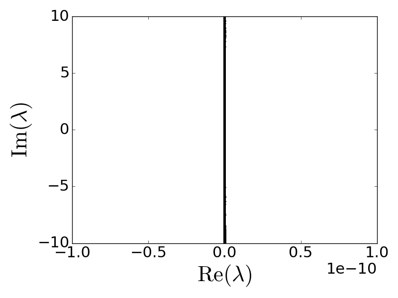
(a)

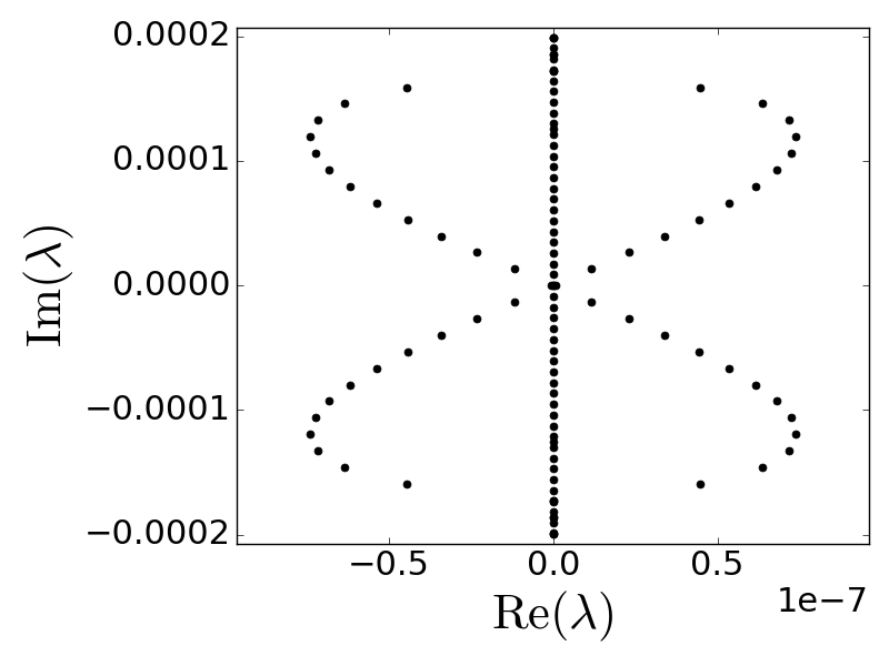
(b)

Figure 6: Evidence of the Benjamin-Feir instability in (1.2) for waveheight $0.01766$. In(a) we have $\kappa=1.005$ while in (b) we have $\kappa=1.008$.

Solutions of different wavelength can be generated by varying the value of $\kappa$, as shown in the plot of the bifurcation diagrams for various $\kappa$ in Figure 2(b). In [11], an analysis of asymptotically small amplitude waves shows that there exists a critical value $\kappa_{c}$ such that all waves are modulationally unstable for all $\kappa>\kappa_{c}$ where $\kappa_{c}\approx 1.008$. Inspired by this analysis, we performed numerical experiments varying the value of $\kappa$ for small, but fixed, waveheights, finding very good agreement with the results in [11]. Figure 6(a) demonstrates that waves with waveheight $0.01766$ and corresponding to $\kappa=1.005$ are modulationally stable, while for $\kappa=1.008$ a modulational instability appears for waves of the same height: see Figure 6(b).

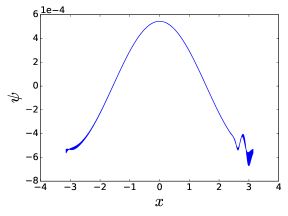
(a)

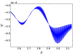
(b)

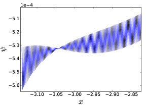
(c)

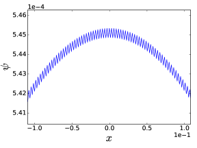
(d)

Figure 7: Numerical evidence of ill-posedness of (1.2) for initial data $\eta(x,0)=\psi(x)$ having negative infimum. (a) The result of a short time evolution of a $2\pi$-periodic wave ($\kappa=1$) with small waveheight $\max\psi-\min\psi\approx 0.00109$, $c\approx 0.872693$. We zoom in near the rightmost and leftmost of the waves in (b) an (c), respectively. In (d) we observe that oscillations also are forming near the positive maxima, although the oscillations there are not as pronounced as near the minima.

3.1.2 Time Evolution and Ill-Posedness

The numerical findings in the previous section are restricted to waves bifurcating from the zero constant state in the bidirectional Whitham model (1.2). This is largely motivated by the fact that the authors have recently analytically studied the structure of the global bifurcation branch in [6]. In an effort to understand the nonlinear dynamics about the numerically computed profiles in Figure 2(a), we use a sixth-order pseudospectral operator splitting method [25] to evolve (3.1) with the numerical solutions as initial data, with the expectation that the initial profile translates as a traveling wave with corresponding wavespeed $c$, mapping onto itself after an integral number of temporal periods $T=\frac{2\pi}{\kappa c}$. Interestingly, however, such time evolution attempts failed, resulting in wild oscillations after a short amount of time, e.g. 35.4% of a temporal period for a $2\pi$-periodic wave of small waveheight $\max\psi-\min\psi\approx 0.00109$ and wavespeed $c\approx 0.872693$. See Figure 7. This seems to suggest that either the solutions computed in Figure 2(a) are in fact not traveling wave solutions of (1.2), or that the local evolution in the PDE (1.2) about such waves is ill-posed.

In this direction, we note that it has recently been reported in [8, Theorem 1] that (1.2) is locally well-posed for all initial data $\eta(x,0)=\psi(x)$, $u(x,0)=\phi(x)$ with $\inf_{x\in[0,2\pi)}\psi(x)>0$. As the height profiles about the waves along the bifurcation curves constructed above all have a strictly negative infimum, it follows that the local well-posedness result in [8] does not apply to the waves constructed in the previous section and hence, by extension, also not to the waves constructed in [6]. The time evolution results reported in Figure 7 strongly indicate that the positivity assumption on the height profile $\eta$ in [8] is sharp and cannot be removed in general.

In contrast, waves of (1.2) having strictly positive profile that are constructed by bifurcating from a positive constant state exhibit local well-posedness in time. See Figure 10 and the surrounding discussion. See Appendix B.2 for further details about the time evolution.

3.1.3 Analysis of Waves with Positive Height Profile

Given the well-posedness result discussed above and the apparent failure of the waves considered in Section 3.1.1 to have well-posed local dynamics, it is natural to attempt to construct wavetrain solutions of (1.2) for which the local evolution is well-posed. With the result of [8] in mind, we seek to construct solutions of (3.1) that have strictly positive height profiles $\eta(x)$ by bifurcating from a positive constant state. As discussed in [6], the curves of trivial solutions for (3.1) are given by

$$c\mapsto 0,\quad c\mapsto\Gamma_{\pm}(c):=\frac{3c\pm\sqrt{8+c^{2}}}{2},$$

and the waves studied in Section 3.1 above bifurcate from the zero-amplitude state, with the height profiles $\eta(x)$ all having strictly negative infima. Since $\Gamma_{-}(c)>0$ for all $c>1$, this motivates an attempt to construct waves that bifurcate from the $\Gamma_{-}$ curve, which (at least for small waveheight) are guaranteed to fall into the regime of well-posedness: see Figure 8 below.

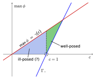
(a)

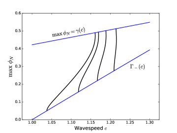
(b)

Figure 8: (a) Bifurcation diagram of (3.3). Waves bifurcating from the zero state are likely ill-posed, while waves bifurcating from a non-zero constant state (curve $\Gamma_{-}$) are well-posed. (b) Numerical approximations of the bifurcation branches of even, one-sided monotone, $2\pi/\kappa$ periodic solutions of (3.3). From left to right, $\kappa=0.5,1.0,1.3,1.6$.

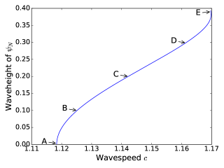
(a)

(b)

Figure 9: Positive $2\pi$-periodic equilibrium profiles $\eta(x,t)=\psi(x)$ bifurcating from constant positive state. In (a), we show the global bifurcation branch with points A-E labeled for forthcoming computations: Point A at $c\approx 1.1184$, height $\approx 0.003$; Point B at $c\approx 1.1252$, height $\approx 0.15$; Point C at $c\approx 0.8312$, height $\approx 0.30$; Point D at $c\approx 0.8138$, height $\approx 0.40$; point E at $c\approx 0.8051$, height $\approx 0.49$. In (b), we show the height profiles $\psi$ associated to the waves A-E of increasing waveheight along the branch in (a).

To this end, observe that non-zero constant profiles $\phi$ of (3.3) satisfy

$$Q(\phi;c):=c^{2}-1-\frac{3}{2}c\phi+\frac{1}{2}\phi^{2}=0.$$ (3.14)

Let $(\phi_{*},c_{*})$ be a solution of (3.14) for $c_{*}>1$. In order for non-trivial, real-valued, even, periodic solutions to branch from the constant state at $c_{*}$, the kernel of the Frechet derivative $\delta_{\phi}Q(\phi_{*};c_{*})$ must be non-trivial. If $v\in\ker(\delta_{\phi}Q(\phi_{*};c_{*}))$ with $v(x)=\sum_{n=0}^{\infty}\widehat{v}(n)\cos(n\kappa x)$, then

$$0=\delta_{\phi}Q(\phi_{*};c_{*})v=\left(\mathcal{K}-c^{2}+3c\phi_{*}-\frac{3}{2}\phi_{*}^{2}\right)v.$$

Taking the Fourier transform yields

$$0=\left(\widehat{\mathcal{K}}(\kappa n)-c^{2}+3c\phi_{*}-\frac{3}{2}\phi_{*}^{2}\right)\widehat{v}(n),\quad n\in\mathbb{N}_{0},$$

and we see that if

$$\widehat{\mathcal{K}}(\kappa n_{0})-c^{2}+3c\phi_{*}-\frac{3}{2}\phi_{*}^{2}=0$$ (3.15)

for fixed $n_{0}\in\mathbb{N}_{0}$, then

$$\operatorname{span}\{\cos(\kappa n_{0}x)\}=\ker(\delta_{\phi}Q(\phi_{*},c_{*})).$$

Combining and (3.15) yields a system of necessary conditions for a non-trivial branch of $2\pi/(\kappa n_{0})$-periodic traveling wave solutions of (1.2) to appear:

$$\left\{\begin{array}[]{rcl}\displaystyle c_{*}^{2}-1-\frac{3}{2}c_{*}\phi_{*}+\frac{1}{2}\phi_{*}^{2}&=&0\vspace{0.5em}\\ \displaystyle\widehat{\mathcal{K}}(\kappa n_{0})-c_{*}^{2}+3c_{*}\phi_{*}-\frac{3}{2}\phi_{*}^{2}&=&0.\end{array}\right.$$ (3.16)

For positive wavespeed, this system has a unique solution $(c_{*}(n_{0}),\phi_{*}(n_{0}))$ for each $n_{0}\in\mathbb{N}_{0}$. In the case of $n_{0}=1$, corresponding to $2\pi$-periodic solutions of (3.3), we find

$$c_{*}\approx 1.11834,\quad\phi_{*}\approx 0.15677.$$

By standard Lyapunov-Schmidt arguments, it can be shown that a local bifurcation of $2\pi$-periodic wavetrains of asymptotically small waveheight occurs at $(\phi_{*},c_{*})$. In particular, one finds the following local bifurcation formulas:

$$\phi(x;a) :=\phi_{*}+a\cos(\kappa n_{0}x)+O(a^{2})$$

$$c(a) :=c_{*}+\frac{3-4q}{24\phi_{*}-16c_{*}}a^{2}+O(a^{3}),\quad q:=\frac{3}{4}\left[\frac{\phi_{*}-c_{*}}{\widehat{\mathcal{K}}(2\kappa n_{0})-c_{*}^{2}+3c_{*}\phi_{*}-\frac{3}{2}\phi_{*}^{2}}\right].$$

Using the methods of Section 2 to approximate the wave profiles, we obtain a branch of solutions, depicted in Figure 9 as waveheight vs. wavespeed, with all the height profiles $\psi$ possessing a strictly positive infimum and an increasingly sharp crest for large waveheights. In particular, we note that the time evolution about these waves indeed appears to be well-posed. In fact, a time evolution of a $2\pi$-periodic solution of (1.2) with wavespeed $c\approx 1.1698$ and $\max\psi-\min\psi\approx 0.387$ over 15 temporal periods $15T=15\cdot 2\pi/c$ closely mapped the initial data onto itself, with residual

$$\|\eta(\cdot,15T)-\psi\|_{L^{2}}\approx 3.5\times 10^{-6}.$$

See Figure 10. This demonstrates that these computed profiles with positive minimum indeed form traveling wave solutions of (1.2) that exhibit locally well-posed time evolution.

Concerning the stability of these $2\pi$-periodic positive height waves, we find that they behave similarly to ill-posed waves discussed in the previous section, with waves of sufficiently large height demonstrating modulational and high-frequency instabilities: see Figure 11. In fact, Figure 11(a) suggests that $2\pi$-periodic waves of small amplitude exhibit modulational instability.

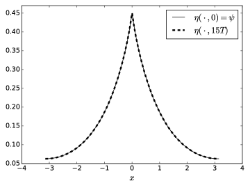
Figure 10: A time evolution of (1.2) using a positive equilibrium profile as initial data appears stationary after $15$ temporal periods, mapping closely onto itself.

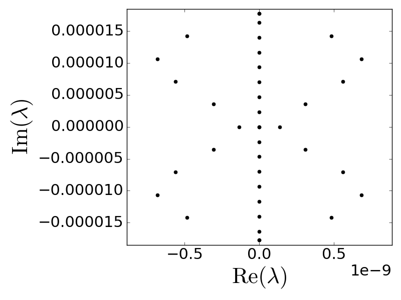
(a)

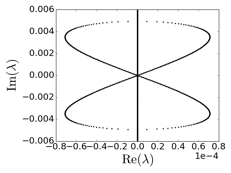
(b)

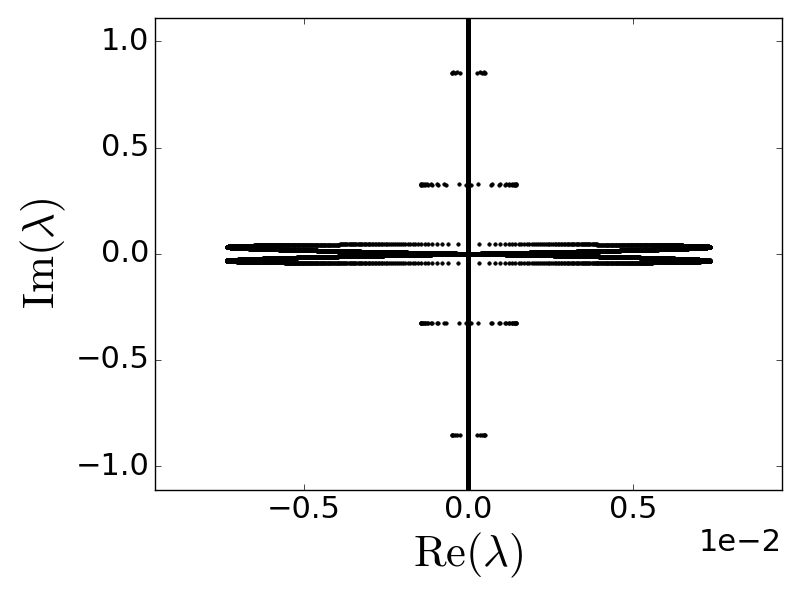
(c)

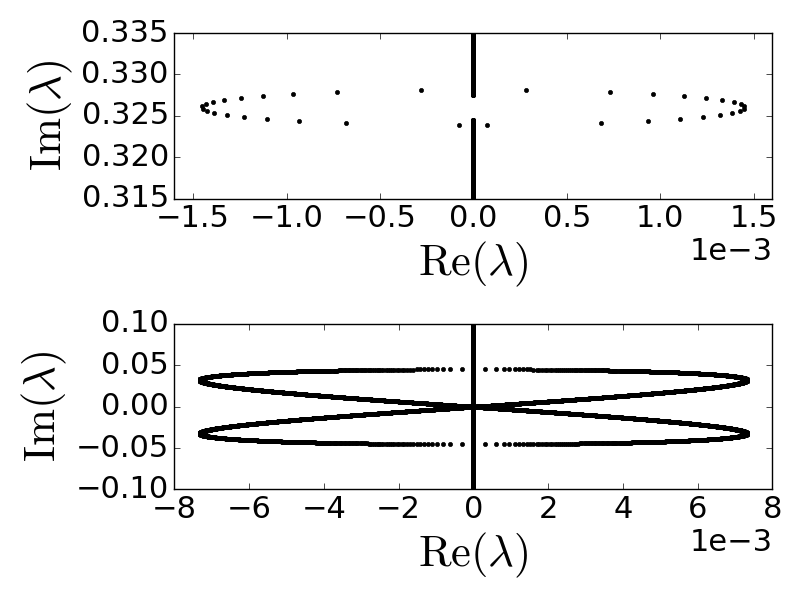
(d)

Figure 11: Spectral plots for $2\pi$-periodic positive waves for (1.2) at points A (a), B (b), and D (c) along the bifurcation branch of $2\pi$-periodic solutions in Figure 9. (d) Zoom-in on the high-frequency instability (top) and the modulational instability (bottom) in the spectral plot (c).

3.2 Analysis of System (1.4)

We now turn our attention to the bidirectional Whitham model (1.4):

$$\left\{\begin{array}[]{rcl}u_{t}&=&-\mathcal{K}\eta_{x}-uu_{x}\\ \eta_{t}&=&-u_{x}-(\eta u)_{x}.\end{array}\right.$$

In particular, we are interested in performing an analogous study for (1.4) that was performed for the model (1.2) in Section 3.1 above. Below, we compute global bifurcation diagrams, including large amplitude solutions, and analyze the spectrum of the linearization of (1.4) about these solutions.

As mentioned in the introduction, this model was proposed and analyzed in [11], which examines the local bifurcation and spectral stability of asymptotically small amplitude periodic traveling waves, finding that this model exhibits the Benjamin-Feir instability. Precisely, they prove the existence of a critical wave number $\kappa_{c}\approx 1.610$ such that asymptotically small-amplitude wavetrains of period $2\pi/\kappa$ are modulationally when $\kappa>\kappa_{c}$ (“super-critical”), while they are spectrally stable for $0<\kappa<\kappa_{c}$ (“subcritical”). Below, we numerically confirm this result for small amplitude waves, and also demonstrate that large amplitude waves are spectrally unstable in both the sub-critical and super-critical regimes. See Figure 14 for spectrum plots in the super-critical case and Figure 15 for spectrum plots the sub-critical case. Furthermore, from our experiments we make a conjecture regarding the nonexistence of a singular wave of greatest height.

To generate profiles, we follow the program of the numerical methods described in Section 2. First, we transform (1.4) to traveling wave coordinates:

$$\left\{\begin{array}[]{rcl}u_{t}&=&cu_{x}-\mathcal{K}\eta_{x}-uu_{x}=:F(u,u_{x},\eta,\eta_{x};c)\\ \eta_{t}&=&c\eta_{x}-u_{x}-(\eta u)_{x}=:G(u,u_{x},\eta,\eta_{x};c).\end{array}\right.$$

An equilibrium solution $(u,\eta)(x,t)=(\phi,\psi)(x)$ of the above traveling wave system satisfies

$$\left\{\begin{array}[]{rcl}-c\phi^{\prime}+\mathcal{K}\psi^{\prime}+\phi\phi^{\prime}&=&0\\ -c\psi^{\prime}+\phi^{\prime}+(\psi\phi)^{\prime}&=&0\end{array}\right.$$

which, upon integrating and setting integration constants to zero, yields

$$\left\{\begin{array}[]{rcl}-c\phi+\mathcal{K}\psi+\frac{1}{2}\phi^{2}&=&0\\ -c\psi+\phi+\psi\phi&=&0.\end{array}\right.$$

Then resolving $\phi$ in terms of $\psi$ yields the scalar profile equation

$$\mathcal{K}\psi=\frac{c^{2}\psi}{1+\psi}-\frac{c^{2}\psi^{2}}{2(1+\psi)^{2}}=:g(c,\psi).$$ (3.17)

Using the methods in Section 2.1, we numerically compute the bifurcation branch and periodic profiles with various waveheights with super-critical $\kappa=1.611$: see Figure 12(a)-(c). Further, in Figure 12(d) we compute bifurcation branches of $2\pi/\kappa$-periodic profiles for various $\kappa$.

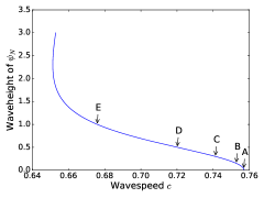
(a)

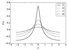
(b)

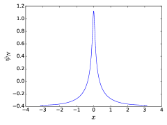
(c)

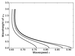
(d)

Figure 12: Bifurcation branches of (3.17) for super-critical $\kappa=1.611>\kappa_{c}$. (a) Locations on the bifurcation branch of periodic solutions corresponding to super-critical $\kappa=1.611$ of (3.17) that are sampled for profile and spectral plots: Point A at $c\approx 0.7569$, height $\approx 0.03$; Point B at $c\approx 7528$, height $\approx 0.15$; Point C at $c\approx 0.7412$, height $\approx 0.30$; Point D at $c\approx 0.7201$, height $\approx 0.50$; Point E at $c\approx 0.6759$, height $\approx 1.00$. (b) Profiles corresponding to the points along the bifurcation branch labeled in (a). (c) A super-critical wave ($\kappa=1.611$) of large waveheight; $c\approx 0.6745$, $\text{waveheight}\approx 1.500$. The crest of the wave is still smooth despite the large waveheight. (d) Numerical approximations of the $2\pi/\kappa$ periodic solutions of (3.17) with wavespeed $c$. From left to right, $\kappa=1.6,1.3,1,0.8$.

In contrast to the model (1.2) analyzed in Section 3.1 above, we conjecture that the bifurcation branches associated with (1.4) will not possess peaked/cusped waves of maximum height. In fact, we believe the profiles along the global bifurcation branches will be smooth for arbitrarily large waveheight. To understand this, observe that differentiating the profile equation (3.17) and rearranging yields

$$\psi^{\prime}=\frac{c^{2}}{(1+\psi)^{3}}\mathcal{K}\psi^{\prime}.$$

Since $\mathcal{K}\psi^{\prime}$ has the same regularity as $\psi$, we have that $\psi^{\prime}$ is smooth so long as the wave speed $c$ remains bounded away from zero and the profiles $\psi$ remain bounded away from $\psi=-1$ along the bifurcation branch. From Figure 12, it seems plausible that both of these conditions hold uniformly along the bifurcation branch, indicating that the bifurcation branch does not terminate in a highest wave. See Figure 12(d) for a periodic profile of large waveheight having a visibly smooth crest. We leave the analytical verification of this conjecture as an interesting open problem.

Remark 3.1.

Since this model is conjectured to not possess peaked/cusped waves of maximum height, the waveheight vs. wavespeed plots in Figures 12(a), (d) were stopped at height $3$. As seen in Figure 12(a), a turning point occurs near waveheight $3$, after which the wavespeed increases as the waveheight increases. Numerically, a second turning point is also observed for waves of larger height, but we believe that this second turning point is only due to truncation, at its location varies considerably as larger numbers of Fourier modes $N$ are used. See Figure 13.

Figure 13: Secondary turning points in the bifurcation diagrams for system (1.4) are present at large waveheight, but this is believed to be purely due to truncation since its location increases as the number of Fourier modes $N\in\{64,128,256,512\}$ increases.

To study the dynamical stability of the periodic wavetrains computed in Figure 12, we use the general methods of Appendix A. In particular, we build truncated bi-infinite matrices whose eigenvalues approximate the spectrum of the linearization:

$$\widehat{A}^{\mu}(m,l) =ic\kappa(\mu+l)\delta_{m,l}-i\kappa(\mu+m)\widehat{\phi}(m-l)$$

$$\widehat{B}^{\mu}(m,l) =-i\kappa(\mu+l)\widehat{\mathcal{K}}(\kappa(\mu+l))\delta_{m,l}$$

$$\widehat{C}^{\mu}(m,l) =-i\kappa(\mu+l)\delta_{m,l}-i\kappa(\mu+m)\widehat{\psi}(m-l)$$

$$\widehat{D}^{\mu}(m,l) =ic\kappa(\mu+l)\delta_{m,l}-i\kappa(\mu+m)\widehat{\phi}(m-l).$$

Plots of the spectrum at the sampled points along the bifurcation branch in Figure 12(a) are shown in Figure 14. In particular, Figure 14(a) demonstrates a modulational instability for a small waveheight, while the other plots for larger waveheights show both a modulational instability and a high-frequency instability. Moreover, plots of the growth rate $\operatorname{Re}(\lambda)$ vs. $\mu$ for the these spectra are shown in Figure 16. Moreover, the spectral stability of small-amplitude sub-critical solutions is shown in Figure 15(a), as predicted by analytical theory in [11]. However, even for $\kappa$ in the sub-critical regime, waves of sufficiently large waveheight develop both modulational and high-frequency instabilities (see Figure 15(b)) while small amplitude waves are spectrally stable. Moreover, waves are stable with respect to co-periodic perturbations.

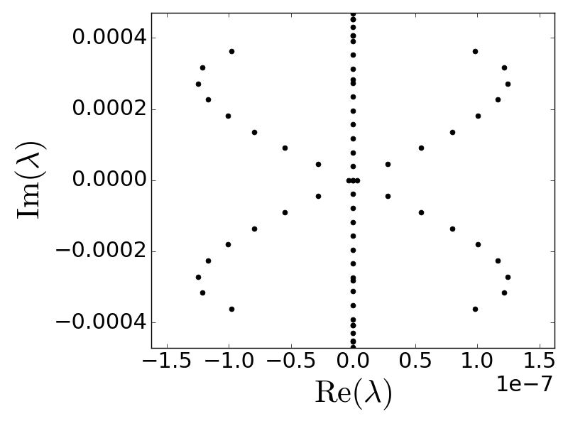
(a)

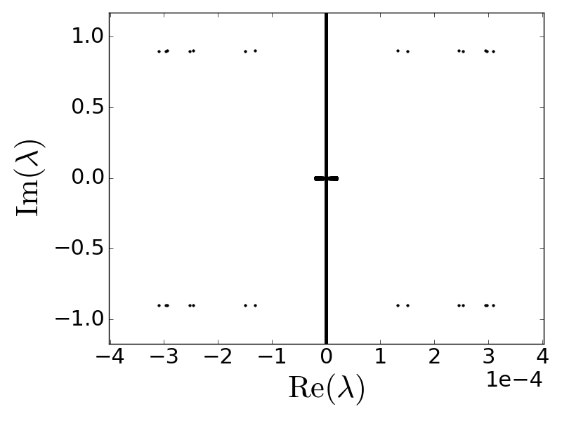
(b)

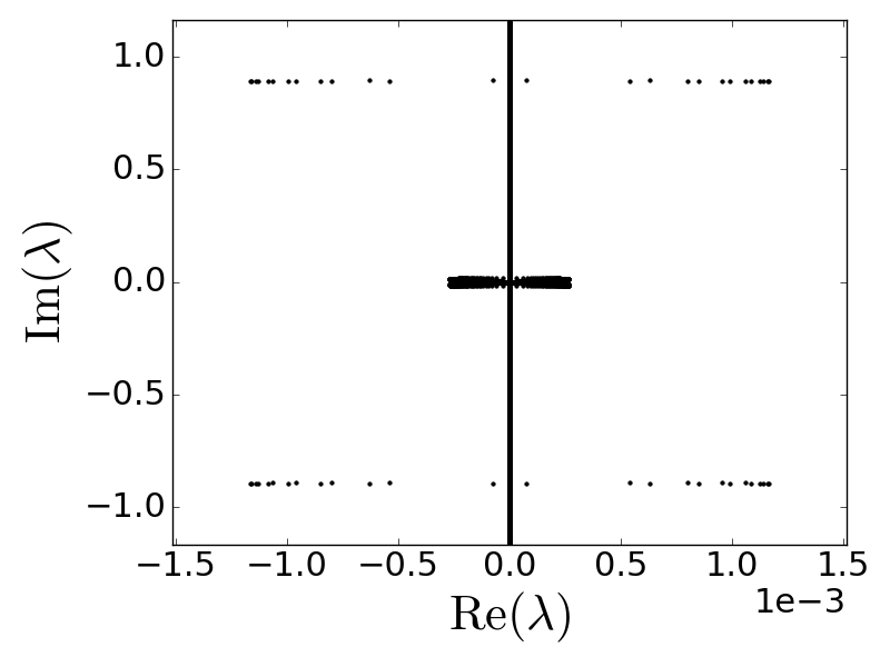
(c)

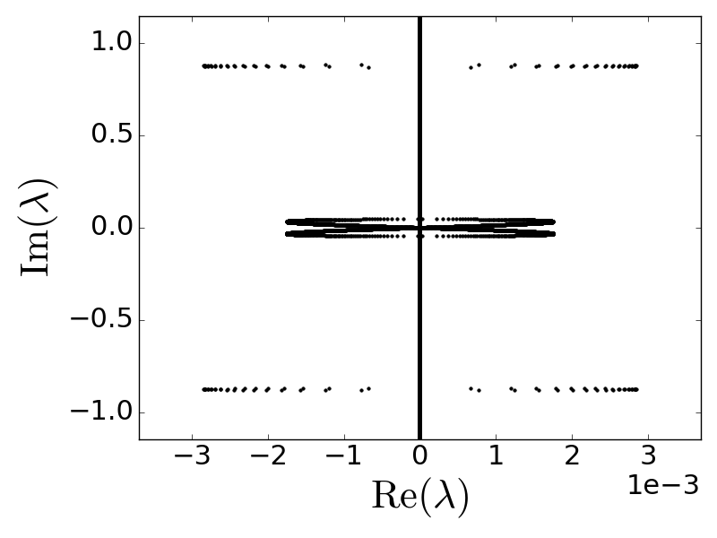
(d)

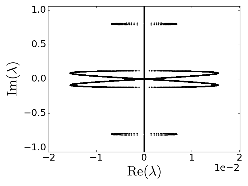
(e)

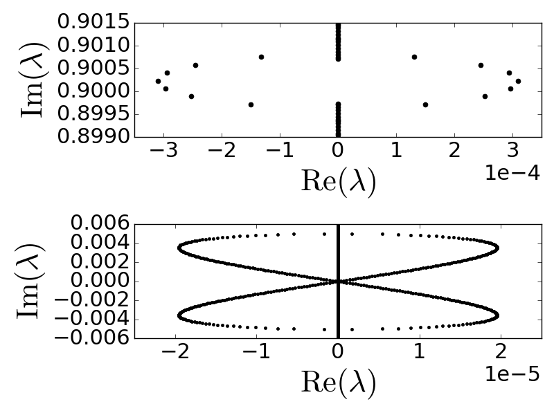
(f)

Figure 14: (a)-(e) Spectral plots for $2\pi/\kappa$-periodic waves A-E selected along the bifurcation branch in Figure 12(a) with super-critical $\kappa=1.611$. (f) Zoom-in on the high-frequency instability (top) and modulational instability (bottom) for the spectrum in (b).

(a)

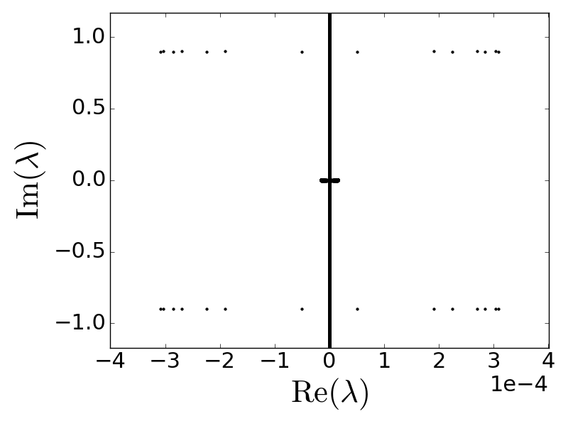
(b)

Figure 15: Spectral plots for small $2\pi/\kappa$-periodic solutions of (3.17) with sub-critical $\kappa=1.609<\kappa_{c}$). In (a), the waveheight of the underlying wave $\psi$ is $0.03$, while in (b) it is $0.15$.

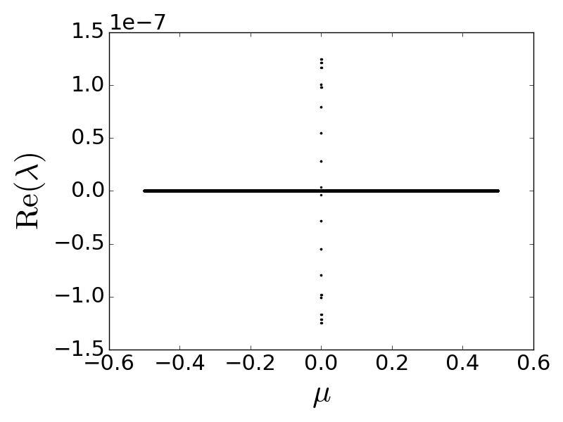
(a)

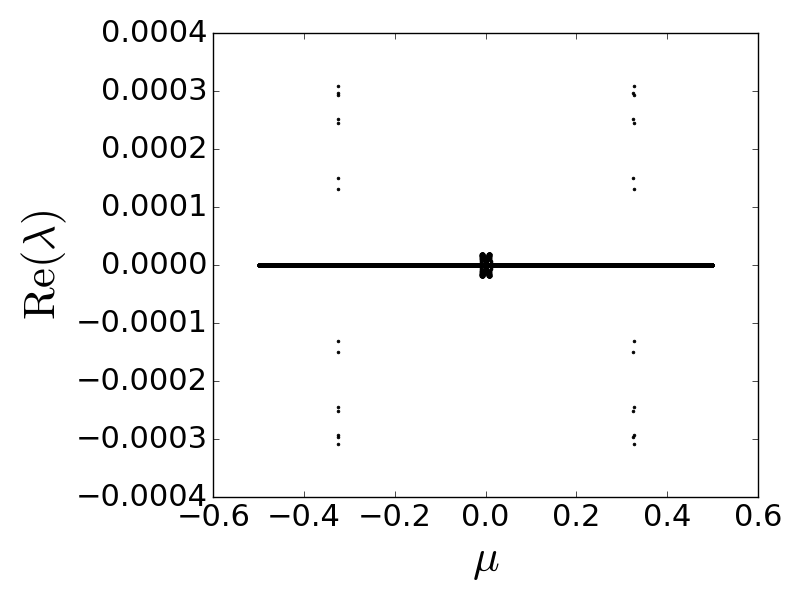
(b)

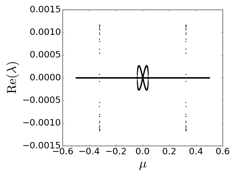
(c)

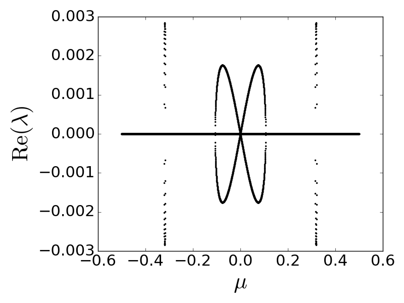
(d)

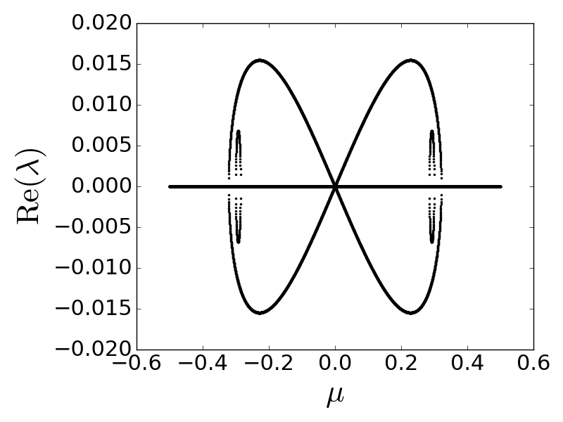
(e)

Figure 16: (a)-(e) $\operatorname{Re}(\lambda)$ vs. $\mu$ for each of the spectral plots (a)-(e), respectively, for the super-critical $\kappa$ in Figure 14.

3.3 Boussinesq-Whitham

Finally, we now turn our attention to the scalar Boussinesq-Whitham model (1.5) proposed in [5, Section 5]:

$$u_{tt}=\partial_{x}^{2}(u^{2}+\mathcal{K}u).$$

Since [5] does not provide details for the local bifurcation theory of this model, we sketch the Lyapunov-Schmidt reduction here. Writing the second order equation (1.5) as a first order system, we have

$$\left\{\begin{array}[]{rcl}u_{t}&=&\eta\\ \eta_{t}&=&\partial_{x}^{2}(u^{2}+\mathcal{K}u),\end{array}\right.$$

and changing to traveling wave coordinates yields

$$\left\{\begin{array}[]{rcl}u_{t}&=&\eta+cu_{x}=:F(u,u_{x},\eta,\eta_{x};c)\\ \eta_{t}&=&c\eta_{x}+\partial_{x}^{2}(u^{2}+\mathcal{K}u):=G(u,u_{x},\eta,\eta_{x};c).\end{array}\right.$$

Equilibrium solutions $(u,\eta)=(\phi,\psi)$ of this system satisfy

$$\left\{\begin{array}[]{rcl}-c\phi^{\prime}&=&\psi\\ -c\psi^{\prime}&=&(\phi^{2}+\mathcal{K}\phi)^{\prime\prime},\end{array}\right.$$ (3.18)

in which we can resolve $\psi$ in terms of $\phi$ by integrating the second equation, setting the resulting constant of integration to zero, yielding the relation

$$-c\psi=(\phi^{2}+\mathcal{K}\phi)^{\prime}.$$

Using this relationship in the first equation of (3.18) and integrating, again setting the constant of integration to zero, yields the scalar profile equation

$$\mathcal{K}\phi=c^{2}\phi-\phi^{2}=:g(c,\phi).$$ (3.19)

for the velocity profile $\phi$.

Concerning the smoothness of solutions of (3.19), note that differentiating (3.19) implies that

$$\mathcal{K}\phi^{\prime}=(c^{2}-2\phi)\phi^{\prime}\implies\phi^{\prime}=\frac{\mathcal{K}\phi^{\prime}}{c^{2}-2\phi}.$$ (3.20)

As before, since $\mathcal{K}\phi^{\prime}$ has the same regularity as $\phi$, we have by (3.20) that $\phi^{\prime}$ is as smooth as $\phi$ so long as $c^{2}-2\phi~{}\neq~{}0$. Precisely, we see that smoothness should be expected to break down if the bifurcation branch of periodic solutions of (3.19) intersects the curve $\phi=c^{2}/2$ non-trivially. In our numerical bifurcation calculations, we thus stop the continuation algorithm when the maximum value of the approximated wave exceeds $c^{2}/2$.

In order to use (3.19) to perform a numerical continuation, we first obtain local bifurcation curves from zero amplitude in order to accurately seed the continuation algorithm. Recasting (3.19) as a solution of

$$Q(\phi;c):=\mathcal{K}\phi+\phi^{2}-c^{2}\phi=0,$$

the variational derivative of $Q$ with respect to $\phi$ evaluated at $\phi=0$ is

$$\delta_{\phi}Q(0;c)=\mathcal{K}-c^{2}\mathrm{Id}.$$ (3.21)

By the implicit function theorem, no bifurcation can occur unless $\ker(\mathcal{K}-c^{2}\mathrm{Id})$ is nontrivial. Restricting to even, real-valued, $2\pi/\kappa$-periodic functions, we find that for wavespeed $c_{\kappa}:=\sqrt{\widehat{\mathcal{K}}(\kappa)}=\sqrt{\tanh(\kappa)/\kappa}$, the kernel of (3.21) is indeed non-trivial, with

$$\ker(\mathcal{K}-c_{\kappa}^{2}\mathrm{Id})=\operatorname{span}\{\cos(\kappa x)\}.$$

Using a standard Lyapunov-Schmidt reduction argument, one can now prove the existence of a local bifurcation curve $\left\{(c(\varepsilon),\phi(x;\varepsilon))\right\}_{|\varepsilon|\ll 1}$ of non-trivial $2\pi/\kappa$-periodic traveling wave solutions $\phi(x;\varepsilon)$ of (3.19) with wave speed $c(\varepsilon)$. In fact, we obtain the following asymptotic formulas describing the local bifurcation curve for $|\varepsilon|\ll 1$:

$$c(\varepsilon) =c_{\kappa}+\frac{\varepsilon^{2}}{4c_{\kappa}}\left[\frac{1}{c_{\kappa}^{2}-1}+\frac{1}{c_{\kappa}^{2}-c_{2\kappa}^{2}}\right]+\mathcal{O}(\varepsilon^{3})$$

$$\phi(x;\varepsilon) =\varepsilon\cos(\kappa x)+\frac{\varepsilon^{2}}{2}\left[\frac{1}{c_{\kappa}^{2}-1}+\frac{1}{c_{\kappa}^{2}-c_{2\kappa}^{2}}\right]\cos(2\kappa x)+\mathcal{O}(\varepsilon^{3}),$$

where $c_{\ell}=\sqrt{\widehat{\mathcal{K}}(\ell)}=\sqrt{\tanh(\ell)/\ell}$.

Using the above bifurcation formulas, along with the methods of Sections 2.1 and 2.2, we can generate numerical bifurcation diagrams of $2\pi/\kappa$-periodic even solutions for this model: see Figures 17(a), (d). Numerical approximations of the profiles at the sampled locations on the bifurcation branch of $2\pi$-periodic solutions are displayed in Figure 17(a) are presented in Figure 17(b). Near the top of the bifurcation branch of $2\pi$-periodic solutions, the profiles begin to display a cusp singularity, similar to what was observed in the model (1.2) in Section 3.1 above. See Figure 17(c).

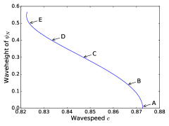
(a)

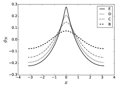
(b)

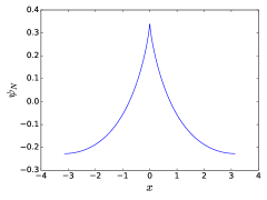
(c)

(d)

Figure 17: (a) Numerical approximation of the bifurcation branch of even, $2\pi$-periodic solutions of (3.19), with with specific points A-E labeled for forthcoming computations: Point A at $c\approx 0.8727$, height $\approx 0.01$; Point B at $c\approx 0.8662$, height $\approx 0.14$; Point C at $c\approx 0.8470$, height $\approx 0.30$; Point D at $c\approx 0.8333$, height $\approx 0.4$; Point E at $c\approx 0.8237$, height $\approx 0.50$. (b) the profiles associated to the sampled points A-E in (a). (c) A (nearly peaked) $2\pi$-periodic profile near the top of the bifurcation branch of $2\pi$-periodic solutions, corresponding to $c\approx 0.8227$, $\text{waveheight}\approx 0.5650$. (d) The bifurcation branches of $2\pi/\kappa$-periodic solutions of (3.19) for varying $\kappa$.

To study the stability of these periodic traveling wave solutions, we again follow the method of Appendix A and define the following bi-infinite matrices whose eigenvalues, after finite-dimensional truncation, approximate the spectrum of the corresponding linearization:

$$\widehat{A}^{\mu}(m,l) =ic\kappa(\mu+l)\delta_{m,l}$$

$$\widehat{B}^{\mu}(m,l) =\delta_{m,l}$$

$$\widehat{C}^{\mu}(m,l) =-2\kappa^{2}(\mu+m)^{2}\widehat{\phi}(m-l)-\kappa^{2}(\mu+l)^{2}\widehat{\mathcal{K}}(\kappa(\mu+l))\delta_{m,l}$$

$$\widehat{D}^{\mu}(m,l) =ic\kappa(\mu+l)\delta_{m,l}.$$

Plots of the spectrum, along with the growth rates $\operatorname{Re}(\lambda)$ with respect to the Bloch parameter $\mu$, are shown in Figures 18 and 19, respectively. Based on these numerics, we see that, similar to the other models considered here, all waves of sufficiently large waveheight appear to exhibit both modulational and high-frequency instabilities, while high-frequency instabilities for asymptotically small waves are unobserved in our experiments. Furthermore, all computed waves appear to be spectrally stable with respect to co-periodic perturbations.

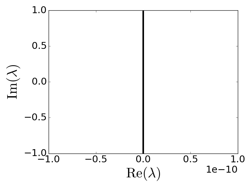
(a)

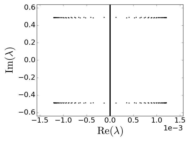
(b)

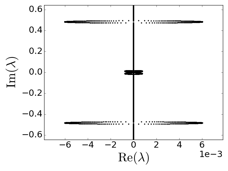
(c)

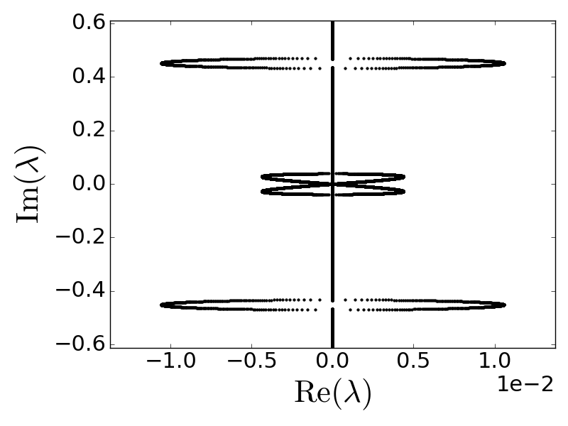
(d)

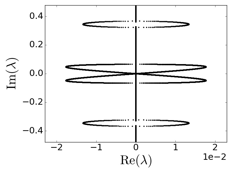
(e)

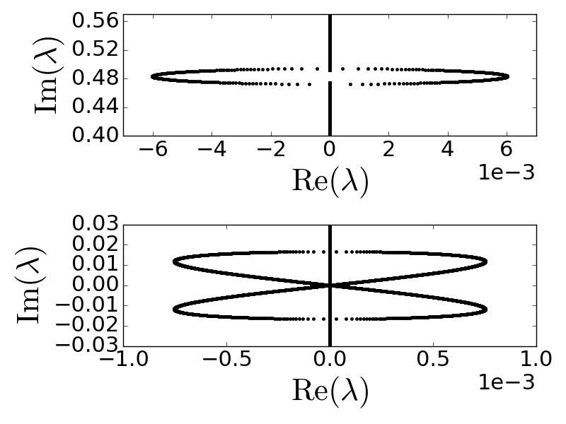
(f)

Figure 18: (a)-(e) Spectral plots for Boussinesq-Whitham at the points A-E, respectively, sampled along the bifurcation branch for $2\pi$-periodic solutions in Figure 17(a). (f) A zoom-in on the high-frequency instability (top) and modulational instability (bottom) for the spectral plot (c).

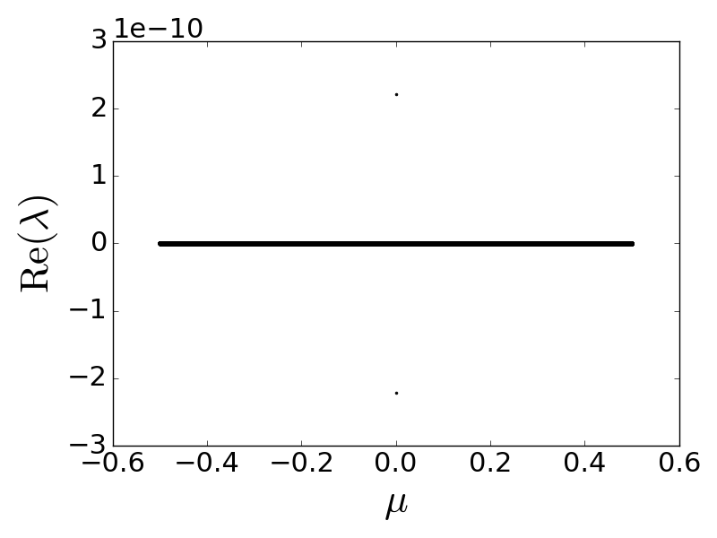
(a)

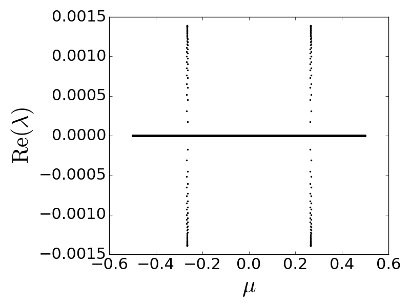
(b)

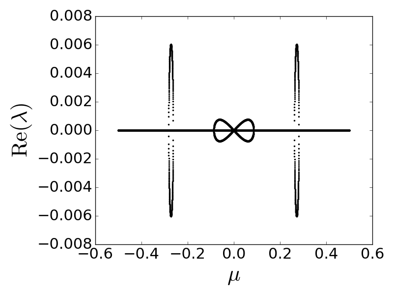
(c)

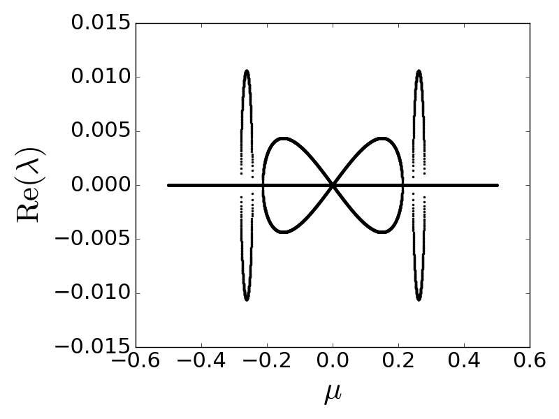
(d)

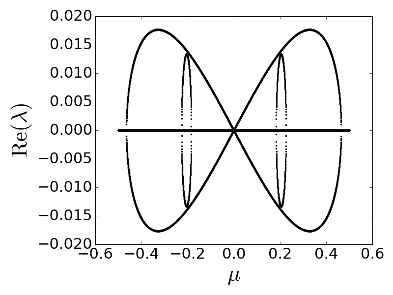
(e)

Figure 19: (a)-(e) $\operatorname{Re}(\lambda)$ vs. $\mu$ for each of the spectral plots (a)-(e), respectively, of Boussinesq-Whitham shown in Figure 18.

4 Conclusion

Using well-conditioned numerical methods, we have presented numerically-computed waveheight vs. wavespeed global bifurcation diagrams for three fully-dispersive bidirectional Whitham models and studied the spectral stability of such waves by numerically approximating the spectrum of their associated linearized operators in both small and large amplitude regimes. Our results confirm a number of analytical results concerning the stability of asymptotically small waves in these models and provide new insight into the existence and stability of large amplitude waves, including highest singular waves. We note that while these models compare similarly with regard to existence and stability, we find evidence that the model (1.4) does not have a highest singular wave. Furthermore, we provide numerical evidence that the conditional well-posedness result in [8] is in fact sharp, in the sense that local evolution of initial data with height profiles with negative minima appears to be ill-posed. This has led us to construct and analyze new wavetrain solutions of (1.2) with strictly positive height profile, ensuring the local dynamics about such waves is indeed well-posed.

Appendix A General Framework for Computing the Spectrum of the Linearization

In this appendix we seek to generalize the method for shown in Section 3.1 for setting up a bi-infinite matrix representation of a linearized operator, whose spectrum is suitably approximated by truncating to finite dimensions.

Recall that we are dealing with nonlinear traveling wave models of the form (1.8). To linearize the operator associated with such a model about an equilibrium solution $(u(x,t),\eta(x,t))=(\phi(x),\psi(x))$, we first express solutions $u$ and $\eta$ as localized perturbations from equilibrium:

$$\begin{array}[]{rcl}u(x,t)&=&\phi(x)+\varepsilon v(x,t)+\mathcal{O}(\varepsilon^{2})\\ \eta(x,t)&=&\psi(x)+\varepsilon w(x,t)+\mathcal{O}(\varepsilon^{2})\end{array}$$ (A.1)

with $v(\cdot,t),w(\cdot,t)\in L^{2}(\mathbb{R})$ for each $t>0$ for which they are defined. Substituting (A.1) into (1.7), Taylor expanding, and taking $\varepsilon\to 0$ yields

$$\left\{\begin{array}[]{rcl}v_{t}&=&\displaystyle\sum_{j=0}^{n}\left[F_{\partial_{x}^{j}u}(\vec{\phi},\vec{\psi})\partial_{x}^{j}v+F_{\partial_{x}^{j}u}(\vec{\phi},\vec{\psi})\partial_{x}^{j}w\right]\\ w_{t}&=&\displaystyle\sum_{j=0}^{n}\left[G_{\partial_{x}^{j}u}(\vec{\phi},\vec{\psi})\partial_{x}^{j}v+G_{\partial_{x}^{j}u}(\vec{\phi},\vec{\psi})\partial_{x}^{j}w\right]\end{array}\right.$$ (A.2)

where

$$\vec{\phi}:=(\phi,\phi^{\prime},\phi^{\prime\prime},\ldots\phi^{(n)}),\quad\vec{\psi}:=(\psi,\psi^{\prime},\psi^{\prime\prime},\ldots\psi^{(n)}).$$

As was done in [22] for the Whitham equation, we will apply Bloch theory to study the $2\pi$-periodic spectrum of the linearization by writing

$$v(x,t)=e^{\lambda t}V(x)+c.c.,\quad w(x,t)=e^{\lambda t}W(x)+c.c.,$$ (A.3)

where $c.c.$ denotes complex conjugate of the preceding expression (in order to ensure the reality of the functions $v$ and $w$), and

$$V(x)=\sum_{l\in\mathbb{Z}}\widetilde{V}(l)e^{i\kappa(\mu+l)x},\quad W(x)=\sum_{l\in\mathbb{Z}}\widetilde{W}(l)e^{i\kappa(\mu+l)x}$$ (A.4)

with Bloch coefficients $\widetilde{V}(l),\widetilde{W}(l)$ for $l\in\mathbb{Z}$ and Bloch parameter $\mu\in[0,1)$. Per equations (A.2), we will need to understand how the operators $F_{\partial_{x}^{j}u}$, $F_{\partial_{x}^{j}\eta}$, $G_{\partial_{x}^{j}u}$, and $G_{\partial_{x}^{j}\eta}$ act on the Bloch decompositions (A.4). In the models of interest, these operators will be linear combinations of $2\pi$-periodic multiplication operators and the (pseudo)differential operators $\mathcal{K},\partial_{x}$. We derive the Bloch transforms of such operators here.

If $f$ is a $2\pi/\kappa$-periodic function (multiplication operator), then we may represent $f$ in Fourier series as

$$f(x)=\sum_{m\in\mathbb{Z}}\widehat{f}(m)e^{im\kappa x}.$$

Then

$$f(x)V(x) =\left(\sum_{m\in\mathbb{Z}}\widehat{f}(m)e^{im\kappa x}\right)\left(\sum_{l\in\mathbb{Z}}\widetilde{V}(l)e^{i\kappa(\mu+l)x}\right)$$

$$=\sum_{m\in\mathbb{Z}}\sum_{l\in\mathbb{Z}}\widehat{f}(m)\widetilde{V}(l)e^{i\kappa(\mu+m+l)x}$$

$$=\sum_{m\in\mathbb{Z}}\left(\sum_{l\in\mathbb{Z}}\widehat{f}(m-l)\widetilde{V}(l)\right)e^{i\kappa(\mu+m)x}\quad\text{by taking $m\mapsto m-l$.}$$

Hence the Bloch transform of the product $fV$ is given by

$$\widetilde{fV}(m)=\sum_{l\in\mathbb{Z}}\widehat{f}(m-l)\widetilde{V}(l),\quad m\in\mathbb{Z}.$$ (A.5)

Moreover, the Bloch transform with parameter $\mu$ acts on the derivative operator $\partial_{x}$ as

$$\widetilde{\partial_{x}f}(m)=\widehat{\partial_{x}}(\kappa(\mu+m))\widetilde{f}(m)=i\kappa(\mu+m)\widetilde{f}(m),\quad m\in\mathbb{Z},$$

and, by analogy, the Bloch transform acts on the pseudodifferential operator $\mathcal{K}$ as

$$\widetilde{\mathcal{K}f}(m):=\widehat{\mathcal{K}}(\kappa(\mu+m))\widetilde{f}(m)=\frac{\tanh(\kappa(\mu+m))}{\kappa(\mu+m)}\widetilde{f}(m),\quad m\in\mathbb{Z}.$$ (A.6)

Substituting (A.3) into (A.2) and taking the Bloch transform of both sides, we have the simultaneous eigenvalue problems

$$\lambda\widetilde{V}(m) =\sum_{j=0}^{n}\left(F_{\partial_{x}^{j}u}(\vec{\phi},\vec{\psi};c)V^{(j)}+F_{\partial_{x}^{j}\eta}(\vec{\phi},\vec{\psi};c)W^{(j)}\right)^{\sim}(m)$$

$$=:\sum_{l\in\mathbb{Z}}\left[\widehat{A}^{\mu}(m,l)\widetilde{V}(l)+\widehat{B}^{\mu}(m,l)\widetilde{W}(l)\right]$$ (A.7)

$$\text{and}\quad\lambda\widetilde{W}(m) =\sum_{j=0}^{n}\left(G_{\partial_{x}^{j}u}(\vec{\phi},\vec{\psi};c)V^{(j)}+G_{\partial_{x}^{j}\eta}(\vec{\phi},\vec{\psi};c)W^{(j)}\right)^{\sim}(m)$$

$$=:\sum_{l\in\mathbb{Z}}\left[\widehat{C}^{\mu}(m,l)\widetilde{V}(l)+\widehat{D}^{\mu}(m,l)\widetilde{W}(l)\right],$$ (A.8)

where $\widehat{A}^{\mu}(m,l)$, $\widehat{B}^{\mu}(m,l)$, $\widehat{C}^{\mu}(m,l)$, and $\widehat{D}^{\mu}(m,l)$ are the coefficients of the Bloch coefficients upon expanding the Bloch transform. Define the following bi-infinite matrices entry-wise for row-$m$ and column-$l$ with $m,l\in\mathbb{Z}$ as

$$\widehat{A}^{\mu}:=[\widehat{A}^{\mu}(m,l)]_{m,l\in\mathbb{Z}},\quad\widehat{B}^{\mu}:=[\widehat{B}^{\mu}(m,l)]_{m,l\in\mathbb{Z}},\quad\widehat{C}^{\mu}:=[\widehat{C}^{\mu}(m,l)]_{m,l\in\mathbb{Z}},\quad\widehat{D}^{\mu}:=[\widehat{D}^{\mu}(m,l)]_{m,l\in\mathbb{Z}}.$$ (A.9)

Writing (A.7) and (A.8) jointly in block bi-infinte matrix form, we have

$$\lambda\left[\begin{array}[]{c}\widetilde{V}\\ \hline\cr\widetilde{W}\end{array}\right]=\left[\begin{array}[]{c|c}\widehat{A}^{\mu}&\widehat{B}^{\mu}\\ \hline\cr\widehat{C}^{\mu}&\widehat{D}^{\mu}\end{array}\right]\left[\begin{array}[]{c}\widetilde{V}\\ \hline\cr\widetilde{W}\end{array}\right]=:\widehat{\mathcal{L}}^{\mu}\left[\begin{array}[]{c}\widetilde{V}\\ \hline\cr\widetilde{W}\end{array}\right]$$ (A.10)

where

$$\widetilde{V} :=\begin{bmatrix}\ldots&\widetilde{V}(-2)&\widetilde{V}(-1)&\widetilde{V}(0)&\widetilde{V}(1)&\widetilde{V}(2)&\ldots\end{bmatrix}^{T}$$

$$\widetilde{W} :=\begin{bmatrix}\ldots&\widetilde{W}(-2)&\widetilde{W}(-1)&\widetilde{W}(0)&\widetilde{W}(1)&\widetilde{W}(2)&\ldots\end{bmatrix}^{T}.$$

To numerically approximate the bi-infinite eigenvalue problem (A.10), we truncate each of the bi-infinite matrices $\widehat{A}^{\mu}$, $\widehat{B}^{\mu}$, $\widehat{C}^{\mu}$, and $\widehat{D}^{\mu}$ to have dimension $(2N+1)\times(2N+1)$, i.e.

$$\widehat{A}_{N}^{\mu}(m,l):=[\widehat{A}^{\mu}(m,l)]_{-N\leq m,l\leq N}\in\mathbb{C}^{(2N+1)\times(2N+1)}$$

and similarly define $\widehat{B}_{N}^{\mu}$, $\widehat{C}_{N}^{\mu}$, and $\widehat{D}_{N}^{\mu}$, which together form $\widehat{\mathcal{L}}_{N}^{\mu}\in\mathbb{C}^{(4N+2)\times(4N+2)}$ as shown in (A.11) below. Moreover, we also truncate $\widetilde{V}$ and $\widetilde{W}$ as

$$\widetilde{V}_{N}=\begin{bmatrix}\widetilde{V}(-N)&\ldots&\widetilde{V}(0)&\ldots&\widetilde{V}(N)\end{bmatrix}^{T},\quad\widetilde{W}_{N}=\begin{bmatrix}\widetilde{W}(-N)&\ldots&\widetilde{W}(0)&\ldots&\widetilde{W}(N)\end{bmatrix}^{T}.$$

Then, using a standard matrix eigenvalue solver (e.g. Matlab’s eig or Python’s numpy.linalg.eig [15]), we solve for $\lambda_{N}^{\mu}\in\mathbb{C}$ such that

$$\lambda_{N}^{\mu}\left[\begin{array}[]{c}\widetilde{V}_{N}\\ \hline\cr\widetilde{W}_{N}\end{array}\right]=\left[\begin{array}[]{c|c}\widehat{A}_{N}^{\mu}&\widehat{B}_{N}^{\mu}\\ \hline\cr\widehat{C}_{N}^{\mu}&\widehat{D}_{N}^{\mu}\end{array}\right]\left[\begin{array}[]{c}\widetilde{V}_{N}\\ \hline\cr\widetilde{W}_{N}\end{array}\right]=:\widehat{\mathcal{L}}^{\mu}_{N}\left[\begin{array}[]{c}\widetilde{V}_{N}\\ \hline\cr\widetilde{W}_{N}\end{array}\right]$$ (A.11)

We solve this eigenvalue problem for $\mu$ in a discrete subset of $[0,1)$. For our computations, we used a uniform mesh $\{\mu_{j}=j\Delta\mu\}_{j}$ with subintervals of constant width $\Delta\mu$.

Remark A.1.

The above method is inspired by the Fourier-Floquet-Hill Method (FFHM) given in [3], which is used to compute the spectrum of a linear, locally-acting operator having periodic coefficients. As was done in [3], we define convergence of the spectral approximation in the sense that any eigenvalue $\lambda_{N}^{\mu}$ of $\widehat{\mathcal{L}}_{N}^{\mu}$ above converges to some eigenvalue $\lambda$ of non-truncated linearization $\mathcal{L}$. Moreover, the incorporation of all Bloch parameters $\mu\in[0,1)$ yields the entire spectrum, i.e.

$$\lim_{N\to\infty}\bigcup_{\mu\in[0,1)}\sigma(\widehat{\mathcal{L}}_{N}^{\mu})=\sigma(\mathcal{L}).$$

To obtain the approximate Fourier coefficients $\widehat{\phi}$ and $\widehat{\psi}$ (in the exponential basis) needed to construct the bi-infinite matrix $\widehat{\mathcal{L}}_{N}^{\mu}$, for a given wavespeed $c$, we use the approximate values of $\phi(x_{m})$ at each collocation point $x_{m}=\frac{(2m-1)\pi}{2\kappa N}$ obtained in the numerical bifurcation (see Section 2) and compute the approximate coefficients via their integral definitions using the midpoint quadrature:

$$\widehat{\phi}(n) =\frac{\kappa}{2\pi}\int_{-\pi/\kappa}^{\pi/\kappa}\phi(x)e^{-in\kappa x}\,dx$$

$$=\frac{\kappa}{\pi}\int_{0}^{\pi/\kappa}\phi(x)\cos(n\kappa x)\,dx\quad\text{since $\phi$ is even}$$

$$\approx\frac{1}{N}\sum_{m=1}^{N}\phi(x_{m})\cos(n\kappa x_{m})\quad\text{by \eqref{E:fourier_integral_discretization}.}$$

Similarly,

$$\widehat{\psi}(n)\approx\frac{1}{N}\sum_{m=1}^{N}\psi(x_{m})\cos(n\kappa x_{m}).$$

Remark A.2.

The approximation of $\widehat{\psi}(n)$ above requires that $\psi$ be an even function. This is always the case since we are considering models for which $\psi$ can be resolved in terms of $\phi$, hence $\psi=\psi(\phi(x))$ is also an even function.

As an example, here we show the relevant calculations in detail for the model (3.1) as a concrete demonstration of the more abstract framework established in this appendix. Recall that this model is given by

$$\left\{\begin{array}[]{rcl}u_{t}&=&cu_{x}-\eta_{x}-uu_{x}=:F(u,u_{x},\eta,\eta_{x})\\ \eta_{t}&=&c\eta_{x}-\mathcal{K}u_{x}-(\eta u)_{x}=:G(u,u_{x},\eta,\eta_{x}),\end{array}\right.$$

with equilibrium solutions $u(x,t)=\phi(x)$, $\eta(x,t)=\psi(x)$. Beginning with (3.11), we first compute

$$F_{u}(\phi,\phi^{\prime},\psi,\psi^{\prime})=-\phi^{\prime},\quad F_{u_{x}}(\phi,\phi^{\prime},\psi,\psi^{\prime})=c-\phi,\quad F_{\eta}(\phi,\phi^{\prime},\psi,\psi^{\prime})=0,\quad F_{\eta_{x}}(\phi,\phi^{\prime},\psi,\psi^{\prime})=-1.$$

All of the above are $2\pi/\kappa$-periodic multiplication operators, hence we apply (A.5) in (A.7), here with $n=1$, to achieve the following formulas for $m\in\mathbb{Z}$:

$$\widetilde{F_{u}V}(m) =\sum_{l\in\mathbb{Z}}\widehat{-\phi^{\prime}}(m-l)\widetilde{V}(l)=\sum_{l\in\mathbb{Z}}-i\kappa(m-l)\widehat{\phi}(m-l)\widetilde{V}(l)$$

$$\widetilde{F_{u_{x}}V^{\prime}}(m) =\sum_{l\in\mathbb{Z}}\widehat{(c-\phi)}(m-l)\ \widetilde{\partial_{x}V}(l)=\sum_{l\in\mathbb{Z}}\left(c\delta_{m,l}-\widehat{\phi}(m-l)\right)\cdot i\kappa(\mu+l)\widetilde{V}(l)$$

$$\widetilde{F_{\eta}W}(m) =\sum_{l\in\mathbb{Z}}0\,\widetilde{W}(l)$$

$$\widetilde{F_{\eta_{x}}W^{\prime}}(m) =\sum_{l\in\mathbb{Z}}\widehat{(-1)}(m-l)\ \widetilde{\partial_{x}W}(l)=\sum_{l\in\mathbb{Z}}-\delta_{m,l}\cdot i\kappa(\mu+l)\widetilde{W}(l),$$

where $\delta_{m,l}$ is the Kronecker delta. Summing the above expressions and grouping terms involving $\widetilde{V}(l)$ and $\widetilde{W}(l)$ per (A.7), we obtain

$$\widehat{A}^{\mu}(m,l) =-i\kappa(m-l)\widehat{\phi}(m-l)+\left(c\delta_{m,l}-\widehat{\phi}(m-l)\right)\cdot i\kappa(\mu+l)$$

$$=ic\kappa(\mu+l)\delta_{m,l}-i\kappa(\mu+m)\widehat{\phi}(m-l)$$ (A.12)

$$\widehat{B}^{\mu}(m,l) =-i\kappa(\mu+l)\delta_{m,l},$$ (A.13)

Similarly, per (A.8), we compute

$$G_{u}(\phi,\phi^{\prime},\psi,\psi^{\prime})=-\psi^{\prime},\quad G_{u_{x}}(\phi,\phi^{\prime},\psi,\psi^{\prime})=-\mathcal{K}-\psi,\quad G_{\eta}(\phi,\phi^{\prime},\psi,\psi^{\prime})=-\phi^{\prime},\quad G_{\eta_{x}}(\phi,\phi^{\prime},\psi,\psi^{\prime})=c-\phi.$$

Then

$$\widetilde{G_{u}V}(m) =\sum_{l\in\mathbb{Z}}\widehat{-\psi^{\prime}}(m-l)\widetilde{V}(l)=-i\kappa(m-l)\widehat{\psi}(m-l)\widetilde{V}(l)$$

$$\widetilde{G_{u_{x}}V^{\prime}}(m) =\left[(-\mathcal{K}-\psi)\partial_{x}V\right]^{\sim}(m)$$

$$=-\widetilde{\mathcal{K}\partial_{x}V}(m)-\widetilde{\psi\,\partial_{x}V}(m)$$

$$=-i\kappa(\mu+m)\widehat{\mathcal{K}}(\kappa(\mu+m))\widetilde{V}(m)-\sum_{l\in\mathbb{Z}}\widehat{\psi}(m-l)\,i\kappa(\mu+l)\widetilde{V}(l)$$

$$=\sum_{l\in\mathbb{Z}}-i\kappa(\mu+l)\left[\widehat{\mathcal{K}}(\kappa(\mu+l))\delta_{m,l}+\widehat{\psi}(m-l)\right]\widetilde{V}(l)$$

$$\widetilde{G_{\eta}W}(m) =\sum_{l\in\mathbb{Z}}\widehat{-\phi^{\prime}}(m-l)\widetilde{W}(l)=\sum_{l\in\mathbb{Z}}-i\kappa(m-l)\widehat{\phi}(m-l)\widetilde{W}(l)$$

$$\widetilde{G_{\eta_{x}}W^{\prime}}(m) =\sum_{l\in\mathbb{Z}}\widehat{(c-\phi)}(m-l)\ \widetilde{\partial_{x}W}(l)=\sum_{l\in\mathbb{Z}}\left(c\delta_{m,l}-\widehat{\phi}(m-l)\right)\cdot i\kappa(\mu+l)\widetilde{W}(l).$$

Summing the above expressions and grouping terms involving $\widetilde{V}(l)$ and $\widetilde{W}(l)$ per (A.8), we obtain

$$\widehat{C}^{\mu}(m,l) =-i\kappa(\mu+l)\widehat{\mathcal{K}}(\kappa(\mu+l))\delta_{m,l}-i\kappa(\mu+m)\widehat{\psi}(m-l)$$ (A.14)

$$\widehat{D}^{\mu}(m,l) =ic\kappa(\mu+l)\delta_{m,l}-i\kappa(\mu+m)\widehat{\phi}(m-l).$$ (A.15)

Note that the formulas for $\widehat{A}^{\mu}(m,l)$, $\widehat{B}^{\mu}(m,l)$, $\widehat{C}^{\mu}(m,l)$, $\widehat{D}^{\mu}(m,l)$ given above in (A.12), (A.13), (A.14), and (A.15) agree with those found in Section 3.1 circa (3.11), (3.12) by manipulating Fourier series.

Appendix B Numerical Parameters

B.1 Bifurcation and Spectral Figures

In Table 1, we provide the numerical parameters used to compute bifurcations via the pseudoarclength method and spectra via the Fourier-Floquet-Hill-Method (FFHM). A brief reminder of the symbols involved:

Pseudoarclength Parameters:

• $\kappa$ is the wavenumber, which yields waves of period $2\pi/\kappa$.

• $N$ is the number of collocation points $x_{i}=\frac{(2i-1)\pi}{2\kappa N}$, $i=1,\ldots,N$ on the half-period cell $[0,\pi/\kappa]$, as well as the number of modes used in the profile’s truncated series $\phi(x)=\sum_{n=0}^{N-1}\widehat{\phi}(n)\cos(n\kappa x)$. See Section 2.1.

• $h$ is the length of a step along the tangent direction in each iteration of the pseudoarclength method. See Figure 1 and the surrounding discussion.

• $\varepsilon_{0}$ determines a suitable starting point (see (2.11)) near the global bifurcation curve based on the model’s local bifurcation formulas (e.g. (3.5), (3.5)).

FFHM Parameters:

• $\Delta\mu$ is the width of a subinterval in the uniform mesh $\{\mu_{j}=j\Delta\mu\}_{j}\subset[0,1)$ of Bloch parameters used to discretize the $L^{2}(\mathbb{R})$ spectrum. See (A.4) and Remark A.1.

• $N$ determines the dimension of the truncated bi-infinite matrix $\widehat{\mathcal{L}}_{N}^{\mu}\in\mathbb{C}^{(4N+2)\times(4N+2)}$. See (A.11) and the surrounding discussion.

Table 1: Parameters for figures generated by the pseudoarclength method (bifurcation) and Fourier-Floquet-Hill method (spectrum).

Figure(s)	Psuedoarclength Parameters	FFHM Parameters (if applicable)
2 (a)	$\kappa=1$, $N=256$, $h=0.001$, $\varepsilon_{0}=1\times 10^{-5}$
2 (b)	$\kappa\in\{0.8,1.0,1.3,1.6\}$, $N=256$, $h=0.001$, $\varepsilon_{0}=1\times 10^{-5}$
3 (a), (b)	$\kappa=1$, $N=256$, $h=0.001$, $\varepsilon_{0}=1\times 10^{-5}$
4 (a)	$\kappa=1$, $N=256$, $h=0.001$, $\varepsilon_{0}=1\times 10^{-5}$	$N=50$, $\Delta\mu=1/10000$
4 (b), (c)	$\kappa=1$, $N=256$, $h=0.001$, $\varepsilon_{0}=1\times 10^{-5}$	$N=50$, $\Delta\mu=1/5000$
4 (d), (e)	$\kappa=1$, $N=256$, $h=0.001$, $\varepsilon_{0}=1\times 10^{-5}$	$N=128$, $\Delta\mu=1/5000$
5 (a)-(e)	Same data as Figure 4 (a)-(e)	Same data as Figure 4 (a)-(e)
6 (a)	$\kappa=1.005$, $N=64$, $h=0.001$, $\varepsilon_{0}=1\times 10^{-5}$	$N=50$, $\Delta\mu=1/15000$
6 (b)	$\kappa=1.008$, $N=64$, $h=0.001$, $\varepsilon_{0}=1\times 10^{-5}$	$N=64$, $\Delta\mu=1/15000$
8 (b)	$\kappa\in\{0.5,1.0,1.3,1.6\}$, $N=256$, $h=0.001$, $\varepsilon_{0}=1\times 10^{-5}$
9 (a), (b)	$\kappa=1$, $N=2048$, $h=0.001$, $\varepsilon_{0}=1\times 10^{-5}$
11 (a)	$\kappa=1$, $N=2048$, $h=0.001$, $\varepsilon_{0}=1\times 10^{-5}$	$N=50$, $\Delta\mu=1/50000$
11 (b)	$\kappa=1$, $N=2048$, $h=0.001$, $\varepsilon_{0}=1\times 10^{-5}$	$N=50$, $\Delta\mu=1/10000$
11 (c)	$\kappa=1$, $N=2048$, $h=0.001$, $\varepsilon_{0}=1\times 10^{-5}$	$N=128$, $\Delta\mu=1/5000$
12 (a)-(c)	$\kappa=1.611$, $N=256$, $h=0.001$, $\varepsilon_{0}=1\times 10^{-5}$
12 (d)	$\kappa\in\{0.8,1,1.3,1.6\}$, $N=256$, $h=0.001$, $\varepsilon_{0}=1\times 10^{-5}$
13	$\kappa=1$, $N\in\{64,128,256,512\}$, $h=0.001$, $\varepsilon_{0}=1\times 10^{-5}$
14 (a), (b)	$\kappa=1.611$, $N=256$, $h=0.001$, $\varepsilon_{0}=1\times 10^{-5}$	$N=50$, $\Delta\mu=1/10000$
14 (c), (d)	$\kappa=1.611$, $N=256$, $h=0.001$, $\varepsilon_{0}=1\times 10^{-5}$	$N=50$, $\Delta\mu=1/5000$
14 (e)	$\kappa=1.611$, $N=256$, $h=0.001$, $\varepsilon_{0}=1\times 10^{-5}$	$N=128$, $\Delta\mu=1/5000$
15 (a), (b)	$\kappa=1.609$, $N=256$, $h=0.001$, $\varepsilon_{0}=1\times 10^{-5}$	$N=50$, $\Delta\mu=1/10000$
16 (a)-(e)	Same data as Figure 14	Same data as Figure 14
17 (a)-(c)	$\kappa=1$, $N=256$, $h=0.001$, $\varepsilon_{0}=1\times 10^{-5}$
17 (d)	$\kappa\in\{0.8,1.0,1.3,1.6\}$, $N=256$, $h=0.001$, $\varepsilon_{0}=1\times 10^{-5}$
18 (a)-(d)	$\kappa=1$, $N=256$, $h=0.001$, $\varepsilon_{0}=1\times 10^{-5}$	$N=50$, $\Delta\mu=1/10000$
18 (e)	$\kappa=1$, $N=256$, $h=0.001$, $\varepsilon_{0}=1\times 10^{-5}$	$N=128$, $\Delta\mu=1/10000$
19	Same data as Figure 18	Same data as Figure 18

B.2 Time Evolution

We use a sixth-order pseudospectral operator splitting method [25] to evolve a traveling wave solution of (1.2) by successively evolving the linear and nonlinear parts of the system. The linear part of (1.2) is

$$\left\{\begin{array}[]{rcl}u_{t}&=&-\eta_{x}\\ \eta_{t}&=&-\mathcal{K}u_{x},\end{array}\right.$$

which can be transformed into decoupled wave-like second-order in time IVPs

$$\left\{\begin{array}[]{rcl}\eta_{tt}(x,t)&=&\mathcal{K}\eta_{xx}(x,t)\\ \eta(x,0)&=&\psi(x)\\ \eta_{t}(x,0)&=&-\mathcal{K}\phi^{\prime}(x)\end{array}\right.\quad\left\{\begin{array}[]{rcl}u_{tt}(x,t)&=&\mathcal{K}u_{xx}(x,t)\\ u(x,0)&=&\phi(x)\\ u_{t}(x,0)&=&-\psi^{\prime}(x),\end{array}\right.$$

where $\psi(x)$, $\phi(x)$ are equilibria as discussed in Section 3.1. Taking the Fourier transform of the above equations in $x$ yields ODE IVPs in $t$ for each fixed $n\in\mathbb{Z}$:

$$\left\{\begin{array}[]{rcl}\widehat{\eta}_{tt}(n,t)&=&-\kappa^{2}n^{2}\widehat{\mathcal{K}}(n)\widehat{\eta}(n,t)\\ \widehat{\eta}(n,0)&=&\widehat{\psi}(n)\\ \widehat{\eta}_{t}(n,0)&=&-in\widehat{\mathcal{K}}(n)\widehat{\phi}(n)\end{array}\right.\quad\left\{\begin{array}[]{rcl}\widehat{u}_{tt}(n,t)&=&-\kappa^{2}n^{2}\widehat{\mathcal{K}}(n)\widehat{u}(n,t)\\ \widehat{u}(n,0)&=&\widehat{\phi}(n)\\ \widehat{u}_{t}(n,0)&=&-in\widehat{\psi}(n).\end{array}\right.$$ (B.1)

The equations in (B.1) are well-known to model simple harmonic motion and can be solved explicitly. For the nonlinear part of (1.2), the typical fourth-order Runge-Kutta scheme (RK4) is used.

• In Figure 7, a small $2\pi$-periodic wave of height $\max\psi-\min\psi\approx 0.00109$ generated by the pseudoarclength method with parameters $\kappa=1$, $h=0.01$, $\varepsilon_{0}=1\times 10^{-5}$, and $N=2048$ collocation points on the half-periodic cell $[0,\pi]$ ($\Delta x=\frac{\pi}{2048}\approx 0.00153$) is used as initial data in (B.1). A time step of $\Delta t=0.001$ is used in each iteration of the 6th-order operator splitting method to integrate to time $t=2.55$, which is about 35.4% of a temporal period for this wave.

• In Figure 10, a large $2\pi$-periodic positive wave of height $\max\psi-\min\psi\approx 0.387$ generated by the pseudoarclength method with parameters $\kappa=1$, $h=0.01$, $\varepsilon_{0}=1\times 10^{-5}$, and $N=2048$ collocation points on the half-periodic cell $[0,\pi]$ ($\Delta x=\frac{\pi}{2048}\approx 0.00153$) is used as initial data in (B.1). A time step of $\Delta t=0.001$ was used to integrate for 15 temporal periods (to time $t\approx 80.5706$).

The ease of time-evolving large positive waves (which are proven to be locally well-posed; see [8]), as opposed to the difficulty of evolving non-positive waves in the same model with the same $\Delta t/\Delta x\approx 0.6536$ suggests that the non-positive waves are not locally well-posed in time.

References

- [1] Jared C. Bronski, Vera Mikyoung Hur, and Mathew A. Johnson. Modulational instability in equations of KdV type. In New approaches to nonlinear waves, volume 908 of Lecture Notes in Phys., pages 83–133. Springer, Cham, 2016.
- [2] J. D. Carter. Bidirectional Whitham Equations as Models of Waves on Shallow Water. ArXiv e-prints, May 2017. arXiv:1705.06503.
- [3] Bernard Deconinck and J. Nathan Kutz. Computing spectra of linear operators using the floquet–fourier–hill method. Journal of Computational Physics, 219(1):296 – 321, 2006.
- [4] Bernard Deconinck and Katie Oliveras. The instability of periodic surface gravity waves. J. Fluid Mech., 675:141–167, 2011.
- [5] Bernard Deconinck and Olga Trichtchenko. High-frequency instabilities of small-amplitude solutions of Hamiltonian PDEs. Discrete Contin. Dyn. Syst., 37(3):1323–1358, 2017.
- [6] M. Ehrnström, M. A. Johnson, and K. M. Claassen. Existence of a highest wave in a fully dispersive two-way shallow water model. ArXiv e-prints, October 2016. arXiv:1610.02603.
- [7] M. Ehrnström and H. Kalisch. Global bifurcation for the Whitham equation. Math. Model. Nat. Phenom., 8(5):13–30, 2013.
- [8] M. Ehrnström, L. Pei, and Y. Wang. A conditional well-posedness result for the bidirectional Whitham equation. ArXiv e-prints, August 2017. arXiv:1708.04551.
- [9] M. Ehrnström and E. Wahlén. On whitham’s conjecture of a highest cusped wave for a nonlocal dispersive shallow water wave equation. Preprint, 2015. arXiv:1602.05384.
- [10] Mats Ehrnström and Henrik Kalisch. Traveling waves for the Whitham equation. Differential Integral Equations, 22(11-12):1193–1210, 2009.
- [11] V. Mikyoung Hur and A. K. Pandey. Modulational instability in a full-dispersion shallow water model. ArXiv e-prints, August 2016. arXiv:1608.04685.
- [12] Vera Mikyoung Hur. Wave breaking in the Whitham equation. Adv. Math., 317:410–437, 2017.
- [13] Vera Mikyoung Hur and Mathew A. Johnson. Modulational instability in the Whitham equation for water waves. Stud. Appl. Math., 134(1):120–143, 2015.
- [14] Vera Mikyoung Hur and Mathew A. Johnson. Modulational instability in the Whitham equation with surface tension and vorticity. Nonlinear Anal., 129:104–118, 2015.
- [15] Eric Jones, Travis Oliphant, Pearu Peterson, et al. SciPy: Open source scientific tools for Python, 2001–.
- [16] John W. McLean. Instabilities of finite-amplitude gravity waves on water of finite depth. J. Fluid Mech., 114:331–341, 1982.
- [17] Dimitrios Mitsotakis, Denys Dutykh, and John Carter. On the nonlinear dynamics of the traveling-wave solutions of the Serre system. Wave Motion, 70:166–182, 2017.
- [18] Daulet Moldabayev, Henrik Kalisch, and Denys Dutykh. The Whitham equation as a model for surface water waves. Phys. D, 309:99–107, 2015.
- [19] A. K. Pandey. Comparison of modulational instabilities in full-dispersion shallow water models. ArXiv e-prints, August 2017. arXiv:1708.00547.
- [20] Michael Reed and Barry Simon. Methods of modern mathematical physics. IV. Analysis of operators. Academic Press [Harcourt Brace Jovanovich, Publishers], New York-London, 1978.
- [21] Filippo Remonato and Henrik Kalisch. Numerical bifurcation for the capillary Whitham equation. Phys. D, 343:51–62, 2017.
- [22] Nathan Sanford, Keri Kodama, John D. Carter, and Henrik Kalisch. Stability of traveling wave solutions to the whitham equation. Physics Letters A, 378(30–31):2100 – 2107, 2014.
- [23] Jean-Claude Saut, Chao Wang, and Li Xu. The Cauchy problem on large time for surface-waves-type Boussinesq systems II. SIAM J. Math. Anal., 49(4):2321–2386, 2017.
- [24] G. B. Whitham. Linear and nonlinear waves. Wiley-Interscience [John Wiley & Sons], New York-London-Sydney, 1974. Pure and Applied Mathematics.
- [25] Haruo Yoshida. Construction of higher order symplectic integrators. Phys. Lett. A, 150(5-7):262–268, 1990.