X-ray reflection from cold white dwarfs in magnetic cataclysmic variables

Abstract

We model X-ray reflection from white dwarfs (WD) in magnetic cataclysmic variables (mCVs) with a Monte Carlo simulation. A point source with a power-law spectrum or a realistic post-shock accretion column (PSAC) source irradiates a cool and spherical WD. The PSAC source emits thermal spectra of various temperatures stratified along the column according to the PSAC model. In the point source simulation, we confirm (1) a source harder and nearer to the WD enhances the reflection, (2) higher iron abundance enhances the equivalent widths (EWs) of fluorescent iron K$\alpha_{1,2}$ lines and their Compton shoulder, and increases cut-off energy of a Compton hump, and (3) significant reflection appears from an area that is more than 90^∘ apart from the position right under the point X-ray source because of the WD curvature. The PSAC simulation reveals that (1) a more massive WD basically enhances the intensities of the fluorescent iron K$\alpha_{1,2}$ lines and the Compton hump, except for some specific accretion rate, because the more massive WD makes the hotter PSAC from which higher energy X-rays are preferentially emitted, (2) a larger specific accretion rate monotonically enhances the reflection because it makes the hotter and shorter PSAC, and (3) the intrinsic thermal component hardens by occultation of the cool base of the PSAC by the WD. We quantitatively evaluate influences of the parameters on the EWs and the Compton hump with both types of sources. We also calculate X-ray modulation profiles brought about by the WD spin. They depend on angles of the spin axis from the line of sight and from the PSAC, and whether the two PSACs can be seen. The reflection spectral model and the modulation model involve the fluorescent lines and the Compton hump and can directly be compared to the data which allow us to evaluate these geometrical parameters with unprecedented accuracy.

1 Introduction

A magnetic cataclysmic variable (mCV) is a close binary system which is composed of a Roche Lobe-filling late type star and a highly magnetized ($B>$ 0.1 MG) white dwarf (WD). The mCV is divided into two subclass, that is, a polar and an intermediate polar (IP). In the polar and the IP, the WD magnetic field strength is $0.1<B<10$ MG and $10<B<230$ MG, respectively. In the IP, accreting matter from the companion star forms an accretion disc by its angular momentum. Because the magnetic field of the WD is moderately strong, the accretion disc is disrupted and the accreting matter is caught by the WD magnetic field within the Alfv$\acute{\rm e}$n radius. On the other hand, in the polar, the magnetic field is strong enough to make the WD synchronously rotate with the orbital motion and make the Alfv$\acute{\rm e}$n radius larger than the inner Lagrangian point, and hence the accreting matter overflown from the Lagrangian point is directly caught by the WD magnetic field and the accretion disc is not formed. The accreting matter caught by the magnetic field falls along the line of the magnetic field, undergoes a strong shock and is highly ionized. The generated plasma is hot enough to emit X-rays and is cooled via radiation as it approaches the WD surface. This plasma flow is called a Post-Shock Accretion Column (PSAC).

The PSAC structure and its X-ray spectrum have been considerably modeled (e.g. Hōshi 1973, Aizu 1973, Imamura & Durisen 1983, Wu, Chanmugam, & Shaviv 1994, Woelk & Beuermann 1996, Cropper, Ramsay, & Wu 1998, Cropper et al. 1999, Canalle et al. 2005, Saxton et al. 2005, Saxton et al. 2007 and Hayashi & Ishida 2014a) and some of their X-ray spectral models were applied to observations (e.g. Ramsay et al. 2000, Suleimanov, Revnivtsev, & Ritter 2005, Brunschweiger et al. 2009, Yuasa et al. 2010 and Hayashi & Ishida 2014b). The PSAC structure models were constructed by hydrodynamics. Physical effects such as release of the gravitational potential, non-equipartition between electrons and ions, ionization non-equilibrium, cyclotron cooling, energy conversion between thermal and kinetic energies by variation of the PSAC cross section, or variation of accretion rate per unit area were taken into account. We note that the accretion rate per unit area is often called ’specific accretion rate’ or ’$a$’ in g cm^-2 s^-1. The X-ray spectral models of the PSAC were constructed with distributions of physical quantities of such as temperature calculated by the corresponding PSAC models.

Although, by contrast, X-rays reflected by the WD surface are another important component of the mCV spectrum, it is insufficiently modeled. The reflected X-rays contaminate the intrinsic thermal spectrum, having a spectrum experiencing an energy-dependent modification from the intrinsic one, and make it difficult to extract physical parameters, for example the WD mass. Moreover, the reflection contains important information of the PSAC geometry such as the height of the PSAC and the viewing angle from the PSAC (Hayashi et al. 2011, the angle $i$ in figure 1). The reflection especially forms the fluorescent iron K$\alpha_{1,2}$ lines and their Compton shoulder around 6 keV and Compton hump around 10–50 keV (e.g. George & Fabian 1991). The features are intense and become comparable to the intrinsic thermal component. We can extract information of the PSAC structure and the viewing angle by careful spectral modeling of the reflection because the intensity and the spectral shape of the reflection depend on them.

We therefore construct a spectral model of the reflection using a Monte Carlo simulation. We assume a point source with a power-law spectrum and a realistic PASC source which has finite height and distributions of physical quantities calculated by Hayashi & Ishida (2014a). A cool and spherical WD and occultation by the limb of the WD is also considered.

This paper is organized as follows. We define the framework of our Monte Carlo simulation in section 2. In section 3 and 4, calculation results are shown with the point and the PSAC sources, respectively. We discuss application of the reflection to observations using our results in section 5. Finally, we summarize our results in section 6.

2 Modeling and Calculation

In this section, we describe the framework for our Monte Carlo simulation to model the X-ray spectrum reflected by the WD surface in the mCVs.

2.1 X-ray source

Two types of X-ray sources are assumed in our simulation, that is, the point source (§3) and the realistic PSAC source (§4). The energy range of the X-ray photons used in the simulation is 1–500 keV. The photon number follows a power law of the energy $E$ with the power index ${\it\Gamma}$,

$$N_{0}(E)\propto E^{-{\it\Gamma}}\,{\rm photons\,keV}^{-1}.$$ (1)

The point source is away from the WD surface by $h$ as shown in figure 1 and isotropically emits X-rays.

The PSAC source is a pole of the thin thermal plasma which has finite height of $h$ (figure 1) and negligible cross section. The temperature and the emission measure vary along the pole following the hydrodynamical calculation of the dipolar PSAC calculated by Hayashi & Ishida (2014a). The PSAC is divided into one hundred segments of logarithmically even interval. Each piece irradiates the WD surface with one-temperature thin thermal plasma emission spectrum weighted by its emission measure. The one-temperature spectrum is calculated by SPEX package ver 2.05.04 (Kaastra, Mewe, & Nieuwenhuijzen, 1996).

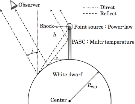
Figure 1: Cross sectional view of a mass accreting magnetic WDs in the mCVs. We adopted two types of X-ray sources: one is point source (dotted circle) whose spectrum follows a power-law function and the other is the PSAC source (gradated gray column) which has finite length and emits multi-temperature thermal plasma spectrum based on the calculation by Hayashi & Ishida (2014a). Dash-dotted and dashed lines show the X-ray paths toward the observer directly from the sources and reflected by the WD surface, respectively. $h$ is distance from the WD surface for the point source and the shock height for the PSAC source. $i$ is called viewing angle.

2.2 Interaction on WD surface

X-rays arrived at the WD surface experience either scattering or absorption. The WD is assumed to be spherical and its surface is covered with optically thick cool gas composed of various elements. A sequence of the interactions continues until the tracing photon escapes from the WD, is absorbed or its energy goes down below 1 keV. A viewing angle $i$ is defined as the angle between the reflected direction and the line connecting the point source to the center of the WD or the line along the pole of the PSAC source (figure 1).

Figure 2 shows mass attenuation coefficients calculated by NIST XCOM based on Hubbell et al. (1975) of photoelectric absorption, coherent scattering, incoherent scattering and total of them of all elements, iron and Nickel of one solar abundance, where solar abundance of Anders & Grevesse (1989) is adopted. We remark that both the coherent and incoherent scatterings are the scattering processes of electrons bound in an atom. The incoherent scattering is accompanied by photo-ionization of the atom. In the coherent scattering, on the other hand, the initial and final states of the bound electron are the same. Since the associated electrons are in bound states, the cross sections of the coherent and incoherent scatterings are somewhat different from those of the Thomson and Compton scatterings with a free electron at rest, respectively. In the lower and higher energies, the photoelectric absorption and the incoherent scattering are dominant, respectively, although the energy domains are different for each element. On the other hand, the coherent scattering is relatively minor interaction at any energy.

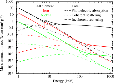
Figure 2: Mass attenuation coefficient of one solar abundance. The dashed-dotted, dotted, dashed curves are the photoelectric absorption, the coherent and incoherent scatterings, respectively. Solid line is the total of them. Black lines represent the mass attenuation coefficient of the all element, while red and green lines show fractional ones of iron and nickel, respectively.

In the coherent scattering, the scattered X-ray does not lose its energy and the differential cross section can be represented as

$$\frac{{\rm d}\sigma_{\rm coh}}{{\rm d}\Omega}=\frac{r_{\rm e}^{2}}{2}(1-\cos^{2}{\theta})F_{m}^{2}(x,Z)=\frac{{\rm d}\sigma_{\rm TM}}{{\rm d}\Omega}F_{m}^{2}(x,Z),$$ (2)

where $r_{\rm e}$ is the classical electron radius, $\theta$ is a scattering angle, $\sigma_{\rm TM}$ is the Thomson cross section and $F_{m}(x,Z)$ is an atomic form factor as a function of an atomic number $Z$ and a momentum transfer

$$x=\frac{\sin{(\theta/2)}}{\lambda},$$ (3)

where $\lambda$ is the wavelength of the incident X-ray in angstrom. We adopted $F_{m}(x,Z)$ evaluated by Hubbell et al. (1975).

By contrast, in the incoherent scattering, the incident X-ray gives energy to an electron and loses a part of its energy. The transferred energy is used for ionization, and hence is larger than the binding energy of the interacting electron. Moreover, the energy of the scattered photon shifts from that scattered by a free electron at rest because of the Doppler effect due to electron orbital motion. A double differential cross section is used for the incoherent scattering and can be represented by Ribberfors & Berggren (1982) as

$$\frac{{\rm d^{2}}\sigma_{\rm incoh}}{{\rm d}E{\rm d}\Omega}=\frac{r_{\rm e}^{2}}{2}\frac{Em_{\rm e}c}{E_{0}cq}\left[1+\left(\frac{p_{\rm z}}{m_{\rm e}c}\right)^{2}\right]^{-1/2}XJ(p_{\rm z})$$ (4)

with the impulse approximation, where $E_{0}$ and $E$ are energies of incident and scattered photon, respectively, $m_{\rm e}$ is the electron mass, $c$ is the velocity of light and $q$ is the modulus of the momentum transfer vector, ${\boldsymbol{q}}={\boldsymbol{k}_{0}}-{\boldsymbol{k}}$, where ${\boldsymbol{k}_{0}}$ and ${\boldsymbol{k}}$ are momenta of incident and scattered photons, respectively. $p_{\rm z}$ is the projection of the initial momentum ${\boldsymbol{p}}$ of the electron on the direction of the scattering vector ${\boldsymbol{k}}-{\boldsymbol{k}_{0}}=-{\boldsymbol{q}}$, that is,

$$p_{\rm z}\equiv-\frac{{\boldsymbol{p}}\cdot{\boldsymbol{q}}}{q}=\frac{E_{0}E(1-\cos{\theta})-m_{\rm e}c^{2}(E_{0}-E)}{c^{2}q}$$ (5)

or

$$\frac{p_{\rm z}}{m_{\rm e}c}=\frac{E_{0}(E-E_{\rm C})}{E_{\rm C}cq},$$ (6)

where

$$E_{\rm C}\equiv\frac{m_{\rm e}c^{2}E_{0}}{m_{\rm e}c^{2}+E_{0}(1-\cos{\theta})}$$ (7)

is the energy of a photon scattered by a free electron at rest (Compton scattering). $X$ in equation 4 is defined as

$$X\equiv\frac{R}{R^{\prime}}+\frac{R^{\prime}}{R}+2\left(\frac{1}{R}-\frac{1}{R^{\prime}}\right)+\left(\frac{1}{R}-\frac{1}{R^{\prime}}\right)^{2},$$ (8)

with

$$R=\frac{E}{m_{e}c^{2}}\left\{\left[1+\left(\frac{p_{\rm z}}{m_{\rm e}c}\right)^{2}\right]^{1/2}+\frac{E_{0}-E\cos{\theta}}{cq}\frac{p_{\rm z}}{m_{e}c}\right\},$$ (9)

and

$$R^{\prime}=R-\frac{E_{0}E}{m_{\rm e}^{2}c^{4}}(1-\cos{\theta})=R-\frac{E}{m_{\rm e}c^{2}}\left(\frac{E_{0}}{E_{\rm C}}-1\right)$$ (10)

$J(p_{\rm z})$ in equation 4 is the Compton profile,

$$J(p_{\rm z})\equiv\int\!\!\!\int\rho({\boldsymbol{p}}){\rm d}p_{\rm x}{\rm d}p_{\rm y},$$ (11)

where $\rho({\boldsymbol{p}})$ is the electron momentum distribution, which can be determined by the state wave function.

We follow a method described by D.Brusa et al. (1996) to reproduce the incoherent scattering. They set $p_{\rm z}/m_{\rm e}c=0$ and $E=E_{\rm C}$ in equation 9 and 10 because $|p_{\rm z}|\sim 0$ is most probable and, therefore, equation 8 reduces to the Klein-Nishina $X$-factor,

$$X_{\rm KN}=\frac{E_{\rm C}}{E_{0}}+\frac{E_{0}}{E_{\rm C}}-\sin^{2}{\theta}.$$ (12)

Moreover, they reproduced the one-electron Compton profiles in the $i$-th shell, $J_{i}(p_{\rm z})$ by an analytical function and obtained $J(p_{\rm z})$ by summing up the one-electron Compton profiles with number of electrons in the $i$-th shell ($Z_{i}$),

$$J(p_{\rm z})=\sum_{i}Z_{i}J_{i}(p_{\rm z}).$$ (13)

Figure 3 shows the averaged differential cross sections of the Compton, coherent and incoherent scatterings at 6.4 keV and 50 keV. The scattering material is of one solar abundance. Each differential cross section in this figure is normalized by its total cross section, which is each differential cross section integrated over the 4$\pi$ solid angle. The incident X-ray is injected from the direction of 180^∘ and collides with the electron at the center. In the coherent scattering, the differential cross section is larger for forward (to 0^∘) scattering than backward (to 180^∘) scattering which becomes more conspicuous for higher energy incident X-rays. Below about 1 keV, it almost converges to that of the Thomson scattering. In contrast, in the incoherent scattering, the differential cross section is larger for backward scattering for lower energy incident X-rays. For a higher energy incident X-ray, it converges to that of the Compton scattering except for the forward scattering. The differential cross section of the incoherent scattering must drop for the forward scattering at any energy of the incident X-ray although the range of the scattering angle within which the forward scattering is reduced, where the coherent scattering is dominant.

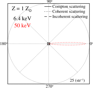
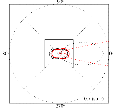
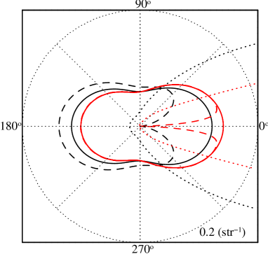
Figure 3: Differential cross sections for an incident X-ray of 6.4 keV (black) and 50 keV (red) scattered off by one solar abundance material. Solid, dotted and dashed lines show the differential cross sections of Compton scattering of a free electron at rest (Klein-Nishina), coherent scattering and incoherent scattering by bound electrons, respectively. These differential cross sections are normalized so that each total cross section becomes unity. In the top panel, the radius of the dotted circle is 25 str^-1. The middle panel is a blowup of the central square in the top panel. The bottom panel is again a blowup of the central square in the middle panel. The radii of the dotted circles are 0.7 and 0.2 str^-1

In this work, re-emission of iron K$\alpha_{1}$ and $\alpha_{2}$ (6.404 and 6.391 keV, respectively), iron K$\beta$ (7.058 keV), nickel K$\alpha_{1}$ and $\alpha_{2}$ (7.478 and 7.461 keV, respectively) and nickel K$\beta$ (8.265 keV) are considered. The photoelectric absorption by iron in a higher energy than its K-edge (7.112 keV) can be undertaken by the K-shell electrons. The K-shell absorption of iron occupies a fraction of 0.876 of the total photoelectric absorption cross section (Storm & Israel, 1970). The fluorescence yield of the iron K-shell is 0.34 and the line relative intensity of K$\alpha_{1}$, $\alpha_{2}$ and K$\beta$ is known to be 100:50:17. Note that the fraction of the K-shell electron absorption to the total photoelectric absorption is assumed to be energy independent although it slightly varies with incident X-ray energy. For Ni, the energy of K-edge is 8.333 keV, the fluorescence yield is 0.38, absorbing faction of K-shell is 0.872 and K$\alpha_{1}$, $\alpha_{2}$ and K$\beta$ line ratio is 100:51:17.

We note that the general relativistic effect is not considered in this work. The energies of the fluorescent lines can be shifted to lower direction by a few eV with the massive WD because these lines are emitted from the surface of the WD where the gravitational redshift is not negligible. The general relativistic effect may work for thermal emission lines as well. We will consider them as well as Doppler effect associated with the plasma flow in the PSAC to apply our model to high energy resolution X-ray data in the future.

3 Results of point source

In this section, results of the Monte Carlo simulation with the point source of a power-law spectrum are summarized.

3.1 Reflected X-ray image

Figures 4 and 5 are reflected X-ray images formed by a point source emitting the power-law spectrum of ${\it\Gamma}=2.0$ from $h$ = 0.0001 and 1 $R_{\rm WD}$, respectively.

In the case of $h$ = 0.0001 (figure 4), the curvature of the WD surface in the reflecting area is negligible and the reflecting surface can be approximated as an infinite plane. Because $h$ is sufficiently small compared with the WD radius, the reflecting area on the WD is sufficiently narrow. Most reflection occurs in a circle of the radius of 0.001 $R_{\rm WD}$ (see figure 4). For a larger viewing angle, the image is elongated along the reflected direction. This feature is caused by the anisotropy of the differential cross sections of the scattering as previously reported by George & Fabian (1991). Incident X-rays are more easily scattered to a direction close to the incident direction. The incident direction and reflecting direction is closer when reflection position is more distant from the position right down the point source. Consequently when the viewing angle is larger, the image extends more in the reflecting direction.

In the case of $h=R_{\rm WD}$ in figure 5, the WD curvature is not negligible. Because of the curvature, X-rays are reflected to the viewing angle over 90 deg and occultation by the WD limb occurs unlike the case of $h$ = 0.0001 $R_{\rm WD}$. Moreover, the image extension appearing in the large viewing angle of the $h$ = 0.0001 $R_{\rm WD}$ case does not appear because the curvature radius of the reflector (WD) comparable to the height of the X-ray source precludes the incident direction and reflected direction from getting closer, unlike the case of $h=0.0001\,R_{\rm WD}$.

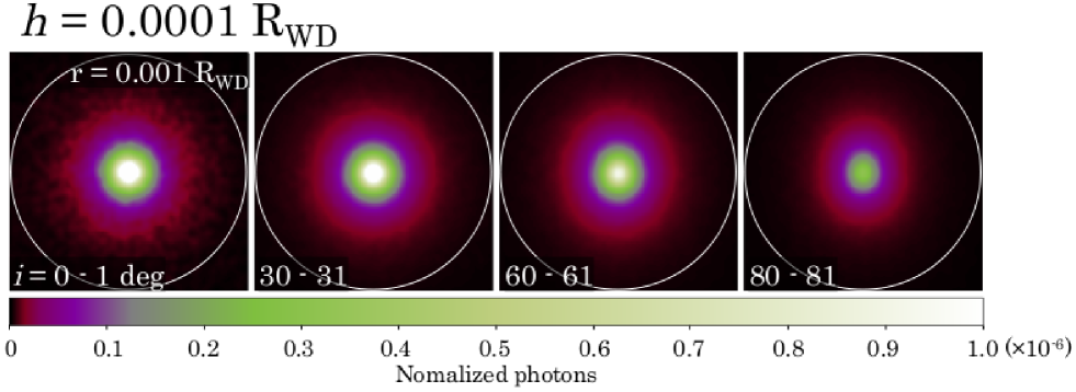
Figure 4: Reflection X-ray images with a point source located at 0.0001 $R_{\rm WD}$ above the WD surface. Incident X-rays have a power-law spectrum with ${\it\Gamma}$ = 2.0 in the band 1–500 keV. A white circle in each panel is centered on the position on the WD surface right down the point source with a radius of 0.001 $R_{\rm WD}$. The scattering direction is contained in a plane defined by an in-plane vertical line and a normal to the page. Range of viewing angle ($i$, see Fig. 1) is 0–1, 30–31, 60–61and 80–81 degrees from left to right. These images are normalized with generated photon number and smoothed by Gaussian function with $\sigma$ of 3$\times$10^-5 $R_{\rm WD}$. Note that the fluctuation appeared in the viewing angle of $i=0-1$ deg is caused by Poisson noise because the solid angle is extremely small compared to the other viewing angle.

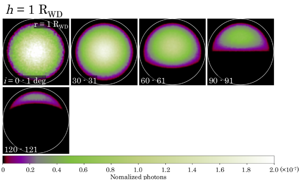
Figure 5: Same as Figure 4, but a point X-ray source is located at 1 $R_{\rm WD}$ above the WD, where 1 $R_{\rm WD}$ is the radius of the WD. Range of reflecting angle ($i$) is 0–1, 30–31, 60–61, 90–91 and 120–121 degrees from left to right and top to bottom. These images are normalized by generated photon number and smoothed by Gaussian function with $\sigma$ of 3$\times$10^-2 $R_{\rm WD}$.

3.2 Spectrum

Spectral structures of the reflection manifest themselves over the intrinsic spectrum in the following two energy domains. One is the fluorescent emission line in the band of 6–9 keV, and the other is the Compton hump formed around 10-50 keV by a sequence of energy loss by the incoherent scattering and photoelectric absorption (figure 2). Figure 6 shows the reflection spectra with ${\it\Gamma}=2.0$ for intrinsic power-law spectrum, $h$ = 0.0001 and 1 $R_{\rm WD}$ and, $i$ = 0–10, 30–40 and 80–90 deg. This figure clearly shows the fluorescent lines, their Compton shoulder and the Compton hump. The Compton shoulder is formed by the incoherent scattering of the fluorescent photons. The reflection containing all of the spectral features mentioned above is reduced as $h$ increases because a solid angle of the WD surface viewed from the point source becomes small. The reflection becomes less intense for larger $i$ because a longer optical path is needed to escape out from the WD. The details of the line emissions and the Compton hump are described below.

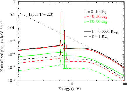
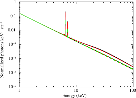
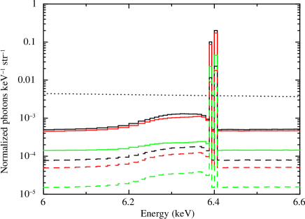
Figure 6: Reflected X-ray spectra from a cool and spherical WD. The spectrum of the irradiating point source is a power law with ${\it\Gamma}$ = 2.0 (dotted line). The height of the point source is assumed at $h$ = 0.0001 $R_{\rm WD}$ (solid line) and 1 $R_{\rm WD}$ (dashed line). The viewing angle $i$ is 0–10 (black), 40–50 (red) and 80–90 deg (green). The middle panel shows the total spectra of the intrinsic and reflected emission components. The bottom panel is magnification of part of the iron K$\alpha_{1,2}$ lines of the top panel. Note that horizontal axis of the bottom panel is linear scale unlike the other panels.

3.2.1 Iron K$\alpha_{1,2}$ lines and their Compton shoulders

The bottom panel of figure 6 is magnification of the reflected X-ray spectra in 6–8.5 keV where the iron K$\alpha_{1,2}$ lines appear with their Compton shoulder. A valley between the fluorescent iron K$\alpha_{1,2}$ lines and their Compton shoulder is due to the small cross section of incoherent forward scattering (see figure 3). Moreover, shape of the Compton shoulder is not double peak, unlike the case of the Compton scattering by free electrons at rest, because the double peak is blurred by the Doppler effect caused by the momentum of the bound electrons. We note that the lines at the original energies contain fluorescent photons directly arriving at the observer and those undergoing the coherent scattering(s). We, however, do not discriminate them and just call their original name such as fluorescent iron K$\alpha_{1}$ line.

Hereafter, we concentrate on the iron K$\alpha_{1,2}$ lines. We assume that the abundance is 1 $Z_{\odot}$ unless otherwise noted. We define an energy centroid of the iron K$\alpha_{1,2}$ fluorescent lines with their Compton shoulder as

$$E_{\rm cen}=\frac{\int^{E_{1}}_{E_{0}}{\rm d}EE\left\{I_{\rm ref}(E)-I_{\rm ref\mathchar 45\relax cont}(E)\right\}}{\int^{E_{1}}_{E_{0}}{\rm d}E\left\{I_{\rm ref}(E)-I_{\rm ref\mathchar 45\relax cont}(E)\right\}},$$ (14)

where $I_{\rm ref}(E)$ and $I_{\rm ref\mathchar 45\relax cont}(E)$ are the intensity of the reflection in total and that of the continuum (excluding fluorescent photons), respectively, at an energy of $E$ in unit of keV. We adopted (6.100, 6.405) as the set of ($E_{0}$, $E_{1}$). We remark that $I_{\rm ref}(E)-I_{\rm ref\mathchar 45\relax cont}(E)$ is the spectrum of the iron K$\alpha$ lines and their reprocessed emission.

Figure 7 shows the energy centroid slightly increases by $\sim$ 10 eV as $i$ increases. This is because the intensity ratio of the Compton shoulders to that of the original lines (see below) is smaller with increasing $i$. We note that the difference of the centroid from 6.4 keV is no more than 20 eV.

Figure 7: Relation between the viewing angle $i$ and the energy centroid averaged over the fluorescent iron K$\alpha_{1,2}$ lines and their Compton shoulders. Solid and dashed lines assume $h$ = 0.0001 and 1 $R_{\rm WD}$ for the irradiating point source. Photon index of the source is assumed to be ${\it\Gamma}$ = 2.0.

We define a line equivalent width (EW) as

$$EW=\int^{E_{1}}_{E_{0}}{\rm d}E\frac{I_{\rm ref}(E)-I_{\rm ref\mathchar 45\relax cont}(E)}{I_{\rm pl}(E_{\rm cen})+I_{\rm ref\mathchar 45\relax cont}(E_{\rm cen})}$$ (15)

where $I_{\rm pl}(E)$ is intensity of the intrinsic power law at a energy of $E$ and $E_{\rm cen}$ is the energy centroid of the line in question. In equation 15, $I_{\rm ref\mathchar 45\relax cont}(E)$ is subtracted from $I_{\rm ref}(E)$ to extract the line photons only in the numerator, and add the reflection continuum to the power law continuum to calculate total continuum in the denominator. Sets of ($E_{0}$, $E_{1}$) for K$\alpha_{1}$ and K$\alpha_{2}$ are (6.403, 6.405) and (6.390, 6.392), respectively, and for the total of the K$\alpha_{1,2}$ lines with their Compton shoulder is (6.100, 6.405). $E_{\rm cen}$ for the K$\alpha_{1,2}$ lines are their nominal energies (see §2.2) and that for total of the K$\alpha_{1,2}$ lines with their Compton shoulder is shown in figure 7.

Figure 8 clearly exhibits that monotonic decrease of the EWs against increase of the viewing angle $i$ irrespective of $h$. This is because the optical path is longer in larger $i$, which makes the line photon difficult to escape from the WD. The EW of the K$\alpha_{1,2}$ lines in the case of the $h=0.0001\,R_{\rm WD}$ is consistent with the calculation of George & Fabian (1991) although the authors assumed the Compton scattering with free and stationary electrons which are distributed on a flat disc with a radius of 100 times larger than a point source height. In higher $h,$ the solid angle of the WD viewed from the point source becomes smaller and therefore, the EW becomes smaller. Moreover, significant EW appears in the viewing angle larger than 90 deg in higher $h$ because of the spherical shape of the WD although the EW is small ($<$ 10 eV). We note that EW ratio of the K$\alpha_{1,2}$ is 2:1 with any $i$ and $h$ according to their relative intensity (§2.2).

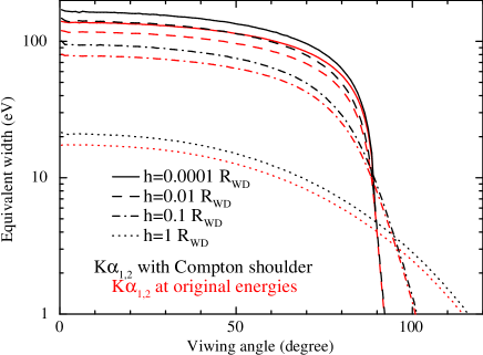
Figure 8: Relation between the viewing angle $i$ and the EWs of the complex of the fluorescent iron K$\alpha$ line. Solid, dashed, dashed-dotted and dotted lines are the cases of $h$ = 0.0001, 0.01, 0.1 and 1 $R_{\rm WD}$ for the point source, respectively. The black and red lines show the EW of sum of the iron K$\alpha_{1,2}$ lines with and without their Compton shoulder, respectively. Photon index of the source is assumed to be ${\it\Gamma}$ = 2.0.

The EW ratio of the Compton shoulder to sum of the fluorescent iron K$\alpha_{1,2}$ lines decreases as $i$ increases as shown in figure 9. The EW of the Compton shoulder is obtained by equations 14 and 15 using ($E_{0}$, $E_{1}$) of (6.100, 6.390). This drop of the intensity ratio with increasing $i$ is caused by the following two effects. One is the fact that a fluorescent line photon generated deeper in the WD can experience a larger number of scatterings before escaping from the WD surface. This means that a line spectrum from a deeper layer possesses a more prominent Compton shoulder. The other is that in larger $i$, only photon whose last interaction occurs at a shallower layer can escape out from the WD surface because the optical path to escape from the WD increases by 1/$\sin(90-i)$. One can observe a reflection spectrum from a shallower layer of the WD in a larger $i$ configuration, which reduces the EW of the Compton shoulder relative to the seed iron K$\alpha_{1,2}$ lines.

Figure 9: EW ratio of the Compton shoulder of the fluorescent iron K$\alpha_{1,2}$ lines to the sum of the EWs of iron K$\alpha_{1,2}$ lines at respective original energies. Solid and dashed lines are the cases of $h$ = 0.0001 and 1 $R_{\rm WD}$ for the irradiating point source.

Figure 10 shows ratio of the EW calculated for various intrinsic spectra to that for the spectrum with ${\it\Gamma}=2.0$. The EW ratio increases with decreasing ${\it\Gamma}$. This is because the number of photons with the energy higher than the absorption edge (7.11 keV) increases when ${\it\Gamma}$ decreases. Note that the EW ratio is insensitive to $h$, especially in high ${\it\Gamma}$. The larger $i$ suppresses the number of the escaping photons from deeper layer, as explained above. A smaller ${\it\Gamma}$ spectrum contains a larger number of more energetic photons that can produce the iron K$\alpha_{1,2}$ lines in a deeper layer of the WD. Such iron lines, however, do not escape from the WD in a higher $i$ case, because of a longer absorption path within the WD. Consequently, larger $i$ reduces the difference of the EW caused by ${\it\Gamma}$.

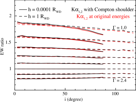
Figure 10: EW ratio of the sum of the fluorescent iron K$\alpha_{1,2}$ lines of various ${\it\Gamma}$ to that of ${\it\Gamma}=2.0$ (see figure 8) versus the viewing angle $i$. Solid and dashed lines are cases of $h$ = 0.0001 and 1 R_WD, respectively. Black and red lines contain the iron K$\alpha_{1,2}$ lines with and without their Compton shoulder, respectively. These four cases are calculated for ${\it\Gamma}$ of 1.0 to 2.4 with an interval of 0.2.

3.2.2 Compton hump

Compton hump varies with $i$ and $h$ in its intensity and shape (see figure 6). Figure 11 shows intensity ratios of the reflection to the intrinsic power law versus the viewing angle in 35–50 keV and 10–100 keV for various $h$. The relation between the ratio and $i$ is similar to the relation between the EW and $i$ (figure 8).

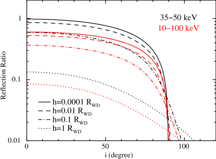
Figure 11: Ratio of the X-ray reflection to the intrinsic component in the viewing angle $i$. Black and red lines calculated in energy bands of 35–50 keV and 10–100 keV, respectively. Solid, dashed, dashed-dotted and dotted lines are cases of $h$ of 0.0001, 0.01, 0.1 and 1 $R_{\rm WD}$. ${\it\Gamma}$ = 2.0 is assumed.

The top panel of figure 6 shows that the spectrum scattered off in 0–10 deg has a well defined Compton hump, whose peak is less prominent in larger $i$, especially in 80–90 deg. As previously mentioned, the larger $i$ suppresses the number of interactions (incoherent scattering is dominant above 10 keV, see figure 2), therefore, the less number of interactions makes the shape of Compton hump close to that of the intrinsic spectrum.

Unlike the emission line, the Compton hump can hardly be separated from the intrinsic continuum in actual data. Nevertheless, we should evaluate the shape of the Compton hump with the total spectrum which includes the intrinsic power law and the reflection. Figure 12 shows ratios of intensity of the total spectrum in 10–35 keV and 50–100 keV to 35–50 keV. The ratios drop toward a smaller $i$, which shows that the reflection component in 35–50 keV is stronger than those in the other bands, especially in small $i$. The ratios with $i>90$ deg are almost constant because they are determined by the intrinsic power law.

These intensity ratios depend on ${\it\Gamma}$ as shown in figure 13. We note that the difference in ${\it\Gamma}$ appears mainly in offsets of the intensity ratios with only small dependence on $i$, which is caused by the nature of the reflection whose spectral shape approaches the intrinsic power law in larger $i$ because the number of interactions is suppressed.

Figure 12: Ratio of intensity of the total (intrinsic + reflected) spectrum in 10–35 keV (top) and 50–100 keV (bottom) to that in 35–50 keV versus the viewing angle $i$. Solid, dashed, dashed-dotted and dotted lines are cases of $h$ of 0.0001, 0.01, 0.1 and 1 $R_{\rm WD}$. ${\it\Gamma}$ = 2.0 is assumed.

Figure 13: Ratio of intensity in 10–35 keV (top) and 50–100 keV (bottom) of various ${\it\Gamma}$ to that in 35–50 keV of $\Gamma=2.0$ (see Figure 11) as a function of the viewing angle $i$. Solid and dashed lines are cases of $h$ of 0.0001 and 1 $R_{\rm WD}$. Calculation is made for these two cases at ${\it\Gamma}$ of 1.0 to 2.4 with an interval of 0.2 are used to the two-line groups from bottom to top in the top panel and from top to bottom in the bottom panel.

3.2.3 Influence of abundance

The fluorescent iron K$\alpha_{1,2}$ lines, their Compton shoulder and Compton hump are influenced by the abundance. Figure 14 shows plots of the line EWs versus the abundance with various viewing angle ($i$) and heights of the source ($h$). The EWs initially increase with the abundance, but peaks out at certain abundances in all cases, as reported in George & Fabian (1991).

When the abundances of all elements are simultaneously increased from zero ((a) and (b) of figure 14), the probability of the absorption of all elements including iron is enhanced relative to the scattering by degrees. Consequently, the EW increases as the abundances increase. In the higher abundances where the scattering becomes negligible, the EW peaks out around 1 and 0.2 solar abundance for h = 0.0001 and 1 $R_{\rm WD}$, respectively, because the iron abundance relative to the others is constant. By contrast, their Compton shoulders decrease in the dashed green line in panel (a) of figure 14 because the scattering is suppressed. The decrease of the Compton shoulder counteracts the increase of the EW of the iron K$\alpha_{1,2}$ lines.

When only the iron abundance is varied and the other abundances are fixed at 1 solar abundance ((c) and (d) of figure 14), the EWs are proportional to the iron abundance when the iron abundance is lower than 1 and 0.5 solar abundance for $h=0.0001$ and 1 $R_{\rm WD}$, respectively. With larger iron abundance, the increase of the EW becomes gentle because the total cross section is dominated by photoelectric absorption of iron and the probability of absorption by iron asymptotically becomes constant. The EW of Compton shoulders also increase as the iron abundance increases (dashed green line in panel (c) of figure 14) because the scattering is mainly caused by lighter elements than iron and is not suppressed by the low iron abundance. With larger iron abundance than the range of figure 14), the EW of the Compton shoulders becomes constant as the EWs of the K$\alpha_{1,2}$ lines, because the cross sections of the scatterings are also determined by iron (George & Fabian, 1991).

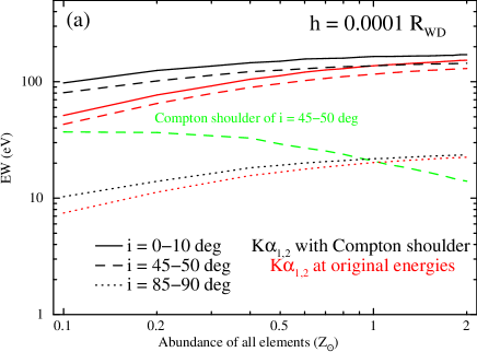
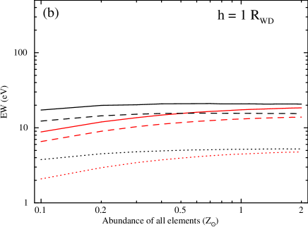
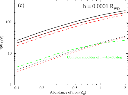
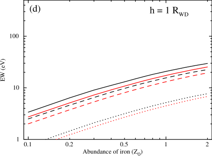
Figure 14: Relations between abundance and the total EW of the fluorescent iron K$\alpha_{1,2}$ lines. Abundances of all elements are varied at the common rate relative to the solar composition in the top two panels ((a), (b)). In the bottom panels ((c), (d)), only iron abundance is varied and the others are fixed at one solar abundance. $h$ = 0.0001 $R_{\rm WD}$ and 1 $R_{\rm WD}$ cases are shown in the left ((a), (c)) and the right ((b), (d)) panels, respectively. Solid, dashed and dotted lines are cases of $i$ = 5, 45 and 85 deg, respectively. The total EW of the fluorescent iron K$\alpha_{1,2}$ lines and their corresponding Compton shoulder is shown by black lines and that of the fluorescent iron K$\alpha_{1,2}$ lines is shown by red lines. Green dashed line presents the EW of the Compton shoulder in the panels of $h=0.0001\,R_{\rm WD}$ ((a), (c)) with $i$ = 45–50 deg.

The Compton hump depends on the abundance as well as the fluorescent iron K$\alpha_{1,2}$ lines. Figure 15 shows ratios of intensity in 10–35 keV and 50–100 keV to that in 35–50 keV as functions of the abundance with various $i$ and $h$. This figure indicates that the intensity in 10–35 keV decreases and by contrast, that in 50–100 keV increases against that in 35–50 keV in any cases, which means that cut-off energy of the Compton hump increases as the abundance increases. The heavier photoelectric absorption caused by the higher abundance results in a larger absorption optical depth at any given energy, and, as a result, increases the cut-off energy

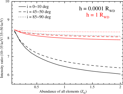
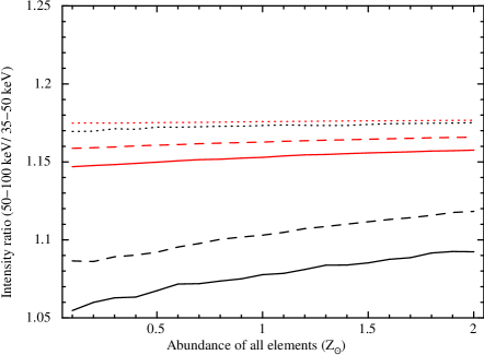
Figure 15: Relations between abundance and the ratio of intensities in 10-35 keV (left) and 50-100 keV (right) to that in 35-50 keV. Abundances of all elements are varied at the common rate relative to the solar composition. $h$ = 0.0001 $R_{\rm WD}$ and 1 $R_{\rm WD}$ are shown with black and red, respectively. Solid, dashed and dotted lines are the cases of $i$ = 5, 45 and 85 deg, respectively.

4 PSAC source

In this section, we present results of the simulation using the PSAC source introduced in §2.1. The shape of reflection spectrum depends on the WD mass, the specific accretion rate, the abundance and the viewing angle. The results with the PSAC source are more complex than those with a point source of a power-law spectrum (§ 3). However, the reflection spectrum with the PSAC source can be basically represented by summation of the point sources.

4.1 Spectrum

4.1.1 dependence on the viewing angle

Figure 16 shows spectra of the intrinsic thermal plasma, the reflection and the total of them with $i$= 0–10 deg and 80–90 deg, $M_{\rm WD}$ = 0.7 $M_{\odot}$ and $a$ = 1 g cm^-2 s^-1. The reflection decreases as $i$ increases and the Compton shoulder shape of the fluorescent lines varies in common with that of the point source of the power-law spectrum. The reflection spectrum has Compton shoulders of He-like and H-like iron K$\alpha$ emission lines at around a few hundred eV down of their nominal line energies (see bottom of figure 16). The scattered line profile is flatter in larger $i$. If we confine ourselves to consider a low enough PSAC ($h\ll R_{\rm WD}$) and a single scattering as shown in figure 17, around $i$ $\sim 0$ deg, the scattering angle is limited in 90–180 deg. On the other hand, around $i$ $\sim 90$ deg, the scattering angle is permitted to be 0–180 deg. Consequently, the scattered line profile becomes flatter and wider as $i$ increases. The fluorescent lines do not change by this effect because they are originated within the WD unlike the intrinsic lines.

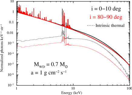
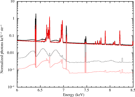
Figure 16: PSAC spectra with the WD mass of 0.7 $M_{\odot}$, the specific accretion rate of 1 g cm^-2 s^-1 and $i$ of 0-10 (black) and 80-90 deg (red). Solid, thin solid and dotted lines are the total, the reflection and the intrinsic thermal plasma components, respectively. Bottom panel is a blowup in 6–8.5 keV.

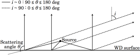
Figure 17: Scattering paths of photons from a source above the WD. When the reemitted photon is reflected to $i\sim$ 0 deg (solid line), the scattering angle is between 90 and 180 deg. By contrast, when the reflection angle $i\sim$90 deg (dashed line), the scattering can occur at any angle between 0 and 180 deg.

Although it is weak, the reflection with the PSAC source may appear in the domain $i>$ 90 deg as shown by red in figure 18 (where WD of 1.2 $M_{\odot}$ and $a$ = 0.01 g cm^-2 s^-1 are adopted and the resultant PSAC height is $\sim$ 33% of the WD radius) because of the finite height of the PSAC source. In this case, only photons grazing the WD surface and then getting scattered forward appear. The coherent scattering is dominant in this situation (see figure 3). Consequently, the energies of the scattered lines nearly agree with those of the intrinsic lines. Note that the intrinsic thermal spectrum which can be seen from the observer in the case of $i>90$ deg is harder than that of $i<90$ deg because a lower PSAC part consisting of a low-temperature and high-density plasma is occulted by the WD and only the hotter higher part is visible.

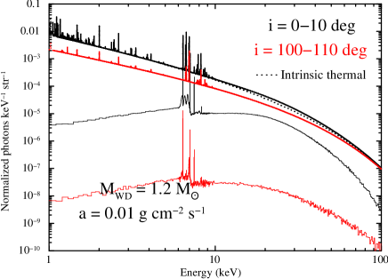
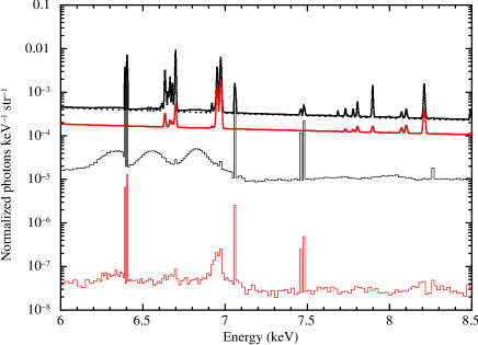
Figure 18: PSAC spectra with the WD mass of 1.2 $M_{\odot}$, the specific accretion rate of 0.01 g cm^-2 s^-1, and $i$ of 0–10 (black) and 100–110 deg (red). Solid, thin solid and dotted lines are the total, the reflection and the intrinsic thermal plasma components, respectively. Bottom panel is a blowup in 6–8.5 keV.

4.1.2 Dependence on the WD mass

Figure 19 shows the PSAC X-ray spectra with the WD masses of 0.4 $M_{\odot}$ and 1.2 $M_{\odot}$, the specific accretion rate of $a$ = 1 g cm^-2 s^-1 and the viewing angle of $i$ = 40–50 deg. The more massive WD makes a harder intrinsic thermal spectrum because of its deeper gravitational potential. The harder intrinsic spectrum enhances the the fluorescent lines and the Compton hump as shown in §3.2. By contrast, the PSAC is taller relative to the WD radius for the more massive WD because the more massive WD has a smaller radius and a taller PSAC due to longer cooling time (e.g. Hayashi & Ishida 2014a). The taller PSAC preferentially reduces the contribution of its higher part to the reflection. Consequently, the WD mass intricately influences the reflection. For example, the EW of the fluorescent iron K$\alpha_{1,2}$ lines is not a monotonically increasing function of the WD mass in a certain domain of the specific accretion rate as described later (§4.2).

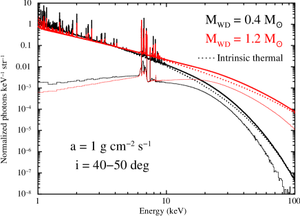
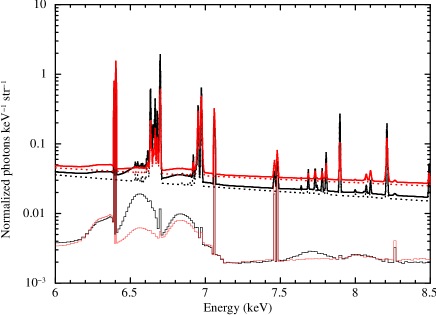
Figure 19: PSAC spectra with the WD mass of 0.4 $M_{\odot}$ (black) and 1.2 $M_{\odot}$ (red), the specific accretion rate of 1 g cm^-2 s^-1 and $i$ of 40-50 deg. Solid, thin solid and dotted lines are the total, the reflection and the intrinsic thermal plasma components, respectively. Bottom panel is a blowup in 6–8.5 keV.

4.1.3 Dependence on the specific accretion rate

The specific accretion rate also influences the intrinsic thermal and the reflection spectra. Figure 20 shows the X-ray spectra with the specific accretion rates of $a$ = 100 g cm^-2 s^-1 and 0.01 g cm^-2 s^-1, the WD mass of 0.7 $M_{\odot}$ and the viewing angle of $i$ = 40–50 deg. The smaller specific accretion rate increases the cooling time and lengthens the PSAC. With the taller PSAC, released gravitational energy at the shock is less which makes the PSAC cooler and the intrinsic thermal spectrum softer. The taller and cooler PSAC reduces the reflection. Consequently, the influence of the specific accretion rate on the reflection is simpler than that of the WD mass. The EW of the fluorescent iron K$\alpha_{1,2}$ lines monotonically increases irrespective of the WD mass as the specific accretion rate increases (§4.2).

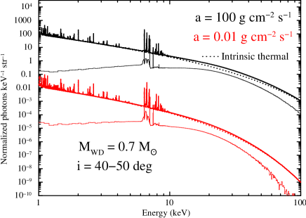
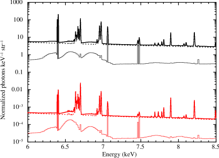
Figure 20: PSAC spectra with the WD mass of 0.7 $M_{\odot}$, the specific accretion rate of 100  g cm^-2 s (black) and 0.01  g cm^-2 s^-1 (red) and $i$ of 40–50 deg. Solid, thin solid and dotted lines are the total, the reflection and the intrinsic thermal plasma components, respectively. Bottom panel is a blowup in 6–8.5 keV.

4.2 Sum of the EWs of fluorescent ion K$\alpha_{1,2}$ lines

Figure 21 shows the EWs of the sum of the fluorescent iron K$\alpha_{1,2}$ lines, and those with their Compton shoulders as a function of the specific accretion rate. In this figure, the cases of the WD masses of $M_{\rm WD}$ = 0.4, 0.7 and 1.2 $M_{\odot}$ and the viewing angles of $i$ = 0–10, 45–50 deg and 85–90 deg are shown.

The EWs monotonically increase with the specific accretion rate for any WD mass because the PSAC shortens and the its temperature rises (see Hayashi & Ishida 2014a). However, they become almost constant at the highest end of the specific accretion rate in this figure. This is because, in the larger specific accretion rate, the distributions of physical quantities normalized by the PSAC height does not vary, and its height is negligible against the WD radius. Moreover, in the smaller specific accretion rate, the maximum of the electron temperature in the PSAC is hardly affected by the specific accretion rate.

The influence of the WD mass on the reflection is more complex because a more massive WD raises the PSAC temperature and extends the PSAC, which enhances and reduces the reflection, respectively. In fact, the EWs in figure 21 rise and fall as the WD mass increases in the specific accretion rate between 0.01–100 g cm^-2 s^-1. The relations between the EWs and the WD masses also depend on the viewing angle. Irrespective of the specific accretion rate and the WD mass, comparison of the three panels in figure 21 indicates that the EWs decrease with increasing viewing angle.

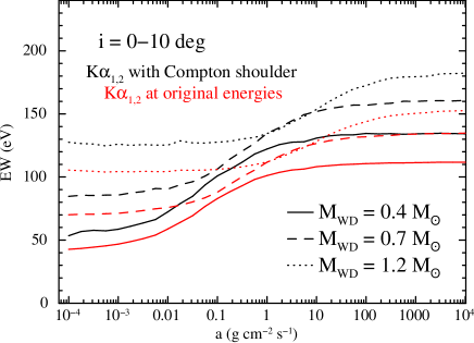
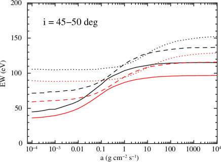
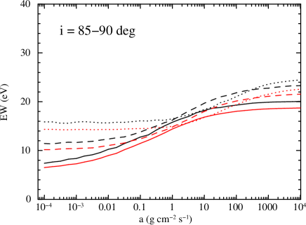
Figure 21: Relations between the specific accretion rate and the sum of the EWs of the fluorescent iron K$\alpha_{1,2}$ lines (red lines), and the total EW of the fluorescent iron K$\alpha_{1,2}$ lines and their Compton shoulders (black lines) with the WD masses of 0.4, 0.7 and 1.2 $M_{\odot}$ (solid, dashed and dotted lines, respectively). $i$ of 0–10, 45–50 and 85–90 deg are assumed in the top, middle and bottom panels, respectively.

4.3 Compton hump

Since the Compton hump is the other important ingredient of the reflection spectrum, it also depends on the WD mass and the specific accretion rate although its variation is somewhat minor compared to that of the intrinsic thermal spectrum. Figure 22 shows the ratio of the continuum intensity in 10–35 keV to that in 35–50 keV with the WD masses of $M_{\rm WD}$ = 0.4 $M_{\odot}$ and 1.2 $M_{\odot}$, and the viewing angles of $i$ = 0–10, 45–50 and 85–90 deg. This figure indicates that the influence of the viewing angle on the intensity ratio is limited. Especially, the intensity ratio of less massive WD (e.g. $M_{\rm WD}$ = 0.4 $M_{\odot}$) hardly depends on the viewing angle. This fact means that the shape of the reflection spectrum (the softness ratio) depends mainly on the intrinsic thermal spectrum (uniquely determined by the specific accretion rate at a given WD mass). On the other hand, in the case of more massive WD (e.g. $M_{\rm WD}$ = 1.2 $M_{\odot}$), the intensity ratio varies with the viewing angle and the reflection spectrum is more sensitive to the viewing angle.

Figure 22: Relations between the specific accretion rate and the ratio of intensity in 10–35 keV to that in 35–50 keV with the WD masses of 0.4 and 1.2 $M_{\odot}$ (top and bottom panels, respectively) and $i$ of 0–10 (solid), 45–50 (dashed) and 85–90 (dotted) deg.

4.4 Spin profile

In general, a reflection X-ray spectrum of the mCVs varies in association with the WD spin phase because the PSAC is not coaligned with the WD spin axis. It has been well known from observations that the photoelectric absorption by the pre-shock accreting matter can bring about spin modulation of the X-ray intensity. However, here, we concentrate on the spin modulations of the reflection and the intrinsic thermal plasma component caused by the occultation.

The spin modulation of a single PSAC is determined by angles of the spin axis from the line of sight ($\alpha$) and from the PSAC ($\beta$) as well as the WD mass, the specific accretion rate and the abundance. The spin modulation also depends on whether the two PSACs can be seen. Figure 23 shows the spin modulations in cases of $M_{\rm WD}=0.7\,M_{\odot}$ and $\alpha$ = 20 deg as common parameters, and specific accretion of $a$ = 1.0 and 0.01 g cm^-2 s^-1, and $\beta$ = 45 and 80 deg. Here, we assume that the upper and possible lower PSACs are separated by 180^∘ on the WD surface.

In the case of $a$ = 1.0 g cm^-2 s^-1 and $\beta=45$ deg, the upper PSAC can always be seen and the possible lower PSAC is invisible in any phase. Consequently, the spin modulation is brought about only by the reflection whose intensity varies sinusoidally with the pulse fraction of about 30% and 10% in the fluorescent iron K$\alpha_{1,2}$ lines and 35–50 keV band, respectively. The intensity in 1–100 keV is almost constant because it is almost determined by the intrinsic thermal component.

When $a$ = 0.01 g cm^-2 s^-1 and the other parameters are common with the previous case, the PSAC becomes taller and the top of the possible lower PSAC is visible except for around phase of 0.5. Since the top of the PSAC is hot ($>$ 10 keV), the thermal component in the 35–50 keV significantly rises around the phase of 0. Consequently, the spin modulation is not sinusoidal. The pulse fraction in the 35-50 keV is about 10% without the lower PSAC and 30% with the lower PSAC. Note, however, that the intensity of the fluorescent iron K$\alpha_{1,2}$ lines are not influenced by the lower PSAC because its base where the lines are emitted is mostly behind the limb of the WD.

When $\beta$ = 80 deg and the other parameters are common with the first case, both the upper PSAC and the possible lower PSAC are seen and occulted in turn. The spin profiles are complex and significantly change with the X-ray energy. The spin profile of the fluorescent iron K$\alpha_{1,2}$ lines has a single-peak profile with 100% amplitude when the lower PSAC does not exist. When the lower PSAC exists, its profile is a double peak. In the 35–50k̇eV band, the single-peak with 50% amplitude profile appears when the lower PSAC is not present. When the lower PSAC is took into account, the spin profile has two flat regions centered at the phases of 0 and 0.5 whose intensities differ by about 30%. The spin profile of the 1–100 keV intensity has a dip around the phase 0 with 70% amplitude if we consider only the upper PSAC. With the upper and the lower PSACs, the spin profile has two peaks which correspond to the phases of switching the two PSACs.

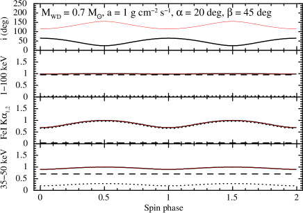
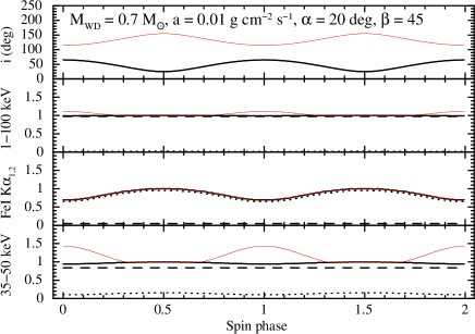
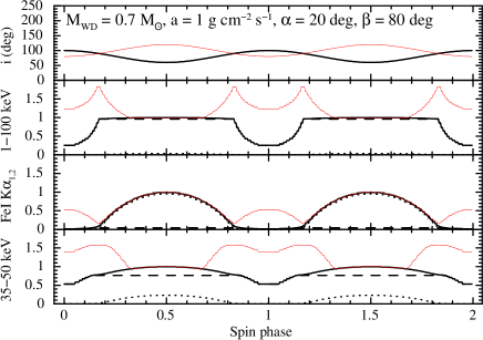
Figure 23: Spin profiles with the WD mass of 0.7 $M_{\odot}$ and the angle of the spin axis from the line of sight ($\alpha$) of 20 deg. Sets of the specific accretion rate (g cm^-2 s ^-1) and the angle of PSAC from the line of sight $\beta$ (deg) are assumed to be 1 and 45 in the top panel, 0.01 and 45 in the middle panel and 1 and 85 in the bottom panel. Top boxes in the individual panels show $i$ of the upper pole (black) and the possible lower pole (red). Bottom three boxes in the individual panels are spin profiles of the intensities in the 1–100 keV band, of the 6.4 line and in the 35–50 keV band toward bottom. Black dotted, dashed and solid lines are the intensities of the reflection, the intrinsic thermal components and sum of them, which are normalized by the maximum of the sum. Red line is the total of the sum of the upper and the possible lower poles and normalized by the common value with black lines (the total of upper pole).

5 Discussion

5.1 Measurement of system parameters

Geometrical parameters such as the viewing angle and the height of the intrinsic X-ray source can be measured with our reflection model. Since the observed spectrum is the sum of the intrinsic PSAC spectrum and its reflection, the reflection model is of essential importance to evaluate the shape of the intrinsic PSAC spectrum, which enhances the measurement accuracy of the parameters of the thermal component such as the WD mass and the specific accretion rate in cooperation with the intrinsic thermal model of the PSAC (e.g. Hayashi & Ishida 2014a).

The EW of the fluorescent iron K$\alpha$ line is significantly different among the IPs. For instance, the EW of EX Hya and TV Col were measured to be 24 eV (Hayashi & Ishida, 2014b) and 170 eV (Ezuka & Ishida, 1999), respectively. The small EW such as that of EX Hya suggests that the system has a light WD, low specific accretion rate, low metal abundance and a large viewing angle (see figure 21). The WD mass and the specific accretion rate of EX Hya were measured in some works, for example : $M_{\rm WD}=0.790\pm 0.026\,M_{\odot}$ (Beuermann & Reinsch, 2008), $M_{\rm WD}=0.4\pm 0.02\,M_{\odot}$ with $a$ fixed at 1 g cm^-2 s^-1 (Yuasa et al., 2010) and $M_{\rm WD}=0.63^{+0.17}_{-0.14}\,M_{\odot}$ and $a$ = 0.049${}^{+0.66}_{-0.04}$ g cm^-2 s^-1 (Hayashi & Ishida, 2014b). All of them need a large viewing angle $i>60$ deg to explain the small EW with the measured iron abundance of 0.57$\pm 0.03$ (Hayashi & Ishida, 2014b). If the line emission from the pre-shock absorption matter contributes to the EW, an even larger viewing angle is required. By contrast, the large EW 170 eV of TV Co implies that the WD should be massive as long as the entire fluorescent K$\alpha_{1,2}$ lines originate from the WD surface. However, there is significant contribution from the pre-shock cold accreting matter to the EW (Ezuka & Ishida, 1999), which makes difficult to put a constraint from the EW on the WD mass. However, since the central energies of the K$\alpha$ lines from the pre-shock accreting matter shift from the values in laboratories according to the radial flow velocity of the flow, they will be resolved from those from the WD surface with a high resolution detector, such as a micro-calorimeter, in the near future.

The Compton hump is another important spectral feature to constrain some system parameters such as the viewing angle and the height of the PSAC, like the fluorescent iron lines, yet it is difficult to resolve it from the observed continuum spectrum because its spectrum spreads widely in energy and somewhat similar to the intrinsic PSAC spectrum. Recent observations of some IPs with the NuSTAR satellite undoubtedly verified existence of the Compton hump (Mukai et al., 2015). However, it is difficult to segregate the Compton hump from the intrinsic PSAC thermal spectrum with enough accuracy to evaluate the system parameters. The Compton hump is useful to constrain the parameters only if its accurate spectral model like ours presented in this paper is applied to the observed spectrum in combination with the fluorescent iron K$\alpha$ line. Application of the reflection model with the intrinsic PSAC thermal model (Hayashi & Ishida, 2014a) to observational data will be presented in a subsequent paper.

5.2 Interpretation of the red wing of the fluorescent iron K$\alpha$ line

The iron fluorescent K$\alpha$ line has a red wing in some IPs. For GK Per in outburst, the red wing extending to 6.33 keV was observed by High-Energy Transmission Grating (HETG) onboard the Chandra satellite (Hellier & Mukai, 2004). In addition, the Suzaku observation of V1223 Sgr with CCD cameras (X-ray Imaging Spectrometer: XIS) reveals that the energy centroid of the fluorescent iron K$\alpha$ line synchronously modulates with the WD spin (Hayashi et al., 2011). The energy centroid is shifted from the rest frame value 6.40 keV and reaches the minimum of $\sim$ 6.38 keV at a spin phase of the heaviest photoelectric absorption.

Our simulation shows that the Compton shoulder extends down to $\sim$ 6.2 keV (figure 6, 16, 19) and does not make the step around the 6.33 keV found in the GK Per X-ray spectrum by the Chandra HETG (Hellier & Mukai, 2004). Consequently, the red wings should be caused not by the Compton shoulder but by the fluorescent K$\alpha$ reemission from the pre-shock accreting matter falling to the WD by a velocity of the order of thousands km s^-1 as the authors of the finding papers suggested. The centroid energy shift by the 20 eV observed in V1223 Sgr can hardly be caused by the Compton shoulder (figure 7). The amplitude of the EW modulation is $\pm$20%, taking into account the errors (Fig. 10 of Hayashi et al. 2011). Such an EW modulation is possible with the reflection in the viewing angle range $0^{\circ}$–$70^{\circ}$. Although some contribution from the pre-shock accreting matter may exist, the 20 eV shift observed in V1223 Sgr can be attributed to the reflection from the WD surface. Moreover, if the observed energy centroid modulation were attributed to the reflection from the WD, the EW would also significantly modulate.

The Chandra HETG also found the fainter shoulder extending to 6.23 keV in GK Per (Hellier & Mukai, 2004). The extension is consistent with our simulation and its shape is similar to the simulated spectrum (see the bottom panel of figure 6). Our simulation therefore supports the scenario that the fainter shoulder is caused by the Compton shoulder as suggested by Hellier & Mukai (2004).

5.3 Inspection of the WD with the fluorescent iron K$\alpha$ line complex

The reflection iron fluorescent line profile enables us to inspect the state of matter on the WD surface directly. In our simulation, the matter is assumed to be cool, that is, the scattering electrons are bound in atoms at the ground state. This assumption enhances the EWs of the fluorescent iron K$\alpha_{1,2}$ lines because the coherent scattering releases the line photons from the WD without energy loss. In other words, the line photons coherently scattered accumulate on its original line. Moreover, the incoherent scattering makes the valley between the fluorescent iron K$\alpha_{1,2}$ lines and their Compton shoulder, and makes the Compton shoulder blurred by the Compton profile. The profiles of the valley and the Compton shoulder show the fraction of bound electrons that contribute to the scattering.

On the other hand, if the scattering electrons are free, any scattered reemitted photon does not contribute to the EWs of its original line and the valley does not appear (George & Fabian, 1991). If the electrons are almost at rest, the Compton shoulder has double-peaked shape because of the Klein-Nishina differential cross section. By contrast, if the electrons move with significant velocity, the Compton shoulder blurred by the Doppler effect like figure 2 of Watanabe et al. (2003).

The inspection of the state of the matter on the WD with the fluorescent iron K$\alpha$ line complex requires high energy resolution and high photon statistics enough to resolve the Compton shoulder from the fluorescent iron K$\alpha_{1,2}$ lines. Although the Chandra HETG shows the hint of the Compton shoulder, it cannot be used to investigate its shape due to limited energy resolution at the iron K$\alpha$ line energy. Observations with higher energy resolution and higher photon statistics are desired.

6 Summary

We modeled the X-ray reflection spectrum from the WD surface in the mCV using the Monte Carlo method. The two types of source are simulated. One is the point source emitting the power-law spectrum distant away by $h$ from the WD surface. The other is the PSAC source which has the shape of pole with a finite length ($h$) and a negligible width. The PSAC source has a thermal spectrum of a plasma with a temperature distribution stratified according to the PSAC model calculated by Hayashi & Ishida (2014a). The sources irradiate the cool and spherical WD. The photons from the sources interact with the electrons bound in the atoms. We took into account the interactions of the photoelectric absorption, the coherent scattering and the incoherent scattering. Moreover, for fluorescent K$\alpha_{1,2}$ and K$\beta$ lines of the iron and the nickel are considered in the reflection spectrum. Note that the modeled spectrum involves the fluorescent lines as well as the Compton hump, which enhances the measurement accuracy of the parameters of the WD in the mCVs.

With the point source, the larger viewing angle ($i$) makes a reflection area elliptical because of different angular dependence of the cross sections of the scattering. By contrast, for $h$ = 1$\,R_{\rm WD}$, most of the hemisphere of the WD centered on the illuminating source shines through the reflection (figure 5). Accordingly, in larger $i$, the part of the shining area is occulted by the WD limb. Since $h$ is large enough compared to $R_{\rm WD}$, part of the reflection is visible even in a configuration of $i>90^{\circ}$.

We investigated the fluorescent lines, their Compton shoulder, and the Compton hump in 10–50 keV. The energy center of the fluorescent iron K$\alpha_{1,2}$ with their Compton shoulders slightly depends on $i$ and increases by $\sim$10 eV as $i$ increases (figure 7). The total EW of the fluorescent iron K$\alpha_{1,2}$ with their Compton shoulders monotonically decreases as $i$ increases from $0^{\circ}$ (figure 8). When $h$ increases, the solid angle of the WD viewed from the point source reduces and the EW decreases. The significant EW appears even in the case of $i>$ 90 deg for non-negligible $h$. The EW ratio of the Compton shoulders to that of the sum of the K$\alpha_{1,2}$ decrease from 0.2 to 0.1 as the $i$ increases (figure 9). The smaller photon index (${\it\Gamma}$) enhances the EW (figure 10) because the photon whose energy is higher than the K absorption edge increases.

The Compton hump reduces as $i$ and $h$ increase (figure 11) like the EW of the fluorescent iron K$\alpha_{1,2}$. We estimated the Compton hump with the intensity ratio of the sum of the intrinsic and reflected continuum among some energy bands (figure 12). The intensity ratio varies by the photon index ${\it\Gamma}$ (figure 13).

The abundance also influences the fluorescent lines, their Compton shoulder, and the Compton hump. When the abundances of all elements simultaneously increase, the total EW of the fluorescent iron K$\alpha_{1,2}$ with their Compton shoulders increases and peaks out in larger abundance (figure 14). On the other hand, the EW of the Compton shoulders decreases as the abundances increase and partially counteracts the increase of the total EW. When the abundance only of the iron increases, the total EW of the fluorescent iron K$\alpha_{1,2}$ with their Compton shoulders is more steeply enhanced. The EW of the Compton shoulders increases with the iron abundance unlike the case of the fixed abundance ratio because the most scatterings are attributed to elements except for the iron. The cut-off energy of the Compton hump rises as the abundance increases because of the heavier photoelectric absorption (figure 15).

We modeled the reflection spectrum of the PSAC source in the mCV with the WD mass, the specific accretion rate and the abundance as the model parameters. We confirmed that the reflection depends on these parameters as well as the viewing angle. The reflection spectrum includes a widespread line structure constructed by the scattering of the emission lines in the intrinsic thermal spectrum. With the PSAC source, its lower temperature part can be hidden and only the higher temperature spectrum can be observed because of the occultation of the base of the PSAC by the WD limb.

The WD mass influences the reflection in a somewhat complex manner (figure 21). While a more massive WD makes the PSAC hotter and enhances the reflection, it makes the PSAC taller and reduces the reflection. In fact, the EW of the fluorescent iron K$\alpha_{1,2}$ lines does not monotonically increase with the WD mass although the more massive WD makes more intense reflection. On the other hand, the larger specific accretion rate enhances the reflection in a unilateral way because the larger specific accretion rate makes the PSAC hotter and shorter.

The shape of the Compton hump also depends on the WD mass and the specific accretion rate (figure 22). Especially, with the lighter WD, the shape of the Compton hump is independent of $i$.

We calculated the X-ray modulation caused by the WD spin with a few parameter sets (figure 23). The modulation profile significantly depends on the angles of the line of sight measured from the spin axis and from the PSAC and whether the two PSACs can be seen as well as the WD mass and the specific accretion rate. Moreover, the modulation profile is drastically changed, depending on the energy band in question.

The EW of the iron fluorescent line is a good measure to constrain the viewing angle. For example, the EW of 24 eV in the EX Hya leads to the viewing angle $i>60$ deg. If our reflection spectral model that includes the iron fluorescent line is applied to data directly, the system parameters will be measured with higher accuracy, which will be presented in a forthcoming paper.

Our simulation indicates that the fluorescent iron K$\alpha$ line at 6.4 keV can be extended down to $\sim$ 6.2 keV due to the Compton scattering. Hence, the red wing of the fluorescent iron K$\alpha$ line extending down to 6.33 keV in GK Per can not be reproduced by the reflection. In contrast, the fainter shoulder of the fluorescent iron K$\alpha$ line extending to 6.23 keV in GK Per can be reproduce by the reflection, which probably contains the information about the state of matter on the WD. The shift of the line centroid to 6.38 keV detected from V1223 Sgr, on the other hand, can be attributed to the reflection from the white dwarf, although some contribution from the pre-shock accreting matter is not completely ruled out. Higher energy resolution and higher photon statistics in future will unveil the state of the matter on the WD with the fluorescent iron K$\alpha$ line by its EW, Compton shoulder and the valley between them.

References

- Aizu (1973) Aizu K., 1973, PThPh, 49, 1184
- Allan, Hellier, & Beardmore (1998) Allan A., Hellier C., Beardmore A., 1998, MNRAS, 295, 167
- Anders & Grevesse (1989) Anders E., Grevesse N., 1989, GeCoA, 53, 197
- Arnaud (1996) Arnaud K. A., 1996, ASPC, 101, 17
- Beuermann et al. (2003) Beuermann K., Harrison T. E., McArthur B. E., Benedict G. F., Gänsicke B. T., 2003, A&A, 412, 821
- Beuermann et al. (2004) Beuermann K., Harrison T. E., McArthur B. E., Benedict G. F., Gänsicke B. T., 2004, A&A, 419, 291
- Beuermann & Reinsch (2008) Beuermann K., Reinsch K., 2008, A&A, 480, 199
- Boldt (1987) Boldt E., 1987, PhR, 146, 215
- Brunschweiger et al. (2009) Brunschweiger J., Greiner J., Ajello M., Osborne J., 2009, A&A, 496, 121
- D.Brusa et al. (1996) Brusa D., Stutz G., Riveros J.A., Fernbdez-Varea J.M., Salvat F., 1996, NIM A379,167
- Canalle et al. (2005) Canalle J. B. G., Saxton C. J., Wu K., Cropper M., Ramsay G., 2005, A&A, 440, 185
- Cropper, Ramsay, & Wu (1998) Cropper M., Ramsay G., Wu K., 1998, MNRAS, 293, 222
- Cropper et al. (1999) Cropper M., Wu K., Ramsay G., Kocabiyik A., 1999, MNRAS, 306, 684
- Cropper et al. (2002) Cropper M., Ramsay G., Hellier C., Mukai K., Mauche C., Pandel D., 2002, RSPTA, 360, 1951
- Done & Osborne (1997) Done C., Osborne J. P., 1997, MNRAS, 288, 649
- Ezuka & Ishida (1999) Ezuka H., Ishida M., 1999, ApJS, 120, 277
- Fukazawa et al. (2009) Fukazawa Y., et al., 2009, PASJ, 61, 17
- Fujimoto & Ishida (1997) Fujimoto R., Ishida M., 1997, ApJ, 474, 774
- George & Fabian (1991) George I. M., Fabian A. C., 1991, MNRAS, 249, 352
- Hachisu & Kato (2007) Hachisu I., Kato M., 2007, ApJ, 662, 552
- Hellier (1997) Hellier C., 1997, MNRAS, 291, 71
- Hellier & Mukai (2004) Hellier C., Mukai K., 2004, MNRAS, 352, 1037
- Hayashi et al. (2011) Hayashi T., Ishida M., Terada Y., Bamba A., Shionome T., 2011, PASJ, 63, 739
- Hayashi & Ishida (2014a) Hayashi T., Ishida M., 2014a, MNRAS, 438, 2267
- Hayashi & Ishida (2014b) Hayashi T., Ishida M., 2014b, MNRAS, 441, 3718
- Hōshi (1973) Hōshi R., 1973, PThPh, 49, 776
- Hubbell et al. (1975) Hubbell J. H., Veigele W. J., Briggs E. A., Brown R. T., Cromer D. T., Howerton R. J., 1975, JPCRD, 4, 471
- Imamura & Durisen (1983) Imamura J. N., Durisen R. H., 1983, ApJ, 268, 291
- Ishida et al. (1991) Ishida M., Silber A., Bradt H. V., Remillard R. A., Makishima K., Ohashi T., 1991, ApJ, 367, 270
- Kaastra, Mewe, & Nieuwenhuijzen (1996) Kaastra J. S., Mewe R., Nieuwenhuijzen H., 1996, uxsa.conf, 411
- Kikoin (1976) Kikoin, I. K. 1976, Tables of Physical Quantities (Moscow: Atomizdat)
- Kokubun et al. (2007) Kokubun M., et al., 2007, PASJ, 59, 53
- Koyama et al. (2007) Koyama K., et al., 2007, PASJ, 59, 23
- Liedahl, Osterheld, & Goldstein (1995) Liedahl D. A., Osterheld A. L., Goldstein W. H., 1995, ApJ, 438, L115
- Landi et al. (2009) Landi R., Bassani L., Dean
- Lampton, Margon, & Bowyer (1976) Lampton M., Margon B., Bowyer S., 1976, ApJ, 208, 177 A. J., Bird A. J., Fiocchi M., Bazzano A., Nousek J. A., Osborne J. P., 2009, MNRAS, 392, 630
- Magdziarz & Zdziarski (1995) Magdziarz P., Zdziarski A. A., 1995, MNRAS, 273, 837
- Mewe, Lemen, & van den Oord (1986) Mewe R., Lemen J. R., van den Oord G. H. J., 1986, A&AS, 65, 511
- Mewe, Gronenschild, & van den Oord (1985) Mewe R., Gronenschild E. H. B. M., van den Oord G. H. J., 1985, A&AS, 62, 197
- Mukai et al. (2015) Mukai K., Rana V., Bernardini F., de Martino D., 2015, ApJ, 807, L30
- Nakajima et al. (2008) Nakajima H., et al., 2008, PASJ, 60, 1
- Nauenberg (1972) Nauenberg M., 1972, ApJ, 175, 417
- Norton & Watson (1989) Norton A. J., Watson M. G., 1989, MNRAS, 237, 853
- Ramsay et al. (2000) Ramsay G., Potter S., Cropper M., Buckley D. A. H., Harrop-Allin M. K., 2000, MNRAS, 316, 225
- Ribberfors & Berggren (1982) Ribberfors R, Berggren K.-F., 1982, Phys. Rev., A 26, 3325
- Saxton et al. (2005) Saxton C. J., Wu K., Cropper M., Ramsay G., 2005, MNRAS, 360, 1091
- Saxton et al. (2007) Saxton C. J., Wu K., Canalle J. B. G., Cropper M., Ramsay G., 2007, MNRAS, 379, 779
- Serlemitsos et al. (2007) Serlemitsos P. J., et al., 2007, PASJ, 59, 9
- Storm & Israel (1970) Storm E., Israel H. I., 1970, NDT, 7, 565
- Suleimanov, Revnivtsev, & Ritter (2005) Suleimanov V., Revnivtsev M., Ritter H., 2005, A&A, 435, 191
- Takahashi et al. (2007) Takahashi T., et al., 2007, PASJ, 59, 35
- Watanabe et al. (2003) Watanabe S., et al., 2003, ApJ, 597, L37
- Woelk & Beuermann (1996) Woelk U., Beuermann K., 1996, A&A, 306, 232
- Wu, Chanmugam, & Shaviv (1994) Wu K., Chanmugam G., Shaviv G., 1994, ApJ, 426, 664
- Yuasa et al. (2010) Yuasa T., Nakazawa K., Makishima K., Saitou K., Ishida M., Ebisawa K., Mori H., Yamada S., 2010, A&A, 520, A25