Parity-violating hybridization in heavy Weyl semimetals

Abstract

We introduce a simple model to describe the formation of heavy Weyl semimetals in non-centrosymmetric heavy fermion compounds under the influence of a parity-mixing, onsite hybridization. A key aspect of interaction-driven heavy Weyl semimetals is the development of surface Kondo breakdown, which is expected to give rise to a temperature-dependent re-configuration of the Fermi arcs and the Weyl cyclotron orbits which connect them via the chiral bulk states. Our theory predicts a strong temperature dependent transformation in the quantum oscillations at low temperatures. In addition to the effects of surface Kondo breakdown, the renormalization effects in heavy Weyl semimetals will appear in a variety of thermodynamic and transport measurements.

I Introduction

Heavy fermion materials are a tunable class of compounds in which strong electron correlations give rise to a wealth of metallic, superconducting, magnetic and insulating phases. A new aspect of these materials is the possibility of topological behavior, epitomized by the topological Kondo insulator (TKI) SmB₆Mott (1974); Dzero et al. (2010, 2012); Alexandrov et al. (2013); Lu et al. (2013); Dzero et al. (2016), in which a topologically non-trivial entanglement between local moments and conduction electrons, gives rise to Dirac surface statesJiang et al. (2013); Neupane et al. (2013); Xu et al. (2013); Frantzeskakis et al. (2013). An important second class of topological behavior occurs in the presence of broken inversion or time-reversal symmetry, which transforms the quantum critical point between normal and topological insulators into a Weyl semimetal phase, with relativistic chiral fermions in the bulk and Fermi arc statesMurakami (2007); Wan et al. (2011); Burkov and Balents (2011) on the surface. Various Weyl semimetallic phases have been proposed and discovered in weakly interacting systemsXu et al. (2015); Weng et al. (2015); Huang et al. (2015). Most Weyl semimetals are non-centrosymmetric crystalsMurakami (2007).

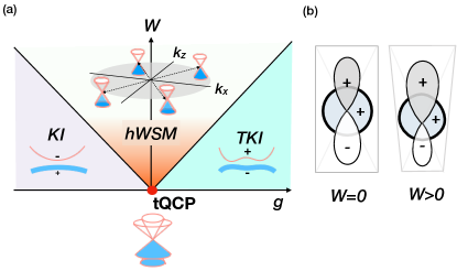
Figure 1: (a) Topological Quantum Critical Point (tQCP) at the nexus between normal and topological Kondo insulators (KI/TKIs) and heavy Weyl semimetals (hWSMs). $g$ and $W$ are the band tuning and inversion symmetry breaking parameters, respectively. At the tQCP, charge neutrality pins the bulk Dirac cone to the Fermi energy (occupied bands indicated by light blue). Finite $W>0$ splits the Dirac point into four symmetry-related Weyl points, pinned to the Fermi energy. (b) Breaking of inversion symmetry leads to a finite onsite hybridization $W>0$.

A preponderance of noncentrosymmetric heavy fermion materials offers an exciting opportunity to explore strongly interacting, or “heavy Weyl semimetals” (hWSMs)Xu et al. (2017); Lai et al. (2016). Four candidates have already come to light: CeRu₄Sn₆Guritanu et al. (2013), Ce₃Bi₄Pd₃Dzsaber et al. (2017), CeRu₄Sb₁₂Okamura et al. (2011); Shankar et al. (2016) and YbPtBiGuo et al. (2017). Optical measurements on CeRu₄Sn₆Guritanu et al. (2013) and transport measurements on CeRu₄Sb₁₂Okamura et al. (2011); Shankar et al. (2016) indicate anisotropic semimetallic behavior. More remarkably, the recent observation of a giant $T^{3}$ component to the specific heat of Ce₃Bi₄Pd₃Dzsaber et al. (2017) and YbPtBiGuo et al. (2017) reveals the presence of point-node excitations.

Recent density functional calculationsWissgott and Held (2016); Xu et al. (2017) confirm that heavy fermion systems are expected to host Weyl points with surface Fermi arcs. Lai et al.Lai et al. (2016) have recently proposed a tight-binding model for heavy Weyl semimetalsLai et al. (2016), predicting that the density of states near the Weyl nodes is strongly renormalized by the hybridization with f-electrons. These works raise a number of open questions:

• what is the relationship between heavy Weyl semimetals and topological Kondo insulators?

• beyond renormalization, what are the qualitative effects of strong interactions?

In this letter, we propose a simple a two-band model which links the emergence of heavy Weyl semi-metals at the topological quantum critical point (tQCP) between Kondo and topological Kondo insulators to the development of a parity-breaking on-site hybridization between $d$- and $f$-states in noncentrosymmetric Kondo lattices[Fig. 1(a)].

One of the qualitative effects predicted by our model, is the phenomenon of Kondo breakdown, whereby the loss of coordination of local moments at the surface leads to a reduction of the surface Kondo temperature. This phenomenon has been proposed as the origin of light surface quasiparticles observed in SmB₆Alexandrov et al. (2015). The analogous effect on the Fermi arcs causes them to reconfigure their geometry [Fig. 2] as a function of temperature, giving rise to a strong temperature dependence in the inter-surface cyclotron orbits Dai (2016); Potter et al. (2014); Moll et al. (2016).

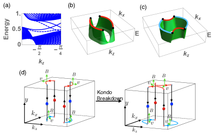
Figure 2: (a) Kondo Breakdown in a heavy Weyl semimetal, contrasting the spectrum before (solid lines) and after (dashed lines) surface Kondo breakdown as a function of $k_{z}$ at $k_{x}=0$. Surface spectrum (b) before and (c) after surface Kondo breakdown: red and blue lines indicate the Fermi arcs on the top and bottom surfaces respectively. Black dots indicate the projection of the Weyl nodes onto the surface. Parameters were taken to be $(t_{x},t_{y},t_{z},\mu,\alpha,V_{x},V_{y},V_{z},W_{2},b,\lambda)=(2,1,1,-6,-0.1,0.7,0.7,1.05,0.8,0.89,0.087)$ in Eq. (14). (d) Schematic of the Weyl orbits, where arrows indicate the quasiparticle trajectory.

Dzero et al. have emphasized that the spin-orbit driven topological behavior in heavy fermion systems derives from the odd-parity hybridization between $d$ ($\phi_{d}$) and $f$-orbitals ($\phi_{f}$)Mott (1974); Dzero et al. (2010, 2012) given by the Slater-Koster overlap integral

$$\tilde{V}_{\alpha\beta}({{\bf R}})=\int d^{3}x\phi^{*}_{d\alpha}({\bf x}-{\bf R}){\mathrm{V}}({\bf x})\phi_{f\beta}({\bf x}),$$ (1)

where ${\mathrm{V}}({\bf x})$ is the electronic potential. Inversion symmetry in centrosymmetric crystals fully eliminates the onsite hybridization between the opposite parity $d$ and $f$ states ($V_{\alpha\beta}(0)=0$) [Fig. 1(b)], and in momentum space, the residual intersite components of the hybridization then acquire the odd-in time, odd-in momentum, relativistic form $V_{\alpha\beta}({\bf k})\sim{\bf k}\cdot\vec{\sigma}$ near the high symmetry points. The band-crossing permitted by this nodal hybridization drives the formation of topological Kondo insulators. On the other hand, in non-centrosymmetric crystals, the asymmetric potential ${\rm V}({\bf x})\neq{\mathrm{V}}(-{\bf x})$ distorts the $f$ and $d$ orbitals and eliminates parity conservation, giving rise to a finite onsite d-f hybridization $W_{\alpha\beta}=\tilde{V}_{\alpha\beta}({\bf R}=0)$[Fig. 1(b)]. Under the influence of this perturbation, topological Kondo insulators become heavy Weyl semimetals as shown in Fig. 1(a). A minimal model for the hybridization that captures these features in a two-band model is obtained by generalizing the nearest-neighbor model introduced by Alexandrov, Coleman, and ErtenAlexandrov et al. (2015) (ACE) to include an additional onsite term as follows:

$$\tilde{V}({\bf R})_{\alpha\beta} = \left\{\begin{array}[]{lc}\displaystyle-{i}\vec{v}_{{\bf R}}\cdot{\bm{\sigma}}_{\alpha\beta},&\quad{{\bf R}\in\hbox{n.n.}}\\ {w}_{0}+i\vec{{w}}\cdot{\bm{\sigma}}&\quad{{\bf R}=0}.\end{array}\right.$$ (4)

where the vector $\vec{v}_{\bf R}=(v_{1}R_{1},v_{2}R_{2},v_{3}R_{3})$ describes the strength of the nearest neighbor hybridization while $w_{0}$ and $\vec{w}$ describe the inversion-symmetry breaking onsite hybridization terms, in a time-reversal invariant form.

II Model

We use a non-centrosymmetric modification of the ACE model Alexandrov et al. (2015)

$$H=\sum_{i,j,\sigma,\sigma^{\prime}}\Psi_{i\sigma}^{\dagger}\mathcal{H}_{ij,\sigma\sigma^{\prime}}\Psi_{j\sigma^{\prime}}+U\sum_{i}n_{if\uparrow}n_{if\downarrow},$$ (5)

where

$$\mathcal{H}_{ij,\sigma\sigma^{\prime}}=\left(\begin{array}[]{cc}(-t^{c}_{i,j}-\mu^{c}\delta_{ij})\delta_{\sigma\sigma^{\prime}}&\tilde{V}_{\sigma\sigma^{\prime}}({\bf R}_{i}-{\bf R}_{j})\\ \tilde{V}_{\sigma\sigma^{\prime}}({\bf R}_{i}-{\bf R}_{j})&(-t^{f}_{i,j}-\mu^{f}\delta_{ij})\delta_{\sigma\sigma^{\prime}}\end{array}\right).$$ (8)

Here $\Psi_{i\sigma}^{\dagger}=(c^{\dagger}_{i\sigma}$, $f^{\dagger}_{i\sigma})$ with $c^{\dagger}_{i\sigma}$ and $f^{\dagger}_{i\sigma}$ are the creation operators for conduction and f-electrons. $t^{c/f}_{ij}$ is the hopping amplitude and $\mu^{c/f}$ is the chemical potential for $c/f$ electrons. $U$ is the onsite Coulomb repulsion between f-electrons.

In the large $U$ limit, a slave-boson approach leads to the mean-field HamiltonianColeman (1987), $H=\sum_{\bf k}\Psi^{\dagger}({\bf k})\mathcal{H}({\bf k})\Psi({\bf k})+\mathcal{N}_{s}\lambda(|b|^{2}-Q)$ with

$$\mathcal{H}({\bf k})= \left(\begin{array}[]{cc}\epsilon_{c}({\bf k})-\mu&\sum_{j}V_{j}\sigma_{j}\sin k_{j}\\ \sum_{j}V_{j}\sigma_{j}\sin k_{j}&\epsilon_{f}({\bf k})+\lambda\end{array}\right)$$ (11)

$$+\left(\begin{array}[]{cc}0&W_{0}+i\vec{W}\cdot\vec{\sigma}\\ W_{0}-i\vec{W}\cdot\vec{\sigma}&0\end{array}\right).$$ (14)

$V_{i}=v_{i}b$ and $W_{i}={w}_{i}b$ are the renormalized hybridization terms, $b$ is the slave boson projection amplitude. The f-hopping amplitude becomes $\tilde{t}^{f}=b^{2}t^{f}$ The dispersion of the conduction electrons is taken as $\epsilon_{c}({\bf k})=-2\sum_{i}t_{i}\cos k_{i}$ and $\epsilon_{f}({\bf k})=\alpha\epsilon_{c}({\bf k})$ for simplicity. The constraint field $\lambda$ imposes the mean-field constraint $Q=n_{f}+b^{2}$ with $Q$ being the local conserved charge associated with the slave boson approach in the infinite $U$ limit, and is taken to be $Q=1$. $\mathcal{N}_{s}$ is the total number of sites. We solve the slave-boson mean-field Hamiltonian self-consistently [see Appendix A].

The spectrum of the Hamiltonian [Eq. (14)] is

$$E({\bf k})=h_{0}\pm\sqrt{h_{1}^{2}+W_{\mu}^{2}+\vec{V}_{{\bf k}}^{2}\pm 2\sqrt{W_{\mu}^{2}\ \vec{V}_{{\bf k}}^{2}-(\vec{W}\cdot\vec{V}_{{\bf k}})^{2}}},$$ (15)

where $h_{0/1}=\frac{1}{2}[\epsilon_{f}({\bf k})+\lambda\pm(\epsilon_{c}({\bf k})-\mu)]$, $W_{\mu}^{2}=W_{0}^{2}+\vec{W}^{2}$ and $\vec{V}_{{\bf k}}=(V_{1}\sin k_{1},V_{2}\sin k_{2},V_{3}\sin k_{3})$.

The energy spectrum has line or point nodes determined by the intersections between three surfaces: ${\cal S}_{I}$ where $h_{1}=0$, ${\cal S}_{II}$, where $(W_{\mu}^{2}-\vec{V}_{{\bf k}}^{2})^{2}=0$ and ${\cal S}_{III}$ where $\vec{W}\cdot\vec{V}_{{\bf k}}=0$. When there is no common intersection between these surfaces, the ground-state remains a fully gapped insulator. However, once $W$ exceeds a critical value, a semi-metallic state develops. There are two cases:

• Line-node semimetal ($\vec{W}=0$) for which the constraint ${\cal S}_{III}$ is trivial. Since ${\cal S}_{I}$ and ${\cal S}_{II}$ are spheroids that share the same center, they intersect to form two rings $\{r_{1},r_{2}\}={\cal S}_{I}\cap{\cal S}_{II}$ of gapless excitations [Fig. 3(a)] [see Appendix E for the detailed discussion].

• Weyl semimetal ($\vec{W}\neq 0$). Here ${\cal S}_{III}$ is the plane normal to $\vec{W}$, intersecting with rings $\{r_{1},r_{2}\}$ at four Weyl points [Fig. 3(b)].

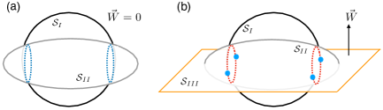
Figure 3: (a) A line-node semimetal: when $\vec{W}=0$, the line-node solution from Eq. (15) is determined by the intersections $\{r_{1},r_{2}\}={\cal S}_{I}\cap{\cal S}_{II}$ indic ated by blue lines. (b) A Weyl semimetal: When $\vec{W}\neq 0$, point-node solutions of Eq. (15), indicated by blue dots, develop at the intersections of plane ${\cal S}_{III}$ normal to $\vec{W}$ with the line-nodes, ${\cal S}_{I}\cap{\cal S}_{II}\cap{\cal S}_{III}$.

Time reversal and reflection symmetries play an important role in Weyl semimetals. Our model preserves time-reversal symmetry, $\mathcal{T}^{-1}\mathcal{H}({\bf k})\mathcal{T}=\mathcal{H}(-{\bf k})$, where $\mathcal{T}=i\sigma_{2}\mathcal{K}$ and $\mathcal{K}$ is the conjugation operator. In the absence of $W_{0}$, providing the inversion-symmetry breaking vector $\vec{W}=W\hat{l}$ points along a crystal axis $\hat{l}$, then the model also retains reflection symmetries in the two planes with normals $\hat{j}\neq\hat{l}$ perpendicular to $\hat{l}$. For our model, the reflection operator is $\mathcal{R}_{j}=\sigma_{j}\tau_{3}$ and $\mathcal{R}^{-1}_{j}\mathcal{H}({\bf k})\mathcal{R}_{j}=\mathcal{H}({{\bf k_{R}}})$, where ${\bf k_{R}}$ is the wavevector reflected in the plane perpendicular to $\hat{j}$ and ${\bm{\tau}}$ are the Pauli matrices in $c,f$ space. Suppose for example $\vec{W}=W_{2}\hat{y}$, then the energy spectrum has four Weyl points located in the $k_{y}=0$ plane, each related to one-another by time reversal and reflection symmetries $\mathcal{R}_{x}$ and $\mathcal{R}_{z}$.

The effective Hamiltonian near the Weyl points is obtained from Eq. (14) by projecting it onto the eigenvectors of the two central bands [see Appendix B]. For $\vec{W}=W_{2}\hat{y}$, we have four Weyl points $\vec{k}_{0}$, $R_{x}\vec{k}_{0}=(-k_{x0},0,k_{z0})$, $R_{z}\vec{k}_{0}=(k_{x0},0,-k_{z0})$, and $T\vec{k}_{0}=-\vec{k}_{0}$ related by reflection and time-reversal symmetries, respectively. The effective Hamiltonian can be expressed in a general form

$$\mathcal{H}_{\rm eff}(\vec{k}_{0},\delta{\bf k})= [A({\vec{k}_{0}})]_{i\alpha}\delta k_{i}\sigma_{\alpha}.$$ (16)

with implied summation on $i\in[x,y,z]$ and $\alpha\in[0,1,2,3]$ with $\sigma_{0}=\mathbb{I}_{2\times 2}$. Here $[A({\vec{k}_{0}})]_{i\alpha}$ is a three by four matrix defined at each Weyl point $\vec{k}_{0}$, each proportional to the hybridization amplitudes $V_{i}$ [see Appendix B]. These four effective Hamiltonians are related by reflection and time-reversal symmetries ($R_{x(z)}:\mathcal{H}_{\rm eff}({\vec{k}_{0}},\delta{\bf k})\to\mathcal{H}_{\rm eff}({R_{x(z)}\vec{k}_{0}},R_{x(z)}\delta{\bf k})$ and $T:\mathcal{H}_{\rm eff}({\vec{k}_{0}},\delta{\bf k})\to\mathcal{H}_{\rm eff}({-\vec{k}_{0}},-\delta{\bf k})$) which constrains the four Weyl points to lie at the same energy.

III Surface Kondo breakdown

We now examine the effect of “Kondo breakdown” on the Fermi arcs. The topological charges $C=\pm 1$ [see Appendix C] associated with the Weyl points give rise to the formation of Fermi arcs which link the projections of oppositely charged Weyl points onto the surface Brillouin zone (BZ). The analytic form of the localized Fermi arcs can be derived from the effective Hamiltonian [see Appendix D]. In the presence of interactions, the reduction in co-ordination number of the f-elections at the surface suppresses the surface Kondo temperature $T_{K}^{*}$ below that of the bulk, $T^{s}_{K}<T_{K}$. In the intermediate temperature regime $T^{s}_{K}<T<T_{K}$, the bulk is topological but the conduction electrons at the surface are liberated from the local moments, leading to surface Kondo breakdown. The surface Kondo breakdown scenario has been confirmed in inhomogeneous mean-field approachAlexandrov et al. (2015) and dynamical mean field calculations Peters et al. (2016). To model this effect, we suppress the slave boson amplitude $b$ to zero on the surface layer of hWSMs and recompute the Fermi arcs.

The effect of Kondo breakdown on the surface spectra for a $(010)$ slab geometry is shown in Figs. 2(a)-(c): we see that the intersections between two surface chiral modes sink beneath the Fermi sea. This effect causes the right and left chiral modes to bulge outwards, leading to a differential reconfiguration of the Fermi arcs on opposite surfaces as shown in Fig. 2(c). In fact, the detailed configuration of the Fermi arcs will in general depend on the microscopic parameters of the Hamiltonian. For example, in CeRu₄Sn₆ Xu et al. (2017), the nonequivalent cleavage surfaces are found to give rise to different configurations of Fermi arcs. This indicates that the Fermi arcs are sensitive to the surface morphologies and chemical potential. The configuration of the Fermi arcs will also be sensitive to the surface hybridization. Thus the surface Kondo breakdown introduces the reconfiguration of the Fermi arcs. The configuration of the Fermi arcs is a global property of the system, dependent on both bulk and surface properties. In particular, the configuration depends on the locations of the projected Weyl points on the surface BZ and the detailed dispersions of the surface spectrum. On the other hand, the topology of each Weyl point is a local property, with a generic form as described by Eq. (16). The finite topological charge $C=\pm 1$ of the Weyl point, ensures the formation of Fermi arcs which link with the projections of oppositely charged Weyl points on the surface BZ. However, this local property does not constrain the way the pairs of oppositely charged Weyl points are linked.

The reconfiguration of the Fermi arcs will have various distinct signatures in both angle-resolved photoemission spectroscopy and quantum oscillation measurements. In a field, quasiparticles on the surface move under the influence of the Lorentz force $\dot{\bf k}=-e{\bf v}_{\rm S}\times{\bf B}$, where ${\bf v}_{\rm S}$ is their velocity, processing from one projected Weyl point to another. When they reach a Weyl point, the gapless bulk chiral Landau level provides a transport channel to coherently move the quasiparticles between surfaces, giving rise to closed inter-plane Weyl orbits, Dai (2016); Potter et al. (2014) as shown in Fig. 2(d). Quantization of the Weyl orbital motion leads to discrete energy levels $E_{n}=\frac{\pi h(n+\gamma)v_{\rm B}}{L+\beta k_{0}/(eB)}$, where $k_{0}$ is the length of the Fermi arcs, $\mu$ is the chemical potential, $L$ is the thickness of the sample, $\gamma$ is a constant, and $\beta=v_{\rm B}/v_{\rm S}$ with $v_{\rm B}$ being the bulk velocity. Such Landau levels have been observed in Shubnikov-de Haas oscillations in Cd₃As₂, a weakly interacting Dirac semimetal which is the crystal-symmetry-protection analogy of a Weyl semimetalMoll et al. (2016).

One of the most dramatic consequences of the differential reconfiguration is the merger of two small orbits into a single large orbit as shown in Fig. 2(d), and the effect that will modify the quantum oscillations. Suppose the chemical potential is fixed to be $\mu$ and vary the magnetic field $B$, the $n$th energy level crosses the $\mu$ with the condition

$$\frac{1}{B_{n}}=\begin{cases}\frac{e}{\beta k_{0}}\left(\frac{v_{\rm B}\pi h}{\mu}(n+\gamma)-L\right),&T<T_{K}^{s}<T_{K}\\ \frac{e}{\beta^{\prime}(k_{0}^{\prime}+k_{1})}\left(\frac{v_{\rm B}\pi h}{\mu}(n+\gamma)-2L\right),&T_{K}^{s}<T<T_{K},\end{cases}$$ (17)

where $k_{0}^{\prime}$ and $k_{1}$ are the arc-lengths on the bottom and top surfaces respectively [see right panel in Fig. 2(d)], while $\beta^{\prime}=v_{\rm B}/v^{\prime}_{\rm S}$ with $v^{\prime}_{\rm S}$ being the surface velocity of quasiparticles with surface Kondo breakdown.

During the transition of surface Kondo breakdown, the spacing of the density of states as a function of $1/B$ has a dramatic change, $\omega_{B^{-1}}=\frac{e\pi hv_{\rm B}}{\beta\mu k_{0}}\to\frac{e\pi hv_{\rm B}}{\beta^{\prime}\mu(k^{\prime}_{0}+k_{1})}$. The magnetic field $1/B$ threshold of observing this oscillation also changes from $eL/\beta k_{0}\to 2eL/\beta^{\prime}(k^{\prime}_{0}+k_{1})$. The differential reconfiguration of the Fermi arc states can be detected by measuring the change of oscillation frequency and a threshold of the magnetic field in Shubnikov-de Haas oscillations.

IV Renormalization effects

The renormalized velocity of the Weyl semimetals described in Eq. (16) is proportional to the hybridization amplitude $V_{i}\propto\sqrt{T_{K}D}$ where $T_{K}$ is the Kondo temperature and $D$ is the band width of the conduction electronsColeman (2015). This “square-root” renormalization effect is weaker than that seen in heavy fermion metals, due to the hybridization origin of the nodes. From Ref. [Xu et al., 2017], the velocity of Weyl fermion in CeRu₄Sn₆ is $v^{*}\sim 0.2$ eVÅ. For the weakly interacting Weyl semimetals such as TaAsLv et al. (2015) and TaPXu et al. (2015), the velocity of Weyl fermion $v\sim 2-3$ eVÅ. The renormalization effect in hWSMs is about a factor of ten.

Many of the thermodynamic and transport properties in hWSMs are affected by this quasiparticle renormalization effect. One of the most dramatic effects, is the renormalization of the cubic specific heat. A large $T^{3}$ specific heat has been reported in the candidate hWSM materials Ce₃Bi₄Pd₃Dzsaber et al. (2017) and YbPtBiGuo et al. (2017). As pointed out by Lai et al.Lai et al. (2016) this significant enhancement of specific heat likely derives from the cubic dependence on renormalized velocity $C_{v}=\frac{\partial}{\partial T}\int\epsilon f(\epsilon)g(\epsilon)d\epsilon\propto(T/v^{*})^{3}$ with $g(\epsilon)=\frac{\epsilon^{2}}{2\pi^{2}v^{*3}}$ being the density of states. In addition to the specific heat, an enhancement of the high-field thermopowerSkinner and Fu (2017) is also expected. The high-field thermoelectric properties of the Weyl/Dirac semimetals contrast dramatically with those of doped semiconductors, with a thermopower that grows linearly, without saturation, in a the magnetic field, $\alpha:=\Delta V/\Delta T\propto BT/v^{*}$, where $\Delta V$ and $\Delta T$ are the voltage and temperature difference, respectively. The non-saturating behavior leads to a large thermopower which has been observed in weakly interacting Dirac semimetal Pb_1-xSn_xSeLiang et al. (2013). The high-field thermopower is thus enhanced by the mass renormalization in hWSMs.

V Conclusion and discussion

We have proposed a hybridization-driven model for heavy Weyl semimetals, arguing that the onsite hybridization between $f$ and $d$ orbitals in non-centrosymmetric crystals drives topological Kondo insulators into hWSMs. One of the effects of the strong interactions is surface Kondo breakdown, which leads to a reconfiguration of Fermi arcs on both surfaces that should appear in quantum oscillations, while the renormalization of velocity in hWSMs affects thermodynamic and transport properties.

There are a number of interesting new directions for research into hWSMs that deserve mention. One aspect that deserves exploration is the influence of non-symmorphic space group symmetries. According to topological band theoryBradlyn et al. (2016), such symmetries can lead to nodal points with much higher multiplicities, giving rise to a cluster of nested Dirac cones. A particularly interesting case is the candidate hWSM Ce₃Bi₄Pd₃, the space group No. $220$ ($I\bar{4}3d$) is expected to produce an eight-fold degenerate double Dirac point. These nodal lines are expected to give rise to “drumhead surface states”Matsuura et al. (2013); Burkov and Balents (2011); Bian et al. (2016) [see Appendix E], which can potentially cause charge/spin density wave and superconducting instabilities. A second interesting direction, is the possible use of molecular beam epitaxy (MBE) techniques Ishii et al. (2016), which open up the possibility of artificially engineered hWSMs where tuning the degree of inversion symmetry breaking can be used to explore the vicinity, and possible instabilities of the topological quantum critical pointYang et al. (2014); Isobe and Fu (2016).

Appendix A Self-consistent slave boson mean-field solutions

In the large $U$ limit, a slave-boson approach leads to the mean-field HamiltonianColeman (1987), $H=\sum_{\bf k}\Psi^{\dagger}({\bf k})\mathcal{H}({\bf k})\Psi({\bf k})+\mathcal{N}_{s}\lambda(|b|^{2}-Q)$ with

$$\mathcal{H}({\bf k})= \left(\begin{array}[]{cc}\epsilon_{c}({\bf k})-\mu&\sum_{j}V_{j}\sigma_{j}\sin k_{j}\\ \sum_{j}V_{j}\sigma_{j}\sin k_{j}&\epsilon_{f}({\bf k})+\lambda\end{array}\right)$$ (20)

$$+\left(\begin{array}[]{cc}0&W_{0}+i\vec{W}\cdot\vec{\sigma}\\ W_{0}-i\vec{W}\cdot\vec{\sigma}&0\end{array}\right).$$ (23)

$V_{i}=v_{i}b$ and $W_{i}={w}_{i}b$ are the renormalized hybridization terms, $b$ is the slave boson projection amplitude. The f-hopping amplitude becomes $\tilde{t}^{f}=b^{2}t^{f}$ The dispersion of the conduction electrons is taken as $\epsilon_{c}({\bf k})=-2\sum_{i}t_{i}\cos k_{i}$ and $\epsilon_{f}({\bf k})=\alpha\epsilon_{c}({\bf k})$ for simplicity. The constraint field $\lambda$ imposes the mean-field constraint $Q=n_{f}+b^{2}$ with $Q$ being the local conserved charge associated with the slave boson approach in the infinite $U$ limit, and is taken to be $Q=1$. $\mathcal{N}_{s}$ is the total number of sites.

The saddle point equations can be obtained from $\frac{\delta\langle H\rangle}{\delta b}=0$ and $\frac{\delta\langle H\rangle}{\delta\lambda}=0$.

$$\frac{1}{\mathcal{N}_{s}}\sum_{{\bf k},\sigma}\langle f^{\dagger}_{{\bf k},\sigma}f_{{\bf k},\sigma}\rangle+b^{2}=1$$ (24)

$$\frac{1}{2\mathcal{N}_{s}}\sum_{{\bf k},\sigma,i,j,\alpha,\beta}\{(v_{i}\sin k_{i}[\sigma_{i}]_{\alpha\beta}+w_{0}\delta_{\alpha\beta}+iw_{j}[\sigma_{j}]_{\alpha\beta})$$ (25)

$$\langle c^{\dagger}_{{\bf k},\alpha}f_{{\bf k},\beta}\rangle+h.c.\}+b(\lambda-\frac{1}{\mathcal{N}_{s}}\sum_{{\bf k},\sigma}\langle\tilde{\epsilon}_{f}({\bf k})f^{\dagger}_{{\bf k},\sigma}f_{{\bf k},\sigma}\rangle)=0,$$ (26)

where $\tilde{\epsilon}_{f}({\bf k})=\frac{1}{b^{2}}{\epsilon}_{f}({\bf k})$ is the bare spectrum of the f-electron.

In the paper we consider the case of non-zero on-site hybridization $w_{2}\neq 0$. For the specific calculations carried out in the paper, we have chosen the bare parameter values to be $(v_{x},v_{y},v_{z},w_{2},\alpha,t_{x},t_{y},t_{z},\mu)=(0.786,0.786,1.179,0.89,-0.126,2,1,1,-6)$, leading to a self-consistently determined slave boson amplitude and the constraint field with values $(b,\lambda)=(0.89,0.087)$.

Appendix B Effective two dimensional Hamiltonian near the Weyl points

Now we analyze the effective Hamiltonian around the Weyl points. We consider the inversion breaking hybridization $W_{2}\neq 0$ such that the Weyl points are located at $k_{y}=0$ plane. The locations of the Weyl points in momentum space satisfy

$$-2t_{x}\cos k_{x0}-2t_{z}\cos k_{z0}-(\mu+2t_{y})=0,$$

$$W_{2}^{2}=V_{1}^{2}\sin^{2}k_{x0}+V_{3}^{2}\sin^{2}k_{z0}.$$ (27)

We can expand the Hamiltonian around the Weyl points up to linear terms in ${\bf k}$.

$$\mathcal{H}(\delta{\bf k})\sim\mathcal{H}_{0}+\mathcal{H}_{1}(\delta{\bf k}),$$ (28)

where

$$\mathcal{H}_{0}=[V_{1}(\sin k_{x0})\sigma_{1}+V_{3}(\sin k_{z0})\sigma_{3}]\tau_{1}+W_{2}\sigma_{2}\tau_{2},$$ (29)

and

$$\mathcal{H}_{1}(\delta{\bf k})= \frac{1}{2}(1+\alpha)[2t_{x}\sin k_{x0}\delta k_{x}+2t_{z}\sin k_{z0}\delta k_{z}]\tau_{3}$$

$$+[V_{1}(\cos k_{x0}\delta k_{x})\sigma_{1}+V_{2}\delta k_{y}$$

$$+V_{3}(\cos k_{z0}\delta k_{z})\sigma_{3}]\tau_{1}.$$ (30)

Here we have dropped terms proportional to the identity matrix which only shift the spectrum without changing the band topology. To obtain the effective two-dimensional Hamiltonian in the vicinity of the Weyl points we first find two eigenvectors of $\mathcal{H}_{0}$ with zero energy,

$$|v_{1}\rangle= \frac{1}{\sqrt{2(V^{2}_{1,k_{x0}}+V^{2}_{3,k_{z0}})+2V_{1,k_{x0}}\sqrt{V^{2}_{1,k_{x0}}+V^{2}_{3,k_{z0}}}}}$$

$$\left(\begin{array}[]{c}V_{1,k_{x0}}+\sqrt{V^{2}_{1,k_{x0}}+V^{2}_{3,k_{z0}}}\\ 0\\ -V_{3,k_{z0}}\\ 0\end{array}\right),$$ (35)

$$|v_{2}\rangle= \frac{1}{\sqrt{2(V^{2}_{1,k_{x0}}+V^{2}_{3,k_{z0}})+2V_{1,k_{x0}}\sqrt{V^{2}_{1,k_{x0}}+V^{2}_{3,k_{z0}}}}}$$

$$\left(\begin{array}[]{c}0\\ V_{3,k_{z0}}\\ 0\\ V_{1,k_{x0}}+\sqrt{V^{2}_{1,k_{x0}}+V^{2}_{3,k_{z0}}}\end{array}\right).$$ (40)

where $V_{1(3),k_{x/z0}}=V_{1(3)}\sin k_{x(z)0}$,and $V_{2,k_{y0}}=V_{2}$ with $\vec{k}_{0}$ being the position of the Weyl point.

The effective two dimensional Hamiltonian is then obtained by projecting the Hamiltonian onto these eigenvalues, $[\mathcal{H}_{\rm eff}]_{i,j}=\langle v_{i}|\mathcal{H}_{1}(\delta{\bf k})|v_{j}\rangle$ with $i,j=1,2$, giving rise to

$$\mathcal{H}_{\rm eff}(\delta{\bf k})=-h_{0,\vec{k}_{0}}\sigma_{z}-V_{2,k_{y0}}\delta k_{y}\sigma_{x}+\frac{V_{1,k_{x0}}+\sqrt{V^{2}_{1,k_{x0}}+V^{2}_{3,k_{z0}}}}{V^{2}_{1,k_{x0}}+V^{2}_{3,k_{z0}}+V_{1,k_{x0}}\sqrt{V^{2}_{1,k_{x0}}+V^{2}_{3,k_{z0}}}}\left[V_{1,k_{x0}}\tilde{V}_{1,k_{x0}}\delta k_{x}+V_{3,k_{z0}}\tilde{V}_{3,k_{z0}}\delta k_{z}\right]\sigma_{y},$$ (41)

where $h_{0,\vec{k}_{0}}=\frac{1}{2}(1+\alpha)[2t_{x}\sin{k_{x0}\delta k_{x}}+2t_{z}\sin{k_{z0}\delta k_{z}}]$, and $\tilde{V}_{1(3),k_{x(z)0}}=V_{1(3)}\cos k_{x(z)0}$.

For simplicity, we express the Hamiltonian as

$$\mathcal{H}_{\rm eff}(\delta{\bf k})=(A\delta k_{x}+B\delta k_{z})\sigma_{z}+(C\delta k_{x}+D\delta k_{z})\sigma_{y}+E\delta k_{y}\sigma_{x},$$ (42)

where

$${A}=-\frac{1+\alpha}{2}(2t_{x}\sin k_{x0}),\quad{B}=-\frac{1+\alpha}{2}(2t_{z}\sin k_{z0})\quad{C}=\frac{V_{1,k_{x0}}+\sqrt{V^{2}_{1,k_{x0}}+V^{2}_{3,k_{z0}}}}{V^{2}_{1,k_{x0}}+V^{2}_{3,k_{z0}}+V_{1,k_{x0}}\sqrt{V^{2}_{1,k_{x0}}+V^{2}_{3,k_{z0}}}}V_{1,k_{x0}}\tilde{V}_{1,k_{x0}},$$

$${D}=\frac{V_{1,k_{x0}}+\sqrt{V^{2}_{1,k_{x0}}+V^{2}_{3,k_{z0}}}}{V^{2}_{1,k_{x0}}+V^{2}_{3,k_{z0}}+V_{1,k_{x0}}\sqrt{V^{2}_{1,k_{x0}}+V^{2}_{3,k_{z0}}}}V_{3,k_{z0}}\tilde{V}_{3,k_{z0}},\quad{E}=-V_{2,k_{y0}}.$$ (43)

Appendix C Topological invariance of the Weyl points—Berry curvature

The topological invariance of the Weyl points is the Berry curvature computed from a two-dimensional surface encircling the Weyl point. The definition of the Berry curvature is

$$C=\frac{i}{2\pi}\sum_{\alpha\in{\rm occ.}}\int d^{2}k\langle\partial_{k_{i}}u_{\alpha}|\partial_{k_{j}}u_{\alpha}\rangle-(k_{i}\leftrightarrow k_{j}),$$ (44)

where $u_{\alpha}$ are the occupied bands and the two dimensional integral is a closed surface around one Weyl point.

Now we compute the Berry curvature around the Weyl point by using Eq. (41). Without loss of generality, we define $\tilde{k}_{x}=A\delta k_{x}+B\delta k_{z}$, $\tilde{k}_{z}=C\delta k_{x}+D\delta k_{z}$, and $\tilde{k}_{y}=E\delta k_{y}$.

We now choose a fixed radius $R$ around the Weyl point with $R^{2}=\sum_{i=x,y,z}\tilde{k}_{i}^{2}$. The occupied band with energy $-R$ is

$$u_{-}(\theta,\phi)=\left(\begin{array}[]{c}-\sin\frac{\theta}{2}e^{-i\phi}\\ \cos\frac{\theta}{2}\end{array}\right),$$ (47)

where we parameterize $\tilde{k}_{z}=R\cos\theta$, $\tilde{k}_{x}=R\sin\theta\cos\phi$, and $\tilde{k}_{y}=R\sin\theta\sin\phi$.

The only non-vanishing component of the Berry connection is

$$A_{\phi}=\frac{1}{R\sin\theta}\langle u_{-}(\theta,\phi)|\partial_{\phi}u_{-}(\theta,\phi)\rangle=\frac{i}{2R}\cot\theta.$$ (48)

The Berry curvature around the Weyl point is then

$$C=\frac{i}{2\pi}\int_{\rm sphere}ds(\nabla\times\vec{A})=\frac{i}{2\pi}\int R^{2}\sin\theta d\theta d\phi\frac{-i}{2R^{2}}=1.$$ (49)

The Berry curvature of teh the other time-reversal related Weyl points at $-\vec{k}_{0}$, is $C=-1$.

Appendix D Fermi arc states in the effective Hamiltonian

We analyze the Fermi arc state from the effective two-dimensional Hamiltonian in Eq. (41). In the presence of $(010)$ surface, the effective Hamiltonian around the Weyl point is expressed as

$$\mathcal{H}_{\rm eff.}=\left(\begin{array}[]{cc}A\delta k_{x}+{B}\delta k_{z}&-i{C}\delta k_{x}-i{D}\delta k_{z}-i{E}\partial_{y}\\ iC\delta k_{x}+i{D}\delta k_{z}-i{E}\partial_{y}&-{A}\delta k_{x}-{B}\delta k_{z}\end{array}\right).$$ (52)

We consider a cylindrical surface surrounding the Weyl point with radius $k_{0}$. The effective Hamiltonian becomes

$$\mathcal{H}_{\rm eff.}=\left(\begin{array}[]{cc}Ak_{0}\cos\theta+{B}k_{0}\sin\theta&-ik_{0}\sqrt{{C}^{2}+{D}^{2}}\cos(\theta-\phi)-i{E}\partial_{y}\\ ik_{0}\sqrt{{C}^{2}+{D}^{2}}\cos(\theta-\phi)-iE\partial_{y}&-{A}k_{0}\cos\theta-{B}k_{0}\sin\theta\end{array}\right),$$ (55)

where $\phi=\cos^{-1}\frac{C}{\sqrt{C^{2}+D^{2}}}$, $\delta k_{x}=k_{0}\cos\theta$, and $\delta k_{z}=k_{0}\sin\theta$.

There are two boundary states on this cylinder surrounding the Weyl point

$$u_{y>0}=\left(\begin{array}[]{c}1\\ 0\end{array}\right)\sqrt{2\kappa}e^{-\kappa y}\quad{\rm with}\quad E_{R}(\theta)={A}k_{0}\cos\theta+Bk_{0}\sin\theta,$$ (58)

$$u_{y<0}=\left(\begin{array}[]{c}0\\ 1\end{array}\right)\sqrt{2\kappa}e^{\kappa y}\quad{\rm with}\quad E_{L}(\theta)=-{A}k_{0}\cos\theta-Bk_{0}\sin\theta,$$ (61)

where $\kappa=-\frac{k_{0}}{E}\sqrt{{C}^{2}+{D}^{2}}\cos(\theta-\phi)>0$. These boundary states are the origin of the Fermi arc states.

Appendix E Time-reversal symmetric nodal ring semimetallic phase

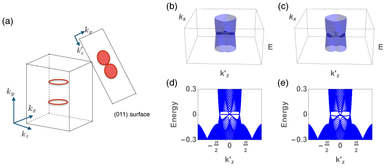
Figure 4: (a) Schematic plot of the bulk nodal rings centered at $k_{y}$ axis. On the $(011)$ surface, the surface flat bands will emerge inside the circles which are the projection of the bulk nodal rings. The surface spectrum as a function of $(k_{x},k^{\prime}_{z}=\frac{1}{\sqrt{2}}(k_{z}-k_{y}))$ from the Hamiltonian Eq. (14) with $(t_{x},t_{y},t_{z},\mu,\alpha,W_{x},W_{y},W_{z},W_{0})=(2,1,1,-6.5,-0.1,2,2,2,1.8)$. (b) in the absence of surface Kondo breakdown and (c) in the presence of surface Kondo breakdown. The surface spectrum as a function of $k^{\prime}_{z}=\frac{1}{\sqrt{2}}(k_{z}-k_{y})$ at $k_{x}=0$, (d) in the absence of surface Kondo breakdown and (e) in the presence of surface Kondo breakdown.

The Hamiltonian of hWSMs with non-vanishing $W_{0}$ can be expressed as

$$\mathcal{H}({\bf k})=\mathcal{H}_{0}({\bf k})+\mathcal{H}_{1}({\bf k}),$$ (62)

where $\mathcal{H}_{0}({\bf k})=\frac{1}{2}(\epsilon_{c}({\bf k})+\epsilon_{f}({\bf k}))\sigma_{0}\tau_{0}$ and $\mathcal{H}_{1}({\bf k})=\frac{1}{2}(\epsilon_{c}({\bf k})-\epsilon_{f}({\bf k}))\sigma_{0}\tau_{3}+\sum_{i=1,2,3}V_{i}\sin k_{i}\sigma_{i}\tau_{1}+W_{0}\tau_{1}.$$\mathcal{H}_{1}({\bf k})$ has a chiral symmetry, $\mathcal{S}^{-1}\mathcal{H}({\bf k})\mathcal{S}=-\mathcal{H}({\bf k})$, where $\mathcal{S}=\tau_{2}$. In the presence of chiral symmetry, one can off-block diagonalize $\mathcal{H}_{1}({\bf k})$ by a unitary transformation, $\mathcal{V}^{\dagger}\mathcal{H}_{1}({\bf k})\mathcal{V}=\tilde{\mathcal{H}_{1}}({\bf k})$, where

$$\mathcal{V}=\frac{1}{\sqrt{2}}\left(\begin{array}[]{cc}\mathbb{I}_{2\times 2}&i\mathbb{I}_{2\times 2}\\ i\mathbb{I}_{2\times 2}&\mathbb{I}_{2\times 2}\end{array}\right),\quad\tilde{\mathcal{H}}({\bf k})_{1}=\left(\begin{array}[]{cc}0&D({\bf k})\\ D^{\dagger}({\bf k})&0\end{array}\right),$$ (67)

with $D({\bf k})=i(\epsilon_{c}({\bf k})-\epsilon_{f}({\bf k}))+2\sum_{i}V_{i}\sin k_{i}\sigma_{i}+m_{0}$. The eigenvectors of $\tilde{\mathcal{H}}({\bf k})$ satisfy

$$\left(\begin{array}[]{cc}0&D({\bf k})\\ D^{\dagger}({\bf k})&0\end{array}\right)\left(\begin{array}[]{c}\chi^{\pm}({\bf k})\\ \eta^{\pm}({\bf k})\end{array}\right)=\pm\lambda({\bf k})\left(\begin{array}[]{c}\chi^{\pm}({\bf k})\\ \eta^{\pm}({\bf k})\end{array}\right).$$ (74)

These eigenvectors are also the eigenvector of $\mathcal{H}_{0}({\bf k})$ and they determine the topological invariant. We pick $\chi^{\pm}({\bf k})=\frac{1}{\sqrt{2}}u({\bf k})$, Then Eq. (74) leads to $\eta^{\pm}({\bf k})=\pm\frac{1}{\sqrt{2}}\frac{1}{\lambda({\bf k})}D^{\dagger}({\bf k})u({\bf k})$. The flat band Hamiltonian $\mathcal{Q}({\bf k})$can be obtained from the projector

$$\mathcal{Q}({\bf k})= \mathbb{I}-2\sum_{\alpha\in{\rm occ.}}|u_{\alpha}({\bf k})\rangle\langle u_{\alpha}({\bf k})|$$

$$= \mathbb{I}-\left(\begin{array}[]{c}u({\bf k})\\ -\frac{1}{\lambda({\bf k})}D^{\dagger}({\bf k})u({\bf k})\end{array}\right)\left(\begin{array}[]{cc}u^{\dagger}({\bf k})&-\frac{1}{\lambda({\bf k})}u^{\dagger}({\bf k})D({\bf k})\end{array}\right)$$ (78)

$$= \frac{1}{\lambda({\bf k})}\left(\begin{array}[]{cc}0&u({\bf k})u^{\dagger}({\bf k})D({\bf k})\\ D^{\dagger}({\bf k})u({\bf k})u^{\dagger}({\bf k})&0\end{array}\right)$$ (81)

$$= \left(\begin{array}[]{cc}0&q({\bf k})\\ q^{\dagger}({\bf k})&0\end{array}\right).$$ (84)

The topological invariance of the nodal ring is characterized by a winding number of a one-dimensional loop encircling the ring. The winding number can be calculated from the q-matrix integral

$$\nu=\frac{1}{2\pi i}\oint_{\mathcal{L}}d{\bf k}{\rm Tr}[q^{-1}({\bf k})\partial_{\bf k}q({\bf k})].$$ (85)

In our model, the winding number of the nodal rings is $\nu=\pm 1$, which leads to surface flat bands bounded by the nodal rings projected on the surface Brillouin zoneBurkov and Balents (2011); Matsuura et al. (2013). As shown schematically in Fig. 4(a), two nodal rings are centered along $k_{y}$ axis. On $(011)$ surface, the flat band surface states emerge inside the bulk rings projected on the $(011)$ surface Brillouin zone.

Finally, we have investigated the Kondo breakdown on these surface flat bands, summarizing the results in 4. In the absence of the surface Kondo breakdown, the surface flat bands emerge on $(011)$ surface (Fig. 4(b) and (d)). . In the presence of the surface Kondo breakdown, the surface flat bands sink beneath the Fermi sea as shown in Fig. 4(c) and (e).

References

- Mott (1974) N. Mott, Philosophical Magazine 30, 403 (1974).
- Dzero et al. (2010) M. Dzero, K. Sun, V. Galitski, and P. Coleman, Phys. Rev. Lett. 104, 106408 (2010).
- Dzero et al. (2012) M. Dzero, K. Sun, P. Coleman, and V. Galitski, Phys. Rev. B 85, 045130 (2012).
- Alexandrov et al. (2013) V. Alexandrov, M. Dzero, and P. Coleman, Phys. Rev. Lett. 111, 226403 (2013).
- Lu et al. (2013) F. Lu, J. Zhao, H. Weng, Z. Fang, and X. Dai, Phys. Rev. Lett. 110, 096401 (2013).
- Dzero et al. (2016) M. Dzero, J. Xia, V. Galitski, and P. Coleman, Annual Review of Condensed Matter Physics 7, 249 (2016), arXiv:1506.05635 [cond-mat.str-el] .
- Jiang et al. (2013) J. Jiang, S. Li, T. Zhang, Z. Sun, F. Chen, Z. R. Ye, M. Xu, Q. Q. Ge, S. Y. Tan, X. H. Niu, M. Xia, B. P. Xie, Y. F. Li, X. H. Chen, H. H. Wen, and D. L. Feng, Nat. Commun. 4, 3010 (2013).
- Neupane et al. (2013) M. Neupane, N. Alidoust, S.-Y. Xu, T. Kondo, Y. Ishida, D. J. Kim, C. Liu, I. Belopolski, Y. J. Jo, T.-R. Chang, H.-T. Jeng, T. Durakiewicz, L. Balicas, H. Lin, A. Bansil, S. Shin, Z. Fisk, and M. Z. Hasan, Nat. Commun. 4, 2991 (2013).
- Xu et al. (2013) N. Xu, X. Shi, P. K. Biswas, C. E. Matt, R. S. Dhaka, Y. Huang, N. C. Plumb, M. Radović, J. H. Dil, E. Pomjakushina, K. Conder, A. Amato, Z. Salman, D. M. Paul, J. Mesot, H. Ding, and M. Shi, Phys. Rev. B 88, 121102 (2013).
- Frantzeskakis et al. (2013) E. Frantzeskakis, N. de Jong, B. Zwartsenberg, Y. K. Huang, Y. Pan, X. Zhang, J. X. Zhang, F. X. Zhang, L. H. Bao, O. Tegus, A. Varykhalov, A. de Visser, and M. S. Golden, Phys. Rev. X 3, 041024 (2013).
- Murakami (2007) S. Murakami, New Journal of Physics 9, 356 (2007), arXiv:0710.0930 .
- Wan et al. (2011) X. Wan, A. M. Turner, A. Vishwanath, and S. Y. Savrasov, Phys. Rev. B 83, 205101 (2011).
- Burkov and Balents (2011) A. A. Burkov and L. Balents, Phys. Rev. Lett. 107, 127205 (2011).
- Xu et al. (2015) S.-Y. Xu, I. Belopolski, D. S. Sanchez, C. Zhang, G. Chang, C. Guo, G. Bian, Z. Yuan, H. Lu, T.-R. Chang, P. P. Shibayev, M. L. Prokopovych, N. Alidoust, H. Zheng, C.-C. Lee, S.-M. Huang, R. Sankar, F. Chou, C.-H. Hsu, H.-T. Jeng, A. Bansil, T. Neupert, V. N. Strocov, H. Lin, S. Jia, and M. Z. Hasan, Science Advances 1, e1501092 (2015), arXiv:1508.03102 [cond-mat.mes-hall] .
- Weng et al. (2015) H. Weng, C. Fang, Z. Fang, B. A. Bernevig, and X. Dai, Phys. Rev. X 5, 011029 (2015).
- Huang et al. (2015) S.-M. Huang, S.-Y. Xu, I. Belopolski, C.-C. Lee, G. Chang, B. Wang, N. Alidoust, G. Bian, M. Neupane, C. Zhang, S. Jia, A. Bansil, H. Lin, and M. Z. Hasan, Nat. Commun. 6, 7373 (2015).
- Xu et al. (2017) Y. Xu, C. Yue, H. Weng, and X. Dai, Phys. Rev. X 7, 011027 (2017).
- Lai et al. (2016) H.-H. Lai, S. E. Grefe, S. Paschen, and Q. Si, ArXiv e-prints (2016), arXiv:1612.03899 [cond-mat.str-el] .
- Guritanu et al. (2013) V. Guritanu, P. Wissgott, T. Weig, H. Winkler, J. Sichelschmidt, M. Scheffler, A. Prokofiev, S. Kimura, T. Iizuka, A. M. Strydom, M. Dressel, F. Steglich, K. Held, and S. Paschen, Phys. Rev. B 87, 115129 (2013).
- Dzsaber et al. (2017) S. Dzsaber, L. Prochaska, A. Sidorenko, G. Eguchi, R. Svagera, M. Waas, A. Prokofiev, Q. Si, and S. Paschen, Phys. Rev. Lett. 118, 246601 (2017).
- Okamura et al. (2011) H. Okamura, R. Kitamura, M. Matsunami, H. Sugawara, H. Harima, H. Sato, T. Moriwaki, Y. Ikemoto, and T. Nanba, Journal of the Physical Society of Japan 80, 084718 (2011), arXiv:1103.0811 [cond-mat.str-el] .
- Shankar et al. (2016) A. Shankar, D. P. Rai, S. Chettri, R. Khenata, and R. K. Thapa, Journal of Solid State Chemistry France 240, 126 (2016).
- Guo et al. (2017) C. Y. Guo, F. Wu, M. Smidman, F. Steglich, and H. Q. Yuan, ArXiv e-prints (2017), arXiv:1710.05522 [cond-mat.str-el] .
- Wissgott and Held (2016) P. Wissgott and K. Held, European Physical Journal B 89, 5 (2016), arXiv:1505.02055 [cond-mat.str-el] .
- Alexandrov et al. (2015) V. Alexandrov, P. Coleman, and O. Erten, Phys. Rev. Lett. 114, 177202 (2015).
- Dai (2016) X. Dai, Nat Phys 12, 727 (2016).
- Potter et al. (2014) A. C. Potter, I. Kimchi, and A. Vishwanath, Nature Communications 5, 5161 (2014).
- Moll et al. (2016) P. J. W. Moll, N. L. Nair, T. Helm, A. C. Potter, I. Kimchi, A. Vishwanath, and J. G. Analytis, Nature (London) 535, 266 (2016), arXiv:1505.02817 [cond-mat.mes-hall] .
- Coleman (1987) P. Coleman, Phys. Rev. B 35, 5072 (1987).
- Peters et al. (2016) R. Peters, T. Yoshida, H. Sakakibara, and N. Kawakami, Phys. Rev. B 93, 235159 (2016).
- Coleman (2015) P. Coleman, Introduction to Many-Body Physics (Cambridge University Press, 2015).
- Lv et al. (2015) B. Q. Lv, H. M. Weng, B. B. Fu, X. P. Wang, H. Miao, J. Ma, P. Richard, X. C. Huang, L. X. Zhao, G. F. Chen, Z. Fang, X. Dai, T. Qian, and H. Ding, Physical Review X 5, 031013 (2015), arXiv:1502.04684 [cond-mat.mtrl-sci] .
- Skinner and Fu (2017) B. Skinner and L. Fu, ArXiv e-prints (2017), arXiv:1706.06117 [cond-mat.str-el] .
- Liang et al. (2013) T. Liang, Q. Gibson, J. Xiong, M. Hirschberger, S. P. Koduvayur, R. J. Cava, and N. P. Ong, Nature Communications 4, 2696 (2013), arXiv:1307.4022 [cond-mat.str-el] .
- Bradlyn et al. (2016) B. Bradlyn, J. Cano, Z. Wang, M. G. Vergniory, C. Felser, R. J. Cava, and B. A. Bernevig, Science 353 (2016), 10.1126/science.aaf5037, http://science.sciencemag.org/content/353/6299/aaf5037.full.pdf .
- Matsuura et al. (2013) S. Matsuura, P.-Y. Chang, A. P. Schnyder, and S. Ryu, New Journal of Physics 15, 065001 (2013), arXiv:1212.2673 [cond-mat.supr-con] .
- Bian et al. (2016) G. Bian, T.-R. Chang, H. Zheng, S. Velury, S.-Y. Xu, T. Neupert, C.-K. Chiu, S.-M. Huang, D. S. Sanchez, I. Belopolski, N. Alidoust, P.-J. Chen, G. Chang, A. Bansil, H.-T. Jeng, H. Lin, and M. Z. Hasan, Phys. Rev. B 93, 121113 (2016).
- Ishii et al. (2016) T. Ishii, R. Toda, Y. Hanaoka, Y. Tokiwa, M. Shimozawa, Y. Kasahara, R. Endo, T. Terashima, A. H. Nevidomskyy, T. Shibauchi, and Y. Matsuda, Phys. Rev. Lett. 116, 206401 (2016).
- Yang et al. (2014) B.-J. Yang, E.-G. Moon, H. Isobe, and N. Nagaosa, Nat Phys 10, 774 (2014).
- Isobe and Fu (2016) H. Isobe and L. Fu, Phys. Rev. B 93, 241113 (2016).