Image Compression: Sparse Coding vs. Bottleneck Autoencoders

Abstract

Bottleneck autoencoders have been actively researched as a solution to image compression tasks. However, we observed that bottleneck autoencoders produce subjectively low quality reconstructed images. In this work, we explore the ability of sparse coding to improve reconstructed image quality for the same degree of compression. We observe that sparse image compression produces visually superior reconstructed images and yields higher values of pixel-wise measures of reconstruction quality (PSNR and SSIM) compared to bottleneck autoencoders. In addition, we find that using alternative metrics that correlate better with human perception, such as feature perceptual loss and the classification accuracy, sparse image compression scores up to 18.06% and 2.7% higher, respectively, compared to bottleneck autoencoders. Although computationally much more intensive, we find that sparse coding is otherwise superior to bottleneck autoencoders for the same degree of compression.

I Introduction

Image compression methods have significant practical and commercial interest and have been the topic of extensive research. Thumbnail images contain higher frequencies and much less redundancy, which makes them more difficult to compress compared to high-resolution images. A lot of research has been focused on improving the compression of thumbnails [8, 14, 9].

Bottleneck autoencoders achieve compression by using feed-forward artificial neural networks to reduce the dimensionality of the input data. The basic principles underlying convolutional and fully connected feed-forward neural networks, including bottleneck autoencoders, have been known for years [8, 11, 13].

Sparse coding algorithms use an overcomplete set of non-orthogonal basis functions (feature vectors) to find a sparse combination of non-zero activation coefficients that most accurately reconstruct each input image. Sparse coding image compression combines sparse coding with the ideas of downsampling and compressive sensing [7, 3, 5]: 1) a subset of the original pixels are used as a compressed image, 2) a minimal set of generators that explains the pixels in the compressed image is identified, and 3) the missing pixel values are inferred.

The peak-signal-to-noise ratio (PSNR) and the structural similarity index measure (SSIM) are two commonly used pixel-level image quality metrics. Both PSNR and SSIM fail to capture differences at the feature level and correlate poorly with human perception of image quality. Several researchers have therefore attempted to define alternative measures of compression quality based on the similarity of the features extracted from the reconstructed and original images and have shown that these alternative measures correlate better with human subjective perception [10, 4, 12]. We further introduce a new feature-based measure of compression quality based on loss of classification accuracy, in which compressed images are labeled using TensorFlow’s CIFAR-10 DCNN classifier [2] and the results compared to the baseline performance achieved on the original images.

In this work we apply bottleneck autoencoders and sparse coding approaches to the compression of thumbnail images and use both subjective, pixel-level and feature-based criteria for evaluating reconstructed image quality. We report that sparse coding with random dropout masks produces subjectively superior reconstructed images along with lower feature perceptual loss and higher classification accuracy but yields lower values of pixel-wise metrics such as PSNR and SSIM compared to the bottleneck autoencoders. However, sparse coding with a checkerboard mask yields superior performance as measured by all three of the above criteria.

II Methods

II-A Sparse Coding

Given an overcomplete basis, sparse coding algorithms seek to identify the minimal set of generators that most accurately reconstruct each input image. In neural terms, each neuron is a generator that adds its associated feature vector to the reconstructed image with an amplitude equal to its activation. For any particular input image, the optimal sparse representation is given by the vector of neural activations that minimizes both image reconstruction error and the number of neurons with non-zero activity. Formally, finding a sparse representation involves finding a minimum of the following cost function:

$$E(\ \overrightarrow{I},\phi,\ \overrightarrow{a})=\min\limits_{\{\overrightarrow{a},\,\phi\}}\left[\,\frac{1}{2}||\overrightarrow{I}-\phi*\overrightarrow{a}||^{2}+\lambda||\overrightarrow{a}||_{1}\right],$$ (1)

In Eq. (1), $\overrightarrow{I}$ is an image unrolled into a vector, and $\phi$ is a dictionary of feature kernels that are convolved with the sparse representation $\overrightarrow{a}$. The factor $\lambda$ is a tradeoff parameter; larger $\lambda$ values encourage greater sparsity (fewer non-zero coefficients) at the cost of greater reconstruction error. Both the sparse representation $\overrightarrow{a}$ and the dictionary of feature kernels $\phi$ can be determined by a variety of standard optimization methods. Our approach to compute a sparse representation for a given input image is based on a convolutional generalization of a rectifying Locally Competitive Algorithm (LCA) [6]. Once a sparse representation for a given input image has been found, the basis elements associated with non-zero activation coefficients are adapted according to a local Hebbian learning rule (with a momentum term for faster convergence) that further reduces the remaining reconstruction error. Starting with random basis elements, dictionary learning was performed via Stochastic Gradient Descent (SGD). This training procedure can learn to factor a complex, high-dimensional natural image into an overcomplete set of basis vectors that capture the high-dimensional correlations in the data.

[width=]sparse

(a) Sparse coding second line

[width=]bottleneck

(b) Bottleneck autoencoder

Figure 1: (a) Overcomplete representation with pixel dropout (black dots); (b) Undercomplete representation.

The sparse coding based image compression architecture is illustrated in Figure 1(a), where the input layer (left) is the original image, the hidden layer (middle) is its sparse representation, and the output layer (right) is the image reconstruction. The white pixels from the input layer are the compressed representation of the original image and black pixels are the omitted pixels of the original image. To summarize, image compression based on sparse coding involves two distinct steps: 1) Compression: a subset of the pixels (white circles) is used as a compressed representation of the original image. 2) Decompression: a minimal subset of pre-trained generators that explains the compressed representation is identified, and the missing pixel values are inferred from these generators.

During training, the sparse representation $\overrightarrow{a}$ is found using only the preserved pixel values. The omitted pixels do not contribute to the minimization of the cost function with respect to $\overrightarrow{a}$. Then $\overrightarrow{a}$ is used to update the dictionary of generators $\phi$ in order to reconstruct the original image, including the masked pixels, with minimal error.

We evaluated several sparse coding models which included a variety of structural elements such as convolutional layers, fully connected layers and multi-scale dictionaries. To facilitate comparison, each model contained the same total number of neurons. We found that the best performance was achieved by a model consisting of a single convolutional layer containing 1024 features with a patch size of $16\times 16$ pixels and a stride of 2 ($\simeq 42.6$ times overcomplete).

To determine the optimum percentage of non-zero activity, or optimal tradeoff parameter $\lambda$, for our sparse coding model, we trained our network for one epoch on 9 different $\lambda$ values using the single layer sparse convolutional model. We found that for the optimum value of $\lambda$ for our network, the average percentage of active neurons is 1.37% (see Figure 2). Our sparse coding image compression results used this single sparse convolutional model with the aforementioned optimal level of sparsity.

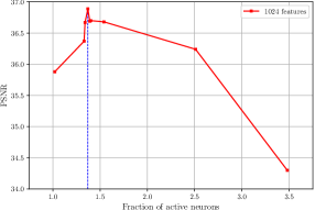
Figure 2: PSNR as a function of sparsity (fraction of active neurons) for various values of the tradeoff parameter $\lambda$.

II-B Bottleneck Autoencoder

The bottleneck autoencoder architecture is illustrated in Figure 1(b). This structure includes one input layer (left), one or more hidden layers (middle), and one output layer (right). The input and output layers contain the same number of neurons, where the output layer aims to reconstruct the input. Image compression is achieved by restricting the number of neurons in the smallest hidden layer (the bottleneck) to contain half the number of neurons of the input layer to achieve a 2:1 compression ratio. We evaluated several bottleneck autoencoder models such as fully connected models, convolutional models, and multi-scaled models, and found that a model combining one convolutional layer with a stride of 4 and one fully connected layer, each containing the same number of neurons ($1/4$ the number of pixels in the thumbnails), provides higher reconstructed image quality over other bottleneck models. The bottleneck autoencoder network finds the optimal hidden layer features across the training set of input images, that minimize the image reconstruction error. In the simplest case, as illustrated in Figure 1(b), the model minimizes the following energy function:

$$\begin{split}E(x;W,b,W^{\prime},b^{\prime})&=||x-x^{\prime}||^{2}\\ &=||x-\sigma(W^{\prime}(\sigma(Wx+b))+b^{\prime})||^{2}\end{split}$$ (2)

In Eq. (2), $x$ is the input image, $x^{\prime}$ is the reconstructed image, $\sigma$ is the ReLU activation function. $W$ and $b$ are the encoder’s weights matrix and a bias vector, $W^{\prime}$ and $b^{\prime}$ are the decoder’s weights matrix and a bias respectively.

In this type of neural network architecture, a large number of input neurons is fed into a smaller number of neurons in the hidden layer, which works as the compressor. This structured bottleneck layer could be treated as a nonlinear mapping of input features. The decompressor then reconstructs the compressed image back to the neurons in the output layer using the same weights as the compressor. The bottleneck autoencoder model employs SGD with momentum to train optimal values of the weights and bias after being randomly initialized. The bottleneck autoencoder is designed to preserve only those features that best describe the original image and shed redundant information.

III Results

In this work, we compared bottleneck autoencoders with two sparse coding approaches. For sparse coding we masked $50\%$ of the pixels either randomly or arranged in a checkerboard pattern to achieve a 2:1 compression ratio. The random mask is regenerated for every image batch whereas the checkerboard mask is fixed. In order to evaluate and compare the quality of the proposed sparse coding and bottleneck autoencoder image compression models, we used PetaVision[1], an open source neural simulation toolbox that enables multi-node, multi-core and GPU accelerated high-performance implementations of sparse solvers derived from LCA as well as conventional neural network models. We use the CIFAR-10 dataset, which consists of 50,000 $32\times 32$ images for training and 10,000 $32\times 32$ images for testing. Category labels were not used in this study.

III-A Image Compression

We first evaluated the quality of the reconstructed images from sparse coding and the bottleneck autoencoder using subjective human perceptual judgments. Figure 3 shows examples of sparse coding and bottleneck autoencoder based image compression. Subjective examination reveals that the reconstructed images from sparse coding with either random or checkerboard mask exhibit less noise, has a smoother background, and results in more natural looking reconstructions than images reconstructed from the bottleneck autoencoder. Sparse coding with a random mask preserves less fine detail compared to the bottleneck autoencoder whereas sparse coding with a checkerboard mask preserves both background and fine details much better than both the other methods. Overall, the images compressed using sparse coding with a checkerboard mask are almost visually indistinguishable from the original images.

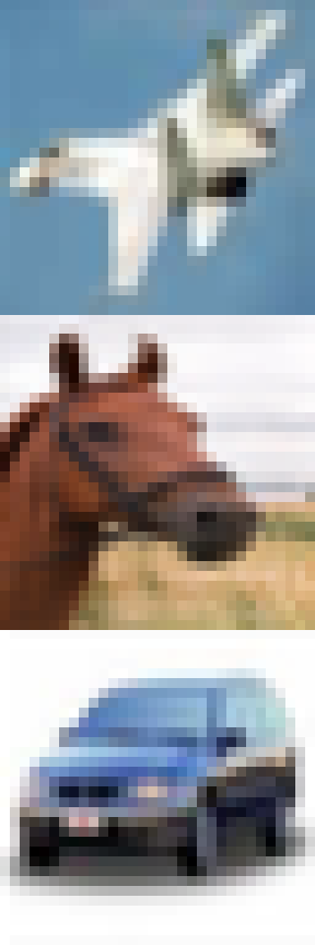
(a)

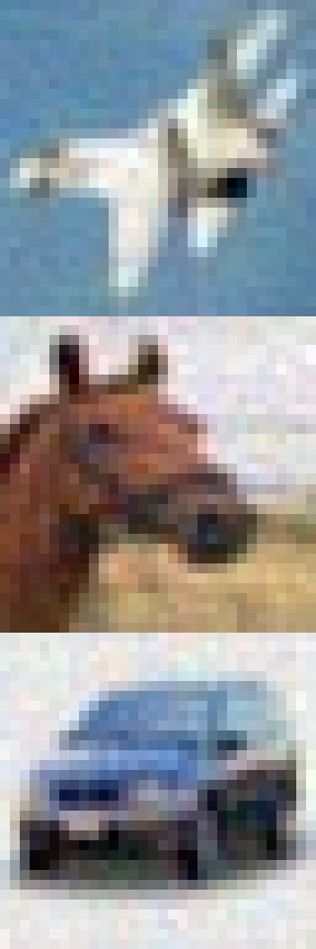
(b)

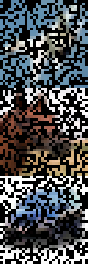
(c)

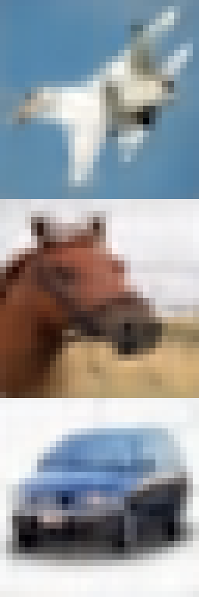
(d)

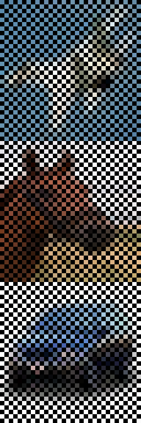
(e)

(f)

Figure 3: (a) Original images; (b) Reconstructed images: Bottleneck autoencoder; (c) Random masks in which ${\simeq}$50% of the original pixels are omitted; (d) Reconstructed images: Sparse coding with random mask; (e) Checkerboard masks in which 50% of the original pixels are omitted; (f) Reconstructed images: Sparse coding with checkerboard mask.

III-B Pixel-wise Loss in Image Space

We used two well-known pixel-wise image quality metrics: the peak-signal-to-noise ratio (PSNR) and the structural similarity index measure (SSIM) to evaluate the reconstructed images from either sparse coding or the bottleneck autoencoder.

TABLE I: Image Reconstruction

Methods	PSNR	SSIM
Bottleneck Autoencoder	29.107	0.905
Sparse Coding with Random Mask	26.438	0.865
Sparse Coding with Checkerboard Mask	30.090	0.940

Table I indicates that the reconstructed images from sparse coding with random mask contain lower values of PSNR and SSIM compared to the bottleneck autoencoder whereas the corresponding values for the checkerboard masks are higher than for the other methods. However, PSNR and SSIM measurements are well known to correlate poorly with human perception of image quality.

III-C Perceptual Loss in Feature Space

To test the hypothesis that reconstructed images obtained from sparse coding include more information relevant to human perception compared to bottleneck autoencoders, we calculate the feature perceptual loss, given as the Euclidean distance of feature representations between original and reconstructed images[10, 4, 12]. To capture and compare the feature representations, we first pre-trained the original (non-compressed) CIFAR-10 training image set on the DCNN classifier from TensorFlow [2]. Table II illustrates Loss 1 and Loss 2, which represent the feature perceptual losses captured from the activations of the second convolutional layer and the second pool layer in the DCNN, respectively. Overall, the reconstructed images from sparse coding with checkerboard mask and random mask contain on average 18.06% and 3.74% lower feature perceptual loss compared to the bottleneck autoencoder.

TABLE II: Feature Perceptual Losses

Methods	Loss 1	Loss 2
Bottleneck Autoencoder	42109	36617
Sparse Coding with Random Mask	39154	36446
Sparse Coding with Checkerboard Mask	29157	34653

III-D Classification

To further compare the different compression methods, we checked the classification accuracy of the reconstructed images using the same DCNN classifier. After three training and testing runs with different random seeds we found that the sparse coding with checkerboard and random masks supported on average 2.7% and 1.6% higher classification accuracy compared to the bottleneck autoencoder (see Table III).

TABLE III: Image Classification

Methods	Accuracy (%)
Bottleneck Autoencoder	76.0
Sparse Coding with Random Mask	77.6
Sparse Coding with Checkerboard Mask	78.7

IV Conclusion

Sparse image compression with checkerboard and random masks provides subjectively superior visual quality of reconstructed images, on average 2.7% and 1.6% higher classification accuracy and 18.06% and 3.74% lower feature perceptual loss, respectively, compared to bottleneck autoencoders. This paper provides support for the hypothesis that reconstructed images obtained from sparse coding with checkerboard and random masks include more content-relevant information compared to bottleneck autoencoders for the same image compression ratio.

References

- [1] Petavision. Software available from petavision.github.io.
- [2] TensorFlow: Large-scale machine learning on heterogeneous systems, 2015. Software available from tensorflow.org.
- [3] D. L. Donoho. Compressed sensing. IEEE Transactions on Information Theory, 52(4):1289–1306, 2006.
- [4] A. D. et al. Generating images with perceptual similarity metrics based on deep networks. In Advances in Neural Information Processing Systems (NIPS), 2016.
- [5] A. W. et al. Adaptive compressive sensing for low power wireless sensors. In Proceedings of the 24th Edition of the Great Lakes Symposium on VLSI, pages 99–104, 2014.
- [6] C. J. R. et al. Sparse coding via thresholding and local competition in neural circuits. Neural Computation, 2008.
- [7] E. J. C. et al. Robust uncertainty principles: exact signal reconstruction from highly incomplete frequency information. IEEE Transactions on Information Theory, 2006.
- [8] G. H. et al. Reducing the dimensionality of data with neural networks. Science, 313(5786):504 – 507, 2006.
- [9] G. T. et al. Variable rate image compression with recurrent neural networks. CoRR, abs/1511.06085, 2015.
- [10] J. J. et al. Perceptual losses for real-time style transfer and super-resolution. In ECCV, pages 694–711, 2016.
- [11] R. S. et al. Deep boltzmann machines. In Proceedings of the Twelth International Conference on Artificial Intelligence and Statistics, pages 448–455, 2009.
- [12] S. et al. EnhanceNet: Single image super-resolution through automated texture synthesis. In IEEE International Conference on Computer Vision, pages 4491–4500, 2017.
- [13] Y. W. et al. Image data compression and noisy channel error correction using deep neural network. In Procedia Computer Science, volume 96, pages 145–152, 12 2016.
- [14] A. Krizhevsky. Learning multiple layers of features from tiny images. Technical report, 2009.