Kernel k-Groups via Hartigan’s Method

Abstract

Energy statistics was proposed by Székely in the 80’s inspired by Newton’s gravitational potential in classical mechanics and it provides a model-free hypothesis test for equality of distributions. In its original form, energy statistics was formulated in Euclidean spaces. More recently, it was generalized to metric spaces of negative type. In this paper, we consider a formulation for the clustering problem using a weighted version of energy statistics in spaces of negative type. We show that this approach leads to a quadratically constrained quadratic program in the associated kernel space, establishing connections with graph partitioning problems and kernel methods in machine learning. To find local solutions of such an optimization problem, we propose kernel k-groups, which is an extension of Hartigan’s method to kernel spaces. Kernel k-groups is cheaper than spectral clustering and has the same computational cost as kernel k-means (which is based on Lloyd’s heuristic) but our numerical results show an improved performance, especially in higher dimensions. Moreover, we verify the efficiency of kernel k-groups in community detection in sparse stochastic block models which has fascinating applications in several areas of science.

1 Introduction

Energy Statistics [1, 2] is based on a notion of statistical potential energy between probability distributions, in close analogy to Newton’s gravitational potential in classical mechanics. When probability distributions are different, the “statistical potential energy” diverges as sample size increases, while tends to a nondegenerate limit distribution when probability distributions are equal. Thus, it provides a model-free hypothesis test for equality of distributions which is achieved under minimum energy.

Energy statistics has been applied to several goodness-of-fit hypothesis tests, multi-sample tests of equality of distributions, analysis of variance [3], nonlinear dependence tests through distance covariance and distance correlation [4], which generalizes the Pearson correlation coefficient, and hierarchical clustering by extending Ward’s method of minimum variance [5]; see [1, 2] for an overview of energy statistics and its applications. Moreover, in Euclidean spaces, an application of energy statistics to clustering was recently proposed [6] and the method was named k-groups.

In its original formulation, energy statistics has a compact representation in terms of expectations of pairwise Euclidean distances, providing straightforward empirical estimates. More recently, the notion of distance covariance was further generalized from Euclidean spaces to metric spaces of negative type [7]. Furthermore, the link between energy distance based tests and kernel based tests has been recently established [8] through an asymptotic equivalence between generalized energy distances and maximum mean discrepancies (MMD), which are distances between embeddings of distributions in reproducing kernel Hilbert spaces (RKHS). Even more recently, generalized energy distances and kernel methods have been demonstrated to be exactly equivalent, for all finite samples [9]. This equivalence immediately relates energy statistics to kernel methods often used in machine learning and form the basis of our approach in this paper.

Clustering is an important unsupervised learning problem and has a long history in statistics and machine learning, making it impossible to mention all important contributions in a short space. Perhaps, the most used method is k-means [10, 11, 12], which is based on Lloyd’s heuristic [10] of iteratively computing the means of each cluster and then assigning points to the cluster with closest center. The only statistical information about each cluster comes from its mean, making the method sensitive to outliers. Nevertheless, k-means works very well when data is linearly separable in Euclidean space. Gaussian mixture models (GMM) is another very common approach, providing more flexibility than k-means; however, it still makes strong assumptions about the distribution of the data.

To account for nonlinearities, kernel methods were introduced [13, 14]. A Mercer kernel [15] is used to implicitly map data points to a RKHS, then clustering can be performed in the associated Hilbert space by using its inner product. However, the kernel choice remains the biggest challenge since there is no principled theory to construct a kernel for a given dataset, and usually a kernel introduces hyperparameters that need to be carefully chosen. A well-known kernel based clustering method is kernel k-means, which is precisely k-means formulated in the feature space [14]. Furthermore, kernel k-means algorithm [16, 17] is still based on Loyd’s heuristic. We refer the reader to [18] for a survey of clustering methods.

Besides Lloyd’s approach to clustering there is an old heuristic due to Hartigan [19, 20] that goes as follows: for each data point, simply assign it to a cluster in an optimal way such that a loss function is minimized. While Lloyd’s method only iterates if some cluster contains a point that is closer to the mean of another cluster, Hartigan’s method may iterate even if that is not the case, and moreover, it takes into account the motion of the means resulting from the reassignments. In this sense, Hartigan’s method may potentially escape local minima of Lloyd’s method. In the Euclidean case, this was shown to be the case [21]. Moreover, the advantages of Hartigan’s over Lloyd’s method have been verified empirically [21, 22]. Although it was observed to be as fast as Lloyd’s method, no complexity analysis was provided.

Contributions

Although k-groups considers clustering from energy statistics in the particular Euclidean case [6], the precise optimization problem behind this approach remains obscure, as well as the connection with other methods in machine learning. One of the goals of this paper is to fill these gaps. More precisely, our main contributions are as follows:

• We clearly formulate the optimization problem for clustering based on energy statistics.

• Our approach is not limited to the Euclidean case but holds for general arbitrary spaces of negative type.

• Our approach reveals connections between energy statistics based clustering and existing methods such as kernel k-means and graph partitioning problems.

• We extend Hartigan’s method to kernel spaces, which leads to a new clustering method that we call kernel k-groups.

Furthermore, we show that kernel k-groups has the same complexity as kernel k-means, however, our numerical results provide compelling evidence that kernel k-groups is more accurate and robust, especially in high dimensions.

Using the standard kernel defined by energy statistics, our experiments illustrate that kernel k-groups is able to perform accurately on data sampled from very different distributions, contrary to k-means and GMM, for instance. More specifically, kernel k-groups performs closely to k-means and GMM on normally distributed data, while it is significantly better on data that is not normally distributed. Its superiority in high dimensions is striking, being more accurate than k-means and GMM even in Gaussian settings. We also illustrate the advantages of kernel k-groups compared to kernel k-means and spectral clustering on several real datasets.

2 Review of Energy Statistics and RKHS

In this section, we introduce the main concepts from energy statistics and its relation to RKHS which form the basis of our work. For more details we refer to [1, 7, 8].

Consider random variables in $\mathbb{R}^{D}$ such that $X,X^{\prime}\stackrel{{\scriptstyle iid}}{{\sim}}P$ and $Y,Y^{\prime}\stackrel{{\scriptstyle iid}}{{\sim}}Q$, where $P$ and $Q$ are cumulative distribution functions with finite first moments. The quantity

$$\mathcal{E}(P,Q)\equiv 2\mathbb{E}\|X-Y\|-\mathbb{E}\|X-X^{\prime}\|-\mathbb{E}\|Y-Y^{\prime}\|,$$ (1)

called energy distance [1], is rotationally invariant and nonnegative, $\mathcal{E}(P,Q)\geq 0$, where equality to zero holds if and only if $P=Q$. Above, $\|\cdot\|$ denotes the Euclidean norm in $\mathbb{R}^{D}$. Energy distance provides a characterization of equality of distributions, and $\mathcal{E}^{1/2}$ is a metric on the space of distributions.

The energy distance can be generalized as, for instance,

$$\mathcal{E}_{\alpha}(P,Q)\equiv 2\mathbb{E}\|X-Y\|^{\alpha}-\mathbb{E}\|X-X^{\prime}\|^{\alpha}-\mathbb{E}\|Y-Y^{\prime}\|^{\alpha}$$ (2)

where $0<\alpha\leq 2$. This quantity is also nonnegative, $\mathcal{E}_{\alpha}(P,Q)\geq 0$. Furthermore, for $0<\alpha<2$ we have that $\mathcal{E}_{\alpha}(P,Q)=0$ if and only if $P=Q$, while for $\alpha=2$ we have $\mathcal{E}_{2}(P,Q)=2\|\mathbb{E}(X)-\mathbb{E}(Y)\|^{2}$ which shows that equality to zero only requires equality of the means, and thus $\mathcal{E}_{2}(P,Q)=0$ does not imply equality of distributions.

The energy distance can be even further generalized. Let $X,Y\in\mathcal{X}$ where $\mathcal{X}$ is an arbitrary space endowed with a semimetric of negative type $\rho:\mathcal{X}\times\mathcal{X}\to\mathbb{R}$, which is required to satisfy

$$\sum_{i,j=1}^{n}c_{i}c_{j}\rho(X_{i},X_{j})\leq 0,$$ (3)

where $X_{i}\in\mathcal{X}$ and $c_{i}\in\mathbb{R}$ such that $\sum_{i=1}^{n}c_{i}=0$. Then, $\mathcal{X}$ is called a space of negative type. We can thus replace $\mathbb{R}^{D}$ by $\mathcal{X}$ and $\|X-Y\|$ by $\rho(X,Y)$ in the definition (1), obtaining the generalized energy distance

$$\mathcal{E}(P,Q)\equiv 2\mathbb{E}\rho(X,Y)-\mathbb{E}\rho(X,X^{\prime})-\mathbb{E}\rho(Y,Y^{\prime}).$$ (4)

For spaces of negative type, there exists a Hilbert space $\mathcal{H}$ and a map $\varphi:\mathcal{X}\to\mathcal{H}$ such that $\rho(X,Y)=\|\varphi(X)-\varphi(Y)\|_{\mathcal{H}}^{2}$. This allows us to compute quantities related to probability distributions over $\mathcal{X}$ in the associated Hilbert space $\mathcal{H}$. Even though the semimetric $\rho$ may not satisfy the triangle inequality, $\rho^{1/2}$ does since it can be shown to be a proper metric. Our formulation, proposed in the next section, will be based on the generalized energy distance (4).

There is an equivalence between energy distance, commonly used in statistics, and distances between embeddings of distributions in RKHS, commonly used in machine learning. This equivalence was established in [8]. Let us first recall the definition of RKHS. Let $\mathcal{H}$ be a Hilbert space of real-valued functions over $\mathcal{X}$. A function $K:\mathcal{X}\times\mathcal{X}\to\mathbb{R}$ is a reproducing kernel of $\mathcal{H}$ if it satisfies the following two conditions:

1. $h_{x}\equiv K(\cdot,x)\in\mathcal{H}$ for all $x\in\mathcal{X}$;

2. $\langle h_{x},f\rangle_{\mathcal{H}}=f(x)$ for all $x\in\mathcal{X}$ and $f\in\mathcal{H}$.

In other words, for any $x\in\mathcal{X}$ and any function $f\in\mathcal{H}$, there is a unique $h_{x}\in\mathcal{H}$ that reproduces $f(x)$ through the inner product of $\mathcal{H}$. If such a kernel function $K$ exists, then $\mathcal{H}$ is called a RKHS. The above two properties immediately imply that $K$ is symmetric and positive semidefinite. Defining the Gram matrix $G$ with elements $G_{ij}=K(x_{i},x_{j})$, this is equivalent to $G=G^{\top}$ being positive semidefinite, i.e., $v^{\top}G\,v\geq 0$ for any vector $v\in\mathbb{R}^{n}$.

The Moore-Aronszajn theorem [23] establishes the converse of the above paragraph. For every symmetric and positive semidefinite function $K:\mathcal{X}\times\mathcal{X}\to\mathbb{R}$, there is an associated RKHS, ${\mathcal{H}}_{K}$, with reproducing kernel $K$. The map $\varphi:x\mapsto h_{x}\in{\mathcal{H}}_{K}$ is called the canonical feature map. Given a kernel $K$, this theorem enables us to define an embedding of a probability measure $P$ into the RKHS as follows: $P\mapsto h_{P}\in{\mathcal{H}}_{K}$ such that $\int f(x)dP(x)=\langle f,h_{P}\rangle$ for all $f\in{\mathcal{H}}_{K}$, or alternatively, $h_{P}\equiv\int K(\,\cdot\,,x)dP(x)$. We can now introduce the notion of distance between two probability measures using the inner product of ${\mathcal{H}}_{K}$, which is called the maximum mean discrepancy (MMD) and is given by

$$\gamma_{K}(P,Q)\equiv\|h_{P}-h_{Q}\|_{{\mathcal{H}}_{K}}.$$ (5)

This can also be written as [24]

$$\gamma_{K}^{2}(P,Q)=\mathbb{E}K(X,X^{\prime})+\mathbb{E}K(Y,Y^{\prime})-2\mathbb{E}K(X,Y)$$ (6)

where $X,X^{\prime}\stackrel{{\scriptstyle iid}}{{\sim}}P$ and $Y,Y^{\prime}\stackrel{{\scriptstyle iid}}{{\sim}}Q$. From the equality between (5) and (6) we also have $\langle h_{P},h_{Q}\rangle_{{\mathcal{H}}_{K}}=\mathbb{E}\,K(X,Y)$. Let us mention that a family of clustering algorithms based on maximizing the quantity (6) was proposed in [25].

The following important result shows that semimetrics of negative type and symmetric positive semidefinite kernels are closely related [26]. Let $\rho:\mathcal{X}\times\mathcal{X}\to\mathbb{R}$ and $x_{0}\in\mathcal{X}$ an arbitrary but fixed point. Define

$$K(x,y)\equiv\tfrac{1}{2}\left[\rho(x,x_{0})+\rho(y,x_{0})-\rho(x,y)\right].$$ (7)

Then, it can be shown that $K$ is positive semidefinite if and only if $\rho$ is a semimetric of negative type. We have a family of kernels, one for each choice of $x_{0}$. Conversely, if $\rho$ is a semimetric of negative type and $K$ is a kernel in this family, then

$$\begin{split}\rho(x,y)&=K(x,x)+K(y,y)-2K(x,y)\\ &=\|h_{x}-h_{y}\|^{2}_{{\mathcal{H}}_{K}}\end{split}$$ (8)

and the canonical feature map $\varphi:x\mapsto h_{x}$ is injective [8]. When these conditions are satisfied, we say that the kernel $K$ generates the semimetric $\rho$. If two different kernels generate the same $\rho$, they are said to be equivalent kernels.

Now we can state the equivalence between the generalized energy distance (4) and inner products on RKHS, which is one of the main results of [8]. If $\rho$ is a semimetric of negative type and $K$ a kernel that generates $\rho$, then replacing (8) into (4), and using (6), yields

$$\begin{split}\mathcal{E}(P,Q)&=2\left[\mathbb{E}\,K(X,X^{\prime})+\mathbb{E}\,K(Y,Y^{\prime})-2\mathbb{E}\,K(X,Y)\right]\\ &=2\gamma_{K}^{2}(P,Q).\end{split}$$ (9)

Due to (5), we can compute $\mathcal{E}(P,Q)$ between two probability distributions using the inner product of ${\mathcal{H}}_{K}$.

Finally, let us recall the main formulas from generalized energy statistics for the test statistic of equality of distributions [1]. Assume that we have data $\mathbb{X}=\{x_{1},\dotsc,x_{n}\}$, where $x_{i}\in\mathcal{X}$, and $\mathcal{X}$ is a space of negative type. Consider a disjoint partition $\mathbb{X}=\bigcup_{j=1}^{k}{\mathcal{C}}_{j}$, with ${\mathcal{C}}_{i}\cap{\mathcal{C}}_{j}=\emptyset$. Each expectation in the generalized energy distance (4) can be computed through the function

$$g({\mathcal{C}}_{i},{\mathcal{C}}_{j})\equiv\dfrac{1}{n_{i}n_{j}}\sum_{x\in{\mathcal{C}}_{i}}\sum_{y\in{\mathcal{C}}_{j}}\rho(x,y),$$ (10)

where $n_{i}=|{\mathcal{C}}_{i}|$ is the number of elements in partition ${\mathcal{C}}_{i}$. The within energy dispersion is defined by

$$W\equiv\sum_{j=1}^{k}\dfrac{n_{j}}{2}g({\mathcal{C}}_{j},{\mathcal{C}}_{j}),$$ (11)

and the between-sample energy statistic is defined by

$$S\equiv\!\!\!\!\sum_{1\leq i<j\leq k}\dfrac{n_{i}n_{j}}{2n}\left[2g({\mathcal{C}}_{i},{\mathcal{C}}_{j})-g({\mathcal{C}}_{i},{\mathcal{C}}_{i})-g({\mathcal{C}}_{j},{\mathcal{C}}_{j})\right],$$ (12)

where $n=\sum_{j=1}^{k}n_{j}$. Given a set of distributions $\{P_{j}\}_{j=1}^{k}$, where $x\in{\mathcal{C}}_{j}$ if and only if $x\sim P_{j}$, the quantity $S$ provides a test statistic for equality of distributions [1]. When the sample size is large enough, $n\to\infty$, under the null hypothesis $H_{0}:P_{1}=P_{2}=\dotsm=P_{k}$, we have that $S\to 0$, and under the alternative hypothesis $H_{1}:P_{i}\neq P_{j}$ for at least two $i\neq j$, we have that $S\to\infty$.

3 The Clustering Problem Formulation

This section contains our main theoretical results. First, we generalize the previous formulas from energy statistics by introducing weights associated to data points (the reason for doing this is to establish connection with graph partitioning problems later on). Second, we formulate an optimization problem for clustering in the associated RKHS, making connection with kernel methods in machine learning.

Let $w(x)$ be a weight function associated to point $x\in\mathcal{X}$ and define

$$g({\mathcal{C}}_{i},{\mathcal{C}}_{j})\equiv\dfrac{1}{s_{i}s_{j}}\sum_{x\in{\mathcal{C}}_{i}}\sum_{y\in{\mathcal{C}}_{j}}w(x)w(y)\rho(x,y),$$ (13)

where

$$s_{i}\equiv\sum_{x\in{\mathcal{C}}_{i}}w(x),\qquad s\equiv\sum_{j=1}^{k}s_{j}.$$ (14)

The weighted version of the within energy dispersion and between-sample energy statistic are thus given by

$$W \equiv\sum_{j=1}^{k}\dfrac{s_{j}}{2}g({\mathcal{C}}_{j},{\mathcal{C}}_{j}),$$ (15)

$$S \equiv\!\!\!\sum_{1\leq i<j\leq k}\!\!\!\dfrac{s_{i}s_{j}}{2s}\left[2g({\mathcal{C}}_{i},{\mathcal{C}}_{j})-g({\mathcal{C}}_{i},{\mathcal{C}}_{i})-g({\mathcal{C}}_{j},{\mathcal{C}}_{j})\right].$$ (16)

Note that if $w(x)=1$ for every $x$ we recover the previous formulas.

Due to the test statistic for equality of distributions, the obvious criterion for clustering data is to maximize $S$ in (16), which makes each cluster as different as possible from the other ones. In other words, given a set of points coming from different probability distributions, the test statistic $S$ should attain a maximum when each point is correctly classified as belonging to the cluster associated to its probability distribution. The following result shows that maximizing $S$ is, however, equivalent to minimizing $W$ in (15).

Lemma 1.

Let $\mathbb{X}=\{x_{1},\dotsc,x_{n}\}$ where each data point $x_{i}$ lives in a space $\mathcal{X}$ endowed with a semimetric $\rho:\mathcal{X}\times\mathcal{X}\to\mathbb{R}$ of negative type. For a fixed integer $k$, the partition $\mathbb{X}=\bigcup_{j=1}^{k}{\mathcal{C}}^{\star}_{j}$, where ${\mathcal{C}}^{\star}_{i}\cap C^{\star}_{j}=\emptyset$ for all $i\neq j$, maximizes the between-sample statistic $S$, defined in equation (16), if and only if

$$\{{\mathcal{C}}_{1}^{\star},\dotsc,{\mathcal{C}}_{k}^{\star}\}=\operatorname*{arg\,min}_{{\mathcal{C}}_{1},\dotsc,C_{k}}W({\mathcal{C}}_{1},\dotsc,{\mathcal{C}}_{k}),$$ (17)

where the within energy dispersion $W$ is defined by (15).

Proof.

From (15) and (16) we have that

$$S+W$$

$$=\dfrac{1}{2s}\sum_{\begin{subarray}{c}i,j=1\\ i\neq j\end{subarray}}^{k}s_{i}s_{j}g({\mathcal{C}}_{i},{\mathcal{C}}_{j})+\dfrac{1}{2s}\sum_{i=1}^{k}\bigg{[}s-\sum_{\begin{subarray}{c}j=1\\ j\neq i\end{subarray}}^{k}s_{j}\bigg{]}s_{i}g({\mathcal{C}}_{i},{\mathcal{C}}_{i})$$

$$=\dfrac{1}{2s}\sum_{i,j=1}^{k}s_{i}s_{j}g({\mathcal{C}}_{i},{\mathcal{C}}_{j})$$

$$=\dfrac{1}{2s}\sum_{x\in\mathbb{X}}\sum_{y\in\mathbb{X}}w(x)w(y)\rho(x,y)$$

$$=\dfrac{s}{2}g(\mathbb{X},\mathbb{X}).$$ (18)

Since $g(\mathbb{X},\mathbb{X})$ is independent of the choice of partition, $\max_{\{{\mathcal{C}}_{i}\}}S=-\max_{\{{\mathcal{C}}_{i}\}}W=\min_{\{{\mathcal{C}}_{i}\}}W$, as claimed. ∎

For a given $k$, the clustering problem amounts to finding the best partitioning of the data by minimizing $W$. In the current form of problem (17) the relationship with other clustering methods or kernel spaces is totally obscure. In the following we demonstrate what is the explicit optimization problem behind (17) in the corresponding RKHS, which establishes the connection with kernel methods.

Based on the relationship between kernels and semimetrics of negative type, assume that the kernel $K:\mathcal{X}\times\mathcal{X}\to\mathbb{R}$ generates $\rho$. Define the Gram matrix

$$G\equiv\begin{pmatrix}K(x_{1},x_{1})&\dotsm&K(x_{1},x_{n})\\ \vdots&\ddots&\vdots\\ K(x_{n},x_{1})&\dotsm&K(x_{n},x_{n})\end{pmatrix}.$$ (19)

Let $Z\in\{0,1\}^{n\times k}$ be the label matrix, with only one nonvanishing entry per row, indicating to which cluster (column) each point (row) belongs to. This matrix satisfies $Z^{\top}Z=D$, where the diagonal matrix $D=\operatorname{diag}(n_{1},\dotsc,n_{k})$ contains the number of points in each cluster. We also introduce the rescaled matrix $Y$ below. In component form they are

$$Z_{ij}\equiv\begin{cases}1&\mbox{if $x_{i}\in{\mathcal{C}}_{j}$ }\\ 0&\mbox{otherwise}\end{cases},\qquad Y_{ij}\equiv\begin{cases}\tfrac{1}{\sqrt{s_{j}}}&\mbox{if $x_{i}\in{\mathcal{C}}_{j}$ }\\ 0&\mbox{otherwise}\end{cases}.$$ (20)

Throughout the paper, we use the notation $M_{i\bullet}$ to denote the $i$th row of a matrix $M$, and $M_{\bullet j}$ denotes its $j$th column. We also define the following:

$$\mathcal{W}\equiv\operatorname{diag}(w_{1},\dotsc,w_{n}),\quad H\equiv\mathcal{W}^{1/2}Y,\quad\omega\equiv\mathcal{W}e,$$ (21)

where $w_{i}=w(x_{i})$ is the weight associated to point $x_{i}$, and $e=(1,\dotsc,1)^{\top}\in\mathbb{R}^{n}$ is the all-ones vector.

Our next result shows that the optimization problem (17) is NP-hard since it is a quadratically constrained quadratic program (QCQP) in the associated RKHS.

Theorem 2.

The optimization problem (17) is equivalent to

$$\begin{split}&\max_{H}\operatorname{Tr}\left[H^{\top}\big{(}\mathcal{W}^{1/2}\,G\,\mathcal{W}^{1/2}\big{)}H\right]\\ &\mbox{such that $H\geq 0$, $H^{\top}H=I$, $HH^{\top}\omega=\omega$,}\end{split}$$ (22)

where $G$ is the Gram matrix (19) and the other quantities are defined in (21).

Proof.

From (8), (13), and (15) we have

$$\begin{split}\!\!\!\!W&=\sum_{j=1}^{k}\dfrac{1}{2s_{j}}\!\sum_{x,y\in{\mathcal{C}}_{j}}w(x)w(y)\rho(x,y)\\ &=\!\sum_{j=1}^{k}\sum_{x\in{\mathcal{C}}_{j}}\!\!\bigg{[}w(x)K(x,x)\!-\!\dfrac{1}{s_{j}}\!\sum_{y\in{\mathcal{C}}_{j}}\!w(x)w(y)K(x,y)\bigg{]}.\end{split}$$ (23)

Note that the first term is global so it does not contribute to the optimization problem. Therefore, problem (17) becomes

$$\max_{{\mathcal{C}}_{1},\dotsc,{\mathcal{C}}_{k}}\sum_{j=1}^{k}\dfrac{1}{s_{j}}\sum_{x,y\in C_{j}}w(x)w(y)K(x,y).$$ (24)

Using the definitions (20) and (21), the previous objective function can be written as

$$\begin{split}&\sum_{j=1}^{k}\dfrac{1}{s_{j}}\sum_{p=1}^{n}\sum_{q=1}^{n}w_{p}w_{q}Z_{pj}Z_{qj}G_{pq}\\ &=\sum_{j=1}^{k}\sum_{p=1}^{n}\sum_{q=1}^{n}\dfrac{Z^{\top}_{jp}\sqrt{w_{p}}}{\sqrt{s_{j}}}w_{p}^{1/2}G_{pq}w_{q}^{1/2}\dfrac{\sqrt{w_{q}}Z_{qj}}{\sqrt{s_{j}}}\\ &=\sum_{j=1}^{k}\left(H^{\top}\mathcal{W}^{1/2}G\mathcal{W}^{1/2}H\right)_{jj}\\ &=\operatorname{Tr}\left[H^{\top}\mathcal{W}^{1/2}\,G\,\mathcal{W}^{1/2}H\right].\end{split}$$ (25)

Now it remains to obtain the constraints. Note that $H_{ij}\geq 0$ by definition, and

$$\begin{split}(H^{\top}H)_{ij}&=\sum_{\ell=1}^{n}Y_{\ell i}\mathcal{W}_{\ell\ell}Y_{\ell j}\\ &=\dfrac{1}{\sqrt{s_{i}}\sqrt{s_{j}}}\sum_{\ell=1}^{n}w_{\ell}Z_{\ell i}Z_{\ell j}\\ &=\dfrac{\delta_{ij}}{s_{i}}\sum_{\ell=1}^{n}w_{\ell}Z_{\ell i}\\ &=\delta_{ij}\end{split}$$ (26)

where $\delta_{ij}=1$ if $i=j$ and $\delta_{ij}=0$ if $i\neq j$ is the Kronecker delta. Therefore, $H^{\top}H=I$. This is a constraint on the rows of $H$. To obtain a constraint on its columns, observe that

$$\begin{split}\left(H^{\top}H\right)_{pq}&=\sqrt{w_{p}w_{q}}\sum_{j=1}^{k}\dfrac{Z_{pj}Z_{qj}}{s_{j}}\\ &=\begin{cases}\dfrac{\sqrt{w_{p}w_{q}}}{s_{i}}&\mbox{if both $x_{p},x_{q}\in{\mathcal{C}}_{i}$,}\\ 0&\mbox{otherwise}.\end{cases}\end{split}$$ (27)

Therefore, $(H^{\top}H\mathcal{W}^{1/2})_{pq}=\sqrt{w_{p}}\,w_{q}s_{i}^{-1}$ if both points $x_{p}$ and $x_{q}$ belong to the same cluster, which we denote by ${\mathcal{C}}_{i}$ for some $i\in\{1,\dotsc,k\}$, and $(H^{\top}H\mathcal{W}^{1/2})_{pq}=0$ otherwise. Thus, the $p$th line of this matrix is nonzero only on entries corresponding to points that are in the same cluster as $x_{p}$. If we sum over the columns of this line we obtain $\sqrt{w_{p}}s_{i}^{-1}\sum_{q=1}^{n}w_{q}Z_{qi}=\sqrt{w_{p}}$, or equivalently

$$HH^{\top}\mathcal{W}^{1/2}e=\mathcal{W}^{1/2}e.$$ (28)

From (21) this gives $HH^{\top}\omega=\omega$, finishing the proof. ∎

The optimization problem (22) is nonconvex, besides being NP-hard, thus a direct approach is computationally prohibitive even for small datasets. However, one can find approximate solutions by relaxing some of the constraints. For instance, consider the relaxed problem

$$\max_{H}\operatorname{Tr}\left[H^{\top}\widetilde{G}\,H\right]\qquad\mbox{such that $H^{\top}H=I$},$$ (29)

where $\widetilde{G}\equiv\mathcal{W}^{1/2}\,G\,\mathcal{W}^{1/2}$. This problem has a well-known closed form solution $H^{\star}=UR$, where the columns of $U\in\mathbb{R}^{n\times k}$ contain the top $k$ eigenvectors of $\widetilde{G}$ corresponding to the $k$ largest eigenvalues, $\lambda_{1}\geq\lambda_{2}\geq\dotsc\geq\lambda_{k}$, and $R\in\mathbb{R}^{k\times k}$ is an arbitrary orthogonal matrix. The resulting optimal objective function assumes the value $\max\operatorname{Tr}\big{[}{H^{\star}}^{\top}\widetilde{G}\,H^{\star}\big{]}=\sum_{i=1}^{k}\lambda_{i}$. Spectral clustering is based on this approach, where one further normalize the rows of $H^{\star}$, then cluster the resulting rows as data points using any clustering method such as k-means. A procedure on these lines was proposed in the seminal papers [27, 28]. Spectral clustering is a powerful procedure which makes few assumptions about the shape of clusters, however it is sensitive to noisy dimensions in the data. A modification of the optimization problem (29) that incorporates dimensionality reduction in the form of constraints to jointly learn the relevant dimensions was proposed in [29].

3.1 Connection with graph partitioning

We now show how graph partitioning problems are related to the energy statistics formulation leading to problem (22).

Consider a graph $\mathcal{G}=(\mathcal{V},\mathcal{E},\mathcal{A})$, where $\mathcal{V}$ is the set of vertices, $\mathcal{E}$ the set of edges, and $\mathcal{A}$ is an affinity matrix which measures the similarities between pairs of nodes. Thus, $\mathcal{A}_{ij}\neq 0$ if $(i,j)\in\mathcal{E}$, and $\mathcal{A}_{ij}=0$ otherwise. We also associate weights to every vertex, $w_{i}=w(i)$ for $i\in\mathcal{V}$, and let $s_{j}=\sum_{i\in{\mathcal{C}}_{j}}w_{i}$, where ${\mathcal{C}}_{j}\subseteq\mathcal{V}$ is one partition of $\mathcal{V}$. Let

$$\textnormal{links}({\mathcal{C}}_{\ell},{\mathcal{C}}_{m})\equiv\sum_{i\in{\mathcal{C}}_{\ell}}\sum_{j\in{\mathcal{C}}_{m}}\mathcal{A}_{ij}.$$ (30)

Our goal is to partition the set of vertices $\mathcal{V}$ into $k$ disjoint subsets, $\mathcal{V}=\bigcup_{j=1}^{k}{\mathcal{C}}_{j}$. The generalized ratio association problem is given by

$$\max_{{\mathcal{C}}_{i},\dots,{\mathcal{C}}_{k}}\sum_{j=1}^{k}\dfrac{\textnormal{links}({\mathcal{C}}_{j},{\mathcal{C}}_{j})}{s_{j}}$$ (31)

and maximizes the within cluster association. The generalized ratio cut problem

$$\min_{{\mathcal{C}}_{i},\dots,{\mathcal{C}}_{k}}\sum_{j=1}^{k}\dfrac{\textnormal{links}({\mathcal{C}}_{j},\mathcal{V}\setminus{\mathcal{C}}_{j})}{s_{j}}$$ (32)

minimizes the cut between clusters. Both problems (31) and (32) are equivalent, in analogous way as minimizing (15) is equivalent to maximizing (16), as shown in Lemma 1. Here this equivalence is a consequence of the equality $\textnormal{links}({\mathcal{C}}_{j},\mathcal{V}\setminus{\mathcal{C}}_{j})=\textnormal{links}({\mathcal{C}}_{j},\mathcal{V})-\textnormal{links}({\mathcal{C}}_{j},{\mathcal{C}}_{j})$. Several graph partitioning methods [30, 27, 31, 32] can be seen as a particular case of problems (31) or (32).

Let us consider the ratio association problem (31), whose objective function can be written as

$$\begin{split}\sum_{j=1}^{k}\dfrac{1}{s_{j}}\sum_{p\in{\mathcal{C}}_{j}}\sum_{q\in{\mathcal{C}}_{j}}\mathcal{A}_{pq}&=\sum_{j=1}^{k}\sum_{p=1}^{n}\sum_{q=1}^{n}\dfrac{Z^{\top}_{jp}}{\sqrt{s_{j}}}\,\mathcal{A}_{pq}\,\dfrac{Z_{qj}}{\sqrt{s_{j}}}\\ &=\operatorname{Tr}\big{[}Y^{\top}\mathcal{A}\,Y\big{]},\end{split}$$ (33)

where we recall that $Z$ and $Y$ are defined in (20). Therefore, the ratio association problem can be written in the form (22),

$$\begin{split}&\max_{H}\operatorname{Tr}\left[H^{\top}\mathcal{W}^{-1/2}\mathcal{A}\,\mathcal{W}^{-1/2}H\right]\\ &\mbox{such that $H\geq 0$, $H^{\top}H=I$, $HH^{\top}\omega=\omega$}.\end{split}$$ (34)

This is exactly the same as (22) with $G=\mathcal{W}^{-1}\mathcal{A}\mathcal{W}^{-1}$. Assuming that this matrix is positive semidefinite, this generates a semimetric (8) for graphs given by

$$\rho(i,j)=\dfrac{\mathcal{A}_{ii}}{w_{i}^{2}}+\dfrac{\mathcal{A}_{jj}}{w_{j}^{2}}-\dfrac{2\mathcal{A}_{ij}}{w_{i}w_{j}}$$ (35)

for vertices $i,j\in\mathcal{V}$. If we assume the graph has no self-loops we must replace $\mathcal{A}_{ii}=0$ above. The weight of node $i\in\mathcal{V}$ can be, for instance, its degree $w_{i}=w(i)=d(i)$.

3.2 Connection with kernel k-means

We now show that kernel k-means optimization problem [16, 17] is also related to the previous energy statistics formulation to clustering.

For a positive semidefinite Gram matrix $G$, as defined in (19), there exists a map $\varphi:\mathcal{X}\to\mathcal{H}_{K}$ such that

$$K(x,y)=\langle\varphi(x),\varphi(y)\rangle.$$ (36)

Define the weighted mean of cluster ${\mathcal{C}}_{j}$ as

$$\mu_{j}=\dfrac{1}{s_{j}}\sum_{x\in{\mathcal{C}}_{j}}w(x)x.$$ (37)

Disregarding the first global term in (23), note that the second term, $-\tfrac{1}{s_{j}}\sum_{x,y\in{\mathcal{C}}_{j}}w(x)w(y)K(x,y)$, is equal to

$$\dfrac{1}{s_{j}^{2}}\sum_{x,y,z\in{\mathcal{C}}_{j}}\langle w(y)\varphi(y),w(z)\varphi(z)\rangle\\ -\dfrac{2}{s_{j}}\sum_{x,y\in{\mathcal{C}}_{j}}\langle w(x)\varphi(x),w(y)\varphi(y)\rangle,$$ (38)

which using (37) becomes

$$\sum_{x\in{\mathcal{C}}_{j}}\big{\{}\langle\varphi(\mu_{j}),\varphi(\mu_{j})\rangle-2\langle w(x)\varphi(x),\varphi(\mu_{j})\rangle\big{\}}\\ =\sum_{x\in{\mathcal{C}}_{j}}\big{\{}\|w(x)\varphi(x)-\varphi(\mu_{j})\|^{2}-\|w(x)\varphi(x)\|^{2}\big{\}}.$$ (39)

Therefore, minimizing $W$ in (23) is equivalent to

$$\min_{{\mathcal{C}}_{1},\dotsc,{\mathcal{C}}_{k}}\bigg{\{}J(\{{\mathcal{C}}_{j}\})\equiv\sum_{j=1}^{k}\sum_{x\in{\mathcal{C}}_{j}}\|w(x)\varphi(x)-\varphi(\mu_{j})\|^{2}\bigg{\}}.$$ (40)

Problem (40) is obviously equivalent to problem (22). When $w(x)=1$ for all $x$, (40) corresponds to kernel k-means optimization problem [16, 17]. Thus, the result (40) shows that the previous energy statistics formulation to clustering is equivalent to a weighted version of kernel k-means. One must note, however, that energy statistics fixes the kernel through (7).

4 Iterative Algorithms

We now introduce two iterative algorithms to solve the optimization problem (22). The first is based on Lloyd’s method, while the second is based on Hartigan’s method.

Consider the optimization problem (24) written as

$$\!\max_{\{{\mathcal{C}}_{1},\dotsc,{\mathcal{C}}_{k}\}}\!\bigg{\{}Q=\sum_{j=1}^{k}\dfrac{Q_{j}}{s_{j}}\bigg{\}},\ Q_{j}\equiv\!\!\!\sum_{x,y\in{\mathcal{C}}_{j}}\!\!\!w(x)w(y)K(x,y),$$ (41)

where $Q_{j}$ represents an internal cost of cluster ${\mathcal{C}}_{j}$, and $Q$ is the total cost where each $Q_{j}$ is weighted by the inverse of the sum of weights of the points in ${\mathcal{C}}_{j}$. For a data point $x_{i}$, we denote its cost with cluster ${\mathcal{C}}_{\ell}$ by

$$Q_{\ell}(x_{i})\equiv\sum_{y\in{\mathcal{C}}_{\ell}}w(x_{i})w(y)K(x_{i},y)=(\mathcal{W}G\mathcal{W})_{i\bullet}\cdot Z_{\bullet\ell},$$ (42)

where we recall that $M_{i\bullet}$ ($M_{\bullet i}$) denotes the $i$th row (column) of matrix $M$.

4.1 Weighted kernel k-means algorithm

Using the definitions (41) and (42), the optimization problem (40) can be written as

$$\min_{Z}\sum_{i=1}^{n}\sum_{\ell=1}^{k}Z_{i\ell}J^{(\ell)}(x_{i})$$ (43)

where

$$J^{(\ell)}(x_{i})\equiv\dfrac{1}{s_{\ell}^{2}}Q_{\ell}-\dfrac{2}{s_{\ell}}Q_{\ell}(x_{i}).$$ (44)

A possible strategy to solve (43) is to assign $x_{i}$ to cluster ${\mathcal{C}}_{j^{\star}}$ according to

$$j^{\star}=\operatorname*{arg\,min}_{\ell=1,\dotsc,k}J^{(\ell)}(x_{i}).$$ (45)

This should be done for every data point $x_{i}$ and repeated until convergence, i.e., until no new assignments are made. The entire procedure is described in Algorithm 1. It can be shown that this algorithm converges when $G$ is positive semidefinite.

0:  $k$, $G$, $\mathcal{W}$, $Z\leftarrow Z_{0}$

0:  $Z$

1:  $q\leftarrow(Q_{1},\dotsc,Q_{k})^{\top}$ (see (41))

2:  $s\leftarrow(s_{1},\dotsc,s_{k})^{\top}$

3:  repeat

4:     for  $i=1,\dotsc,n$ do

5:        let $j$ be such that $x_{i}\in{\mathcal{C}}_{j}$

6:        $j^{\star}\leftarrow\operatorname*{arg\,min}_{\ell=1,\dotsc,k}J^{(\ell)}(x_{i})$ (see (44))

7:        if  $j^{\star}\neq j$ then

8:           $Z_{ij}\leftarrow 0$

9:           $Z_{ij^{\star}}\leftarrow 1$

10:           $s_{j}\leftarrow s_{j}-\mathcal{W}_{ii}$

11:           $s_{j^{\star}}\leftarrow s_{j^{\star}}+\mathcal{W}_{ii}$

12:           $q_{j}\leftarrow q_{j}-2Q_{j}(x_{i})$ (see (42))

13:           $q_{j^{\star}}\leftarrow q_{j^{\star}}+2Q_{j^{\star}}(x_{i})$ (see (42))

14:        end if

15:     end for

16:  until convergence

Algorithm 1 Weighted version of kernel k-means algorithm to find local solutions to the optimization problem (22).

To see that the above procedure is indeed kernel k-means [16, 17], based on Lloyd’s heuristic [10], note that from (40) and (44) we have

$$\min_{\ell}J^{(\ell)}(x_{i})=\min_{\ell}\|w(x_{i})\varphi(x_{i})-\varphi(\mu_{\ell})\|^{2}.$$ (46)

Therefore, we are assigning $x_{i}$ to the cluster with closest center (in the feature space). When $w(x)=1$ for all $x$, the above method is the standard kernel k-means algorithm.

To check the complexity of Algorithm 1, note that the second term in (44) requires ${\mathcal{O}}(n_{\ell})$ operations, and although the first term requires ${\mathcal{O}}(n_{\ell}^{2})$ it only needs to be computed once outside the loop through data points (step 1). Thus, the time complexity of Algorithm 1 is ${\mathcal{O}}(nk\max_{\ell}n_{\ell})={\mathcal{O}}(kn^{2})$. For a sparse Gram matrix $G$, having $\tilde{n}$ nonzero elements, this can be further reduced to ${\mathcal{O}}(k\tilde{n})$.

4.2 Kernel k-groups algorithm

0:  $k$, $G$, ${\mathcal{W}}$, $Z\leftarrow Z_{0}$

0:  $Z$

1:  $q\leftarrow(Q_{1},\dotsc,Q_{k})^{\top}$ (see (41))

2:  $s\leftarrow(s_{1},\dotsc,s_{k})^{\top}$

3:  repeat

4:     for  $i=1,\dotsc,n$ do

5:        let $j$ be such that $x_{i}\in{\mathcal{C}}_{j}$

6:        $j^{\star}\leftarrow\operatorname*{arg\,max}_{\ell=1,\dotsc,k\,|\,\ell\neq j}\Delta Q^{j\to\ell}(x_{i})$ (see (50))

7:        if  $\Delta Q^{j\to j^{\star}}(x_{i})>0$  then

8:           $Z_{ij}\leftarrow 0$

9:           $Z_{ij^{\star}}\leftarrow 1$

10:           $s_{j}\leftarrow s_{j}-\mathcal{W}_{ii}$

11:           $s_{j^{\star}}\leftarrow s_{j^{\star}}+\mathcal{W}_{ii}$

12:           $q_{j}\leftarrow q_{j}-2Q_{j}(x_{i})+({\mathcal{W}}G{\mathcal{W}})_{ii}$ (see (42))

13:           $q_{j^{\star}}\leftarrow q_{j^{\star}}+2Q_{j^{\star}}(x_{i})+({\mathcal{W}}G{\mathcal{W}})_{ii}$ (see (42))

14:        end if

15:     end for

16:  until convergence

Algorithm 2 Kernel k-groups algorithm based on Hartigan’s method to find local solutions to problem (22).

We now consider Hartigan’s method [19, 20] applied to the optimization problem in the form (41), which gives a local solution to (22). The method is based in computing the maximum change in the total cost function $Q$ when moving each data point to another cluster. More specifically, suppose that point $x_{i}$ is currently assigned to cluster ${\mathcal{C}}_{j}$ yielding a total cost function denoted by $Q^{(j)}$. Moving $x_{i}$ to cluster ${\mathcal{C}}_{\ell}$ yields another total cost function denoted by $Q^{(\ell)}$. We are interested in computing the maximum change $\Delta Q^{(j\to\ell)}(x_{i})\equiv Q^{(\ell)}-Q^{(j)}$, for $\ell\neq j$. From (41), by explicitly writing the costs related to these two clusters we obtain

$$\Delta Q^{(j\to\ell)}(x_{i})=\dfrac{Q_{\ell}^{+}}{s_{\ell}+w_{i}}+\dfrac{Q_{j}^{-}}{s_{j}-w_{i}}-\dfrac{Q_{\ell}}{s_{\ell}}-\dfrac{Q_{j}}{s_{j}},$$ (47)

where $Q^{+}_{\ell}$ denote the cost of the new $\ell$th cluster with the point $x_{i}$ added to it, and $Q^{-}_{j}$ is the cost of new $j$th cluster with $x_{i}$ removed from it. Recall also that $w_{i}=w(x_{i})$ is the weight associated to point $x_{i}$. Noting that

$$Q_{\ell}^{+} =Q_{\ell}+2Q_{\ell}(x_{i})+({\mathcal{W}}G{\mathcal{W}})_{ii},$$ (48)

$$Q_{j}^{-} =Q_{j}-2Q_{j}(x_{i})+({\mathcal{W}}G{\mathcal{W}})_{ii},$$ (49)

we have that

$$\Delta Q^{(j\to\ell)}(x_{i})=\dfrac{1}{s_{j}-w_{i}}\left[\dfrac{w_{i}}{s_{j}}Q_{j}-2Q_{j}(x_{i})+({\mathcal{W}}G{\mathcal{W}})_{ii}\right]\\ -\dfrac{1}{s_{\ell}+w_{i}}\left[\dfrac{w_{i}}{s_{\ell}}Q_{\ell}-2Q_{\ell}(x_{i})-({\mathcal{W}}G{\mathcal{W}})_{ii}\right].$$ (50)

Therefore, we compute

$$j^{\star}=\operatorname*{arg\,max}_{\ell=1,\dotsc,k\,|\,\ell\neq j}\Delta Q^{(j\to\ell)}(x_{i})$$ (51)

and if $\Delta Q^{j\to j^{\star}}(x_{i})>0$ we move $x_{i}$ to cluster ${\mathcal{C}}_{j^{\star}}$, otherwise we keep $x_{i}$ in its original cluster ${\mathcal{C}}_{j}$. This process is repeated until no points are assigned to new clusters. The entire procedure is described in Algorithm 2, which we call kernel k-groups. This method is a generalization of k-groups with first variations proposed in [6], which only considers the Euclidean case. Next, we state two important properties of kernel k-groups.

Theorem 3.

Kernel k-groups (Algorithm 2) converges in a finite number of steps.

Proof.

This follows by construction since the rule (51) ensures that the cost function $Q$ in (41) is monotonically increasing at each iteration, and there are a finite number of distinct cluster assignments. ∎

Note that contrary to kernel k-means which requires the Gram matrix to be positive semidefinite, kernel k-groups converges without such an assumption.

Theorem 4.

The complexity of kernel k-groups (Algorithm 2) is ${\mathcal{O}}(kn^{2})$, where $k$ is the number of clusters and $n$ is the number of data points.

Proof.

The computation of each cluster cost $Q_{j}$ (see (41)) has complexity ${\mathcal{O}}(n_{j}^{2})$, and overall to compute $q$ (line 1 in Algorithm 2) we have ${\mathcal{O}}(n_{1}^{2}+\dots+n_{k}^{2})={\mathcal{O}}(k\max_{j}n_{j}^{2})$. These operations only need to be performed a single time. For each point $x_{i}$ we need to compute $Q_{j}(x_{i})$ once, which is ${\mathcal{O}}(n_{j})$, and we need to compute $Q_{\ell}(x_{i})$ for each $\ell\neq j$. The cost of computing $Q_{\ell}(x_{i})$ is ${\mathcal{O}}(n_{\ell})$, thus the cost of step $6$ in Algorithm 2 is ${\mathcal{O}}(k\max_{\ell}n_{\ell})$ for $\ell=1,\dotsc,k$. Thus, for the entire dataset we have ${\mathcal{O}}(nk\max_{\ell}n_{\ell})={\mathcal{O}}(kn^{2})$. ∎

Note that the complexity of kernel k-groups is the same as kernel k-means (Algorithm 1). Moreover, if $G$ is sparse this can be further reduced to ${\mathcal{O}}(k\tilde{n})$ where $\tilde{n}$ is the number of nonzero entries of $G$.

5 Numerical Experiments

5.1 Synthetic experiments

The main goal of this subsection is twofold. First, to illustrate that in Euclidean spaces with the standard metric of energy statistics, defined by the energy distance (1), kernel k-groups is more flexible and in general more accurate than k-means and GMM. Second, we want to compare kernel k-groups with kernel k-means and spectral clustering when these methods operate on the same kernel, i.e. when solving the same optimization problem. We thus consider the metrics

$$\rho_{\alpha}(x,y) =\|x-y\|^{\alpha},$$ (52)

$$\widetilde{\rho}_{\sigma}(x,y) =2-2e^{-\tfrac{\|x-y\|}{2\sigma}},$$ (53)

$$\widehat{\rho}_{\sigma}(x,y) =2-2e^{-\tfrac{\|x-y\|^{2}}{2\sigma^{2}}},$$ (54)

which define the corresponding kernels through (7), and we always fix $x_{0}=0$. We use $\rho_{1}$ by default, unless specified. Here we consider the weights ${\mathcal{W}}=I$ in Algorithms 1 and 2, unless otherwise specified. For k-means, GMM and spectral clustering we use the implementations from scikit-learn library [33], where k-means is initialized with k-means++ [34] and GMM with the output of k-means (this makes GMM much more stable compared to a standard implementation with random or k-means++ initialization). Kernel k-means is implemented as in Algorithm 1 and kernel k-groups as in Algorithm 2. Both are initialized with k-means++, unless specified otherwise. In most cases, we run each algorithm $5$ times with different initializations and pick the output with the best objective value. For evaluation we use the

$$\textnormal{accuracy}(\hat{Z})\equiv\max_{\pi}\dfrac{1}{n}\sum_{i=1}^{n}\sum_{j=1}^{k}\hat{Z}_{i\pi(j)}Z_{ij},$$ (55)

where $\hat{Z}$ is the predicted label matrix, $Z$ is the ground truth, and $\pi$ is a permutation of $\{1,2,\dotsc,k\}$. Thus, the accuracy corresponds to the fraction of correctly classified data points, and it is always between $[0,1]$. Additionally, we also consider the normalized mutual information (NMI) which is also between $[0,1]$. For graph clustering we will use other metrics as well.

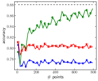
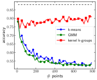
Figure 1: We report the mean accuracy (error bars are too small to be visible) over 100 Monte Carlo runs. (a) $x\sim\tfrac{1}{2}\mathcal{N}(0,1.5)+\tfrac{1}{2}\mathcal{N}(1.5,0.3)$; (b) $x\sim\tfrac{1}{2}e^{\mathcal{N}(0,1.5)}+\tfrac{1}{2}e^{\mathcal{N}(1.5,0.3)}$.

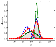
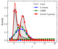
Figure 2: We consider 2000 points sampled from the same respective distributions of Fig. 1. We perform a kernel density estimation for kernel k-groups, while for k-means and GMM we show the estimated Gaussian fit. The respective accuracies for k-means, GMM, and kernel k-groups are as follows: (a) $\{0.764,0.870,0.800\}$; (b) $\{0.516,0.533,0.851\}$. Note that in the latter case only kernel k-groups was able to distinguish the two classes.

5.1.1 One-dimensional case

We first consider one-dimensional data for a two-class problem as shown in Fig. 1. Note that in Fig. 1a GMM is more accurate, as expected, however in Fig. 1b kernel k-groups outperforms both methods for non Gaussian data. GMM and k-means basically cluster at chance as $n$ increases. This illustrates the model free character of energy statistics. For these same distributions, in Fig. 2 we show a kernel density estimation and Gaussian fits. In Fig. 2b only kernel k-groups was able to distinguish between the two classes. The accuracy results are also indicated in the caption. We remark that in one dimension it is possible to simplify the formulas for energy statistics and obtain an exact deterministic algorithm, i.e. without any initialization. This is Algorithm 3 in the Appendix. We stress that kernel k-groups given by Algorithm 2 performed the same as Algorithm 3.

5.1.2 Multi-dimensional case

Next, we analyze how the algorithms degrade as dimension increases. Consider the Gaussian mixture

$$\begin{split}x&\sim\tfrac{1}{2}\mathcal{N}(\mu_{1},\Sigma_{1})+\tfrac{1}{2}\mathcal{N}(\mu_{2},\Sigma_{2}),\qquad\Sigma_{1}=\Sigma_{2}=I_{D},\\ \mu_{1}&=(\underbrace{0,\dotsc,0}_{\times D})^{\top},\qquad\mu_{2}=0.7(\underbrace{1,\dots,1}_{\times 10},\underbrace{0,\dots,0}_{\times(D-10)})^{\top}.\end{split}$$ (56)

We can compute the Bayes error which is fixed as $D$ increases, giving an optimal accuracy of $\approx 0.86$. We sample $200$ points and do 100 Monte Carlo runs. The results are in Fig. 3a. Note that kernel k-groups and spectral clustering behave similarly, being superior to the other methods. The improvement is noticeable in higher dimensions.

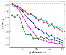
(a)

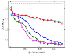
(b)

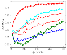
(c)

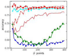
(d)

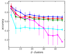
(e)

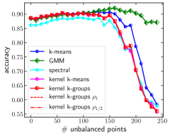
(f)

Figure 3: Comparing kernel k-groups to other methods; see legend in plot (f). For each experiment, except for (e), we perform 100 Monte Carlo runs and show the mean accuracy (error bars are standard deviation but are too small to be visible). (a) Higher dimensional Gaussian mixture (56). Dashed line is Bayes accuracy $\approx 0.86$. We use the standard energy statistics metric $\rho_{1}$ in (52). (b) Higher dimensional Gaussian mixture (57). Bayes accuracy is $\approx 0.95$. We again use $\rho_{1}$. (c) Gaussian mixture with parameters (58). We increase the number of data points, and compare different metrics (see (52)–(54)). The best results for kernel k-groups and spectral clustering use $\widetilde{\rho}_{1}$. (d) Same as in (c) but for lognormal mixture with (58). The plot suggests that neither of these methods are consistent in this case since Bayes accuracy is $\approx 0.90$. (e) Effect of large number of clusters on a two-dimensional grid. All clusters have 10 points sampled from $\mathcal{N}(\mu,0.1I)$ where $\mu$ assume coordinates on the grid (separated by one unit). We increase the number of clusters and use the standard $\rho_{1}$. (f) Unbalanced clusters. The data is normally distributed (59) where we vary $m\in[0,240]$. We use the standard metric $\rho_{1}$.

Still for the mixture (56), we now choose entries for the diagonal covariance $\Sigma_{2}$. We have $\Sigma_{1}=I_{D}$, $\mu_{1}=(0,\dotsc,0)^{\top}\in\mathbb{R}^{D}$, $\mu_{2}=(1,\dotsc,1,0,\dotsc,0)^{T}\in\mathbb{R}^{D}$, with signal in the first $10$ dimensions, and

$$\begin{split}\Sigma_{2}&=\left(\begin{array}[]{c|c}\widetilde{\Sigma}_{10}&0\\ \hline\cr 0&I_{D-10}\end{array}\right),\\ \widetilde{\Sigma}_{10}&=\operatorname{diag}(1.367,3.175,3.247,4.403,1.249,\\ &\hskip 36.0001pt1.969,4.035,4.237,2.813,3.637).\end{split}$$ (57)

We simply pick $10$ numbers at random on the range $[1,5]$ (other choice would give analogous results). Bayes accuracy is fixed at $\approx 0.95$. From Fig. 3b we see that all methods quickly degenerate as dimensions increases, except kernel k-groups and spectral clustering which are more stable.

Consider $x\sim\tfrac{1}{2}\mathcal{N}(\mu_{1},\Sigma_{1})+\tfrac{1}{2}\mathcal{N}(\mu_{2},\Sigma_{2})$ with

$$\begin{split}2\Sigma_{1}&=\Sigma_{2}=I_{20}\\ \mu_{1}&=(\underbrace{0,\dotsc,0}_{\times 20})^{\top},\quad\mu_{2}=\tfrac{1}{2}(\underbrace{1,\dotsc,1}_{5},\underbrace{0,\dotsc,0}_{15})^{\top}.\end{split}$$ (58)

Bayes accuracy is $\approx 0.90$. We now increase the sample size in the range $n\in[10,400]$. The results are in Fig. 3c. We compare kernel k-groups with different metrics, and we use the best metric, $\widetilde{\rho}_{1}$, for spectral clustering. Note the superior performance of kernel k-groups.

To consider non-Gaussian data, we sample a lognormal mixture, $x\sim(1/2)e^{\mathcal{N}(\mu_{1},\Sigma_{1})}+(1/2)e^{\mathcal{N}(\mu_{2},\Sigma_{2})}$, with the same parameters as in (58). The optimal Bayes accuracy is still $\approx 0.90$. We use exactly the same metrics as in the Gaussian mixture of Fig. 3c to illustrate that kernel k-groups still performs accurately.

To see the effect of high number of clusters, we sample 10 points from $\mathcal{N}(\mu_{\ell},0.1\,I)$ for each class, where $\mu_{\ell}$ is in a two-dimensional grid spaced by one unit. We thus increase the number of clusters $\ell\in\{2,3,\dotsc,50\}$. For each $\ell$ we perform 20 Monte Carlo runs and show the mean accuracy and the standard deviation (errorbars) in Fig. 3e. The reason spectral clustering behaves worse is due to the choice of metric (52) ($\alpha=1$). With a better choice it behaves as accurate as kernel k-groups, but we wish to illustrate the results with the standard metric from energy statistics. The important observation is that kernel k-means eventually degenerates as the number of clusters becomes too large, as opposed to kernel k-groups.

Finally, we show a limitation of kernel k-groups, which is shared among the other methods except for GMM. As we can see from Fig. 3f, for highly unbalanced clusters, k-means, spectral clustering, kernel k-means and kernel k-groups all degenerate more quickly than GMM. Here we are generating data according to

$$\begin{split}x&\stackrel{{\scriptstyle iid}}{{\sim}}\dfrac{n_{1}}{2N}\mathcal{N}(\mu_{1},\Sigma_{1})+\dfrac{n_{1}}{2N}\mathcal{N}(\mu_{1},\Sigma_{1}),\\ \mu_{1}&=(0,0,0,0)^{\top},\quad\mu_{2}=1.5\times(1,1,0,0)^{\top},\\ \Sigma_{1}&=I_{4},\quad\Sigma_{2}=\left(\begin{array}[]{c|c}\tfrac{1}{2}I_{2}&0\\ \hline\cr 0&I_{2}\end{array}\right),\\ n_{1}&=N-m,\quad n_{2}=N+m,\quad N=300.\end{split}$$ (59)

We then increase $m\in[0,240]$ making the clusters progressively more unbalanced. Based on this experiment, an interesting problem would be to extend kernel k-groups to account for unbalanced clusters.

5.2 Community detection in stochastic block models

We now illustrate the versatility of kernel k-groups on the problem of detecting communities in graphs. This problem has important applications in natural, social and computer sciences (see e.g. [35]). The classical paradigm is the stochastic block model (see [36] for a recent review) where a graph $\mathcal{G}=(\mathcal{V},\mathcal{E},\mathcal{A})$ has its vertex set partitioned into $k$ clusters, $\mathcal{V}=\mathcal{C}_{1}\cup\mathcal{C}_{2}\cup\dotsm\cup\mathcal{C}_{k}$, with each vertex $i\in\mathcal{V}$ assigned to class $C_{\ell}$, for some $\ell\in\{1,\dotsc,k\}$, with probability $\mathbb{P}[i\in\mathcal{C}_{\ell}]=1/k$. Then, conditioned on the class assignment, edges are created independently with $\mathbb{P}[\mathcal{A}_{ij}=1]=p_{\textnormal{in}}$ if $i,j\in\mathcal{C}_{\ell}$, i.e. both vertices are in the same class, and $\mathbb{P}[\mathcal{A}_{ij}=1]=p_{\textnormal{out}}$ otherwise.

We are particularly interested in sparse graphs where algorithmic challenges arise. In this case, the probabilities scale as

$$p_{\textnormal{in}}=a/n,\qquad p_{\textnormal{out}}=b/n,$$ (60)

for some constants $a,b>0$. Thus, the average degree is

$$d\equiv\mathbb{E}[d_{i}]=\left(a+(k-1)b\right)/k.$$ (61)

We assume that $\mathcal{G}$ is assortative, i.e. $a>b$. A quantity playing a distinguished role is the “signal-to-noise ratio,” denoted by $\lambda$ and defined below. A striking conjecture has been proposed [37], namely, when $n\to\infty$ there exists a detectability threshold such that unless

$$\lambda\equiv(a-b)/\sqrt{kd}>1$$ (62)

there is no polynomial time algorithm able to detect communities. Therefore, one expects that a good algorithm should be able to detect communities all the way down to the critical point $\lambda\approx 1$. Although standard spectral methods based on Laplacian or adjacency matrices work well when the graph is sufficiently dense, they are suboptimal for sparse graphs [41, 42]; in some cases failing miserably even when other methods such as belief propagation [43] and semidefinte relaxations [42] perform very well.

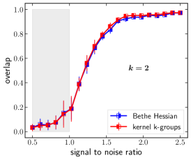
(a)

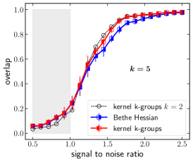
(b)

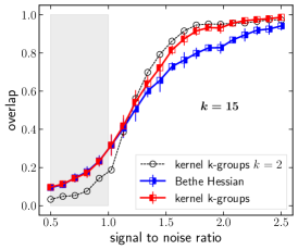
(c)

Figure 5: Comparison of kernel k-groups (Algorithm 2) to Bethe Hessian [44] (see also [42]). We choose a stochastic block model with $n=1000$ vertices and average degree $d=3$. We plot the overlap (63) against the signal-to-noise ratio (62). We sample $100$ graphs (dots are the mean and error bars one standard deviation). (a) Both methods perform closely, but with a minor improvement of kernel k-groups. (b, c) Bethe Hessian degenerates performance as $k$ increases, contrary to kernel k-groups which remains accurate; we include the result with $k=2$ (dashed black line) for reference.

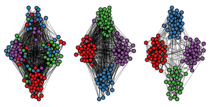
Figure 4: Girvan-Newman benchmark [45] where $n=128$, $k=4$, and $d=16$. (a) $\lambda=1.1$, (b) $\lambda=2.0$, and (c) $\lambda=3.5$. Note how the clusters become more well-defined as $\lambda>1$ increases. See Table I for clustering results.

Recently, an interesting approach based on the Bethe free energy of Ising spin models over graphs was proposed [44]. The resulting spectral method uses the Bethe Hessian matrix $\mathcal{H}_{r}\equiv(r^{2}-1)I-r\mathcal{A}+\mathcal{D}$, where $r=\sqrt{d}$ and $\mathcal{D}$ is the degree matrix of $\mathcal{G}$. Such a method achieves optimal performance for stochastic block models, being cheaper and even superior than [41] and very close to belief propagation. Hence, we now consider applying kernel k-groups (Algorithm 2) to the matrix $\mathcal{H}_{r}$, and we set the weights $\mathcal{W}=\mathcal{D}$. We wish to verify if kernel k-groups is able to perform closely to the Bethe Hessian method [44]. To this end, we initialize kernel k-groups with the output of Bethe Hessian since this allows us to check for potential improvements or not. To keep consistency with previous works, we evaluate these algorithms on the

$$\mbox{overlap}(Z,\hat{Z})\equiv\tfrac{k}{k-1}\left(\mbox{accuracy}(Z,\hat{Z})-\tfrac{1}{k}\right)$$ (63)

which simply discounts pure chance from the accuracy (55).

First, consider the classical benchmark test [45] depicted in Fig. 4. Here the average degree is $d=16$. By changing $\lambda$ one controls the within versus between class edge probability. Fig. 4 shows one realization of such graphs for three different values of $\lambda$. Note how the communities become well-defined as $\lambda$ increases away from critical point $\lambda=1$. In Table I we show clustering results for several realizations of such graphs (averaged over 500 trials). Somewhat surprisingly, kernel k-groups improves over Bethe Hessian.

TABLE I: Clustering graphs from the model shown in Fig. 4. We report the mean overlap (63) and standard deviation over 500 trials. (The case $\lambda=0.6$ is undetectable; see (62).)

$\lambda$	Bethe Hessian	kernel k-groups
$0.6$	$0.183\pm 0.058$	$0.177\pm 0.057$
$1.1$	$0.485\pm 0.123$	$\bm{0.489\pm 0.133}$
$1.5$	$0.840\pm 0.075$	$\bm{0.870\pm 0.074}$
$1.8$	$0.943\pm 0.033$	$\bm{0.960\pm 0.027}$
$2.0$	$0.975\pm 0.022$	$\bm{0.982\pm 0.020}$
$2.5$	$0.997\pm 0.006$	$\bm{0.998\pm 0.005}$
$3.5$	$1.000\pm 0.000$	$\bm{1.000\pm 0.000}$

We now approach a more challenging case to analyze the performance of kernel k-groups all the way through the phase transition (62). Consider a stochastic block model with $n=1000$ vertices and average degree $d=3$, which is much sparser than the graphs shown in Fig. 4. Thus, in Fig. 5 we plot the overlap (63) versus $\lambda$ for different number of communities. In Fig. 5a we see that kernel k-groups is very close to Bethe Hessian, although it has mild improvements. As we increase $k$, we see from Fig. 5b and Fig. 5c that Bethe Hessian degenerates performance while kernel k-groups remains stable (we include the line for the case $k=2$ as a reference). From these examples it is clear that kernel k-groups can improve over Bethe Hessian.

It is worth mentioning that kernel k-groups is even cheaper than Bethe Hessian (see Theorem 4). However, it needs a good initialization to be able to cluster with small values of $\lambda$. Here we initialized with Bethe Hessian and kernel k-groups provided a refined solution. We verified that under random or k-means++ initialization it is unable to cluster sparse graphs with small $\lambda$, although it is able to cluster cases where $\lambda$ and/or $d$ are sufficiently large.

Finally, we stress that kernel k-means cannot even be applied to this problem since $\mathcal{H}_{r}$ is not positive semidefinite. We actually tried to run the algorithm but it diverged innumerable times.

5.3 Real data experiments

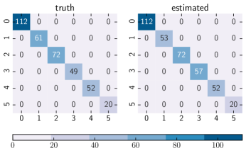
Figure 6: Clustering the dermatology dataset [46, 47] with kernel k-groups using $\rho_{1/2}$ (see (52)). We show a heatmap of the class membership. This should be compared with Table 2 of [5] (our results are more accurate). See also Table II.

We first consider the dermatology dataset [46, 47] which has 366 data points and 34 attributes, 33 being linear valued and one categorical. There are 8 data points with missing entries in the “age” column. We complete such entries with the mean of the entire column, and then we normalize the data. There are $6$ classes, and this is a challenging problem. We refer the reader to [46, 47] for a complete description of the dataset, and also to [5] where this dataset was previously analyzed. In Fig. 6 we show a heatmap of the class membership obtained with kernel k-groups using the metric (52) with $\alpha=1/2$. In Table II we compare it to other methods, and also with [5, 6]. One can see that kernel k-groups has a better performance.

TABLE II: Dermatology dataset [46, 47] (see also Fig. 6). We show accuracy (55), adjusted Rand index (aRand), and NMI. [5] obtained $\textnormal{aRand}=0.9195$, while [6] obtained $\textnormal{aRand}=0.9188$ where points with missing entries are removed. Below we complete the missing entries with the mean. If we remove points with missing entries, kernel k-groups provides an additional improvement of $\textnormal{accuracy}=0.964$, $\textnormal{aRand}=0.939$ and $\textnormal{NMI}=0.937$.

method	accuracy	aRand	NMI
kmeans	$0.738$	$0.703$	$0.860$
GMM	$0.781$	$0.737$	$0.821$
spectral clustering	$0.956$	$0.920$	$0.917$
kernel k-means	$0.872$	$0.832$	$0.879$
kernel k-groups	$\bm{0.962}$	$\bm{0.936}$	$\bm{0.932}$

Next, we consider several datasets from the public UCI repository [46] (which the reader is referred to for details). With the purpose of comparing kernel k-groups to kernel k-means and spectral clustering on equal footing, we fix the metric (53) in all cases, with $\sigma=2$. We verified that this choice in general works well for these methods in the considered datasets. We stress that we are not interested in the highest performance on individual datasets and such a choice of metric may be suboptimal for particular cases. However, by fixing the metric, each algorithm solves the same optimization problem (for a given dataset) and the comparison is fair. In our experiments, we use a single initialization and perform a total of 100 Monte Carlo runs, where kernel k-groups and kernel k-means are initialized with k-means++, while spectral clustering uses the default implementation from scikit-learn [33]. In Table III we report the mean value of NMI. To complement this table, in Fig. 7 we show violin plots where one can see the distribution of the output of each algorithm. We conclude that in most cases kernel k-groups has an improved performance, and usually a smaller variance compared to kernel k-means.

TABLE III: Kernel k-groups (groups), kernel k-means (means) and spectral clustering (spectral) on several public datasets from UCI repository [46]. We fix the metric $\tilde{\rho}_{2}$ (53). We perform 100 Monte Carlo runs and report the mean value of NMI. We complement this table by showing the distribution of these results in Fig. 7.

dataset	$n$	$k$	$D$	means	spectral	groups
libras movement	$360$	$15$	$90$	$0.535$	$\bm{0.606}$	$0.590$
vehicle	$846$	$4$	$18$	$\bm{0.166}$	$0.120$	$0.126$
forest	$523$	$4$	$27$	$\bm{0.457}$	$0.378$	$0.450$
covertype	$1400$	$7$	$54$	$\bm{0.247}$	$0.230$	$0.242$
segmentation	$210$	$7$	$19$	$0.613$	$0.597$	$\bm{0.618}$
wine	$178$	$3$	$13$	$0.867$	$0.879$	$\bm{0.928}$
synthetic control	$600$	$6$	$60$	$0.781$	$0.770$	$\bm{0.790}$
fertility	$100$	$2$	$9$	$0.019$	$0.020$	$\bm{0.021}$
glass	$214$	$6$	$9$	$0.396$	$0.377$	$\bm{0.413}$
ionosphere	$351$	$2$	$3$	$0.192$	$0.160$	$\bm{0.205}$
epileptic	$2000$	$5$	$178$	$0.222$	$0.195$	$\bm{0.251}$
anuran	$2000$	$10$	$22$	$0.622$	$0.593$	$\bm{0.635}$
gene expression	$801$	$5$	$200$	$0.554$	$0.575$	$\bm{0.637}$
pendigits	$2000$	$10$	$16$	$0.710$	$0.715$	$\bm{0.715}$
seeds	$210$	$3$	$7$	$0.720$	$0.686$	$\bm{0.748}$
spect heart	$267$	$2$	$22$	$0.163$	$0.016$	$\bm{0.180}$
iris	$150$	$3$	$4$	$0.748$	$0.742$	$\bm{0.759}$
contraceptive	$1473$	$3$	$9$	$0.036$	$0.034$	$\bm{0.037}$

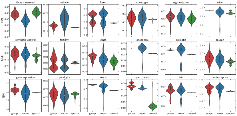
Figure 7: Violin plots showing the distribution of the results obtained in the experiments of Table III: kernel k-groups (red), kernel k-means (blue) and spectral clustering (green). We consider 100 Monte Carlo runs for each experiment. In most cases kernel k-groups has a smaller variance compared to kernel k-means (both are initialized with k-means++).

We now consider kernel k-groups applied to community detection in real world networks (we use the approach described in in Section 5.2) and compare it to the Bethe Hessian [44] and spectral clustering applied to the adjacency matrix, which in general does not work well for sparse graphs but we include as a reference and also because many real networks are not necessarily sparse. We start with four datasets that were considered extensively in the literature, for which our results are shown in Table IV. Kernel k-groups perform similarly to Bethe Hessian, but it was able to improve in one of these datasets.

TABLE IV: Community detection in real world networks with ground truth. We compare kernel k-groups to spectral clustering (on the adjacency matrix) and Bethe Hessian [44]. We report the overlap (63).

network	spectral	Bethe	k-groups
karate [48] ($k=2,d=5$)	$1.00$	$1.00$	$1.00$
dolphins [49] ($k=2,d=5$)	0.64	0.97	$\bm{1.00}$
football [45] ($k=12,d=11$)	0.90	0.90	0.90
polbooks [50] ($k=3,d=8$)	0.58	0.75	0.75

We now consider networks without ground truth. We use three standard metrics in graph clustering: performance, coverage, and modularity. (We refer to [51] for details.) These metrics are always in the range $[0,1]$ with larger values indicating better defined communities. We consider the network obtained from both hemispheres of a drosophila brain [52]. The data is separated into left and right parts. It is also heavily connected, e.g. the left graph has 209 nodes and the right graph has 213 nodes, and for both the average degree is $d\approx 53$. Thus we do not expect the modularity to be a good measure of clustering in this setting. The number of clusters was found by computing the number of negative eigenvalues of the matrix $\mathcal{H}_{r}$ (see Section 5.2) [44]. For both graphs we found that $k=2$. Our results are reported in Table V and an illustration of the clustered graph with kernel k-groups is in Fig. 8a. Note that kernel k-groups had better scores than competitor methods.

TABLE V: Clustering the drosophila connectome [52]. Left: $|\mathcal{V}|=209$, $|\mathcal{E}|=11118$, $d=53$. We found $k=2$ and the number of nodes in each community are $\{116,93\}$. Right: $|\mathcal{V}|=213$, $|\mathcal{E}|=11250$, $d=53$. The number of nodes in each community are $\{112,101\}$. Kernel k-groups improve over the other methods according to performance and coverage. For an illustration see Fig. 8a.

drosophila	method	performance	coverage	modularity
left	spectral	$0.43$	$0.65$	$0.074$
	Bethe	$0.48$	$0.71$	$0.082$
	k-groups	$\bm{0.67}$	$\bm{0.84}$	$0.041$
right	spectral	$0.43$	$0.71$	$0.074$
	Bethe	$0.44$	$0.81$	$0.071$
	k-groups	$\bm{0.66}$	$\bm{0.83}$	$0.055$

Next we consider the arXiv GR-QC dataset [53] which contains a network of scientific collaborations in General Relativity and Quantum Cosmology during a period of 10 years (from Jan 1993 to Jan 2003). Our results are shown in Table VI. We found $k=165$ for this network from the negative eigenvalues of $\mathcal{H}_{r}$. Note from Table VI that kernel k-groups improves over the Bethe Hessian according to the three metrics. An illustration of the graph grouped into communities is shown in Fig. 8b. We see that there is a large community (purple) followed by several other smaller ones.

TABLE VI: Community detection in arXiv GR-QC network [53]. This graph has $|\mathcal{V}|=5242$, $|\mathcal{E}|=14496$, with average degree $d\approx 5.5$. Kernel k-groups achieves higher scores for the three metrics compared to the alternative methods.

method	performance	coverage	modularity
spectral	$0.63$	$0.57$	$0.49$
Bethe	$0.78$	$0.71$	$0.46$
k-groups	$\bm{0.86}$	$\bm{0.81}$	$\bm{0.55}$

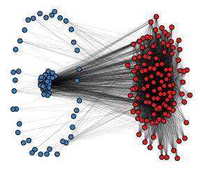
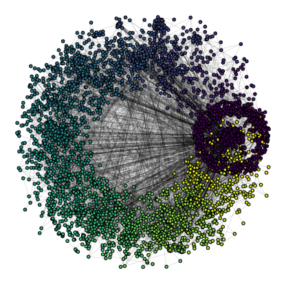
Figure 8: (a) Drosophila left hemisphere [52] after clustered into $k=2$ communities with kernel k-groups (see Table V). A very similar picture is obtained for the right hemisphere, and thus omitted. For the left hemisphere one class has $116$ nodes and the other $93$. For the right hemisphere one class has $112$ nodes and the other $101$. (b) Graph obtained after clustering the arXiv GR-QC network [53] (see Table VI). Note that there is a large community (purple) that is highly connected, and many other smaller communities. The number of nodes in the top 5 communities are $\{1955,200,123,101,79,\dotsc\}$.

6 Conclusion

On the theoretical side, we proposed a formulation to clustering based on energy statistics, valid for arbitrary spaces of negative type. Such a mathematical construction reduces to a QCQP in the associated RKHS, as demonstrated in Proposition 2. We showed that the optimization problem is equivalent to kernel k-means, once the kernel is fixed, and also to several graph partitioning problems.

On the algorithmic side, we extended Hartigan’s method to kernel spaces and proposed Algorithm 2, which we called kernel k-groups. This method was compared to kernel k-means and spectral clustering algorithms, besides k-means and GMM. Our numerical results show a superior performance of kernel k-groups, which is notable in higher dimensions. We stress that kernel k-groups has the same complexity of kernel k-means algorithm, $\mathcal{O}(n^{2})$, which an order of magnitude lower than spectral clustering, $\mathcal{O}(n^{3})$.

We illustrated the advantages of kernel k-groups when applied to community detection in sparse graphs sampled from the stochastic block model, which has several important applications ranging from physical, computer, biological, and social sciences. We thus expect that kernel k-groups may find wide applicability. We also tested the proposed method in several real world datasets, and in the vast majority of cases it improved over the alternatives.

Kernel k-groups suffers a limitation, also shared by kernel k-means and spectral clustering, which involves highly unbalanced clusters. An interesting problem that we leave open is to extend the method to such situations. Finally, kernel methods can greatly benefit from sparsity and fixed-rank approximations of the Gram matrix and there is plenty of room to make kernel k-groups scalable to large data.

References

- [1] G. J. Székely and M. L. Rizzo. Energy Statistics: A Class of Statistics Based on Distances. Journal of Statistical Planning and Inference, 143:1249–1272, 2013.
- [2] G. J. Székely and M. L. Rizzo. The Energy of Data. Annu. Rev. Stat. Appl., 207:447–479, 2017.
- [3] M. L. Rizzo and G. J. Székely. DISCO Analysis: A Nonparametric Extension of Analysis of Variance. The Annals of Applied Statistics, 4(2):1034–1055, 2010.
- [4] G. J. Székely, M. L. Rizzo, and N. K. Bakirov. Measuring and testing dependence by correlation of distances. Ann. Stat., 35(6):2769–2794, 2007.
- [5] G. J. Székely and M. L. Rizzo. Hierarchical Clustering via Joint Between-Within Distances: Extending Ward’s Minimum Variance Method. Journal of Classification, 22(2):151–183, 2005.
- [6] S. Li and M. Rizzo. -Groups: A Generalization of -Means Clustering. arXiv:1711.04359 [stat.ME], 2017.
- [7] R. Lyons. Distance Covariance in Metric Spaces. The Annals of Probability, 41(5):3284–3305, 2013.
- [8] D. Sejdinovic, B. Sriperumbudur, A. Gretton, and K. Fukumizu. Equivalence of Distance-Based and RKHS-Based Statistic in Hypothesis Testing. The Annals of Statistics, 41(5):2263–2291, 2013.
- [9] C. Shen and J. T. Vogelstein. The exact equivalence of distance and kernel methods for hypothesis testing. arXiv:1806.05514 [stat.ML], 2018.
- [10] S. P. Lloyd. Least Squares Quantization in PCM. IEEE Transactions on Information Theory, 28(2):129–137, 1982.
- [11] J. B. MacQueen. Some Methods for Classification and Analysis of Multivariate Observations. In Proceedings of the 5th Berkeley Symposium on Mathematical Statistics and Probability, volume 1, pages 281–297. University of California Press, 1967.
- [12] E. Forgy. Cluster Analysis of Multivariate Data: Efficiency versus Interpretabiliby of Classification. Biometrics, 21(3):768–769, 1965.
- [13] B. Schölkopf, A. J. Smola, and K. R. Müller. Nonlinear Component Analysis as a Kernel Eigenvalue Problem. Neural Computation, 10:1299–1319, 1998.
- [14] M. Girolami. Kernel Based Clustering in Feature Space. Neural Networks, 13(3):780–784, 2002.
- [15] J. Mercer. Functions of Positive and Negative Type and their Connection with the Theory of Integral Equations. Proceedings of the Royal Society of London, 209:415–446, 1909.
- [16] I. S. Dhillon, Y. Guan, and B. Kulis. Kernel K-means: Spectral Clustering and Normalized Cuts. In Proceedings of the Tenth ACM SIGKDD International Conference on Knowledge Discovery and Data Mining, KDD ’04, pages 551–556, New York, NY, USA, 2004. ACM.
- [17] I. S. Dhillon, Y. Guan, and B. Kulis. Weighted Graph Cuts without Eigenvectors: A Multilevel Approach. IEEE Transactions on Pattern Analysis and Machine Intelligence, 29(11):1944–1957, 2007.
- [18] M. Filippone, F. Camastra, F. Masulli, and S. Rovetta. A Survey of Kernel and Spectral Methods for Clustering. Pattern Recognition, 41:176–190, 2008.
- [19] J. A. Hartigan. Clustering Algorithms. John Wiley & Sons, Inc., New York, NY, USA, 1975.
- [20] J. A. Hartigan and M. A. Wong. Algorithm AS 136: A -Means Clustering Algorithm. Journal of the Royal Statistical Society. Series C (Applied Statistics), 28(1):100–108, 1979.
- [21] M. Telgarsky and A. Vattani. Hartigan’s Method: -Means Clustering without Voronoi. In Proceedings of the 13th International Conference on Artificial Intelligence and Statistics (AISTATS), volume 9, pages 313–319. JMLR, 2010.
- [22] N. Slonim, E. Aharoni, and K. Crammer. Hartigan’s -Means versus Lloyd’s -Means — Is it Time for a Change? In Proceedings of the 20th International Conference on Artificial Intelligence, pages 1677–1684. AAI Press, 2013.
- [23] N. Aronszajn. Theory of Reproducing Kernels. Transactions of the American Mathematical Society, 68(3):337–404, 1950.
- [24] A. Gretton, K. M. Borgwardt, M. J. Rasch, B. Schölkopf, and A. Smola. A Kernel Two-Sample Test. Journal of Machine Learning Research, 13:723–773, 2012.
- [25] L. Song, A. Smola, A. Gretton, and K. Borgwardt. A dependence maximization view of clustering. ICML, 2007.
- [26] C. Berg, J. P. R. Christensen, and P. Ressel. Harmonic Analysis on Semigroups: Theory of Positive Definite and Related Functions. Graduate Text in Mathematics 100. Springer, New York, 1984.
- [27] J. Shi and J. Malik. Normalized Cust and Image Segmentation. IEEE Transactions on Pattern Analysis and Machine Intelligence, 22(8):888–905, 2000.
- [28] A. Y. Ng, M. I. Jordan, and Y. Weiss. On Spectral Clustering: Analysis and an Algorithm. In Advances in Neural Information Processing Systems, volume 14, pages 849–856, Cambridge, MA, 2001. MIT Press.
- [29] D. Niu, J. G. Dy, and M. I. Jordan. Dimensionality reduction for spectral clustering. AISTATS, 2011.
- [30] B. Kernighan and S. Lin. An Efficient Heuristic Procedure for Partitioning Graphs. The Bell System Technical Journal, 49(2):291–307, 1970.
- [31] P. Chan, M. Schlag, and J. Zien. Spectral -Way Ratio Cut Partitioning. IEEE Transactions on Computer-Aided Design of Integrated Circuits and Systems, 13:1088–1096, 1994.
- [32] S. X. Yu and J. Shi. Multiclass Spectral Clustering. In Proceedings Ninth IEEE International Conference on Computer Vision, volume 1, pages 313–319, 2003.
- [33] F. Pedregosa, G. Varoquaux, A. Gramfort, V. Michel, B. Thirion, O. Grisel, M. Blondel, P. Prettenhofer, R. Weiss, V. Dubourg, J. Vanderplas, A. Passos, D. Cournapeau, M. Brucher, M. Perrot, and E. Duchesnay. Scikit-learn: Machine learning in Python. Journal of Machine Learning Research, 12:2825–2830, 2011.
- [34] D. Arthur and S. Vassilvitskii. -means++: The Advantage of Careful Seeding. In Proceedings of the Eighteenth annual ACM-SIAM Symposium on Discrete Algorithms, pages 1027–1035, Philadelphia, PA, USA, 2007. Society for Industrial and Applied Mathematics.
- [35] S. Fortunato and D. Hric. Community Detection in Networks: A User guide. Physics Reports, 659:1–44, 2016.
- [36] E. Abbe. Community Detection and Stochastic Block Models: Recent Developments. Journal of Machine Learning Research, 18:1–86, 2018.
- [37] A. Decelle, F. Krzakala, C. Moore, and L. Zdeborová. Asymptotic Analysis of the Stochastic Block Model for Modular Networks and its Algorithmic Applications. Phys. Rev. E, 86:066106, 2011.
- [38] L. Massoulié. Community Detection Thresholds and the Weak Ramanujan Property. In Proceedings of the Forty-sixth Annual ACM Symposium on Theory of Computing, STOC ’14, pages 694–703, 2014.
- [39] E. Mossel, J. Neeman, and A. Sly. ”a proof of the block model threshold conjecture”. Combinatorica, 38(3):665–708, 2018.
- [40] E. Abbe and C. Sandon. Proof of the Achievability Conjectures for the General Stochastic Block Model. Comm. Pure and Applied Math., LXXI:1334–1406, 2018.
- [41] F. Krzakala, C. Moore, E. Mossel, J. Neeman, A. Sly, and L. Zdeborová. Spectral Redemption in Clustering Sparse Networks. Proc. Nat. Acad. Sci., 110(52):20935––20940, 2013.
- [42] A. Javanmard, A. Montanari, and F. Ricci-Tersenghi. Phase transitions in semidefinite relaxations. Proc. Nat. Acad. Sci., 113(16):E2218–E2223, 2016.
- [43] Y. Watanabe and K. Fukumizu. Graph Zeta Function in the Bethe Free Energy and Loopy Belief Propagation. pages 2017–2025, 2009.
- [44] A. Saade, F. Krzakala, and L. Zdeborová. Spectral Clustering of Graphs with the Bethe Hessian. Proc. Int. Conf. Neural Information Processing Systems, 2014.
- [45] M Girvan and M. E. J. Newman. Community Structure in Social and Biological Networks. Proc. Nat. Acad. Sci., 99(12):7821–7826, 2002.
- [46] D. Dua and C. Graff. UCI machine learning repository, 2017. University of California, Irvine, School of Information and Computer Sciences, http://archive.ics.uci.edu/ml.
- [47] H. A. Güvenir, G. Demiröza, and N. Ilterb. Learning differential diagnosis of erythemato-squamous diseases using voting feature intervals. Artificial Intelligence in Medicine, 13(3):147–165, 1998.
- [48] W. W. Zachary. An Information Flow Model for Conflict and Fission in Small Groups. J. Anthropological Research, 33:452–473, 1977.
- [49] D. Lusseau, K. Schneider, O. J. Boisseau, P. Haase, E. Slooten, and S. M. Dawson. The Bottlenose Dolphin Community of Doubtful Sound Features a Large Proportion of Long-Lasting Associations. Behavioral Ecology and Sociobiology, 54:396–405, 2003.
- [50] V. Krebs.
- [51] S. Fortunato. Community Detection in Graphs. Physics Reports, 486:75–174, 2010.
- [52] K. Eichler, F. Li, A. Litwin-Kumar, Y. Park, I. Andrade, C. M. Schneider-Mizell, T. Saumweber, A. Huser, C. Eschbach, B. Gerber, R. D. Fetter, J. W. Truman, C. E. Priebe, L. F. Abbott, A. S. Thum, M. Zlatic, and A. Cardona. The Complete Connectome of a Learning and Memory Centre in an Insect Brain. Nature, 548:175 EP–, 2017.
- [53] J. Leskovec, J. Kleinberg, and C. Faloutsos. Graph Evolution: Densification and Shrinking Diameters. ACM Trans. Know. Discov. Data, 1:396–405, 2007.
- [54] M. Rizzo and G. Szekely. energy: E-Statistics: Multivariate Inference via the Energy of Data. R package version 1.7-5; https://CRAN.R-project.org/package=energy, 2018.