Position measurement and the Huygens-Fresnel principle: A quantum model of Fraunhofer diffraction for polarized pure states

Abstract

In most theories of diffraction by a diaphragm, the amplitude of the diffracted wave, and hence the position wave function of the associated particle, is calculated directly without prior calculation of the quantum state. Few models express the state of the particle to then deduce the position and momentum wave functions related to the diffracted wave. We present a model of this type for Fraunhofer diffraction. The diaphragm is assumed to be a device for measuring the three spatial coordinates of the particles passing through the aperture. A matrix similar to the S-matrix of the scattering theory describes the process which turns out to be more complex than a simple position measurement. Some predictions can be tested. The wavelet emission involved in the Huygens-Fresnel principle occurs from several neighboring wavefronts instead of just one, causing typical damping of the diffracted wave intensity. An angular factor plausibly accounts for the decrease in intensity at large diffraction angles, unlike the obliquity factors of the wave optics theories. The position measurement modifies the polarization states and for an incident photon in an elliptically polarized pure state, the ellipse axes can undergo a rotation which depends on the diffraction angles.

Keywords: position measurement, Huygens-Fresnel principle, Fraunhofer diffraction, S-matrix, large diffraction angles, diffracted light polarization

I Introduction

Quantum mechanics is involved in many studies on diffraction. Since the first quantum theory of Fraunhofer diffraction by a grating [2], several models have emerged, using the formalism of path integrals [3, 4, 5], the calculation of trajectories in the framework of hidden variable theories [6, 7] or the resolution of the wave equation combined with the use of the Kirchhoff integral [8]. In more recent studies, various topics are discussed such as the effects of diffraction on the transmission of information in quantum optical systems [9], the role of the quantum behavior of the diaphragm electrons in diffraction of light by a small hole [10], the interactions between the quantum states of different modes in diffracted Gaussian beams [11], the connection between orbital angular momentum transfer and helicity in the diffraction of light [12].

However, one question does not seem to have received much attention: the possibility of starting from the postulates of quantum mechanics to treat diffraction by a diaphragm as a consequence of a measurement of the position of the particle associated with the wave as it passes through the aperture. The first model based on this approach relates to the measurement of one transverse coordinate and provides the same predictions as those of wave optics for the case of Fraunhofer diffraction with slits [13]. Afterward, several aspects of this model were discussed [14]. More recently, quantum trajectories has been used to describe the motion of the particle after the measurement of one transverse coordinate in a model giving predictions for Fraunhofer and Fresnel diffractions by a slit [15]. There does not seem to have been any other publications on this issue so far.

In the model presented below, we start from the observation that the detection of a particle in the far field region beyond a diaphragm provides a measurement of its momentum. Then, we assume that the distribution of this momentum results from a measurement of the three spatial coordinates of the particle during its passage through the aperture and that this position measurement has an effect on the polarization if the particle has spin. The change in momentum and polarization is described by a ”diffraction matrix” similar to the S-matrix of the scattering theory [16]. Although this model only applies to the far field, it nevertheless provides specific predictions about the Huygens-Fresnel principle, the diffraction at large angles and, in the case of light, the polarization of the photons detected beyond the diaphragm.

We present the model in Sec.  II. Next, some predictions regarding intensity and polarization measurements are described in Sec.  III. Finally, we summarize in Sec.  IV.

II Quantum model of Fraunhofer diffraction by an aperture

II.1 Measurement of quantities related to the detected particles.

II.1.1 Experimental setup and first assumptions.

The model applies for an experimental setup with the following characteristics (Fig. ​​ 1). The diaphragm is a plane assumed to be of zero thickness and perfectly opaque. The aperture, of finite area, can be of any shape and possibly formed of several parts. The origin of the laboratory frame of reference $(O;x,y,z)$ is located at the aperture and the $(Ox,Oy)$ plane is that of the diaphragm. The source is located on the $z$ axis. Detectors placed beyond the diaphragm measure the local counting rate and possibly the polarization. The position of a detection point is denoted by its radius-vector $\mathbf{d}$.

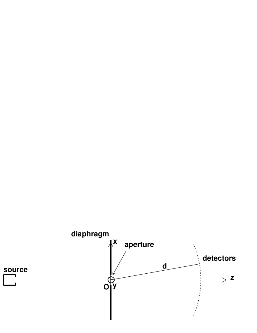
Figure 1: Experimental setup and laboratory frame of reference (right-handed coordinate system).

It is assumed that there is neither creation nor annihilation of particles during the passage of the wave through the aperture. It is also assumed that the particles are free when they move between the source and the diaphragm and between the diaphragm and the detectors. Moreover, we consider the case of a low intensity source emitting either non-relativistic particles or photons. We can then individually assign a quantum state to each non-relativistic particle or a one-photon state of the electromagnetic field to each photon, both for the incident wave and for the diffracted wave.

Finally, we suppose that the source-diaphragm and diaphragm-detector distances are large enough for the aperture to be viewed as a point from the detectors and for the incident wave to be close to a plane wave when it arrives at the aperture. For simplicity, this plane wave is supposed to be monochromatic with the wave vector $\mathbf{k}_{0}$ in the direction of the $z$ axis.

II.1.2 Measurement of the momentum of the detected particles.

From the above assumptions and conditions, we can assign the momentum $\hbar\mathbf{k}_{0}$ to the incident particle and a momentum $\hbar\mathbf{k}$ such that:

$$\mathbf{k}\;=\;\frac{k}{d}\;\mathbf{d}$$ (1)

to the particle detected at point of radius-vector $\mathbf{d}$, provided that the modulus $k$ is measured. However, no significant difference between the wavelength of the diffracted wave and that of the incident wave is observed in diffraction experiments with a diaphragm. Hence:

$$k\,\simeq\,k_{0},$$ (2)

which is in accordance with kinematics because the particle transfers a very small part of its energy to the diaphragm. So it is not required to determine $k$ by a special measurement. Furthermore, the part of the diffracted wave returning from the aperture to the region where the source is located is very weak. For simplicity, we assume that the momentum of the particle associated with the diffracted wave is always such that:

$${k_{z}}\,>\,0.$$ (3)

The relations (​​ 1), (​​ 2) and (​​ 3) imply that it is possible to measure the momentum probability density function (PDF) of the particle after its passage through the aperture in the case of diffraction at infinity. The measurement can be performed, for example, by arranging detectors on a hemisphere of center $O$ and radius $d$ in the half-space $z>0$. The radius must be such that $\Delta\ll d$, where $\Delta$ is the size of the aperture, otherwise (​​ 1) cannot be used. The Fraunhofer diffraction criterion, that is: $\Delta^{2}/(\lambda d)\,\ll\,1$ [17, 18, 19], is then satisfied if $d$ is large enough, whatever the value of $\lambda/\Delta$.

II.1.3 Measurement of the polarization of the detected particles.

The polarization measuring device (analyzer for photons, Stern and Gerlach apparatus for atoms, etc…) is placed in front of the detector which is located, given (​​ 1), in the direction of the momentum $\hbar\mathbf{k}$ of the detected particle. The measurement therefore gives the probabilities of the eigenvalues of the spin component on a quantization axis $Z[\mathbf{k}]$ which must be chosen with respect to a coordinate system $\{x[\mathbf{k}],y[\mathbf{k}],z[\mathbf{k}]\}$ attached to the detected particle. Finally, it is possible to measure, on a particle of spin ${s}$, the probability of finding the result $\sigma$ for its spin component on a $Z[\mathbf{k}]$ axis if the measurement of its momentum gives the result $\hbar\mathbf{k}$. It is therefore a conditional probability.

By convention, the coordinate system attached to the incident particle is the laboratory frame of reference (Fig. ​​ 1) whose $z\equiv z[\mathbf{k}_{0}]$ axis is in the direction of the momentum $\hbar\mathbf{k}_{0}$. For the detected particle, we choose the coordinate system obtained from the laboratory frame of reference by the rotation $\mathcal{R}(\phi,\theta,0)$ where the Euler angles are defined according to the $z-y-z$ convention, so that $\phi$ and $\theta$ are the azimuth and the polar angle, respectively, of $\mathbf{k}$. Hence:

$$l[\mathbf{k}]=\mathcal{R}(\phi,\theta,0)\,l[\mathbf{k}_{0}]\,,\hskip 7.11317ptl=x,y,z;\hskip 14.22636ptz[\mathbf{k}]\parallel\mathbf{k}.\hskip 21.33955pt$$ (4)

The zero value of the third Euler angle defines a choice of the directions of the $x[\mathbf{k}]$ and $y[\mathbf{k}]$ axes in the transverse plane to $\mathbf{k}$ such that the coordinate system attached to the detected particle in the case $\phi=\theta=0$ is coincident with the laboratory frame of reference.

Two very different cases arise concerning the quantization axis. For a non-relativistic particle, this axis can be chosen in any direction. There is then an infinite number of possible $Z[\mathbf{k}]$ axes for each vector $\mathbf{k}$. On the other hand, for a relativistic particle, the quantization axis must be in the direction of the momentum because the only spin component eigenstates are the helicity states [16]. There is then only one possibility which is $Z[\mathbf{k}]=z[\mathbf{k}]$, according to the above convention.

II.2 Diffraction operator.

II.2.1 Measurement of the position of the incident particles.

Since it is possible to measure the momentum PDF and the polarization of the particles associated with the diffracted wave at infinity, we can consider the construction of a quantum model whose purpose is to provide the expressions of these quantities. The model proposed here is based on the assumption that each incident particle undergoes a position measurement as it passes through the aperture. The detection of a particle beyond the diaphragm can indeed be considered as proof that it effectively passed through the aperture and was therefore localized at this place during a short period of time with a precision of the order of the size of the aperture [20]. For simplicity, we consider that the localization occurs instantaneously. We then assume that the source emits a particle at time $t_{0}$, that this particle passes through the aperture at time $t_{1}$ and that it is detected at time $t_{2}$. The time $t_{1}$ can then be interpreted as the time when the state of the particle changes because of the position measurement performed by the diaphragm and the purpose of the model is to build a diffraction operator which describes this change of state.

II.2.2 Using S-matrix theory formalism.

The quantum state of the particle of spin ${s}$ at time $t$ is assumed to be a pure state denoted $\left|\,\psi^{({s})}(t)\;\right>\,$. Since the incident wave is close to a monochromatic plane wave with wave vector $\mathbf{k}_{0}$ and given (​​ 2), the incident particle and the particle associated with the diffracted wave are in an energy state close to the eigenstate of eigenvalue $\hbar{\omega}_{0}$, where ${\omega}_{0}=c\,(\,\hbar^{-2}m^{2}c^{2}+{k_{0}}^{2}\,)^{1/2}$. The initial and final states are therefore close to stationary states of the form:

$$\!\!\begin{array}[]{rlcl}\displaystyle\left|\,\psi_{\textup{in}}^{({s})}(t)\!\;\right>\,\!\!&=&\exp(-\mathrm{i}{\omega}_{0}t)\,\left|\,\varphi^{({s})}_{\textup{in}}\;\right>\,\!\!,&\;\,t_{0}<t<t_{1},\vspace{0.2cm}\\ \displaystyle\left|\,\psi_{\textup{out}}^{({s})}(t)\!\;\right>\,\!\!&=&\exp(-\mathrm{i}{\omega}_{0}t)\,\left|\,\varphi^{({s})}_{\textup{out}}\;\right>\,\!\!,&\;\,t_{1}<t<t_{2}.\end{array}\hskip 15.6491pt$$ (7)

where $\left|\,\varphi^{({s})}_{\textup{in}}\;\right>\,$ and $\left|\,\varphi^{({s})}_{\textup{out}}\;\right>\,$ are time-independent states. Since time dependence only appears in global phase factors, knowing the exact values of $t_{0}$, $t_{1}$ and $t_{2}$ is not essential and, as in the S-matrix theory, we consider a diffraction operator $\hat{\mathrm{D}}^{({s})}$ which projects the initial time-independent state on the final time-independent state (called ”initial state” and ”final state” in the following). The change of state is expressed by:

$$\left|\,\varphi^{({s})}_{\textup{out}}\;\right>\,=\left[\,{N}^{({s})}\,\right]^{-1/2}\;\hat{\mathrm{D}}^{({s})}\left|\,\varphi^{({s})}_{\textup{in}}\;\right>\,,$$ (8)

where ${N}^{({s})}$ is the normalization factor:

$${N}^{({s})}\equiv\,\left<\,\varphi^{({s})}_{\textup{in}}\,\left|\left.\hat{\mathrm{D}}^{({s})}{}^{{}^{\textrm{\scriptsize$\dagger$}}}\,\hat{\mathrm{D}}^{({s})}\,\right|\,\varphi^{({s})}_{\textup{in}}\right.\right>\,.$$ (9)

All the information on the ”particle-diaphragm interaction” is contained in the matrix elements of the diffraction operator from which we can get the transition amplitudes between the initial state and the final momentum and spin component eigenstates. Since we only consider one-particle states, these eigenstates are represented by the state vectors:

$$\begin{array}[]{rlll}\hat{a}^{\dagger}(\mathbf{k})\left|\,\!\textup{vac}\!\;\right>&\!\!=\!\!&\left|\,\mathbf{k}\;\right>\,,&{s}=0,\vspace{0.2cm}\\ \hat{a}^{\dagger}\!\left(\mathbf{k},[\sigma]_{Z[\mathbf{k}]}\right)\left|\,\!\textup{vac}\!\;\right>&\!\!=\!\!&\left|\,\mathbf{k}\;\right>\,\!\!\,\otimes\,\!\left|\,\sigma\;\right>\,_{\!\!Z[\mathbf{k}]},&{s}\neq 0.\end{array}\hskip 21.33955pt$$ (12)

where $\left|\,\!\textup{vac}\!\;\right>\,$ is the vacuum state, $\hat{a}^{\dagger}\!\left(\mathbf{k},[\sigma]_{Z[\mathbf{k}]}\right)$ is the creation operator of a particle of momentum $\hbar\mathbf{k}$ and spin component $\sigma$ on the quantization axis $Z[\mathbf{k}]$ and $\left|\,\sigma\;\right>\,_{\!\!Z[\mathbf{k}]}$ is the eigenstate of spin component $\sigma$ on $Z[\mathbf{k}]$. The initial state is given by:

$$\left|\,\varphi^{({s})}_{\textup{in}}\;\right>\,=\left\{\begin{array}[]{lll}\displaystyle\left|\,\mathbf{k}_{0}\;\right>&\hskip 14.22636pt\mbox{if}&{s}=0\vspace{0.1cm}\\ \displaystyle\left|\,\mathbf{k}_{0}\;\right>\,\!\,\otimes\,\!\left|\,\chi^{({s})}_{\textup{in}}\;\right>&\hskip 14.22636pt\mbox{if}&{s}\neq 0,\end{array}\right.\hskip 21.33955pt$$ (15)

where $\left|\,\chi^{({s})}_{\textup{in}}\;\right>\,$ is the initial state of spin polarization prepared with the amplitudes ${}_{Z[\mathbf{k}_{0}]\!\!\!}\,\left<\,\sigma\left|\,\chi^{({s})}_{\textup{in}}\right.\right>\,$.

II.2.3 Structure of the diffraction operator.

From (​​ 8) and (​​ 15), the non-normalized final state for a particle without spin is expressed by:

$$\hat{\mathrm{D}}^{(0)}\!\left|\,\varphi^{(0)}_{\textup{in}}\;\right>\,\!\!=\hat{\mathrm{D}}^{(0)}\!\left|\,\mathbf{k}_{0}\;\right>\,\!\!=\!\!\int\!\mathrm{d}^{3}k\,\left|\,\mathbf{k}\;\right>\,\!\!\,\left<\,\!\mathbf{k}\!\,\left|\left.\hat{\mathrm{D}}^{(0)}\,\right|\,\!\mathbf{k}_{0}\!\right.\right>\,\!\!.\hskip 21.33955pt$$ (16)

To generalize this expression to the case of a particle of non-zero spin, we rely on the following observation. For the photon, the quantization axis is in the direction of the momentum and the eigenvalue zero of the spin component is impossible [16]. Therefore, the change in the direction of the momentum of the photon due to diffraction causes a modification of its spin polarization so that this impossibility of the eigenvalue zero is preserved. More generally, we assume that for any particle, the momentum exchange with the diaphragm causes a specific change in spin polarization.

The change in polarization corresponds to a rearrangement of the spin component wave functions and therefore results from the action of a unitary rotation operator. So we are led to assume that if the measurement of the momentum of the detected particle gives the result $\hbar\mathbf{k}$ then the probabilities of the results of a simultaneous measurement of the spin component correspond to a polarization state which depends on $\mathbf{k}$ in the form:

$$\left|\,\chi^{({s})}_{\textup{out}}(\mathbf{k})\;\right>\,=\hat{\mathrm{R}}^{({s})}[\,\alpha_{1}(\mathbf{k}),\alpha_{2}(\mathbf{k}),\alpha_{3}(\mathbf{k})\,]\,\left|\,\chi^{({s})}_{\textup{in}}\;\right>\,\!,\hskip 21.33955pt$$ (17)

where $\hat{\mathrm{R}}^{({s})}[\,\alpha_{1}(\mathbf{k}),\alpha_{2}(\mathbf{k}),\alpha_{3}(\mathbf{k})\,]$ is the operator of the spin rotation associated with the momentum transfer $\hbar\mathbf{k}_{0}\rightarrow\hbar\mathbf{k}$. The state $\left|\,\chi^{({s})}_{\textup{out}}(\mathbf{k})\;\right>\,$ is in some way the ”conditional state” of polarization associated with the momentum eigenstate $\left|\,\mathbf{k}\;\right>\,$. The Euler angles $\alpha_{j}(\mathbf{k})$ are defined with respect to the quantization axis $Z[\mathbf{k}_{0}]$ and are three parameters of the model. They are functions of $\mathbf{k}$, not known a priori. They also depend on $\mathbf{k}_{0}$ and possibly on other parameters as for example the spin of the particle: $\alpha_{j}(\mathbf{k})\equiv\alpha_{j}^{\mathbf{k}_{0},{s},...}(\mathbf{k})$.

An additional assumption is needed to generalize (​​ 16). For a spinless particle, the position and momentum wave functions are Fourier transforms of each other. In the case of diffraction with a diaphragm, the shape of the final momentum distribution is therefore determined by the shape of the aperture. We assume that this determination is the same if the particle has spin, so that the final momentum distribution of a particle with spin is the same as that of a spinless particle that would have the same energy. There do not seem to be any experimental facts invalidating this assumption.

The easiest way to generalize (​​ 16) taking into account (​​ 15), (​​ 17) and the additional assumption above is to express the action of $\hat{\mathrm{D}}^{({s})}$ on the initial state in the following form (we use the notation $\hat{\mathrm{R}}^{({s})}(\mathbf{k})$ instead of $\hat{\mathrm{R}}^{({s})}[\,\alpha_{1}(\mathbf{k}),\alpha_{2}(\mathbf{k}),\alpha_{3}(\mathbf{k})\,]$ for simplicity and we insert the identity operator $\sum_{\sigma}\left|\,\sigma\;\right>\,_{\!\!Z[\mathbf{k}]}\;{}_{\;Z[\mathbf{k}]}\!\!\,\left<\,\sigma\,\right|$):

$$\begin{array}[]{l}\displaystyle\hat{\mathrm{D}}^{({s})}\left|\,\varphi^{({s})}_{\textup{in}}\;\right>\,=\;\hat{\mathrm{D}}^{({s})}\left(\,\left|\,\mathbf{k}_{0}\;\right>\,\!\!\,\otimes\,\!\left|\,\chi^{({s})}_{\textup{in}}\;\right>\,\right)\vspace{0.2cm}\\ \displaystyle\hskip 9.95863pt=\!\int\!\mathrm{d}^{3}k\left|\,\mathbf{k}\;\right>\,\!\,\left<\,\mathbf{k}\,\left|\left.\hat{\mathrm{D}}^{(0)}\,\right|\,\mathbf{k}_{0}\right.\right>\,\!\,\otimes\,\!\left|\,\chi^{({s})}_{\textup{out}}(\mathbf{k})\;\right>\vspace{0.2cm}\\ \displaystyle\hskip 9.95863pt=\!\int\!\mathrm{d}^{3}k\left|\,\mathbf{k}\;\right>\,\!\,\left<\,\mathbf{k}\,\left|\left.\hat{\mathrm{D}}^{(0)}\,\right|\,\mathbf{k}_{0}\right.\right>\\ \displaystyle\hskip 21.33955pt\,\otimes\,\sum_{\sigma}\left|\,\sigma\;\right>\,_{\!\!Z[\mathbf{k}]}\;{}_{\;Z[\mathbf{k}]}\!\!\,\left<\,\sigma\,\left|\left.\hat{\mathrm{R}}^{({s})}(\mathbf{k})\,\right|\,\chi^{({s})}_{\textup{in}}\!\right.\right>\,\!\!,\;\;\;\;{s}\neq 0.\end{array}\hskip 21.33955pt$$ (22)

From (​​ 8), (​​ 15), (​​ 16) and (​​ 22), the final state is a linear combination of the momentum and spin component eigenstates given by (​​ 12) and the diffraction operator is:

$$\!\hat{\mathrm{D}}^{({s})}=\left\{\begin{array}[]{cl}\displaystyle\hat{\mathrm{D}}^{(0)}&\;\mbox{ if }{s}=0\vspace{0.1cm}\\ \displaystyle\int\!\mathrm{d}^{3}k\,\left|\,\mathbf{k}\;\right>\,\!\!\,\left<\,\mathbf{k}\,\right|\hat{\mathrm{D}}^{(0)}\!\!\,\otimes\,\!\hat{\mathrm{R}}^{({s})}(\mathbf{k})&\;\mbox{ if }{s}\neq 0.\end{array}\right.\hskip 21.33955pt$$ (25)

The operator $\hat{\mathrm{D}}^{(0)}$ will be called ”momentum part” of the diffraction operator $\hat{\mathrm{D}}^{({s})}$.

II.2.4 General expressions of the final amplitudes and probabilities.

From (​​ 17) and since $\hat{\mathrm{R}}^{({s})}(\mathbf{k})$ is unitary:

$$\,\left<\,\chi^{({s})}_{\textup{out}}(\mathbf{k})\left|\,\chi^{({s})}_{\textup{out}}(\mathbf{k})\right.\right>\,=\,\left<\,\chi^{({s})}_{\textup{in}}\left|\,\chi^{({s})}_{\textup{in}}\right.\right>\,=1.\hskip 14.22636pt$$ (26)

From (​​ 9) into which we substitute (​​ 16) (if ${s}=0$) or (​​ 22) (if ${s}\neq 0$) and given (​​ 26), we find that the normalization factor is independent of the spin:

$${N}^{({s})}\equiv{N}=\!\int\!\mathrm{d}^{3}k\,\left|\,\left<\,\mathbf{k}\,\left|\left.\hat{\mathrm{D}}^{(0)}\,\right|\,\mathbf{k}_{0}\right.\right>\,\right|^{2}\hskip 7.11317pt\forall{s}.\hskip 21.33955pt$$ (27)

If ${s}=0$, the probability amplitude to detect the particle with momentum $\hbar\mathbf{k}$ is obtained by substituting (​​ 16) into (​​ 8). Given (​​ 15) and (​​ 27), this leads to:

$$\,\left<\,\mathbf{k}\left|\,\varphi^{(0)}_{\textup{out}}\right.\right>\,={N}^{-1/2}\,\left<\,\mathbf{k}\,\left|\left.\hat{\mathrm{D}}^{(0)}\,\right|\,\mathbf{k}_{0}\right.\right>\,\!.\hskip 21.33955pt$$ (28)

The PDF to detect the particle with momentum $\hbar\mathbf{k}$ is:

$$f^{(0)}_{\mathbf{K}}(\mathbf{k})=\left|\,\left<\,\!\mathbf{k}\!\left|\,\varphi^{(0)}_{\textup{out}}\right.\right>\,\right|^{2}.$$ (29)

If ${s}\neq 0$, the probability amplitude to detect the particle with momentum $\hbar\mathbf{k}$ and spin component $\sigma$ on the $Z[\mathbf{k}]$ axis is obtained by substituting (​​ 22) into (​​ 8). Given (​​ 27) and (​​ 28), this leads to:

$$\begin{array}[]{l}\displaystyle\left(\!\,\left<\,\mathbf{k}\,\right|\!\!\,\otimes\,\!\!_{\;Z[\mathbf{k}]}\!\!\,\left<\,\sigma\,\right|\!\left)\left|\,\varphi^{({s})}_{\textup{out}}\;\right>\,\!\!\right.\right.\vspace{0.2cm}\\ \displaystyle\hskip 71.13188pt\!=\!\,\left<\,\!\mathbf{k}\!\left|\,\varphi^{(0)}_{\textup{out}}\right.\right>\,\!_{\;Z[\mathbf{k}]}\!\!\,\left<\,\!\sigma\!\left|\,\chi^{({s})}_{\textup{out}}(\mathbf{k})\right.\right>\,\!\!.\end{array}\hskip 21.33955pt$$ (32)

The joint probability function to detect the particle with momentum $\hbar\mathbf{k}$ and spin component $\sigma$ on the $Z[\mathbf{k}]$ axis is expressed, according to the definition of the conditional probability and from (​​ 32), by:

$$\!\begin{array}[]{l}\displaystyle F^{({s})}_{\mathbf{K},[\Sigma]_{Z[\mathbf{K}]}}\!\left(\mathbf{k},[\sigma]_{Z[\mathbf{k}]}\right)\!=\!f^{({s})}_{\mathbf{K}}(\mathbf{k})\,P_{[\Sigma]_{Z[\mathbf{K}]}|\mathbf{K}=\mathbf{k}}^{({s})}\left([\sigma]_{Z[\mathbf{k}]}\right)\vspace{0.2cm}\\ \displaystyle\hskip 56.9055pt=\left|\!\,\left<\,\!\mathbf{k}\!\left|\,\varphi^{(0)}_{\textup{out}}\right.\right>\,\!\right|^{2}\,\left|{}_{\;Z[\mathbf{k}]}\!\!\,\left<\,\sigma\left|\,\chi^{({s})}_{\textup{out}}(\mathbf{k})\right.\right>\,\right|^{2}\!\!,\end{array}\hskip 19.91684pt$$ (35)

where $f^{({s})}_{\mathbf{K}}(\mathbf{k})$ is the PDF to detect, without polarization measurement, the particle with momentum $\hbar\mathbf{k}$ and $P_{[\Sigma]_{Z[\mathbf{K}]}|\mathbf{K}=\mathbf{k}}^{({s})}\left([\sigma]_{Z[\mathbf{k}]}\right)$ is the conditional probability to detect the particle with spin component $\sigma$ on the $Z[\mathbf{k}]$ axis if its momentum is $\hbar\mathbf{k}$.

If ${s}\neq 0$, $f^{({s})}_{\mathbf{K}}(\mathbf{k})$ is the marginal PDF obtained by summing (​​ 35) over $\sigma$. Given (​​ 26) and (​​ 29), this leads to $f^{({s})}_{\mathbf{K}}(\mathbf{k})=f^{(0)}_{\mathbf{K}}(\mathbf{k})$. Hence, given (​​ 28) and (​​ 29):

$$f^{({s})}_{\mathbf{K}}(\mathbf{k})\equiv f_{\mathbf{K}}(\mathbf{k})={N}^{-1}\!\left|\,\left<\,\mathbf{k}\,\left|\left.\hat{\mathrm{D}}^{(0)}\!\,\right|\,\mathbf{k}_{0}\right.\right>\,\right|^{2}\hskip 7.11317pt\forall{s},\hskip 21.33955pt$$ (36)

which expresses that the momentum PDF of the detected particle without polarization measurement is independent of its spin and initial polarization. Moreover, substituting (​​ 28) into (​​ 35) and given (​​ 36), we get:

$$P_{[\Sigma]_{Z[\mathbf{K}]}|\mathbf{K}=\mathbf{k}}^{({s})}\left([\sigma]_{Z[\mathbf{k}]}\right)=\left|{}_{\;Z[\mathbf{k}]}\!\!\,\left<\,\sigma\left|\,\chi^{({s})}_{\textup{out}}(\mathbf{k})\right.\right>\,\right|^{2}.\hskip 21.33955pt$$ (37)

The experimentaly accessible quantities are those given by (​​ 36) and (​​ 37). To calculate them, we therefore need to express the matrix elements $\,\left<\,\mathbf{k}\,\left|\left.\hat{\mathrm{D}}^{(0)}\,\right|\,\mathbf{k}_{0}\right.\right>\,$ and the amplitudes ${}_{\;Z[\mathbf{k}]}\!\!\,\left<\,\sigma\left|\,\chi^{({s})}_{\textup{out}}(\mathbf{k})\right.\right>\,$. This is the subject of the next two subsections.

II.3 Momentum part of the diffraction operator

In this subsection, we first deal with the case of non-relativistic particles. We will then show that the developed formalism can be transposed to the case of photons.

II.3.1 Position measurement and the Huygens-Fresnel principle.

At the time $t_{1}$ of the position measurement, the position wave function of the particle undergoes a localization at the aperture of the diaphragm (postulate of wave function reduction). During this temporary localization, the transverse coordinates of the particle correspond to the aperture and the longitudinal coordinate is equal or close to $z=0$ since the particle then crosses the plane of the diaphragm. The position measurement is therefore a measurement of the three spatial coordinates.

The measurement of the transverse coordinates is associated with the projector:

$$\hat{\mathrm{P}}_{\mathrm{T}}^{\mathrm{A}}\equiv\int_{\mathrm{A}}\mathrm{d}x\mathrm{d}y\,\left|\,xy\;\right>\,\!\!\,\left<\,xy\,\right|,$$ (38)

where $\mathrm{A}$ is the aperture. Then, the easiest way to describe the measurement of $z$ is to use a projector of the form:

$$\hat{\mathrm{P}}_{\mathrm{L}}^{\Delta z}\;\equiv\;\int_{-\Delta z/2}^{+\Delta z/2}\mathrm{d}z\,\left|\,z\;\right>\,\!\!\,\left<\,z\,\right|,$$ (39)

where the width $\Delta z$ of the interval $[-\Delta z/2,+\Delta z/2]$ is a parameter of the model whose value is not known a priori. Finally, the measurement of the three coordinates $(x,y,z)$ is assumed to be associated with the projector:

$$\hat{\mathrm{P}}^{\mathrm{A},\Delta z}\;\equiv\;\hat{\mathrm{P}}_{\mathrm{T}}^{\mathrm{A}}\otimes\hat{\mathrm{P}}_{\mathrm{L}}^{\Delta z}.$$ (40)

Since the aperture $\mathrm{A}$ is a 2D surface, we should have in principle: $\Delta z=0$, but the integral on the right-hand side of (​​ 39) is zero in this case. Suppose then that $\Delta z\neq 0$. From (​​ 40), we have: $\hat{\mathrm{P}}^{\mathrm{A},\Delta z}\!\left|\,\mathbf{k}_{0}\;\right>\,\!=\hat{\mathrm{P}}_{\mathrm{T}}^{\mathrm{A}}\left|\,k_{0x}\,k_{0y}\;\right>\,\!\,\otimes\,\hat{\mathrm{P}}_{\mathrm{L}}^{\Delta z}\left|\,k_{0z}\;\right>\,$. Therefore, from (​​ 39), the PDF corresponding to the probability of finding a result within the interval $[z,z+\mathrm{d}z]$ when measuring the longitudinal coordinate is proportional to:

$$\!\!\begin{array}[]{l}\displaystyle\left|\!\,\left<\,\!z\!\,\left|\left.\hat{\mathrm{P}}_{\mathrm{L}}^{\Delta z}\,\right|\,\!k_{0z}\!\right.\right>\,\!\right|^{2}\vspace{0.2cm}\\ \displaystyle\hskip 56.9055pt=\left\{\!\begin{array}[]{cll}(2\pi)^{-1}&\;\mbox{if}&\!z\in[\,-\Delta z/2,+\Delta z/2\,]\vspace{0.1cm}\\ 0&\;\mbox{if}&\!z\notin[\,-\Delta z/2,+\Delta z/2\,].\end{array}\right.\end{array}\hskip 14.22636pt$$ (45)

If $\Delta z$ is small, the action of $\hat{\mathrm{P}}^{\mathrm{A},\Delta z}$ localizes the probability of presence of the particle in a narrow region around the wavefront at the aperture and consequently its longitudinal coordinate is $z=0$ with excellent accuracy. This localization of the probability of presence occurs at time $t_{1}$. Therefore, at any time $t>t_{1}$, the diffracted wave has been emitted from a volume including the wavefront at the aperture and its close vicinity. We are then close to a situation consistent with the Huygens-Fresnel principle. Perfect compatibility would therefore be obtained if $\Delta z=0$; however, in this case, it is not possible to obtain a PDF from the function expressed by (​​ 45) because it is zero everywhere except at $z=0$ where its value is finite. However, if the value at $z=0$ were infinite, we would obtain a PDF equal to the Dirac distribution $\delta(z)$. Thus, given the good agreement between the measurements performed so far and the predictions of the classical theories based on the Huygens-Fresnel principle, this is worth looking for a way to treat this limit case. Fortunately, it turns out that this is possible provided, however, that the notion of projector is generalized.

II.3.2 Position filtering operator: Multi-wavefront Huygens-Fresnel principle.

If $\Delta z=0$, a PDF equal to $\delta(z)$ can be obtained by using, instead of the projector (​​ 39), a filtering operator $\hat{\mathrm{F}}_{\mathrm{L}}^{\Delta z}$ defined as:

$$\hat{\mathrm{F}}_{\mathrm{L}}^{\Delta z}\equiv\int\mathrm{d}z\;\sqrt{\widetilde{\delta}_{\mathrm{L}}^{\Delta z}(z)}\;\left|\,z\;\right>\,\!\!\,\left<\,z\,\right|,\hskip 14.22636pt$$ (46)

where $\widetilde{\delta}_{\mathrm{L}}^{\Delta z}(z)$ is a positive function normalized to 1, such that its integral outside the interval $[\,-\Delta z/2,+\Delta z/2\,]$ is negligible, and such that:

$$\lim_{\Delta z\rightarrow 0}\widetilde{\delta}_{\mathrm{L}}^{\Delta z}(z)=\delta(z).$$ (47)

From (​​ 46):

$$\begin{array}[]{rcl}\displaystyle\left|\!\,\left<\,\!z\!\,\left|\left.\hat{\mathrm{F}}_{\mathrm{L}}^{\Delta z}\,\right|\,\!k_{0z}\!\right.\right>\,\!\right|^{2}\!\!&=&\left|\!\,\left<\,z\left|\,k_{0z}\right.\right>\,\!\right|^{2}\,\widetilde{\delta}_{\mathrm{L}}^{\Delta z}(z)\vspace{0.2cm}\\ \displaystyle\hfil&=&(2\pi)^{-1}\,\widetilde{\delta}_{\mathrm{L}}^{\Delta z}(z).\end{array}\hskip 21.33955pt$$ (50)

Therefore, given (​​ 47), if $\Delta z=0$, $\left|\!\,\left<\,\!z\!\,\left|\left.\hat{\mathrm{F}}_{\mathrm{L}}^{\Delta z}\,\right|\,\!k_{0z}\!\right.\right>\,\!\right|^{2}$ is defined and proportional to $\delta(z)$. This allows to obtain a PDF equal to $\delta(z)$ after normalization.

However, the problem is not completely solved because, from (​​ 46) and (​​ 47), $\hat{\mathrm{F}}_{\mathrm{L}}^{\Delta z}$ is not defined if $\Delta z=0$ since the square root of $\delta(z)$ is not defined. So we are in a way compelled to assume that $\Delta z$ is not zero (but possibly close to zero, so that the PDF can then be expressed with a good approximation by the Dirac distribution). This implies reviewing the question of the connection between diffraction and the Huygens-Fresnel principle. The case $\Delta z=0$ corresponds to the Kirchhoff integral where a single-wavefront Huygens-Fresnel principle is applied: The wavelets contributing to the diffracted wave are emitted from one wavefront located at the aperture. The case $\Delta z>0$, suggested by the quantum approach, would then correspond to a multi-wavefront Huygens-Fresnel principle where several neighboring wavefronts contribute with different weights whose distribution is the function $\widetilde{\delta}_{\mathrm{L}}^{\Delta z}(z)$.

Moreover, from the first equality of (​​ 50), $\widetilde{\delta}_{\mathrm{L}}^{\Delta z}(z)$ can also be interpreted as the weight with which the filtering operator selects the result $z$ from the value at $z$ of the position wave function in the initial state $\left|\,k_{0z}\;\right>\,$. This weight, as a function of $z$, will be called the longitudinal position filtering function.

For the transverse coordinates, the projector (​​ 38) can be replaced by the filtering operator:

$$\hat{\mathrm{F}}_{\mathrm{T}}^{\mathrm{A}}\equiv\int\mathrm{d}x\mathrm{d}y\;\sqrt{\widetilde{\delta}_{\mathrm{T}}^{\mathrm{A}}(x,y)}\;\left|\,xy\;\right>\,\!\!\,\left<\,xy\,\right|,\hskip 21.33955pt$$ (51)

where $\widetilde{\delta}_{\mathrm{T}}^{\mathrm{A}}(x,y)$ is the transverse position filtering function. It can be considered that the transmission of the incident wave is the same over the entire area of the aperture so that this function corresponds to a uniform filtering which truncates the wave function. Hence:

$$\widetilde{\delta}_{\mathrm{T}}^{\mathrm{A}}(x,y)\;=\;\mbox{S}(\mathrm{A})^{-1}\times\left\{\begin{array}[]{cll}1&\mbox{ if }&(x,y)\in\mathrm{A}\\ 0&\mbox{ if }&(x,y)\notin\mathrm{A},\end{array}\right.$$ (52)

where $\mbox{S}(\mathrm{A})$ is the area of $\mathrm{A}$. From (​​ 38), (​​ 51) and (​​ 52): $\hat{\mathrm{F}}_{\mathrm{T}}^{\mathrm{A}}=\mbox{S}(\mathrm{A})^{-1/2}\,\hat{\mathrm{P}}_{\mathrm{T}}^{\mathrm{A}}$, so the action of the two operators leads to the same state after normalization. More generally, any projector is equivalent to a uniform filtering operator.

The filtering operator allows us to consider the case of a non-uniform filtering. In particular, the longitudinal filtering could be non-uniform contrary to the transverse filtering because the aperture is limited by a material edge in the transverse plane whereas there are no edges along the longitudinal direction. The longitudinal filtering function could then be a continuous function forming a peak centered around $z=0$ and of width $\Delta z$. The precise shape of the filtering function is part of the assumptions of the model. This shape may matter if $\Delta z$ is large but probably not if $\Delta z$ is close to zero because the PDF is then close to the Dirac distribution.

Finally, given ( 46) and ( 51), we replace the projector $\hat{\mathrm{P}}^{\mathrm{A},\Delta z}$ defined in ( 40) by the filtering operator:

$$\begin{array}[]{c}\displaystyle\hat{\mathrm{F}}^{\mathrm{A},\Delta z}\equiv\hat{\mathrm{F}}_{\mathrm{T}}^{\mathrm{A}}\,\otimes\,\hat{\mathrm{F}}_{\mathrm{L}}^{\Delta z}=\!\int\!\mathrm{d}^{3}\mathbf{r}\,\sqrt{\widetilde{\delta}^{\mathrm{A},\Delta z}(\mathbf{r})}\,\left|\,\mathbf{r}\;\right>\,\!\!\,\left<\,\mathbf{r}\,\right|,\vspace{0.2cm}\\ \displaystyle\widetilde{\delta}^{\mathrm{A},\Delta z}(\mathbf{r})\;\equiv\;\widetilde{\delta}_{\mathrm{T}}^{\mathrm{A}}(x,y)\;\widetilde{\delta}_{\mathrm{L}}^{\Delta z}(z).\end{array}\hskip 21.33955pt$$ (55)

The volume $\mathrm{A}\times[-\Delta z/2,+\Delta z/2]$ of transverse section $\mathrm{A}$ and length $\Delta z$, centered at the origin O is called a three-dimensional (3D) aperture. The 3D aperture can be defined as the region where the position wave function of the particle is temporarily localized during the position measurement. The aperture $\mathrm{A}$ and the interval $[-\Delta z/2,+\Delta z/2]$ are called the transverse 2D aperture and the longitudinal 1D aperture, respectively (Fig.  2).

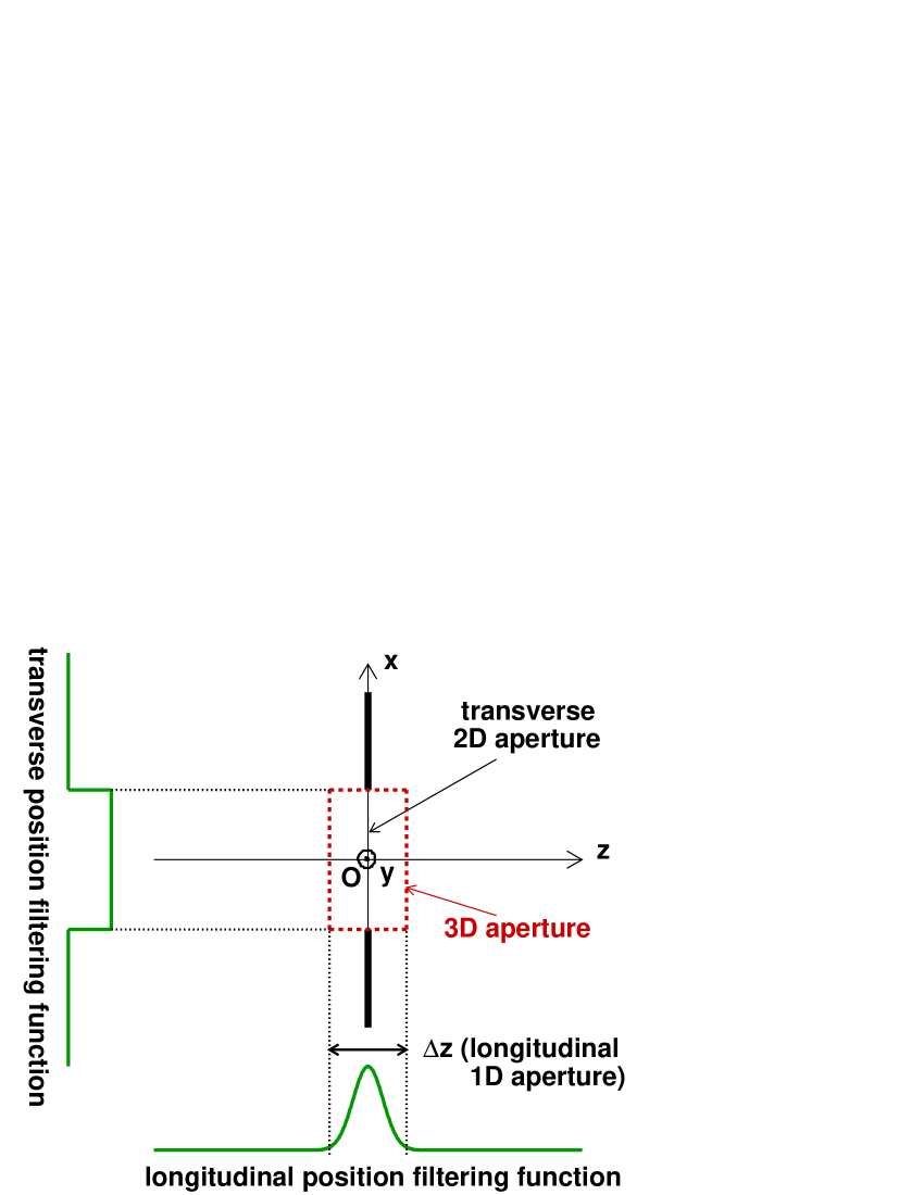
Figure 2: Example of 3D aperture (section in the $(Ox,Oz)$ plane) with the corresponding transverse and longitudinal position filtering functions.

In the case of a uniform filtering, the aperture is the region where the filtering function is non-zero. In the case of a non-uniform filtering, the filtering function can be non-zero everywhere (for example if it is a Gaussian). We are then led to define more generally the aperture as the region outside of which the integral of the filtering function is negligible.

In ( 55), $\Delta z$ does not depend on $x$ and $y$, which is an implicit assumption in the definition ( 46). More generally, the position filtering operator is defined by:

$$\hat{\mathrm{F}}^{\mathcal{A}}=\int\!\mathrm{d}^{3}r\,\sqrt{\widetilde{\delta}^{\mathcal{A}}(\mathbf{r})}\;\left|\,\mathbf{r}\;\right>\,\!\!\,\left<\,\mathbf{r}\,\right|,\hskip 21.33955pt$$ (56)

where $\mathcal{A}$ is the 3D aperture whose shape can be assumed to be more or less complicated and $\widetilde{\delta}^{\mathcal{A}}(\mathbf{r})$ is the position filtering function whose expression can be assumed to be different from a product of the form (​​ 55).

II.3.3 The need to consider kinematics.

From (​​ 56), $\left|\,\left<\,\mathbf{r}\,\left|\left.\hat{\mathrm{F}}^{\mathcal{A}}\,\right|\,\mathbf{k}_{0}\right.\right>\,\right|^{2}$ is proportional to $\widetilde{\delta}^{\mathcal{A}}(\mathbf{r})$. So the state $\hat{\mathrm{F}}^{\mathcal{A}}\left|\,\mathbf{k}_{0}\;\right>\,$ is associated with the momentum PDF of the particle just after its localization at the aperture, when it is about to move away from the diaphragm. Moreover, from (​​ 36), the state $\hat{\mathrm{D}}^{(0)}\left|\,\mathbf{k}_{0}\;\right>\,$ corresponds to the momentum PDF $f_{\mathbf{K}}(\mathbf{k})$ of the particle detected beyond the diaphragm. Since the particle is free after its passage through the aperture, its momentum is conserved until its detection, which suggests that $\hat{\mathrm{D}}^{(0)}$ is nothing other than $\hat{\mathrm{F}}^{\mathcal{A}}$. However, this cannot be the case for the following reason. From (​​ 56), the momentum wave function of the state $\hat{\mathrm{F}}^{\mathcal{A}}\left|\,\mathbf{k}_{0}\;\right>\,$ is expressed by:

$$\,\left<\,\mathbf{k}\,\left|\left.\hat{\mathrm{F}}^{\mathcal{A}}\,\right|\,\mathbf{k}_{0}\right.\right>\,\!=(2\pi)^{-3/2}\;\mathcal{F}^{\mathcal{A}}(\mathbf{k}-\mathbf{k}_{0}),\hskip 21.33955pt$$ (57)

where $\mathcal{F}^{\mathcal{A}}(\mathbf{k}-\mathbf{k}_{0})$ is the Fourier transform of the square root of the position filtering function:

$$\begin{array}[]{l}\displaystyle\mathcal{F}^{\mathcal{A}}(\mathbf{k}-\mathbf{k}_{0})\,\equiv\,(2\pi)^{-3/2}\vspace{0.1cm}\\ \displaystyle\hskip 49.79231pt\times\!\!\int\!\mathrm{d}^{3}r\;\sqrt{\widetilde{\delta}^{\mathcal{A}}(\mathbf{r})}\;\exp\left[\,-\mathrm{i}(\mathbf{k}-\mathbf{k}_{0})\,\boldsymbol{.}\,\mathbf{r}\,\right].\end{array}\hskip 21.33955pt$$ (60)

If $\hat{\mathrm{D}}^{(0)}$ is equal to $\hat{\mathrm{F}}^{\mathcal{A}}$, the PDF $f_{\mathbf{K}}(\mathbf{k})$ is obtained by substituting (​​ 57) into (​​ 36). Then, the widths $\Delta{k_{x}}$, $\Delta{k_{y}}$ and $\Delta{k_{z}}$ of this PDF are those of the distribution associated with the Fourier transform $\mathcal{F}^{\mathcal{A}}(\mathbf{k}-\mathbf{k}_{0})$ and are therefore related to the widths $\Delta x$, $\Delta y$ and $\Delta z$ of the 3D aperture by the uncertainty relations. However, if $\Delta x$ for example is small enough, the relation $\Delta x\Delta{k_{x}}\gtrsim 1$ implies that $\Delta{k_{x}}$ can be sufficiently large so that $|{k_{x}}|>k_{0}$ with non-zero probability and therefore the relation (​​ 2) is not satisfied in such a case. However, this is not possible because (​​ 2) results from kinematics and is moreover confirmed by experiment. This issue comes from the fact that the position wave function of the state $\hat{\mathrm{F}}^{\mathcal{A}}\left|\,\mathbf{k}_{0}\;\right>\,$ is localized in the 3D aperture $\mathcal{A}$ and that consequently its momentum wave function is spread out, which results in a spreading of the distribution of the momentum modulus and therefore of the energy. For (​​ 2) to be satisfied, we are led to assume that $\hat{\mathrm{D}}^{(0)}$ is not simply equal to $\hat{\mathrm{F}}^{\mathcal{A}}$ but is rather of the form:

$$\hat{\mathrm{D}}^{(0)}=\,\hat{\mathrm{F}}^{k_{0}}\;\hat{\mathrm{F}}^{\mathcal{A}},$$ (61)

where $\hat{\mathrm{F}}^{k_{0}}$ is an energy-momentum filtering operator whose role is to act on the state $\hat{\mathrm{F}}^{\mathcal{A}}\left|\,\mathbf{k}_{0}\;\right>\,$, which is then a localized transitional state, to obtain a final state of same energy as that of the initial state.

II.3.4 Energy-momentum filtering operator.

The filtering operator $\hat{\mathrm{F}}^{k_{0}}$ must be associated with the domain $\mathcal{K}_{0}$ of the momentum space that corresponds to the vectors $\mathbf{k}$ compatible with kinematics. So we define, using an expression similar to (​​ 56):

$$\hat{\mathrm{F}}^{k_{0}}\equiv\!\int\mathrm{d}^{3}k\;\sqrt{\widetilde{\delta}^{\,\mathcal{K}_{0}}(\mathbf{k})}\;\left|\,\mathbf{k}\;\right>\,\!\!\,\left<\,\mathbf{k}\,\right|,$$ (62)

where $\widetilde{\delta}^{\,\mathcal{K}_{0}}(\mathbf{k})$ is a momentum-energy filtering function which must represent the weight with which the filtering operator selects the result $\mathbf{k}$ from the value at $\mathbf{k}$ of the momentum wave function in the localized transitional state $\hat{\mathrm{F}}^{\mathcal{A}}\left|\,\mathbf{k}_{0}\;\right>\,$. From (​​ 2) and (​​ 3), we are led to assume that this function is of the form:

$$\widetilde{\delta}^{\,\mathcal{K}_{0}}(\mathbf{k})\equiv C\;\widetilde{\delta}^{\,\Delta k}\!\left(|\mathbf{k}|-k_{0}\right)\;\delta_{1\,\mathrm{sgn}[{k_{z}}]},\hskip 14.22636pt$$ (63)

where $C$ is a normalization constant that will be calculated below, $\widetilde{\delta}^{\,\Delta k}\left(|\mathbf{k}|-k_{0}\right)$ is a function of the modulus of $\mathbf{k}$ forming a peak centered at $|\mathbf{k}|=k_{0}$ and of width $\Delta k$ close to zero (in accordance with (​​ 2)) and the Kronecker delta $\delta_{1\,\mathrm{sgn}[{k_{z}}]}$ ensures that $\widetilde{\delta}^{\,\mathcal{K}_{0}}(\mathbf{k})$ is zero if ${k_{z}}\leq 0$ (in accordance with (​​ 3)). From (​​ 63), using the spherical coordinates, the normalization to 1 of $\widetilde{\delta}^{\,\mathcal{K}_{0}}(\mathbf{k})$ is expressed by:

$$\!\!1=C\!\!\int_{0}^{\infty}\!\!\!\!\!\!\mathrm{d}k\;k^{2}\,\widetilde{\delta}^{\,\Delta k}\!\left(k\!-\!k_{0}\right)\!\!\int_{0}^{\pi}\!\!\!\!\!\mathrm{d}\theta\,\sin\!\theta\,\delta_{1\,\mathrm{sgn}[\cos\theta]}\!\int_{0}^{2\pi}\!\!\!\!\!\!\mathrm{d}\phi.\hskip 21.33955pt$$ (64)

Since $\Delta k$ is close to zero, we can replace $\widetilde{\delta}^{\,\Delta k}\left(k-k_{0}\right)$ by $\delta(k-k_{0})$ in the integral over $k$ whose value is therefore close to ${k_{0}}^{2}$. Then, (​​ 64) implies: $C\simeq{k_{0}}^{\!-2}\,(2\pi)^{-1}$. Substituting (​​ 63) with this value of $C$ into (​​ 62), we get:

$$\begin{array}[]{l}\displaystyle\hat{\mathrm{F}}^{k_{0}}\simeq\,(2\pi)^{-1/2}\,k_{0}^{-1}\vspace{0.2cm}\\ \displaystyle\hskip 28.45274pt\times\!\!\int\!\mathrm{d}^{3}k\;\sqrt{\widetilde{\delta}^{\,\Delta k}\!\left(|\mathbf{k}|-k_{0}\right)}\;\delta_{1\,\mathrm{sgn}[{k_{z}}]}\;\left|\,\mathbf{k}\;\right>\,\!\!\,\left<\,\mathbf{k}\,\right|.\end{array}\hskip 21.33955pt$$ (67)

We can interpret $\hat{\mathrm{F}}^{k_{0}}$ as an operator which represents an energy-momentum measurement including a measurement of the momentum modulus (in other words of the energy) giving the result $\hbar k_{0}$ with near certainty and a measurement of the momentum longitudinal component giving the result $\hbar{k_{z}}>0$.

II.3.5 Matrix element of the momentum part of the diffraction operator.

Substituting (​​ 56) - in which we insert the identity operator $\int\mathrm{d}^{3}k\,\left|\,\mathbf{k}\;\right>\,\!\,\left<\,\mathbf{k}\,\right|$ after $\left|\,\mathbf{r}\;\right>\,\!\,\left<\,\mathbf{r}\,\right|$, and (​​ 67) into (​​ 61), and given (​​ 60), we obtain:

$$\!\!\!\!\begin{array}[]{l}\displaystyle\hat{\mathrm{D}}^{(0)}\!\simeq\,(2\pi)^{-2}\,k_{0}^{-1}\!\!\int\!\mathrm{d}^{3}k\,\sqrt{\widetilde{\delta}^{\,\Delta k}\!\left(|\mathbf{k}|\!-\!k_{0}\right)}\;\delta_{1\,\mathrm{sgn}[{k_{z}}]}\vspace{0.1cm}\\ \displaystyle\hskip 78.24507pt\times\!\!\int\!\mathrm{d}^{3}k^{\prime}\;\mathcal{F}^{\mathcal{A}}(\mathbf{k}-\mathbf{k}^{\prime})\;\left|\,\mathbf{k}\;\right>\,\!\!\,\left<\,\mathbf{k}^{\prime}\,\right|.\end{array}\hskip 18.49411pt$$ (70)

Hence, instead of (​​ 57):

$$\begin{array}[]{l}\displaystyle\,\left<\,\mathbf{k}\,\left|\left.\hat{\mathrm{D}}^{(0)}\,\right|\,\mathbf{k}_{0}\right.\right>\,\simeq(2\pi)^{-2}\,k_{0}^{-1}\vspace{0.2cm}\\ \displaystyle\hskip 42.67912pt\times\sqrt{\widetilde{\delta}^{\,\Delta k}\!\left(|\mathbf{k}|-k_{0}\right)}\;\delta_{1\,\mathrm{sgn}[{k_{z}}]}\;\mathcal{F}^{\mathcal{A}}(\mathbf{k}-\mathbf{k}_{0}).\end{array}\hskip 21.33955pt$$ (73)

II.3.6 Photons.

A position filtering operator of the form ( 56), where the projector $\left|\,\mathbf{r}\;\right>\,\!\!\,\left<\,\mathbf{r}\,\right|$ is involved, cannot be used for the photon because the localized photon states are eigenstates of a photon position operator different from the position observable of the non-relativistic case. Several problems were encountered and then finally resolved to construct this photon position operator and, more generally, to elaborate a true quantum mechanics of the photon [21, 22, 23, 24, 25, 26, 27, 28, 29, 30]. The localized photon states are biorthogonal [27] with a specific scalar product [28] and it follows that the appropriate operator to replace the projector $\left|\,\mathbf{r}\;\right>\,\!\!\,\left<\,\mathbf{r}\,\right|$ in the photon case is $\hat{\mathbf{A}}^{(-)}(\mathbf{r},t)\left|\,\!\textup{vac}\!\;\right>\,\!\boldsymbol{.}\!\,\left<\,\!\textup{vac}\!\,\right|\hat{\mathbf{E}}^{(+)}(\mathbf{r},t)$, where $\hat{\mathbf{A}}^{(\pm)}(\mathbf{r},t)$ and $\hat{\mathbf{E}}^{(\pm)}(\mathbf{r},t)$ are the positive and negative frequency field operators of the transverse vector potential and electric field. These field operators are given by [31]:

$$\begin{array}[]{l}\displaystyle\hat{\mathbf{A}}^{(-)}(\mathbf{r},t)=\left[\hat{\mathbf{A}}^{(+)}(\mathbf{r},t)\right]^{\dagger}=\sqrt{\frac{\hbar}{2\varepsilon_{0}}}\;(2\pi)^{-3/2}\vspace{0.1cm}\\ \displaystyle\hskip 14.22636pt\times\!\!\int\!\frac{\mathrm{d}^{3}k}{\sqrt{{\omega}}}\sum_{l=x,y}\!\!\exp\left[\,\mathrm{i}\left({\omega}t-\mathbf{k}\boldsymbol{.}\mathbf{r}\right)\,\right]\mathbf{e}^{(l)}_{\mathbf{k}}\;\hat{a}^{\dagger}(\mathbf{k},l[\mathbf{k}]),\vspace{0.25cm}\\ \displaystyle\hskip 2.84544pt\hat{\mathbf{E}}^{(-)}(\mathbf{r},t)=\left[\hat{\mathbf{E}}^{(+)}(\mathbf{r},t)\right]^{\dagger}=-\frac{\partial}{\partial t}\hat{\mathbf{A}}^{(-)}(\mathbf{r},t),\end{array}\hskip 21.33955pt$$ (77)

where ${\omega}=ck$, $\mathbf{e}^{(l)}_{\mathbf{k}}$ is the unitary vector of the $l[\mathbf{k}]$ axis of a coordinate system such that $z[\mathbf{k}]\parallel\mathbf{k}$ and $\hat{a}^{\dagger}(\mathbf{k},l[\mathbf{k}])$ is the creation operator of a photon of momentum $\hbar\mathbf{k}$ and linearly polarized in the direction of the $l[\mathbf{k}]$ axis. Similarly to (​​ 12), we have:

$$\hat{a}^{\dagger}(\mathbf{k},l[\mathbf{k}])\left|\,\!\textup{vac}\!\;\right>\,\;=\;\left|\,\mathbf{k}\;\right>\,\!\!\,\otimes\,\!\left|\,l\;\right>\,_{\!\!\mathbf{k}},\hskip 21.33955pt$$ (78)

where $\left|\,l\;\right>\,_{\!\!\mathbf{k}}$ is the basis state of linear polarization in the direction of the $l[\mathbf{k}]$ axis. From (​​ 77) and (​​ 78):

$$\!\!\begin{array}[]{l}\displaystyle\hat{\mathbf{A}}^{(-)}(\mathbf{r},t)\left|\,\!\textup{vac}\!\;\right>\,\!\boldsymbol{.}\!\,\left<\,\!\textup{vac}\!\,\right|\hat{\mathbf{E}}^{(+)}(\mathbf{r},t)\,=\,\frac{\mathrm{i}\hbar}{2\varepsilon_{0}}\,(2\pi)^{-3}\vspace{0.15cm}\\ \displaystyle\hskip 8.5359pt\times\!\!\int\!\!\mathrm{d}^{3}k\!\!\int\!\!\mathrm{d}^{3}k^{\prime}\sqrt{k^{\prime}\!/k\,}\,\exp\{\mathrm{i}\,[({\omega}\!-\!{\omega}^{\prime})t\!-\!(\mathbf{k}\!-\!\mathbf{k}^{\prime})\boldsymbol{.}\mathbf{r}]\}\vspace{0.15cm}\\ \displaystyle\hskip 8.5359pt\times\left|\,\mathbf{k}\;\right>\,\!\!\,\left<\,\mathbf{k}^{\prime}\,\right|\,\otimes\,\!\!\sum_{l=x,y}\sum_{l^{\prime}=x,y}{\mathbf{e}^{(l)}_{\mathbf{k}}}\!\boldsymbol{.}\,\mathbf{e}^{(l^{\prime})}_{\mathbf{k}^{\prime}}\left|\,l\;\right>\,_{\!\!\mathbf{k}}\;\,{}_{\mathbf{k}^{\prime}\!\!\!}\,\left<\,l^{\prime}\,\right|.\end{array}\hskip 21.33955pt$$ (82)

The photon has a spin 1 and this implies that its spin projection eigenstates are equivalent to vectors of complex components in the basis $\{\mathbf{e}^{(x)}_{\mathbf{k}},\mathbf{e}^{(y)}_{\mathbf{k}},\mathbf{e}^{(z)}_{\mathbf{k}}\}$ [32]. Moreover, the basis states $\left|\,l\;\right>\,_{\!\!\mathbf{k}}$ are specific linear combinations of the spin projection eigenstates [31, 33] such that $\left|\,l\;\right>\,_{\!\!\mathbf{k}}$ is equivalent to the real vector ${\mathbf{e}^{(l)}_{\mathbf{k}}}$. Therefore: ${\mathbf{e}^{(l)}_{\mathbf{k}}}\boldsymbol{.}\,\mathbf{e}^{(l^{\prime})}_{\mathbf{k}^{\prime}}=\,{\mathbf{e}^{(l)}_{\mathbf{k}}}^{*}\!\boldsymbol{.}\,\mathbf{e}^{(l^{\prime})}_{\mathbf{k}^{\prime}}=\,_{\mathbf{k}\!\!\!}\,\left<\,l\left|\,l^{\prime}\right.\right>\,_{\!\!\mathbf{k}^{\prime}}$. So the double sum over $l$ and $l^{\prime}$ in ( 82) is the product of the identity operator by itself, successively expressed by the closure relations of the bases $\{\left|\,x\;\right>\,_{\!\!\mathbf{k}},\left|\,y\;\right>\,_{\!\!\mathbf{k}}\}$ and $\{\left|\,x\;\right>\,_{\!\!\mathbf{k}^{\prime}},\left|\,y\;\right>\,_{\!\!\mathbf{k}^{\prime}}\}$. The action of the operator $\hat{\mathbf{A}}^{(-)}(\mathbf{r},t)\left|\,\!\textup{vac}\!\;\right>\,\!\boldsymbol{.}\!\,\left<\,\!\textup{vac}\!\,\right|\hat{\mathbf{E}}^{(+)}(\mathbf{r},t)$ therefore has no effect on the polarization states so we can just consider its restriction to the subspace of the momentum states. So, replacing in (​​ 56) $\left|\,\mathbf{r}\;\right>\,\!\,\left<\,\mathbf{r}\,\right|$ by the right-hand side of ( 82) without the double sum over $l$ and $l^{\prime}$ and multiplying by the factor $-2\mathrm{i}\varepsilon_{0}/\hbar$ to obtain the same dimension as that of $\hat{\mathrm{F}}^{\mathcal{A}}$ (length to the power $-3/2$), we are led to assume that the position filtering operator for the photon is:

$$\begin{array}[]{l}\displaystyle\hat{\mathrm{F}}^{\mathcal{A}}_{\textup{phot}}(t)=(2\pi)^{-3}\!\!\int\!\mathrm{d}^{3}r\;\sqrt{\widetilde{\delta}^{\mathcal{A}}(\mathbf{r})}\;\!\int\!\!\mathrm{d}^{3}k\!\!\int\!\!\mathrm{d}^{3}k^{\prime}\vspace{0.1cm}\\ \displaystyle\hskip 7.11317pt\times\,\sqrt{k^{\prime}\!/k\,}\,\exp\{\mathrm{i}\,[({\omega}\!-\!{\omega}^{\prime})t\!-\!(\mathbf{k}\!-\!\mathbf{k}^{\prime})\boldsymbol{.}\mathbf{r}]\}\left|\,\mathbf{k}\;\right>\,\!\!\,\left<\,\mathbf{k}^{\prime}\,\right|.\end{array}\hskip 21.33955pt$$ (85)

Furthermore, we express the momentum part of the diffraction operator in a form similar to ( 61):

$$\hat{\mathrm{D}}^{(0)}_{\textup{phot}}(t)=\hat{\mathrm{F}}^{k_{0}}\;\hat{\mathrm{F}}^{\mathcal{A}}_{\textup{phot}}(t).\hskip 21.33955pt$$ (86)

Then, substituting ( 67) and ( 85) into ( 86) - and given ( 60) - we finally obtain:

$$\begin{array}[]{l}\displaystyle\hat{\mathrm{D}}^{(0)}_{\textup{phot}}(t)\simeq(2\pi)^{-2}k_{0}^{-1}\!\!\!\int\!\!\mathrm{d}^{3}k\,\sqrt{\widetilde{\delta}^{\,\Delta k}\!\left(|\mathbf{k}|\!-\!k_{0}\right)}\;\delta_{1\,\mathrm{sgn}[{k_{z}}]}\vspace{0.15cm}\\ \displaystyle\hskip 2.84544pt\times\!\!\int\!\!\mathrm{d}^{3}k^{\prime}\sqrt{k^{\prime}\!/k\,}\,\exp[\,\mathrm{i}({\omega}\!-\!{\omega}^{\prime})t\,]\;\mathcal{F}^{\mathcal{A}}(\mathbf{k}\!-\!\mathbf{k}^{\prime})\left|\,\mathbf{k}\;\right>\,\!\!\,\left<\,\mathbf{k}^{\prime}\,\right|\!.\end{array}\hskip 21.33955pt$$ (89)

By calculating the matrix element $\,\left<\,\mathbf{k}\,\left|\left.\hat{\mathrm{D}}^{(0)}_{\textup{phot}}(t)\,\right|\,\mathbf{k}_{0}\right.\right>\,$ from ( 89), we get an expression with the factor $\exp[\mathrm{i}({\omega}-{\omega}_{0})t]$. Now, from ( 2), $k\!\simeq\!k_{0}$, and so ${\omega}\!\simeq\!{\omega}_{0}$. Therefore, the matrix element in question does not actually depend on time and we find that its expression is nothing other than ( 73). This relation can therefore be used both for non-relativistic particles and for photons.

II.3.7 Characteristics of the measurement process.

From (​​ 61) and (​​ 86), we see that the momentum part $\hat{\mathrm{D}}^{(0)}$ of the diffraction operator depends on the momentum modulus $k_{0}$ of the incident particle. Therefore, the initial state is changed by the action of an operator which depends on this initial state itself. This reflects the fact that the diaphragm and the particle form an inseparable system during the measurement, in accordance with the Copenhagen interpretation of quantum mechanics.

Moreover, using (​​ 56), (​​ 67) and (​​ 85), we can verify that the product of operators on the right-hand sides of (​​ 61) and (​​ 86) is not commutative. This non-commutativity imposes the order in which the operators act to create the final state from the initial state. This order is related to the temporal unfolding of an irreversible process whose sequence is as follows: initial state $\rightarrow$ position measurement ($\hat{\mathrm{F}}^{\mathcal{A}}$) $\rightarrow$ localized transitional state $\rightarrow$ energy-momentum measurement ($\hat{\mathrm{F}}^{k_{0}}$) $\rightarrow$ final state $\rightarrow$ measurement of momentum and polarization (detectors). The two first measurements ($\hat{\mathrm{D}}^{(0)}$) are not equivalent to one measurement to which the uncertainty relations apply. These relations are satisfied for each of the two measurements. Let $\Delta x$, $\Delta{k_{x}}$ be the uncertainties of the first measurement which creates the localized transitional state and $\Delta^{\prime}x$, $\Delta^{\prime}{k_{x}}$ those of the second measurement which creates the final state. So $\Delta x$ is the width of the aperture and $\Delta^{\prime}{k_{x}}$ is the width of the distribution of ${k_{x}}$ in the final state. In this state, we have: $-k\leq{k_{x}}\leq+k$, so $\Delta^{\prime}{k_{x}}\lesssim 2k$. Hence, because of kinematics [Eq. (​​ 2)]: $\Delta^{\prime}{k_{x}}\lesssim 2k_{0}$ which is finite. Therefore, if $\Delta x$ is small enough, we then have: $\Delta x\Delta^{\prime}{k_{x}}\lesssim 1$ but this is not a problem because $\Delta x$ is associated with the first measurement while $\Delta^{\prime}{k_{x}}$ is associated with the second measurement. On the other hand, we have: $\Delta x\Delta{k_{x}}\gtrsim 1$ and $\Delta^{\prime}x\Delta^{\prime}{k_{x}}\gtrsim 1$, where $\Delta^{\prime}x$ corresponds to the extent of the diffracted wave. We also have the relations: $\Delta t\Delta{\omega}\gtrsim 1$ and $\Delta^{\prime}t\Delta^{\prime}{\omega}\gtrsim 1$ between the lifetimes and the widths in energy of the transitional state and of the final state. We can assume that $\Delta t\simeq\Delta z/v$ where $v$ is the speed of the particle. Because of the Huygens-Fresnel principle, it is expected that $\Delta z\simeq 0$ (Sec.  II.3.2). So $\Delta t\simeq 0$. Moreover, given (​​ 2), we have $\Delta^{\prime}{\omega}\simeq 0$. Hence: $\Delta t\Delta^{\prime}{\omega}\lesssim 1$.

II.4 Polarization amplitudes of the detected particles

II.4.1 Non-relativistic particles.

The quantization axis $Z[\mathbf{k}]$ belongs to a coordinate system $\{X[\mathbf{k}],Y[\mathbf{k}],Z[\mathbf{k}]\}$ defined by $L[\mathbf{k}]=\mathcal{R}(\Phi,\Theta,\Psi)\,l[\mathbf{k}]$ ($L=X,Y,Z$; $l=x,y,z$), where $\mathcal{R}(\Phi,\Theta,\Psi)$ is a rotation whose Euler angles can be chosen arbitrarily and $\{x[\mathbf{k}],y[\mathbf{k}],z[\mathbf{k}]\}$ is the coordinate system attached to the particle. Moreover, according to (​​ 4): $l[\mathbf{k}]=\mathcal{R}(\phi,\theta,0)\,l[\mathbf{k}_{0}]$. The rotation of the eigenstates has the same Euler angle as the rotation of the axes because a physical system in a given eigenstate must rotate with the coordinate system associated with the quantization axis to remain in this eigenstate. Therefore:

$$\begin{array}[]{ccl}\left|\,\sigma\;\right>\,_{\!\!Z[\mathbf{k}],\Psi}&=&\hat{\mathrm{R}}^{({s})}(\Phi,\Theta,\Psi)\left|\,\sigma\;\right>\,_{\!\!z[\mathbf{k}]},\vspace{0.15cm}\\ \left|\,\sigma\;\right>\,_{\!\!z[\mathbf{k}]}&=&\hat{\mathrm{R}}^{({s})}(\,\phi,\theta,0\,)\left|\,\sigma\;\right>\,_{\!\!z[\mathbf{k}_{0}]}\,.\end{array}\hskip 21.33955pt$$ (92)

In the present case, where the directions of the $L[\mathbf{k}]$ axes are defined by the rotation $\mathcal{R}(\Phi,\Theta,\Psi)$, the angle $\Psi$ must be mentioned in the notation $\left|\,\sigma\;\right>\,_{\!\!Z[\mathbf{k}],\Psi}$ because $Z[\mathbf{k}]$ only depends on $\Phi,\Theta$ whereas the rotation operator $\hat{\mathrm{R}}^{({s})}(\Phi,\Theta,\Psi)$ (so a priori the resulting state) also depends on $\Psi$.

To express the final polarization amplitudes (quantization axis $Z[\mathbf{k}]$) as a function of the initial amplitudes (quantization axis $Z[\mathbf{k}_{0}]$), we multiply the relation (​​ 17) on the left by ${}_{\;Z[\mathbf{k}],\Psi}\!\!\,\left<\,\sigma\,\right|$ and we insert the identity operator $\sum_{\sigma^{\prime}}\!\left|\,\!\sigma^{\prime}\!\;\right>\,\!_{\!\!Z[\mathbf{k}_{0}],\Psi_{0}}\;{}_{Z[\mathbf{k}_{0}],\Psi_{0}\!\!\!}\,\left<\,\!\sigma^{\prime}\!\,\right|$ before the ket $\left|\,\chi^{({s})}_{\textup{in}}\;\right>\,$. We then use (​​ 92) and the relation: $\hat{\mathrm{R}}^{({s})}(\alpha,\beta,\gamma)^{\dagger}=\hat{\mathrm{R}}^{({s})}(\alpha,\beta,\gamma)^{-1}=\hat{\mathrm{R}}^{({s})}(-\gamma,-\beta,-\alpha)$ which results from the unitarity of the rotation operators. We get

$$\begin{array}[]{l}_{\;Z[\mathbf{k}],\Psi}\!\!\,\left<\,\!\sigma\left|\,\chi^{({s})}_{\textup{out}}(\mathbf{k})\!\right.\right>\,\!=\sum_{\sigma^{\prime}}\vspace{0.1cm}\\ _{\;\;\;\,z[\mathbf{k}_{0}]}\!\!\,\left<\,\!\sigma\!\,\left|\left.\hat{\mathrm{R}}^{({s})}(0,-\theta,-\phi)\,\hat{\mathrm{R}}^{({s})}(-\Psi,-\Theta,-\Phi)\right.\right.\right.\vspace{0.15cm}\\ \displaystyle\hskip 35.56593pt\times\left.\left.\left.\!\!\hat{\mathrm{R}}^{({s})}(\alpha_{1},\alpha_{2},\alpha_{3})\,\hat{\mathrm{R}}^{({s})}(\Phi_{0},\Theta_{0},\Psi_{0})\,\right|\,\!\sigma^{\prime}\!\right.\right>\,_{\!\!z[\mathbf{k}_{0}]}\vspace{0.15cm}\\ \displaystyle\hskip 106.69783pt\times\,_{Z[\mathbf{k}_{0}],\Psi_{0}\!\!\!}\,\left<\,\!\sigma^{\prime}\!\left|\,\!\chi^{({s})}_{\textup{in}}\!\right.\right>\,\!,\end{array}\hskip 14.22636pt$$ (97)

where $Z[\mathbf{k}]=Z[\mathbf{k};\Phi,\Theta]$, $Z[\mathbf{k}_{0}]=Z[\mathbf{k}_{0};\Phi_{0},\Theta_{0}]$, $\alpha_{j}\equiv\alpha_{j}(\mathbf{k})$ and $\mathbf{k}\equiv\mathbf{k}(k,\theta,\phi)$. The matrix element of the product of the four rotation operators can be calculated from the standard formula

$$\,\left<\,\!\sigma\!\,\left|\left.\hat{\mathrm{R}}^{({s})}(\alpha,\beta,\gamma)\,\right|\,\!\sigma^{\prime}\right.\right>\,\!=\exp[-\mathrm{i}(\sigma\alpha\!+\!\sigma^{\prime}\gamma)]\;d_{\sigma\sigma^{\prime}}^{\,({s})}(\beta)\,,\hskip 21.33955pt$$ (98)

where $(d_{\sigma\sigma^{\prime}}^{\,({s})}(\beta))$ is a $(2{s}+1)\!\times\!(2{s}+1)$ matrix whose expression is known [33].

II.4.2 Relativistic particles.

The quantization axis $Z[\mathbf{k}]$ must have the same direction as that of the momentum $\mathbf{k}$. Since $z[\mathbf{k}]\parallel\mathbf{k}$ (Eq. (​​ 4)], this implies $Z[\mathbf{k}]=z[\mathbf{k}]$. We then have $\Theta=0$ and $\mathcal{R}(\Phi,0,\Psi)=\mathcal{R}(\Phi+\Psi,0,0)=\mathcal{R}(0,0,\Phi+\Psi)$ which is a rotation of arbitrary angle $\Phi+\Psi$ around $z[\mathbf{k}]$. To simplify, we choose $\Phi=0$ and $\mathcal{R}(0,0,\Psi)$. We then apply the first relation of (​​ 92) to the rotation $\hat{\mathrm{R}}^{({s})}(0,0,\Psi)$. Using (​​ 98) and the property $d_{\sigma\sigma^{\prime}}^{\,({s})}(0)=\delta_{\sigma\sigma^{\prime}}$ [33], this leads to: $\left|\,\sigma\;\right>\,_{\!\!Z[\mathbf{k}],\Psi}=\exp(-\mathrm{i}\sigma\Psi)\left|\,\sigma\;\right>\,_{\!\!z[\mathbf{k}]}$. Then, since $Z[\mathbf{k}]=z[\mathbf{k}]$ and $z[\mathbf{k}]\parallel\mathbf{k}$, we will use the notation $\left|\,\sigma\;\right>\,_{\!\!\mathbf{k},\Psi}$ for simplicity. Finally,

$$\left|\,\sigma\;\right>\,_{\!\!\mathbf{k},\Psi}\equiv\hat{\mathrm{R}}^{({s})}(0,0,\Psi)\left|\,\sigma\;\right>\,_{\!\!\mathbf{k}}=\exp\,(-\mathrm{i}\sigma\Psi)\left|\,\sigma\;\right>\,_{\!\!\mathbf{k}}.\hskip 21.33955pt$$ (99)

Substituting into (​​ 97), we get:

$$\begin{array}[]{l}\,_{\mathbf{k}\!\!\!}\,\left<\,\!\sigma\left|\,\chi^{({s})}_{\textup{out}}(\mathbf{k})\!\right.\right>\,=\sum_{\sigma^{\prime}}\vspace{0.1cm}\\ \displaystyle\hskip 7.11317pt\times\,\,_{\mathbf{k}_{0}\!\!\!}\,\left<\,\!\sigma\!\,\left|\left.\hat{\mathrm{R}}^{({s})}(0,-\theta,-\phi)\,\hat{\mathrm{R}}^{({s})}(\alpha_{1},\alpha_{2},\alpha_{3})\,\right|\,\!\sigma^{\prime}\!\right.\right>\,_{\!\!\mathbf{k}_{0}}\vspace{0.1cm}\\ \displaystyle\hskip 85.35826pt\times\,_{\mathbf{k}_{0}\!\!\!}\,\left<\,\!\sigma^{\prime}\!\left|\,\!\chi^{({s})}_{\textup{in}}\!\right.\right>\,\!.\end{array}\hskip 21.33955pt$$ (103)

In the rest of this subsection, we apply the model to the case of the photon.

II.4.3 Helicity amplitudes of the detected photons.

Since the photon is relativistic and has a spin 1, its spin component eigenstates are the helicity states $\left|\,+1\;\right>\,_{\!\!\mathbf{k}}$, $\left|\,0\;\right>\,_{\!\!\mathbf{k}}$, and $\left|\,-1\;\right>\,_{\!\!\mathbf{k}}$. However, the photon is also massless, so its helicity can only have the values $\pm 1$ [16]; the value zero is impossible, whatever the momentum. Hence:

$$\,{}_{\mathbf{k}\!\!\!}\,\left<\,0\left|\,\chi^{({1})}_{\textup{out}}(\mathbf{k})\right.\right>\,=\,\,_{\mathbf{k}_{0}\!\!\!}\,\left<\,0\left|\,\chi^{({1})}_{\textup{in}}\right.\right>\,\,=\;0.\hskip 21.33955pt$$ (104)

This relation determines the functions $\alpha_{1}[\mathbf{k}(k,\theta,\phi)]$ and $\alpha_{2}[\mathbf{k}(k,\theta,\phi)]$. Indeed, substituting it into (​​ 103) applied to ${s}=1$ and $\sigma=0$, we obtain:

$$\begin{array}[]{l}\displaystyle 0\;=\sum_{\sigma^{\prime}=\pm 1}\,{}_{\mathbf{k}_{0}\!\!\!}\,\left<\,\!0\!\,\left|\left.\hat{\mathrm{R}}^{({1})}(0,-\theta,-\phi)\right.\right.\right.\vspace{0.1cm}\\ \displaystyle\hskip 42.67912pt\left.\left.\left.\times\,\hat{\mathrm{R}}^{({1})}(\alpha_{1},\alpha_{2},\alpha_{3})\,\right|\,\!\sigma^{\prime}\!\right.\right>\,_{\!\!\mathbf{k}_{0}}\,\,{}_{\mathbf{k}_{0}\!\!\!}\,\left<\,\sigma^{\prime}\left|\,\chi^{({1})}_{\textup{in}}\right.\right>\,\!,\end{array}\hskip 21.33955pt$$ (107)

which must be satisfied whatever the initial state. Hence:

$$\,{}_{\mathbf{k}_{0}\!\!\!}\,\left<\,\!0\!\,\left|\left.\hat{\mathrm{R}}^{({1})}(0,-\theta,-\phi)\,\hat{\mathrm{R}}^{({1})}(\alpha_{1},\alpha_{2},\alpha_{3})\,\right|\,\!\pm 1\!\right.\right>\,_{\!\!\mathbf{k}_{0}}\!=0.\;\hskip 21.33955pt$$ (108)

We then express the left-hand side by using (​​ 98) applied to ${s}\!=\!1$ and where the matrix $(d_{\sigma\sigma^{\prime}}^{\,({1})}(\beta))$ is given by [33]:

$$\!\!\left(d_{\sigma\sigma^{\prime}}^{\,({1})}(\beta)\right)\!=\!\frac{1}{2}\!\left(\begin{array}[]{ccc}\displaystyle 1\!+\!\cos\beta&\displaystyle-\sqrt{2}\sin\beta&\displaystyle 1\!-\!\cos\beta\vspace{0.1cm}\\ \displaystyle\sqrt{2}\sin\beta&\displaystyle 2\cos\beta&\displaystyle-\sqrt{2}\sin\beta\vspace{0.1cm}\\ \displaystyle 1\!-\!\cos\beta&\displaystyle\sqrt{2}\sin\beta&\displaystyle 1\!+\!\cos\beta\end{array}\right)\!.\hskip 21.33955pt$$ (112)

(Note that the order of the values of $\sigma$ and $\sigma^{\prime}$ is: $+1,0,-1$). This leads to the equations:

$$\begin{array}[]{c}\sin\theta\sin(\phi-\alpha_{1})=0,\vspace{0.2cm}\\ \sin\theta\cos\alpha_{2}\cos(\phi-\alpha_{1})-\cos\theta\sin\alpha_{2}=0.\end{array}\hskip 21.33955pt$$ (115)

The first equation implies $\alpha_{1}(\mathbf{k})=\phi+n\pi$, $n=0,1$. Substituting into the second equation, we get: $\alpha_{2}(\mathbf{k})=(-1)^{n}\theta+n^{\prime}\pi$, $n^{\prime}=0,1$. If $\phi=\theta=0$, we then have: $\mathbf{k}=\mathbf{k}_{0}$, which implies $\alpha_{1}(\mathbf{k}_{0})=n\pi$ and $\alpha_{2}(\mathbf{k}_{0})=n^{\prime}\pi$. However, if $\mathbf{k}=\mathbf{k}_{0}$, there is no reason for the spin polarization state to change. Hence, from (​​ 17), $\hat{\mathrm{R}}^{({1})}\!\left[\alpha_{1}(\mathbf{k}_{0}),\alpha_{2}(\mathbf{k}_{0}),\alpha_{3}(\mathbf{k}_{0})\right]$ is equal to the identity operator, which implies: $\alpha_{1}(\mathbf{k}_{0})=\alpha_{2}(\mathbf{k}_{0})=\alpha_{3}(\mathbf{k}_{0})=0$. Therefore: $n=n^{\prime}=0$ and we get

$$\alpha_{1}(\mathbf{k})=\phi,\hskip 21.33955pt\alpha_{2}(\mathbf{k})=\theta,\hskip 21.33955pt$$ (116)

$$\;\alpha_{3}(\mathbf{k}_{0})=0.\hskip 21.33955pt$$ (117)

From (​​ 98), (​​ 112) and (​​ 116), the matrix whose elements appear in the right-hand side of (​​ 103) is given by:

$$\begin{array}[]{l}\displaystyle\!\left(\,{}_{\mathbf{k}_{0}\!\!\!}\,\left<\,\sigma\,\left|\left.\hat{\mathrm{R}}^{(1)}(0,-\theta,-\phi)\,\hat{\mathrm{R}}^{(1)}[\phi,\theta,\alpha_{3}(\mathbf{k})]\,\right|\,\sigma^{\prime}\right.\right>\,_{\!\!\mathbf{k}_{0}}\,\right)\vspace{0.2cm}\\ \displaystyle\hskip 42.67912pt\;=\left(\begin{array}[]{ccc}\displaystyle\exp\left[-\mathrm{i}\alpha_{3}(\mathbf{k})\right]&\;0&0\vspace{0.2cm}\\ 0&\;1&0\vspace{0.2cm}\\ 0&\;0&\displaystyle\exp\left[\mathrm{i}\alpha_{3}(\mathbf{k})\right]\end{array}\,\right)\!.\end{array}$$ (123)

Finally, from (​​ 103), (​​ 116) and (​​ 123):

$$\,{}_{\mathbf{k}\!\!\!}\,\left<\,\!\sigma\left|\,\chi^{({1})}_{\textup{out}}(\mathbf{k})\!\right.\right>\,\!=\exp\left[-\mathrm{i}\sigma\alpha_{3}(\mathbf{k})\,\right]\,\,_{\mathbf{k}_{0}\!\!\!}\,\left<\,\!\sigma\left|\,\chi^{({1})}_{\textup{in}}\!\right.\right>\,.\hskip 21.33955pt$$ (124)

Diffraction causes a phase shift of $2\alpha_{3}(\mathbf{k})$ between the amplitudes of the helicity states $\left|\,\pm 1\;\right>\,$ and conserves the modulus of each of these amplitudes.

II.4.4 Linear polarization amplitudes of the detected photons.

It is useful to express the amplitudes of linear polarization for any direction of the maximum transmission axis of the analyzer. We associate with the analyzer the coordinate system $\{X[\mathbf{k}],Y[\mathbf{k}],z[\mathbf{k}]\}$ associated with the quantization axis $z[\mathbf{k}]$ and we assume by convention that the axis $X[\mathbf{k}]=\mathcal{R}(0,0,\Psi)\,x[\mathbf{k}]\equiv x[\mathbf{k},\Psi]$ is the maximum transmission axis whose direction is therefore defined by the choice of the value of $\Psi$.

The helicity states and the basis states of linear polarization in the directions of the $l[\mathbf{k},\Psi]$ axes ($l=x,y$) are related by [33, 31]:

$$\left|\,\xi\;\right>\,_{\!\!\mathbf{k},\Psi}=\displaystyle\frac{-\xi}{\sqrt{2}}\left(\;\left|\,x\;\right>\,_{\!\!\mathbf{k},\Psi}+\mathrm{i}\,\xi\left|\,y\;\right>\,_{\!\!\mathbf{k},\Psi}\;\right),\hskip 21.33955pt$$ (125)

where $\xi=\pm 1$ is the helicity. According to (​​ 99) applied to the helicity states $\left|\,\xi\;\right>\,_{\!\!\mathbf{k},\Psi}$ and $\left|\,\xi\;\right>\,_{\!\!\mathbf{k}}$ expressed from (​​ 125), the basis states $\left|\,l\;\right>\,_{\!\!\mathbf{k}}$ transform like the real unitary vectors $\mathbf{e}^{(l)}_{\mathbf{k}}$ of the $l[\mathbf{k}]$ axes:

$$\begin{array}[]{lll}\left|\,x\;\right>\,_{\!\!\mathbf{k},\Psi}&=&\;\,\cos\Psi\left|\,x\;\right>\,_{\!\!\mathbf{k}}+\sin\Psi\left|\,y\;\right>\,_{\!\!\mathbf{k}},\vspace{0.2cm}\\ \left|\,y\;\right>\,_{\!\!\mathbf{k},\Psi}&=&\!\!-\sin\Psi\left|\,x\;\right>\,_{\!\!\mathbf{k}}+\cos\Psi\left|\,y\;\right>\,_{\!\!\mathbf{k}},\end{array}\hskip 21.33955pt$$ (128)

which implies in particular:

$$\left|\,y\;\right>\,_{\!\!\mathbf{k},\Psi}=\left|\,x\;\right>\,_{\!\!\mathbf{k},\Psi+\frac{\pi}{2}}.\hskip 21.33955pt$$ (129)

Finally, from (​​ 124), (​​ 125) and (​​ 128), we get:

$$\begin{array}[]{l}\,_{\!\!\mathbf{k},\Psi\!\!\!}\,\left<\,x\left|\,\chi^{({1})}_{\textup{out}}(\mathbf{k})\right.\right>\,=\cos\left[\,\alpha_{3}(\mathbf{k})\!-\!\Psi\,\right]\,\,_{\mathbf{k}_{0}\!\!\!}\,\left<\,\!x\left|\,\chi^{({1})}_{\textup{in}}\right.\right>\vspace{0.2cm}\\ \displaystyle\hskip 71.13188pt\,\;\,-\sin\left[\,\alpha_{3}(\mathbf{k})\!-\!\Psi\,\right]\,\,_{\mathbf{k}_{0}\!\!\!}\,\left<\,\!y\left|\,\chi^{({1})}_{\textup{in}}\right.\right>\,,\end{array}\hskip 21.33955pt$$ (132)

from which we deduce $\,\,{}_{\!\!\mathbf{k},\Psi\!\!\!}\,\left<\,y\left|\,\chi^{({1})}_{\textup{out}}(\mathbf{k})\right.\right>\,$ by using (​​ 129).

II.4.5 Case of an initial state elliptically polarized (photons).

By generalizing (​​ 125), we can express any elliptically polarized initial state in the form:

$$\left|\,\widetilde{\chi}^{({1})}_{\textup{in}}\!\;\right>\,\!\!\equiv-\xi_{0}\!\left(\,\cos\eta_{0}\left|\,x\;\right>\,_{\!\!\mathbf{k}_{0},\zeta_{0}}\!+\mathrm{i}\,\xi_{0}\sin\eta_{0}\left|\,y\;\right>\,_{\!\!\mathbf{k}_{0},\zeta_{0}}\,\right)\!,\hskip 21.33955pt$$ (133)

where $\zeta_{0}$, $\eta_{0}$ and $\xi_{0}$ represent the major axis azimuth, the ellipticity angle, and the handedness, respectively .

The final state resulting from the initial state $\left|\,\widetilde{\chi}^{({1})}_{\textup{in}}\;\right>\,$ is also an elliptically polarized state which we denote $\left|\,\widetilde{\chi}^{({1})}_{\textup{out}}(\mathbf{k})\;\right>\,$. Indeed, by applying (​​ 132) to $\left|\,\widetilde{\chi}^{({1})}_{\textup{in}}\;\right>\,$ defined by (​​ 133) and using (​​ 128), we obtain:

$$\begin{array}[]{rcl}\,_{\!\!\mathbf{k},\Psi\!\!\!}\,\left<\,x\left|\,\widetilde{\chi}^{({1})}_{\textup{out}}(\mathbf{k})\right.\right>&\!\!=\!\!&-\xi_{0}\cos\eta_{0}\cos\left[\,\zeta_{0}\!+\!\alpha_{3}(\mathbf{k})\!-\!\Psi\,\right]\vspace{0.1cm}\\ &&\;\;+\;\mathrm{i}\,\sin\eta_{0}\sin\left[\,\zeta_{0}\!+\!\alpha_{3}(\mathbf{k})\!-\!\Psi\,\right].\end{array}\hskip 21.33955pt$$ (136)

Then, by making the identity operator $\sum_{l=x,y}\left|\,l\;\right>\,_{\!\!\mathbf{k}}\,\,{}_{\mathbf{k}\!\!\!}\,\left<\,l\,\right|$ act on the state $\left|\,\widetilde{\chi}^{({1})}_{\textup{out}}(\mathbf{k})\;\right>\,$ and using successively (​​ 136) (applied with $\Psi=0$), (​​ 129) and (​​ 128), we get:

$$\begin{array}[]{l}\displaystyle\left|\,\widetilde{\chi}^{({1})}_{\textup{out}}(\mathbf{k})\;\right>\,=-\xi_{0}\left[\,\cos\eta_{0}\left|\,x\;\right>\,_{\!\!\mathbf{k},\zeta_{0}+\alpha_{3}(\mathbf{k})}\right.\vspace{0.1cm}\\ \left.\displaystyle\hskip 85.35826pt+\,\mathrm{i}\,\xi_{0}\,\sin\eta_{0}\left|\,y\;\right>\,_{\!\!\mathbf{k},\zeta_{0}+\alpha_{3}(\mathbf{k})}\,\right].\end{array}\hskip 21.33955pt$$ (139)

Comparing with (​​ 133), we see that the ellipticity and the handedness are conserved and that the ellipse axes undergo a rotation of angle $\alpha_{3}(\mathbf{k})$. The major axis azimuth in the transverse plane $\{x[\mathbf{k}],y[\mathbf{k}]\}$ is: $\zeta(\mathbf{k})=\zeta_{0}+\alpha_{3}(\mathbf{k})$.

III Some predictions of the model

III.1 Relative intensity (polarization not measured)

III.1.1 Angular distribution of the final momentum.

From (​​ 36) and (​​ 73), the PDF of the final momentum if the polarization is not measured is expressed by:

$$\begin{array}[]{l}\displaystyle f_{\mathbf{K}}(\mathbf{k})\,\simeq\,{N}^{-1}\,(2\pi)^{-4}k_{0}^{-2}\vspace{0.2cm}\\ \displaystyle\hskip 42.67912pt\times\,\widetilde{\delta}^{\,\Delta k}\!\left(|\mathbf{k}|\!-\!k_{0}\right)\delta_{1\,\mathrm{sgn}[{k_{z}}]}\left|\mathcal{F}^{\mathcal{A}}(\mathbf{k}\!-\!\mathbf{k}_{0})\right|^{2}\!\!.\end{array}\hskip 21.33955pt$$ (142)

Since the experimental setup directly measures the direction of $\mathbf{k}$, it is useful to replace the Cartesian components by the modulus and two angles giving the direction. This change of variables must be done by a one-to-one transformation which must moreover be defined in the half-space ${k_{z}}>0$ because of (​​ 3). The spherical coordinates $k,\theta,\phi$ cannot be used because the associated transformation is not one-to-one (if $\theta=0$, $\phi$ is undetermined and the Jacobian is zero). On the other hand, we can use the diffraction angles $\theta_{x}$ and $\theta_{y}$ [19] which are the projections of the polar angle $\theta$ on the planes $(x,z)$ and $(y,z)$ (Fig. ​​ 3).

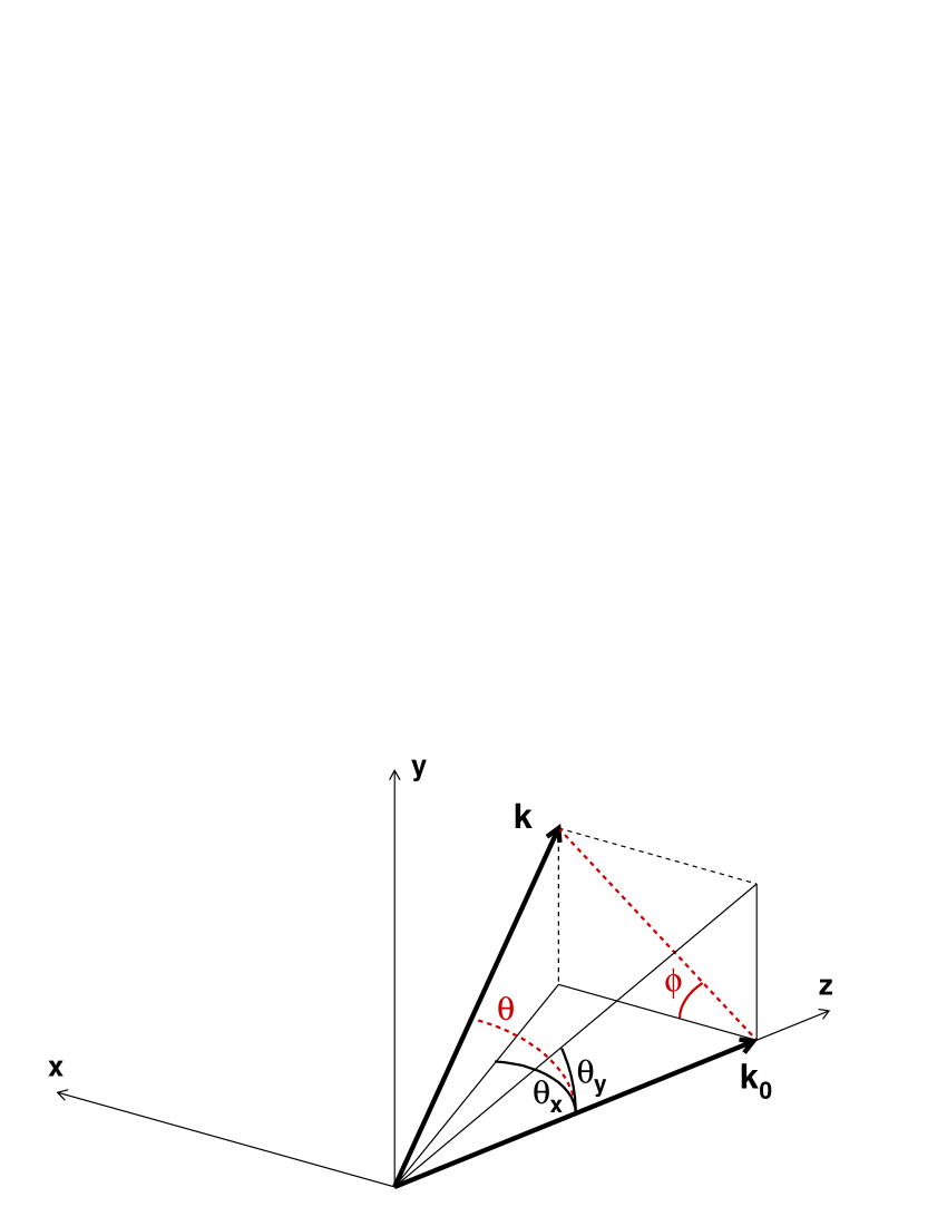
Figure 3: Diffraction angles $\theta_{x}$ and $\theta_{y}$.

The new variables $(k,\theta_{x},\theta_{y})$ are such that: $k>0$, $-\pi/2<\theta_{x}<+\pi/2$, $-\pi/2<\theta_{y}<+\pi/2$ and the required transformation $({k_{x}},{k_{y}},{k_{z}})\leftrightarrow(k,\theta_{x},\theta_{y})$ is:

$$\begin{array}[]{c}\hskip 21.33955pt\mathbf{k}\left(k,\theta_{x},\theta_{y}\right)\;=\;k\,\cos\theta\,\left(\begin{array}[]{c}\tan\theta_{x}\vspace{0.075cm}\\ \tan\theta_{y}\vspace{0.075cm}\\ 1\end{array}\right),\vspace{0.2cm}\\ \cos\theta=\left(1\!+\!\tan^{2}\theta_{x}\!+\!\tan^{2}\theta_{y}\right)^{-1/2}\!,\hskip 7.11317pt0\leq\theta<\pi/2.\end{array}\hskip 21.33955pt$$ (148)

The change of PDF due to the change of variables is expressed by:

$$\!f_{K,\Theta_{x},\Theta_{y}}(k,\theta_{x},\theta_{y})=\left|\mathrm{J}(k,\theta_{x},\theta_{y})\right|f_{\mathbf{K}}[\,\mathbf{k}(k,\theta_{x},\theta_{y})\,],\hskip 21.33955pt$$ (149)

where $\mathrm{J}(k,\theta_{x},\theta_{y})$ is the determinant of the Jacobian of the transformation (​​ 148) which is finite and non-zero and whose calculation leads to the angular factor:

$$\Gamma\left(\theta_{x},\theta_{y}\right)\equiv k^{-2}\left|\mathrm{J}(k,\theta_{x},\theta_{y})\right|=\frac{\cos\theta}{1-\sin^{2}\!\theta_{x}\,\sin^{2}\!\theta_{y}}.\hskip 21.33955pt$$ (150)

Expressing $f_{\mathbf{K}}\left[\,\mathbf{k}(k,\theta_{x},\theta_{y})\,\right]$ from (​​ 142) and substituting into (​​ 149), given (​​ 150), we get:

$$\!\!\begin{array}[]{l}\displaystyle f_{K,\Theta_{x},\Theta_{y}}\!\left(k,\theta_{x},\theta_{y}\right)\simeq{N}^{-1}(2\pi)^{-4}k_{0}^{-2}k^{2}\,\widetilde{\delta}^{\,\Delta k}\!\left(k\!-\!k_{0}\right)\vspace{0.2cm}\\ \displaystyle\hskip 35.56593pt\times\,\Gamma(\theta_{x},\theta_{y})\left|\,\mathcal{F}^{\mathcal{A}}\!\left[\,\mathbf{k}(k,\theta_{x},\theta_{y})\!-\!\mathbf{k}(k_{0},0,0)\,\right]\,\right|^{2}\!\!.\end{array}\hskip 21.33955pt$$ (153)

From (​​ 2), $\Delta k$ is close to zero. We can therefore replace the function $\widetilde{\delta}^{\,\Delta k}\left(k-k_{0}\right)$ by the Dirac distribution $\delta(k-k_{0})$ and express the angular distribution of the final momentum by:

$$\!\!\begin{array}[]{l}\displaystyle f_{\Theta_{x},\Theta_{y}}\!\left(\theta_{x},\theta_{y}\right)\equiv\!\int_{0}^{\infty}\!\!\!\mathrm{d}k^{\prime}\,f_{K,\Theta_{x},\Theta_{y}}\!\left(k^{\prime},\theta_{x},\theta_{y}\right)\\ \\ \displaystyle\hskip 21.33955pt\simeq\,\frac{\Gamma(\theta_{x},\theta_{y})}{(2\pi)^{4}{N}}\,\left|\,\mathcal{F}^{\mathcal{A}}\!\left[\,\mathbf{k}(k,\theta_{x},\theta_{y})-\mathbf{k}(k,0,0)\,\right]\,\right|^{2}.\end{array}\hskip 21.33955pt$$ (157)

where we now consider for simplicity that $k$ represents both the modulus of $\mathbf{k}_{0}$ and that of $\mathbf{k}$. The normalization factor ${N}$ can be expressed by substituting (​​ 73) into (​​ 27). Using the change of variables (​​ 148) and given (​​ 2), we get:

$$\begin{array}[]{l}\displaystyle{N}\simeq(2\pi)^{-4}\!\!\int_{-\pi/2}^{+\pi/2}\!\!\mathrm{d}\theta_{x}\int_{-\pi/2}^{+\pi/2}\!\!\mathrm{d}\theta_{y}\vspace{0.2cm}\\ \displaystyle\hskip 28.45274pt\times\,\Gamma(\theta_{x},\theta_{y})\left|\,\mathcal{F}^{\mathcal{A}}\!\left[\,\mathbf{k}(k,\theta_{x},\theta_{y})-\mathbf{k}(k,0,0)\,\right]\,\right|^{2}\!\!\!.\end{array}\hskip 21.33955pt$$ (160)

III.1.2 Quantum formula of the relative intensity in Fraunhofer scalar diffraction.

To avoid calculating the integral (​​ 160), we consider the ratio of the values of the angular distribution between the direction $(\theta_{x},\theta_{y})$ and the forward direction $(0,0)$. This ratio is nothing other than the relative intensity between the directions of $\mathbf{k}$ and $\mathbf{k}_{0}$. Thus, in the quantum model (QM), the expression of the relative intensity is:

$$\left[\,\frac{I(\theta_{x},\theta_{y})}{I(0,0)}\,\right]^{\mathcal{A}}_{\textup{QM}}\;=\;\frac{f_{\Theta_{x},\Theta_{y}}(\theta_{x},\theta_{y})}{f_{\Theta_{x},\Theta_{y}}(0,0)}.$$ (161)

From (​​ 157) and since $\Gamma(0,0)=1$, this leads to:

$$\begin{array}[]{l}\displaystyle\!\!\left[\,\frac{I(\theta_{x},\theta_{y})}{I(0,0)}\,\right]^{\mathcal{A}}_{\mathrm{QM}}\simeq\;\Gamma(\theta_{x},\theta_{y})\\ \displaystyle\hskip 56.9055pt\times\;\frac{\displaystyle\left|\,\mathcal{F}^{\mathcal{A}}[\,\mathbf{k}(k,\theta_{x},\theta_{y})\!-\!\mathbf{k}(k,0,0)\,]\,\right|^{2}}{\displaystyle\left|\,\mathcal{F}^{\mathcal{A}}\left(0\right)\right|^{2}}.\end{array}\hskip 21.33955pt$$ (164)

For an aperture of the form $\mathcal{A}\equiv\mathrm{A}\times[-\Delta z/2,+\Delta z/2]$, where $\Delta z$ is independent of $(x,y)$, the position filtering function $\widetilde{\delta}^{\mathcal{A}}(\mathbf{r})$ is equal to $\widetilde{\delta}^{\mathrm{A},\Delta z}(\mathbf{r})$ given by (​​ 55). From this and (​​ 52), the relation (​​ 60) leads to:

$$\mathcal{F}^{\mathcal{A}}(\mathbf{k}-\mathbf{k}_{0})\;=\;\mathcal{F}^{\mathrm{A}}_{\mathrm{T}}({k_{x}},{k_{y}})\;\mathcal{F}^{\Delta z}_{\mathrm{L}}({k_{z}}-k),$$ (165)

where:

$$\begin{array}[]{l}\displaystyle\mathcal{F}^{\mathrm{A}}_{\mathrm{T}}({k_{x}},{k_{y}})\,\equiv\,(2\pi)^{-1}\,\mbox{S}(\mathrm{A})^{-1/2}\vspace{0.2cm}\\ \displaystyle\hskip 64.01869pt\times\!\!\int_{\mathrm{A}}\!\!\mathrm{d}x\mathrm{d}y\,\;\exp\left[\,-\mathrm{i}({k_{x}}x+{k_{y}}y)\,\right],\end{array}\hskip 21.33955pt$$ (168)

$$\begin{array}[]{l}\displaystyle\mathcal{F}^{\Delta z}_{\mathrm{L}}({k_{z}}-k)\,\equiv\,(2\pi)^{-1/2}\vspace{0.2cm}\\ \displaystyle\hskip 56.9055pt\times\!\!\int\!\mathrm{d}z\;\sqrt{\widetilde{\delta}_{\mathrm{L}}^{\Delta z}(z)}\;\exp\left[\,-\mathrm{i}({k_{z}}-k)z\,\right].\end{array}\hskip 21.33955pt$$ (171)

Substituting (​​ 165) into (​​ 164) and expressing $\mathbf{k}(k,\theta_{x},\theta_{y})$ from ( 148), we obtain:

$$\left[\frac{I(\theta_{x},\theta_{y})}{I(0,0)}\right]^{\mathcal{A}}_{\mathrm{QM}}\!\!\simeq\Gamma(\theta_{x},\theta_{y})\,T^{\mathrm{A}}(k,\theta_{x},\theta_{y})\,L^{\Delta z}(k,\theta),\hskip 14.22636pt$$ (172)

where $\theta$ and $\Gamma(\theta_{x},\theta_{y})$ are given by (​​ 148) and (​​ 150), respectively, $T^{\mathcal{A}}(k,\theta_{x},\theta_{y})$ is the transverse diffraction term:

$$\begin{array}[]{l}T^{\mathrm{A}}(k,\theta_{x},\theta_{y})\equiv\frac{\displaystyle\,\left|\,\mathcal{F}^{\mathrm{A}}_{\mathrm{T}}(k\cos\theta\,\tan\theta_{x}\,,\,k\cos\theta\,\tan\theta_{y})\,\right|^{2}}{\displaystyle\left|\,\mathcal{F}^{\mathrm{A}}_{\mathrm{T}}(0,0)\,\right|^{2}}\end{array}\hskip 7.11317pt$$ (174)

and $L^{\mathcal{A}}(k,\theta)$ is the longitudinal diffraction term:

$$L^{\Delta z}(k,\theta)\;\equiv\;\frac{\displaystyle\left|\,\mathcal{F}^{\Delta z}_{\mathrm{L}}[\,k\,(\cos\theta-1)\,]\,\right|^{2}}{\displaystyle\left|\,\mathcal{F}^{\Delta z}_{\mathrm{L}}(0)\,\right|^{2}}.$$ (175)

III.1.3 Test of the Huygens-Fresnel principle.

The relative intensity expressed by the quantum formula (​​ 172) depends on the width $\Delta z$ of the longitudinal 1D aperture (Fig. ​​ 2). The value of $\Delta z$ can therefore be fitted to data obtained from the measurement of the intensity as a function of the diffraction angle. As previously mentioned (§​​ II.3.2), $\Delta z$ is the width of the distribution of the wavefronts emitting the wavelets which contribute to the diffracted wave. An experimental study directly concerning the Huygens-Fresnel principle can therefore be considered.

III.1.4 Comparison with the predictions of the scalar theories of wave optics.

In wave optics (WO), there are several versions of the scalar theory of diffraction which differ by their assumed boundary conditions. The best known are the theories of Fresnel-Kirchhoff (FK) and Rayleigh-Sommerfeld (RS1 and RS2). In Fraunhofer diffraction, for an initial monochromatic plane wave in normal incidence, the amplitude predicted by these theories at a point of radius vector $\mathbf{d}$ beyond the diaphragm can be expressed, given (​​ 1), in the form [17, 18]:

$$\begin{array}[]{l}\displaystyle\mathcal{U\,}_{\mathrm{WO}}^{\mathrm{A}}(\mathbf{d})\equiv\mathcal{U\,}_{\mathrm{WO}}^{\mathrm{A},k}\!\left(d,\frac{\mathbf{k}}{k}\right)\!\simeq-\,C_{0}\frac{\mathrm{i}k}{2\pi}\frac{\exp\left[\mathrm{i}k\!\left(d_{0}\!+\!d\right)\right]}{d_{0}\,d}\vspace{0.2cm}\\ \displaystyle\hskip 14.22636pt\times\,\Omega[(\mathbf{k}_{0},\mathbf{k})]\!\int_{\mathrm{A}}\mathrm{d}x\mathrm{d}y\;\exp\!\left[-\mathrm{i}k\left(\frac{{k_{x}}}{k}x+\frac{{k_{y}}}{k}y\right)\right],\end{array}\hskip 21.33955pt$$ (178)

where $C_{0}$ is a constant, $d_{0}$ is the distance source-aperture and $\Omega[(\mathbf{k}_{0},\mathbf{k})]$ is the obliquity factor. The latter depends on the deflection angle $(\mathbf{k}_{0},\mathbf{k})$ which is also the polar angle $\theta$ (Fig. ​​ 3). Its value is specific to the theory:

$$\Omega(\theta)\;=\;\left\{\begin{array}[]{cc}\displaystyle(1+\cos\theta)/2&\mbox{(FK)}\vspace{0.05cm}\\ \displaystyle\cos\theta&\mbox{(RS1)}\vspace{0.05cm}\\ \displaystyle 1&\;\mbox{(RS2)}.\end{array}\right.\hskip 21.33955pt$$ (182)

From (​​ 1), the intensity at point of radius-vector $\mathbf{d}$ is proportional to the intensity in the direction of $\mathbf{k}(k,\theta_{x},\theta_{y})$. Hence:

$$\left[\frac{I(\theta_{x},\theta_{y})}{I(0,0)}\right]^{\mathrm{A}}_{\mathrm{WO}}=\;\frac{\raisebox{5.69046pt}{$\left|\,\mathcal{U\,}_{\mathrm{WO}}^{\mathrm{A},k}\left[\,d\,,\,\mathbf{k}(k,\theta_{x},\theta_{y})/k\,\right]\,\right|^{2}$}}{\raisebox{-6.40204pt}{$\left|\,\mathcal{U\,}_{\mathrm{WO}}^{\mathrm{A},k}\left[\,d\,,\,\mathbf{k}(k,0,0)/k\,\right]\,\right|^{2}$}}.\hskip 21.33955pt$$ (183)

Expressing $\mathbf{k}(k,\theta_{x},\theta_{y})$ and $\mathbf{k}(k,0,0)$ from ( 148) and substituting into ( 178) then into ( 183), we see that $d$ is eliminated. Then, since $\Omega(0)=1$ and given ( 168) and ( 174):

$$\left[\frac{I(\theta_{x},\theta_{y})}{I(0,0)}\right]^{\mathrm{A}}_{\mathrm{WO}}\simeq\;\Omega(\theta)^{2}\;\,T^{\mathrm{A}}(k,\theta_{x},\theta_{y}).$$ (184)

The comparison of the formulas (​​ 172) and (​​ 184) shows that the transverse diffraction term $T^{\mathrm{A}}(k,\theta_{x},\theta_{y})$ is the same in the two cases. This is because the integrals in (​​ 168) and (​​ 178) are the same. The differences come from the angular factors $\Gamma(\theta_{x},\theta_{y})$ and $\Omega(\theta)^{2}$ and from the presence of the longitudinal diffraction term $L^{\Delta z}(k,\theta)$ in the quantum formula. If the angles are small, the angular factors and the longitudinal diffraction term are all close to 1 so that the quantum model gives the same result as that of wave optics. On the other hand, if the angles increase, discrepancies appear between the different predictions.

III.1.5 Example of comparison.

Let us consider the intensity variation in the horizontal plane $(Ox,Oz)$ for which we have: $\theta_{y}=0$, $\theta_{x}=\theta$ if $\theta_{x}\geq 0$, $\theta_{x}=-\theta$ if $\theta_{x}\leq 0$. In this case, it is convenient to make the notation change: $(\theta_{x},\theta)\rightarrow(\theta,|\theta|)$, where $-\pi/2<\theta<+\pi/2$ (diffraction angle) and $0\leq|\theta|<+\pi/2$ (polar angle in the half-space $z>0$). Since $\cos|\theta|=\cos\theta$, the relations (​​ 150) and (​​ 182) then lead to:

$$\Gamma(\theta,0)=\cos\theta,\hskip 21.33955pt\Omega(|\theta|)=\Omega(\theta).\hskip 21.33955pt$$ (185)

We now consider the case of a rectangular slit $\mathrm{R}$ of width $2a$ and of height $2b$ centered at $(x,y)=(0,0)$. The expression (​​ 168) leads to:

$$\mathcal{F}^{\mathrm{R}}_{\mathrm{T}}({k_{x}},{k_{y}})\,=\,\frac{\sqrt{ab}}{\pi}\;\frac{\sin a{k_{x}}}{a{k_{x}}}\;\frac{\sin b{k_{y}}}{b{k_{y}}}.\hskip 21.33955pt$$ (186)

Given the notation change introduced above, the relation (​​ 148) implies: ${k_{x}}=k\cos|\theta|\tan\theta=k\sin\theta$ and ${k_{y}}=0$. Applying (​​ 186) to these values and substituting into (​​ 174), we get the well-known result:

$$T^{\mathrm{R}}(k,\theta,0)\;=\;\left[\,\frac{\sin(ak\sin\theta)}{ak\sin\theta}\,\right]^{2}.\hskip 21.33955pt$$ (187)

Then, we suppose that the longitudinal filtering function is for example a Gaussian. In this case, the width of the longitudinal aperture depends on the standard deviation and on a threshold under which the integral of the Gaussian outside the interval $[-\Delta z(\sigma_{z})/2,+\Delta z(\sigma_{z})/2]$ is considered as negligible (for example, with a threshold of $10^{-2}$, we have: $\Delta z(\sigma_{z})\simeq 5.16\,\sigma_{z}$ [34]). Assuming that $\widetilde{\delta}_{\mathrm{L}}^{\Delta z(\sigma_{z})}(z)$ is a Gaussian centered at $z=0$ and of standard deviation $\sigma_{z}$, the expression (​​ 171) leads to [35]:

$$\mathcal{F}^{\Delta z(\sigma_{z})}_{\mathrm{L}}({k_{z}}\!-\!k)=\!\left(\frac{2}{\pi}\right)^{\!\!1/4}\!\!\!\!\sqrt{\sigma_{z}}\,\exp\!\left[-{\sigma_{z}}^{2}({k_{z}}\!-\!k)^{2}\right]\!.\hskip 21.33955pt$$ (188)

Substituting into (​​ 175), we get:

$$L^{\Delta z(\sigma_{z})}(k,|\theta|)\;=\;\exp\left[\,-8\,{\sigma_{z}}^{2}k^{2}\,\sin^{4}(\theta/2)\,\right].$$ (189)

Curves obtained from formulae (​​ 172) and (​​ 184) (applied with (​​ 182), (​​ 185), (​​ 187) and (​​ 189)) are shown in Fig. ​​​​ 4 for a case of photon diffraction.

If $\sigma_{z}=0$, the longitudinal diffraction term is equal to 1. This corresponds to the largest values predicted by the quantum model. It is with the FK theory that the quantum model (QM1) is in better agreement. However, at $90^{\circ}$, the FK theory predicts values that are generally non-zero, which does not seem plausible (same for the RS2 theory). The angular factors $\Gamma(\theta,0)=\cos\theta$ of the quantum model and $\Omega(\theta)^{2}=\cos^{2}\theta$ of the RS1 theory are the only ones which account for the decrease in intensity towards zero at 90^∘. However, the factor $\cos\theta$ seems more likely because it is the same as that obtained by applying the exact calculation of the diffraction by a wedge [36] to the case of two wedges of zero angle placed opposite one another to form a slit [37].

If $\sigma_{z}>0$, the longitudinal diffraction term is strictly less than 1. The values of the quantum model, maximum for $\sigma_{z}=0$, undergo a damping which increases with $|\theta|$ and $\sigma_{z}$. As $\sigma_{z}$ increases from zero, the QM curve deviates more and more from the QM1 curve and then goes below the RS1 curve. Coincidentally, the curves QM and RS1 can be very close but not for all values of $\theta$ since the angular factors are different. If $\sigma_{z}$ is large enough, the QM curve globally decreases much more rapidly than the WO and QM1 curves and the gap becomes significant at not too large angles (QM2). Such a result obtained experimentally would be a signal of the need to use a ”multi-wavefronts” Huygens-Fresnel principle to describe the diffraction by an aperture.

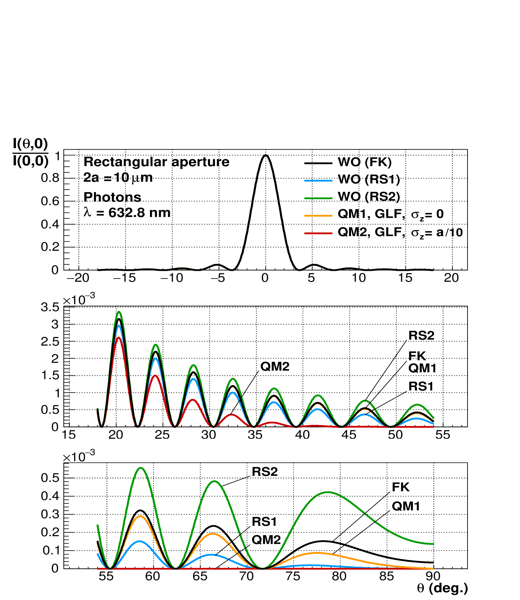
Figure 4: Comparison between different theoretical predictions of the relative intensity in Fraunhofer diffraction as a function of the diffraction angle in the horizontal plane for a rectangular slit of width $2a=10\;\mu$m and an incident monochromatic plane wave corresponding to photons of wavelength $\lambda=632.8$ nm (helium-neon laser). Five predictions are presented: three predictions of wave optics (WO) corresponding to the scalar theories of Fresnel-Kirchhoff (FK) and Rayleigh-Sommerfeld (RS1 and RS2) and two predictions of the quantum model (QM) corresponding to two values of the standard deviation $\sigma_{z}$ associated with a Gaussian longitudinal filtering (GLF) of the incident wave: $\sigma_{z}=0$ (QM1) and $\sigma_{z}=a/10$ (QM2). The values of the five intensities are distributed according to the decreasing order: RS2, FK, QM1, RS1, QM2, whatever $\theta$ is over the entire range 0^∘- 90^∘. These predictions correspond to the case where the polarization is not measured.

III.1.6 Large diffraction angles.

From the above analysis, it turns out that the relative gaps between the predictions of the different models considered here are significant at large angles. Moreover, from a survey of the literature, it seems that no accurate experimental study of the diffraction in this region has been carried out so far. Since the time when the FK and RS1-2 theories were formulated (late 19th century), technologies in optics have made tremendous progress due in particular to accurate measurements of intensity by charge-coupled devices which make it possible to achieve a sufficiently expanded dynamic range. An experimental study of this still little explored region is therefore probably feasible at the present time.

III.2 Polarization probabilities (photons)

From (​​ 37) and (​​ 124), the conditional probability to detect a photon of helicity $\xi$ if its momentum is $\hbar\mathbf{k}$ is:

$$\!\!P_{[\Sigma]_{\mathbf{K}}|\mathbf{K}=\mathbf{k}}^{({1})}\!\left([\xi]_{\mathbf{k}}\right)=\left|\!\,{}_{\mathbf{k}\!\!\!}\,\left<\,\!\xi\left|\,\chi^{({1})}_{\textup{out}}(\mathbf{k})\!\right.\right>\,\!\right|^{2}\!\!=\left|\!\,{}_{\mathbf{k}_{0}\!\!\!}\,\left<\,\!\xi\left|\,\!\chi^{({1})}_{\textup{in}}\right.\right>\,\!\right|^{2}\!\!.\hskip 21.33955pt$$ (190)

So the probabilities of the helicity states and consequently of the circular polarizations are conserved.

Note that for an aperture of sub-wavelength size, circular polarization probabilities are not conserved for all diffraction angles because the aperture limits the transmission of circularly polarized light [38]. This effect is not taken into account in assumption (​​ 17) and consequently the polarization predicted by the model does not match the experiment in this specific case.

For an elliptically polarized initial state $\left|\,\widetilde{\chi}^{({1})}_{\textup{in}}\;\right>\,$, with major axis azimuth $\zeta_{0}$, ellipticity angle $\eta_{0}$ and handedness $\xi_{0}$ (Eq. (​​ 133)), the conditional probabilities of linear polarization in the direction defined by the angle $\Psi$ with respect to the $x[\mathbf{k}]$ axis are expressed, from (​​ 136), by:

$$\!\!\begin{array}[]{l}\displaystyle P_{[X]_{\mathbf{K},\Psi}|\mathbf{K}=\mathbf{k}}^{({1})}\left([x]_{\mathbf{k},\Psi}\right)=\left|\;\,{}_{\!\!\mathbf{k},\Psi\!\!\!}\,\left<\,x\left|\,\widetilde{\chi}^{({1})}_{\textup{out}}(\mathbf{k})\right.\right>\,\right|^{2}\!\!\vspace{0.15cm}\\ \displaystyle\hskip 35.56593pt=\frac{1}{2}\left\{\,1+\cos 2\eta_{0}\cos 2[\,\zeta_{0}+\alpha_{3}(\mathbf{k})-\Psi\,]\,\right\},\end{array}\hskip 21.33955pt$$ (193)

whatever $\xi_{0}$, where $\alpha_{3}(\mathbf{k})$ is the rotation angle of the ellipse axes due to diffraction. From (​​ 193), we have:

$$\alpha_{3}(\mathbf{k})=\Psi\!-\!\zeta_{0}+\frac{1}{2}\arccos\frac{\,2\left|\,\,{}_{\!\!\mathbf{k},\Psi\!\!\!}\,\left<\,\!x\left|\,\widetilde{\chi}^{({1})}_{\textup{out}}(\mathbf{k})\!\right.\right>\,\right|^{2}\!\!-1\,}{\cos 2\eta_{0}},\hskip 21.33955pt$$ (194)

where $\mathbf{k}=\mathbf{k}(k,\theta,\phi)$. Therefore, the measurement of the probability $\left|\,\,{}_{\!\!\mathbf{k},\Psi\!\!\!}\,\left<\,x\left|\,\widetilde{\chi}^{({1})}_{\textup{out}}(\mathbf{k})\right.\right>\,\right|^{2}$ as a function of $k,\theta$, and $\phi$ makes it possible to fit the function $\alpha_{3}[\mathbf{k}(k,\theta,\phi)]$ to the experimental data (provided that $\eta_{0}\neq\pi/4$). From (​​ 4) and (​​ 117), its expected value is zero for $\theta=\phi=0$.

In the case of a linear polarization ($\eta_{0}=0$), the final polarization is also linear in the direction defined by the angle $\zeta_{0}+\alpha_{3}(\mathbf{k})$ [Eq. (​​ 139)]. Assuming that the maximum transmission axis of the analyzer is the axis $\mathcal{R}(0,0,\Psi)\,x[\mathbf{k}]$, the device can be rotated around $z[\mathbf{k}]$ so as to find the angle $\Psi_{1}(\mathbf{k})$ such that $\left|\,\,{}_{\!\!\mathbf{k},\Psi_{1}(\mathbf{k})\!\!\!}\,\left<\,\!x\left|\,\widetilde{\chi}^{({1})}_{\textup{out}}(\mathbf{k})\!\right.\right>\,\right|^{2}=1$. Then, (​​ 194) leads to: $\alpha_{3}(\mathbf{k})=\Psi_{1}(\mathbf{k})-\zeta_{0}$.

IV Conclusion

It is possible to construct a model based exclusively on quantum mechanics to describe the Fraunhofer diffraction by a diaphragm. In the model presented here, the quantum concept of measurement was used, within the framework of the S-matrix formalism, to describe the passage of the particles through the aperture. The notion of projector had to be generalized by that of filtering operator in order to obtain a description of the measurement compatible with the Huygens-Fresnel principle. Then, because of kinematics, it was necessary to assume that the passage of the particle through the aperture is described by a double measurement starting with the measurement of position (which creates a localized transitional state of indeterminate energy) and ending with an energy-momentum measurement (which creates the final state with the same energy as the initial state).

The model suggests that the wavelets involved in the Huygens-Fresnel principle are emitted from several neighboring wavefronts distributed along the longitudinal direction in the aperture region. These wavefronts contribute with different weights to the amplitude of the diffracted wave and the width of their distribution, not known a priori, can be fitted to the data from measurement of the intensity as a function of the diffraction angle. If this width is large enough, a significant damping of the intensity at large angles is predicted. A direct experimental study of the Huygens-Fresnel principle is therefore possible. Moreover, the model provides predictions concerning the still little explored region of large diffraction angles. In particular, it predicts the decrease in intensity towards zero at 90^∘, contrary to most of the scalar theories of wave optics. Finally, in the case of light in single-photon states and for an incident monochromatic plane wave, the model predicts that the transfer of momentum between the photon and the diaphragm conserves the probabilities of the circular polarizations but can cause a phase shift between the amplitudes of the associated helicity states. For an initial state elliptically polarized, the conservation of the ellipticity and of the handedness is predicted. The phase shift between the amplitudes of the helicity states corresponds to a rotation of the axes of the ellipse. The angle of this rotation depends on the diffraction angles and is not known a priori. Its values can be fitted to the data from measurements of the polarization of the photons detected beyond the diaphragm. It would thus be possible to get information on how diffraction modifies the polarization of light.

References

- [1]
- [2] P. S. Epstein and P. Ehrenfest, ”The quantum theory of the Fraunhofer diffraction”, Proc. Nat. Acad. Sci. 10, 133 (1924).
- [3] R. P. Feynman and A. R. Hibbs, Quantum Mechanics and Path Integrals (McGraw-Hill, New York, 1965), Chap. 3, Secs. 2-3.
- [4] A. O. Barut and S. Basri, ”Path integrals and quantum interference”, Am. J. Phys. 60, 896 (1992).
- [5] M. Beau, ”Feynman path integral approach to electron diffraction for one and two slits: analytical results”, Eur. J. Phys. 33, 1023 (2012).
- [6] C. Philippidis, C. Dewdney and B. J. Hiley, ”Quantum interference and the quantum potential”, Nuovo Cim. B 52, 15 (1979).
- [7] A. S. Sanz, F. Borondo and S. Miret-Artés, ”Particle diffraction studied using quantum trajectories”, J. Phys.: Condens. Matter 14, 6109 (2002).
- [8] X.-Y. Wu, B.-J. Zhang, J.-H. Yang, L.-X. Chi, X.-J. Liu, Y.-H. Wu, Q.-C. Wang, Y. Wang, J.-W. Li and Y.-Q. Guo, ”Quantum Theory of Light Diffraction”, J. Mod. Opt. 57(20), 2082 (2010).
- [9] C. Lupo, V. Giovannetti, S. Pirandola, S. Mancini and S. Lloyd, ”Capacities of linear quantum optical systems”, Phys. Rev. A 85, 062314 (2012).
- [10] J. Jung and O. Keller, ”Quantum-mechanical diffraction theory of light from a small hole: Extinction-theorem approach”, Phys. Rev. A 92, 012122 (2015).
- [11] Z. Xiao, R. N. Lanning, M. Zhang, I. Novikova, E. E. Mikhailov and J. P. Dowling, ”Why a hole is like a beam splitter: A general diffraction theory for multimode quantum states of light”, Phys. Rev. A 96, 023829 (2017).
- [12] S. Deepa, Bhargava Ram B.S. and P. Senthilkumaran. ”Helicity dependent diffraction by angular momentum transfer”. Sci. Rep. 9, 12491 (2019), doi:10.1038/s41598-019-48923-6.
- [13] T. V. Marcella, ”Quantum interference with slits”, Eur. J. Phys. 23, 615 (2002).
- [14] T. Rothman and S. Boughn, ”’Quantum interference with slits’ revisited”, Eur. J. Phys. 32, 107 (2011).
- [15] M.V. John and K. Mathew, ”Position Measurement-Induced Collapse: A Unified Quantum Description of Fraunhofer and Fresnel Diffractions”, Found. Phys. 49, 317 (2019).
- [16] L. D. Landau and E. M. Lifshitz, Relativistic Quantum Mechanics. (Pergamon, Oxford, 1960), §8, §16, §65.
- [17] M. Born and E. Wolf, Principles of Optics (Cambridge University Press, Cambridge, 1980), Chap. 8, Secs. 8.1-8.3, and 11.
- [18] A. Sommerfeld, Optics, Lectures on Theoretical Physics IV (Academic Press inc., NewYork, 1954), Chap. 5, Secs. 34,38.
- [19] L. D. Landau and E. M. Lifshitz, The Classical Theory of Fields (Pergamon, Oxford, 1962), §59-61.
- [20] W. Heisenberg, The Physical Principles of the Quantum Theory (University of Chicago Press, Chicago, 1930), Chap. II, §2a.
- [21] T. D. Newton and E. P. Wigner, ”Localized States for Elementary Systems”, Rev. Mod. Phys. 21(3), 400 (1949).
- [22] I. Bialynicki-Birula, ”On the wave function of the photon”, Acta Phys. Pol. 86, 97(1994).
- [23] J. E. Sipe, ”Photon wave functions”, Phys. Rev. A 52, 1875 (1995).
- [24] M. Hawton, ”Photon position operator with commuting components”, Phys. Rev. A 59, 954 (1999).
- [25] M. Hawton and W. E. Baylis, ”Photon position operators and localized bases”, Phys. Rev. A 64, 012101 (2001); ”Angular momentum and the geometrical gauge of localized photon states”, Phys. Rev. A 71, 033816 (2005).
- [26] B. J. Smith and M. G. Raymer, ”Photon wave functions, wave-packet quantization of light, and coherence theory”, New J. Phys. 9, 414 (2007).
- [27] D.C. Brody, ”Biorthogonal quantum mechanics”, J. Phys. A, Math. Theor. 47 035305 (2014).
- [28] M. Hawton and V. Debierre, ”Maxwell meets Reeh-Schlieder: The quantum mechanics of neutral bosons”, Phys. Lett. A 381, 1926 (2017).
- [29] H. Babaei and A. Mostafazadeh, ”Quantum mechanics of a photon”, J. Math. Phys. 58, 082302 (2017).
- [30] M. Hawton, ”Maxwell quantum mechanics”, Phys. Rev. A 100, 012122 (2019); ”Photon quantum mechanics in real Hilbert space”, Phys. Rev. A 104, 052211 (2021).
- [31] C. Cohen-Tannoudji, J. Dupont-Roc, G. Grynberg, Photons and Atoms: Introduction to Quantum Electrodynamics (Wiley, New York, 1997), Chaps. I, III, and V.
- [32] L. D. Landau and E. M. Lifshitz, Quantum Mechanics. Non-relativistic Theory (Pergamon, Oxford, 1965), §57.
- [33] A. Messiah, Quantum Mechanics (North Holland, Amsterdam, 1962), Vol. II, Chaps. XIII, XXI, and Appendix C.
- [34] M. Tanabashi et al. (Particle Data Group), Review of Particle Physics, Phys. Rev. D 98, 030001 (2018), Sec. 39.4.2.2, p. 537.
- [35] I. S. Gradshteyn and I. M. Ryzhik, Tables of Integrals, Series, and Products, 5th ed., edited by A. Jeffrey (Elsevier, Amsterdam, 1994), Sec. 3.896.4, p. 514.
- [36] A. Sommerfeld, ”Mathematische Theorie der Diffraction”, Math. Ann. 47, 317 (1896).
- [37] L. D. Landau and E. M. Lifshitz, Electrodynamics of Continuous Media, (Pergamon, Oxford, 1960), §75, problem 1. The application of Sommerfeld’s exact calculation to the case of a slit requires simplifying assumptions and leads to an approximate expression of the diffracted wave intensity. The result is the right-hand side of Eq. ( 187) multiplied by plus a term equal to . This additional term is never zero and increases in the range . It is negligible provided that is not too large (). See also J. B. Keller, ”Geometrical Theory of Diffraction”, J. Opt. Soc. Am. 52, 116 (1962).
- [38] D.J. Shin, A. Chavez-Pirson, and Y.H. Lee, ”Diffraction of circularly polarized light from near-field optical probes”, J. Microsc. 194, 353 (1999).
- [39]