New Approach to General Nonlinear Discrete-Time Stochastic $H_{\infty}$ Control

Abstract

In this paper, a new approach based on convex analysis is introduced to solve the $H_{\infty}$ problem for discrete-time nonlinear stochastic systems. A stochastic version of bounded real lemma is proved and the state feedback $H_{\infty}$ control is studied. Two examples are presented to show the effectiveness of our developed theory.

Key words: $H_{\infty}$ control, bounded real lemma, convex analysis, internal stability, external stability.

1 Introduction

$H_{\infty}$ theory was initially formulated by Zames [1] in the early 1980’s for linear time-invariant systems, where the $H_{\infty}$ norm, defined in the frequency-domain form for a stable transfer matrix, plays an important role in robust linear control design; see [2] and [3]. A breakthrough of the classical $H_{\infty}$ theory in [4] initiated the time-domain state-space approach in the $H_{\infty}$ study, and turned the $H_{\infty}$ controller design into solving two algebraic Riccati equations (AREs). After the appearance of [4], $H_{\infty}$ control theory has made a great progress in the 1990’s [5]. Up to now, $H_{\infty}$ control has been successfully applied to network control [6], synthetic biology design [7, 8], etc..

Instead of solving two Riccati equations or Riccati inequalities as in [4] , Gahinet and Apkarian[9] introduced the linear matrix inequality (LMI) approach to the $H_{\infty}$ controller design, which is more convenient due to the usage of LMI Toolbox. In the time-domain framework, the $H_{\infty}$ control theory is first extended to nonlinear deterministic systems expressed by ordinary differential equations(ODEs). For example, based on the solutions of Hamilton-Jacobi equations or inequalities, the state feedback $H_{\infty}$ control [10] and output feedback $H_{\infty}$ control [11], [12], were discussed, respectively. The reference [13] first systematically studied the stochastic $H_{\infty}$ control of linear Itô systems, where a stochastic bounded real lemma was obtained in terms of linear matrix inequalities (LMIs), and the dynamic output feedback $H_{\infty}$ problem was also discussed. At the same time, the state feedback $H_{\infty}$ control for linear time-invariant Itô systems with state-dependent noise was also discussed in [14] based on stochastic differential game. We refer the reader to the monograph [15] for the early development in the $H_{\infty}$ control theory of linear Itô systems. Except for the $H_{\infty}$ estimation, the extended Kalman filtering on stochastic Itô systems was also discussed in [16]. By means of completing the squares and stochastic dynamic programming, the state-feedback $H_{\infty}$ control and robust $H_{\infty}$ filtering were extensively investigated in [17] and [18] for affine stochastic Itô systems. It can be founded that starting from 1998, the stochastic $H_{\infty}$ control has become a popular research field [19], which has been extended to other stochastic systems such as Markovian jumps [20, 21, 22], Poisson jumps [23] and Lévy processes [24].

With the development of $H_{\infty}$ control theory of continuous-time Itô systems, the discrete-time $H_{\infty}$ control has also attracted considerable attention. For deterministic linear systems, Basar and Bernhard [2] have developed the discrete-time counterpart of the continuous-time $H_{\infty}$ design. Based on the dissipation inequality, differential game, and LaSalle’s invariance principle, Lin and Byrnes [25] developed the $H_{\infty}$ control theory for general nonlinear discrete-time deterministic systems. Bouhtouri, Hinrichsen and Pritchard [26] first studied the $H_{\infty}$-type control for discrete-time linear stochastic systems with multiplicative noise. The infinite horizon mixed $H_{2}/H_{\infty}$ control for discrete-time stochastic systems with state and disturbance dependent noise can be found in [27], which turned out that the mixed $H_{2}/H_{\infty}$ controller design is associated with the solvability of the four coupled matrix-valued equations. For the disturbance attenuation problem of linear discrete-time multiplicative noise systems with Markov jumps, we refer the reader to [28]. Berman and Shaked [29] first explored the general discrete-time stochastic $H_{\infty}$ control problem, and presented a bounded real lemma in terms Hamilton-Jacobi inequality, where the Hamilton-Jacobi inequality contains the supremum of some conditional mathematical expectation. As an application, for a class of discrete-time time-varying nonlinear stochastic systems with multiplicative noises, a relatively easily testing criterion was derived via taking the Lyapunov function to be a quadratic form. In [30], we considered the finite horizon $H_{\infty}$ control for the following affine nonlinear system

$$\left\{\begin{array}[]{l}x_{k+1}=f(x_{k})+g(x_{k})u_{k}+h(x_{k})v_{k}\\ \ \ \ \ \ \ \ \hskip 14.22636pt+[f_{1}(x_{k})+g_{1}(x_{k})u_{k}+h_{1}(x_{k})v_{k}]\omega_{k},\\ z_{k}=\left[\begin{array}[]{cc}m(x_{k})\\ u_{k}\end{array}\right],\ x_{0}\in{\cal R}^{n}.\end{array}\right.$$ (1)

The references [31] and [32] discussed the $H_{\infty}$ filtering design for some uncertain discrete-time affine nonlinear systems with time delays by means of Hamilton-Jacobi inequalities or matrix inequalities.

However, there are still some essential difficulties in nonlinear stochastic $H_{\infty}$ control design due to the following reasons:

$\bullet$ Even for affine nonlinear discrete-time multiplicative noise systems (a special class of nonlinear stochastic systems), in order to separate the control input $u$ from unknown exogenous disturbance $v$, the selection of the Lyapunov candidate function has to be a quadratic function, which often leads to conservative results [19].

$\bullet$ Because the Hamilton-Jacobi inequality depends on the supremum of a conditional mathematical expectation function (see (8) of [29]) or the mathematical expectation of the state trajectory (see (30) of [30]), which makes the given $H_{\infty}$ controller be not easily constructed. So the general discrete-time nonlinear stochastic $H_{\infty}$ theory merits further study, and new methods should be introduced in this field.

$\bullet$ Even for the affine nonlinear system (1), as said in [19], the completing the squares technique is no longer applicable except for special quadratic Lyapunov functions. Different from linear system case, the nonlinear discrete system cannot be iterated. In addition, different from Itô systems where an infinitesimal generator ${\cal L}V(x)$ can be used, how to give practical $H_{\infty}$ criteria for general nonlinear discrete-time stochastic systems which are not dependent on the mathematical expectation of the trajectory is a challenging problem.

This paper will make a contribution to the $H_{\infty}$ theory of general nonlinear discrete-time stochastic systems. It is well-known that the bounded real lemma plays a key role in the study of $H_{\infty}$ control, so we will first establish a bounded real lemma for the following discrete-time nonlinear stochastic state-disturbance system

$$\left\{\begin{array}[]{l}x_{k+1}=f(x_{k},\omega_{k})+g(x_{k},\omega_{k})v_{k},\\ z_{k}=\left[\begin{array}[]{l}m(x_{k})\\ m_{1}(x_{k})v_{k}\end{array}\right],x_{0}\in\mathbb{R}^{n},k=0,1,2,\cdots\end{array}\right.$$ (6)

where $f:\mathbb{R}^{n}\times\mathbb{R}^{d}\rightarrow\mathbb{R}^{n}$, $g:\mathbb{R}^{n}\times\mathbb{R}^{d}\rightarrow\mathbb{R}^{n\times n_{v}}$, $m:\mathbb{R}^{n}\rightarrow\mathbb{R}^{n_{m}}$ and $m_{1}:\mathbb{R}^{n}\rightarrow\mathbb{R}^{(n_{z}-n_{m})\times n_{v}}$ are measurable vector/matrix-valued functions. $x_{k}$ , $v_{k}$ and $z_{k}$ represent respectively the system state, external disturbance and the regulated output with appropriate dimensions. Throughout this paper, $\{\omega_{k}\}_{k\in\mathbb{N}}$ is a sequence of independent $d$-dimensional random variables with an identical distribution defined on the complete probability space $(\Omega,\mathscr{F},\mathbb{P})$, and the corresponding filtration is $\mathbb{F}=\{\mathscr{F}_{k}\}_{k\in\mathbb{N}}$, where $\mathscr{F}_{k}$ is the $\sigma$-field generated by $\omega_{0},\cdots,\omega_{k-1}$. Based on the obtained bounded real lemma, we pay our attention to the $H_{\infty}$ control of the following controlled system

$$\left\{\begin{array}[]{l}x_{k+1}=f(x_{k},u_{k},\omega_{k})+g(x_{k},\omega_{k})v_{k}\\ z_{k}=\left[\begin{array}[]{c}m(x_{k},u_{k})\\ m_{1}(x_{k})v_{k}\end{array}\right],x_{0}\in\mathbb{R}^{n},k=0,1,2,\cdots\end{array}\right.$$ (11)

where $f:\mathbb{R}^{n}\times\mathbb{R}^{n_{u}}\times\mathbb{R}^{d}\rightarrow\mathbb{R}^{n}$ and $m:\mathbb{R}^{n}\times\mathbb{R}^{n_{u}}\rightarrow\mathbb{R}^{n_{m}}$ are respectively measurable vector-valued functions. $\{u_{k},k=0,1,2,\cdots\}$ is the control input sequence. $\{v_{k},k=0,1,2,\cdots\}$ and $\{u_{k},k=0,1,2,\cdots\}$ are adapted sequences with respect to $\{\mathscr{F}_{k},k=0,1,2,\cdots\}$.

For affine systems with multiplicative noises, when using the method of completing the squares as used in [29], the usual conditions are supposed that $V(x)$ has the form of quadratics $V(x)=x^{T}Px$ or is twice differentiable which will be used in Taylor’s expansion, see [17] and [31]. The main purposes of those assumptions are to separate $v$ from other variables(eg.$x$ or $u$). The same difficulty which is always the main one, also exists in solving $H_{\infty}$ problems of stochastic nonlinear system (6) and (11). Concretely, for system (6), separating $v$ from $x$ is the key that will solve $H_{\infty}$ problems to obtain some important results such as well known bounded real lemmas; and for system (11), separating $v$ from $u$ and $x$ is also the key problem in designing $H_{\infty}$ controller. In order to overcome those difficulties of dividing-variables, we find that the following properties of convex function $V:\mathbb{R}^{n}\rightarrow\mathbb{R}$

$$V(\alpha x+(1-\alpha)y)\leq\alpha V(x)+(1-\alpha)V(y),\ \alpha\in[0,1],x,y\in\mathbb{R}^{n}$$

can be used in the analysis of $H_{\infty}$ control problems to separate $v$ from $x$ or $u$. Based on this idea, we introduce a convex method to discuss the $H_{\infty}$ control problems of system (6) and (11).

This paper is organized as follows: In section 2, the stability theory for discrete-time nonlinear systems and martingale properties are retrospected, which will be used in the discussion of $H_{\infty}$ control. In section 3, the internal stability and external stability for system (6) are discussed. Based on the convex properties of the auxiliary Lyapunov function, the bounded real lemma for system (6) is obtained. In section 4, the state-feedback $H_{\infty}$ control is discussed via the convex analysis method, and then the state-feedback $H_{\infty}$ controller is designed. In section 5, numerical simulations are given to show the validity of the obtained results.

Throughout this paper, we adopt the following notations:

$\mathbb{R}$: the set of all real numbers; $\mathbb{R}^{+}$: the set of all positive real numbers including $0$; $\mathbb{R}^{n}$: the $n$-dimensional real vector space with the norm

$$|x|=\sqrt{\sum\limits_{i=1}^{n}x_{i}^{2}}$$

for $x=(x_{1},\cdots,x_{n})^{T}\in\mathbb{R}^{n}$; $\mathbb{R}^{m\times n}$: the set of all real $m\times n$ matrices; $\mathbb{N}$: the set of all positive integers including $0$; $n_{v}$: the dimension of vector $v$; $\mathcal{S}^{n}(\mathbb{R})$: the set of all $n\times n$ symmetric matrices; $\mathcal{S}^{n}_{+}(\mathbb{R})$: the set of all real positive definite symmetric matrices; $\bar{\sigma}(Q)(\underline{\sigma}(Q))$: the maximum(minimum) eigenvalue of $Q\in\mathcal{S}^{n}(\mathbb{R})$; $P\geq 0$($P>0$): the symmetric matrix $P$ is positive semi-definite (definite); $L^{2}(\Omega,\mathscr{F}_{k};\mathbb{R}^{n_{v}})$: the $\mathscr{F}_{k}$-measurable second-order moment random variable space with the norm

$$\|\xi\|_{L^{2}_{\mathscr{F}_{k}}}=\sqrt{\mathbb{E}|\xi|^{2}}<\infty;$$

${l^{2}_{\infty}(\Omega,\mathscr{F},\mathbb{F};\mathbb{R}^{n_{v}})}$: the space of stochastic sequence $v=\{v_{k}\}_{k\in\mathbb{N}}$ with the norm

$$\|v\|_{l_{\infty}^{2}}=\sqrt{\mathbb{E}\big{[}\sum\limits_{k=0}^{\infty}|v_{k}|^{2}\big{]}}<\infty,$$

where $v_{k}\in L^{2}(\Omega,\mathscr{F}_{k};\mathbb{R}^{n_{v}})$, $k\in\mathbb{N}$.

2 Preliminaries

Throughout this paper, let $(\Omega,\mathscr{F},\mathbb{P})$ be a complete probability space and $\{\omega_{k}\}_{k\in\mathbb{N}}$ is an $\mathbb{R}^{d}$-valued independent random variable sequence. Denote $\mathcal{N}$ the event set that has zero probability. Let $\mathscr{F}_{k}$ the $\sigma$-field generated by $\omega_{0},\omega_{1},\cdots,\omega_{k-1}$, i.e.,

$$\begin{array}[]{l}\mathscr{F}_{k}=\sigma\{\omega_{0},\omega_{1},\cdots,\omega_{k-1}\}\vee\mathcal{N},k\in\mathbb{N}.\end{array}$$

and $\mathscr{F}_{0}=\{\emptyset,\Omega\}$($\emptyset$ is the empty set, $\Omega$ is the sample space). Obviously, $\mathscr{F}_{k-1}\subset\mathscr{F}_{k}$, and we set $\mathbb{F}=\{\mathscr{F}_{k}\}_{k\in\mathbb{N}}$. Now, we first review some results on the conditional expectation which will be used latter. The following lemma is the special case of Theorem 6.4 in [33].

Lemma 2.1.

If $\mathbb{R}^{d}$-valued random variable $\eta$ is independent of the $\sigma-$field $\mathscr{G}\subset\mathscr{F}$, and $\mathbb{R}^{n}-$valued random variable $\xi$ is $\mathscr{G}-$measurable, then, for every bounded function $f:\mathbb{R}^{n}\times\mathbb{R}^{d}\rightarrow\mathbb{R}$, there exists

$$\mathbb{E}[f(\xi,\eta)|\mathscr{G}]=\mathbb{E}[f(x,\eta)]_{x=\xi}\quad\mbox{\rm a.s.}$$

We firstly retrospect the stability theory for the following discrete-time stochastic system

$$\begin{array}[]{l}\left\{\begin{array}[]{l}x_{k+1}=F_{k}(x_{k},\omega_{k}),\\ x_{0}\in\mathbb{R}^{n},\end{array}\right.\end{array}$$ (12)

where $F_{k}:\mathbb{R}^{n}\times\mathbb{R}^{d}\rightarrow\mathbb{R}^{n}$ is a measurable function with $F_{k}(0,\cdot)\equiv 0$. From the definition of system (12), it is easy to see that the solution $x_{k}$ is $\mathscr{F}_{k}-$adapted. Denote $x(k;s,x)$ or $x_{k}^{s,x}$ the solution of (12) at time $k$ with the initial state $x\in\mathbb{R}^{n}$ starting at $s\in\mathbb{N}$, where $k\geq s$.

Definition 2.1.

The equilibrium solution $x_{k}\equiv 0$ of (12) is said to be

(1) almost surely asymptotically stable, if, for all $x_{0}\in\mathbb{R}^{n}$, $s\geq 0$

$$\mathbb{P}\bigg{\{}\lim\limits_{k\rightarrow\infty}x(k;s,x_{0})=0\bigg{\}}=1.$$ (13)

(2) asymptotically $p$-stable, if

$$\lim\limits_{k\rightarrow\infty}\mathbb{E}[|x(k;s,x_{0})|^{p}]=0;$$ (14)

The following lemma is the LaSalle-type theorem for the discrete-time stochastic system (12); see [34] for details.

Lemma 2.2.

Suppose $W:\mathbb{R}^{n}\rightarrow\mathbb{R}^{+}$ is a positive function and $V_{k}:\mathbb{R}^{n}\rightarrow\mathbb{R}^{+}$, $k\in\mathbb{N}$, are the Lyapunov functions satisfying

$$\begin{array}[]{l}\mathbb{E}[V_{k+1}(F_{k}(x,\omega_{k}))]-V_{k}(x)\leq\gamma_{k}-W(x),\quad\forall x\in\mathbb{R}^{n},k\in\mathbb{N},\end{array}$$ (15)

$$\sum\limits_{k=0}^{\infty}\gamma_{k}<\infty$$

and

$$\begin{array}[]{l}\liminf\limits_{|x|\rightarrow\infty}\inf\limits_{k\in\mathbb{N}}V_{k}(x)=\infty.\end{array}$$ (16)

$\{x_{k}\}_{k\in\mathbb{N}}$ is the solution sequence of (12). Then

$$\lim\limits_{k\rightarrow\infty}V_{k}(x_{k})\quad\mbox{exists and is finite almost surely,}$$

and

$$\lim\limits_{k\rightarrow\infty}W(x_{k})=0\quad a.s..$$

Under the condition that $W$ is proper and continuous positive definite, the following corollary can be obtained directly by LaSalle-type theorem.

Corollary 2.1.

Suppose there exist a proper and continuous positive definite function $W$ and a Lyapunov function sequence $\{V_{k},k\in\mathbb{N}\}$ satisfying the conditions of Lemma 2.2, then

$$\lim\limits_{k\rightarrow\infty}x_{k}=0\quad\mbox{a.s..}$$

3 A discrete-time version of the bounded real lemma

Now we consider the discrete-time system (6), where $x(\cdot):=\{x_{k}\}_{k\in\mathbb{N}}$ is the solution of (6) with the initial state $x_{0}\in\mathbb{R}^{n}$, $v(\cdot):=\{v_{k}\}_{k\in\mathbb{N}}\in{l^{2}_{\infty}(\Omega,\mathscr{F},\mathbb{F};\mathbb{R}^{n_{v}})}$ is the exogenous disturbances to be rejected, and $z(\cdot):=\{z_{k}\}_{k\in\mathbb{N}}$ is the regulated output. Without loss of generality, we also assume that $0$ is the equilibrium of $f$ and $m$, i.e., $f(0,\cdot)\equiv 0,m(0)=0$. In this section, we denote $x(k;s,x_{s},v)$ or $x_{k}^{s,x_{s},v}$ the solution of (6) with the initial state $x_{s}\in\mathbb{R}^{n}$ and external disturbance $v(\cdot)$ starting at $s\in\mathbb{N}$, and denote the controlled output as $z(k;s,x_{s},v)$ or $z_{k}^{s,x_{s},v}$ corresponding to $x_{k}^{s,x_{s},v}$ for $k\geq s$. Throughout the paper, we assume that all random variables such as $V(x_{k})$ and $V_{k}(x_{k})$ are elements in $L^{1}(\Omega,\mathscr{F},\mathbb{P})$, i.e., $\mathbb{E}[V(x_{k})]<\infty$ and $\mathbb{E}[V_{k}(x_{k})]<\infty$.

Definition 3.1.

The system (6) is called internally stable if there exists $c>0$ such that

$$\sum\limits_{k=0}^{\infty}\mathbb{E}|z_{k}^{0,x_{0},0}|^{2}\leq c|x_{0}|^{2},\ \ x_{0}\in\mathbb{R}^{n},$$

where $z_{k}^{0,x_{0},0}=m(x_{k}^{0,x_{0},0})$.

For every positive function $V:\mathbb{R}^{n}\rightarrow\mathbb{R}^{+}$ and disturbance $v\in\mathbb{R}^{n_{v}}$, we define the difference operator $\Delta_{v}$ of system (6) as

$$\Delta_{v}V(x):=\mathbb{E}[V(f(x,\omega_{k})+g(x,\omega_{k})v)]-V(x),x\in\mathbb{R}^{n}.$$

Because we assume that $\{\omega_{k}\}_{k\in\mathbb{N}}$ is independently identically distributed, so

$$\mathbb{E}[V(f(x,\omega_{k})+g(x,\omega_{k})v)]=\mathbb{E}[V(f(x,\omega_{k+1})+g(x,\omega_{k+1})v)],$$

i.e., the difference operator $\Delta_{v}$ is identical for all $k\in\mathbb{N}$. Specially, for $v(\cdot)\equiv 0$, the operator $\Delta_{0}$ reduces to

$$\Delta_{0}V(x):=\mathbb{E}[V(f(x,\omega_{k}))]-V(x),x\in\mathbb{R}^{n}.$$

Lemma 3.1.

Suppose there exist a positive function $V:\mathbb{R}^{n}\rightarrow\mathbb{R}^{+}$, and two positive constants $c_{1}>0$ and $c_{2}>0$, such that

$$\Delta_{0}V(x)\leq-c_{1}|m(x)|^{2},$$ (17)

$$V(x)\leq c_{2}|x|^{2},$$ (18)

then system (6) is internally stable. Moreover, if $|m(x)|$ is positive definite, then for every $x_{0}\in\mathbb{R}^{n}$, we have

$$\lim\limits_{k\rightarrow\infty}x_{k}^{0,x_{0},0}=0\quad\mbox{a.s..}$$ (19)

Proof.

Since

$$\mathbb{E}[V(x_{k+1})]-\mathbb{E}[V(x_{k})]=\mathbb{E}\bigg{[}\mathbb{E}\big{[}V(f(x_{k},\omega_{k}))|\mathscr{F}_{k}\big{]}-V(x_{k})\bigg{]},$$

$x_{k}$ is $\mathscr{F}_{k}$-measurable and $\omega_{k}$ is independent of $\mathscr{F}_{k}$, by Lemma 2.1, we have

$$\mathbb{E}[V(x_{k+1})]-\mathbb{E}[V(x_{k})] = \mathbb{E}\bigg{\{}\bigg{[}\mathbb{E}[V(f(x,\omega_{k}))]-V(x)\bigg{]}_{x=x_{k}}\bigg{\}}$$

$$= \mathbb{E}\big{[}\Delta_{0}V(x_{k})\big{]}.$$

By condition (17), it shows that

$$\mathbb{E}[V(x_{k+1})]-\mathbb{E}[V(x_{k})]\leq-c_{1}\mathbb{E}|m(x_{k})|^{2}.$$

For every $N\in\mathbb{N}$, taking the summation on both sides of the above inequality for $k$ from $0$ to $N$, we obtain that

$$\mathbb{E}[V(x_{N+1})]-\mathbb{E}[V(x_{0})]\leq-c_{1}\sum\limits_{k=0}^{N}\mathbb{E}|m(x_{k})|^{2}.$$

Since $V(x)$ is a positive function, the above inequality yields

$$\sum\limits_{k=0}^{N}\mathbb{E}|m(x_{k})|^{2}\leq\frac{1}{c_{1}}\mathbb{E}[V(x_{0})].$$ (20)

In view of (18), by letting $N\rightarrow\infty$ on the left-hand side of (20), we have

$$\sum\limits_{k=0}^{\infty}\mathbb{E}|m(x_{k})|^{2}\leq\frac{1}{c_{1}}V(x_{0})\leq\frac{c_{2}}{c_{1}}|x_{0}|^{2}.$$ (21)

Since $|z_{k}^{0,x_{0},0}|=|m(x_{k})|$, the internal stability is shown from (21).

As far as (19), it can be obtained directly by Lemma 2.2 and the positive definiteness of the function $W(x)=c_{1}|m(x)|^{2}$. ∎

Now, we will show the converse of Lemma 3.1 which is characterized by the following lemma.

Lemma 3.2.

Suppose system (6) is internally stable. Then there exists a positive function $V:\mathbb{R}^{n}\rightarrow\mathbb{R}^{+}$ satisfying (17) and (18).

Proof.

For every $x\in\mathbb{R}^{n}$, define

$$V_{k}(x)=\sum\limits_{i=k}^{\infty}\mathbb{E}|m(x^{k,x,0}_{i})|^{2}.$$ (22)

Because, for every $k\in\mathbb{N}$, the following fact holds:

$$x_{k+1}^{k,x,0}=f(x,\omega_{k}),$$

which implies that

$$x_{i}^{k,x,0}=x_{i}^{k+1,x_{k+1}^{k,x,0},0}=x_{i}^{k+1,f(x,\omega_{k}),0},\quad i>k.$$

Using the above property for the solution of system (6), we have

$$\mathbb{E}[V_{k+1}(f(x,\omega_{k}))]-V_{k}(x) = \mathbb{E}\left\{\left[\sum\limits_{i=k+1}^{\infty}\mathbb{E}|m(x^{k+1,y,0}_{i})|^{2}\right]_{y=f(x,\omega_{k})}\right\}$$

$$-\sum\limits_{i=k}^{\infty}\mathbb{E}|m(x^{k,x,0}_{i})|^{2}$$

$$= \sum\limits_{i=k+1}^{\infty}\mathbb{E}|m(x^{k,x,0}_{i})|^{2}-\sum\limits_{i=k}^{\infty}\mathbb{E}|m(x^{k,x,0}_{i})|^{2}$$

$$= -\mathbb{E}|m(x^{k,x,0}_{k})|^{2}=-|m(x)|^{2}.$$

Hence, we obtain the following equations for all $k\in\mathbb{N}$:

$$\mathbb{E}[V_{k+1}(f(x,\omega_{k}))]-V_{k}(x)=-|m(x)|^{2},\ k\in\mathbb{N}.$$ (23)

Below, we prove that for any $k\in\mathbb{N}$, the following holds:

$$V_{k}(x)=V_{k+1}(x),\ \ x\in\mathbb{R}^{n}.$$

Because, for every $k\in\mathbb{N}$, $x_{k+1}^{k,x,0}=f(x,\omega_{k})$, $x_{k+2}^{k+1,x,0}=f(x,\omega_{k+1})$, and $\omega_{k}$ and $\omega_{k+1}$ are independently identically distributed, which implies that $x_{k+1}^{k,x,0}$ and $x_{k+2}^{k+1,x,0}$ are also identically distributed. So

$$\mathbb{E}|m(x_{k+1}^{k,x,0})|^{2}=\mathbb{E}|m(x_{k+2}^{k+1,x,0})|^{2}.$$

Similarly, the following relationship holds:

$$\mathbb{E}|m(x_{i}^{k,x,0})|^{2}=\mathbb{E}|m(x_{i+1}^{k+1,x,0})|^{2},\ i=k,k+1,\cdots$$

By the definition of $V(x)$ in (22), we have

$$V_{k}(x)=V_{k+1}(x),\ \forall k\in\mathbb{N},$$

which implies that $V_{k}(x)$ is identical for all $k\in\mathbb{N}$. Therefore, if we let

$$V(x)=\sum\limits_{i=0}^{\infty}\mathbb{E}|m(x^{0,x,0}_{i})|^{2},$$ (24)

then, by the above discussion, it follows that $V(x)=V_{k}(x),\forall k\in\mathbb{N}$. As so, the equation (23) reduces to

$$\Delta_{0}V(x)=-|m(x)|^{2}.$$ (25)

Taking $c_{1}=1$, we have proved that $V$ defined by (24) satisfies (17).

As far as $V(x)$ satisfies (18), it can be obtained directly by the internal stability of system (6) and Definition 3.1. ∎

By the equations (24) and (25), we have the following corollary.

Corollary 3.1.

Suppose system (6) is internally stable. Then there exists a positive function $V:\mathbb{R}^{n}\rightarrow\mathbb{R}^{+}$ satisfying (25). Moreover, there also exists

$$V(x)\geq|m(x)|^{2}.$$ (26)

Proof.

Obviously, it only remains to show that (26). By definition of $V(x)$ in (24), we have

$$V(x)\geq|m(x_{0}^{0,x,0})|^{2}.$$

In view of the fact that $m(x_{0}^{0,x,0})=m(x)$, (26) is hence proved. ∎

Combining Lemma 3.1 and Lemma 3.2, the following proposition 3.1 is obtained, which presents a necessary and sufficient condition of the internal stability of system (6). Denote

$$\mathcal{H}_{0}(V(x)):=\mathbb{E}[V(f(x,\omega_{0}))]-V(x)+|m(x)|^{2}.$$ (27)

Proposition 3.1.

System (6) is internally stable if and only if there exist a positive function $V:\mathbb{R}^{n}\rightarrow\mathbb{R}^{+}$ and a positive constant $c_{2}>0$ such that

$$V(x)\leq c_{2}|x|^{2},\ \ \forall x\in\mathbb{R}^{n},$$ (28)

$$\mathcal{H}_{0}(V(x))\leq 0,\ \ \forall x\in\mathbb{R}^{n}.$$ (29)

Definition 3.2.

The system (6) is said to be externally stable or $l^{2}$-input-output stable if, for every $v(\cdot)\in{l^{2}_{\infty}(\Omega,\mathscr{F},\mathbb{F};\mathbb{R}^{n_{v}})}$,

$$z(\cdot)=\{z_{k}^{0,0,v}\}_{k\in\mathbb{N}}\in{l^{2}_{\infty}(\Omega,\mathscr{F},\mathbb{F};\mathbb{R}^{n_{z}})},$$

and there exists a positive real number $\gamma>0$ such that

$$\|z(\cdot)\|_{l^{2}_{\infty}}\leq\gamma\|v(\cdot)\|_{l^{2}_{\infty}},\forall v(\cdot)\in{l^{2}_{\infty}(\Omega,\mathscr{F},\mathbb{F};\mathbb{R}^{n_{v}})},$$

or equivalently,

$$\sum\limits_{k=0}^{\infty}\mathbb{E}[|z_{k}^{0,0,v}|^{2}]\leq\gamma^{2}\sum\limits_{k=0}^{\infty}\mathbb{E}[|v_{k}|^{2}].$$ (30)

Remark 3.1.

Suppose $\gamma$ is a given positive real number. If inequality (3.2) or (30) holds, system (6) is also said to have $l_{2}$-gain less than or equal to $\gamma$ [25]. Moreover, suppose that system (6) is externally stable. Define an operator

$$\mathcal{L}:{l^{2}_{\infty}(\Omega,\mathscr{F},\mathbb{F};\mathbb{R}^{n_{v}})}\rightarrow{l^{2}_{\infty}(\Omega,\mathscr{F},\mathbb{F};\mathbb{R}^{n_{z}})}$$

by

$$\mathcal{L}(v)=z(\cdot,0,0,v),v\in{l^{2}_{\infty}(\Omega,\mathscr{F},\mathbb{F};\mathbb{R}^{n_{v}})},$$

then operator $\mathcal{L}$ is called the perturbation operator of (6). Its norm is defined as

$$\|\mathcal{L}\|=\sup\limits_{0\neq v(\cdot)\in{l^{2}_{\infty}(\Omega,\mathscr{F},\mathbb{F};\mathbb{R}^{n_{v}})}}\frac{\|z(\cdot,0,0,v)\|_{{l^{2}_{\infty}(\Omega,\mathscr{F},\mathbb{F};\mathbb{R}^{n_{z}})}}}{\|v\|_{{l^{2}_{\infty}(\Omega,\mathscr{F},\mathbb{F};\mathbb{R}^{n_{v}})}}}.$$ (31)

So, on one hand, $\|\mathcal{L}\|$ is a measure of the $l_{2}$-gain of system (6), but on the other hand, it is also a measure of the worst case effect that the stochastic disturbance $v$ may have on the controlled output $z$. Therefore, it is important to find a way to determine or estimate the norm $\|\mathcal{L}\|$.

Proposition 3.2.

Suppose, for $\gamma>0$, there exist a convex positive function $V:\mathbb{R}^{n}\rightarrow\mathbb{R}^{+}$ and a real number $\beta>1$, such that

$$\mathcal{H}_{1}(V(x),\beta):=\frac{1}{\beta}\mathbb{E}[V(\beta f(x,\omega_{0}))]-V(x)+|m(x)|^{2}\leq 0,$$ (32)

$$G_{\beta}(V(x))\leq\gamma^{2},\forall x\in\mathbb{R}^{n},V(0)=0,$$ (33)

where $G_{\beta}(V(x))$ is defined by

$$G_{\beta}(V(x)):=\sup\limits_{0\neq v\in\mathbb{R}^{n_{u}}}\left\{\frac{(\beta-1)}{\beta}\frac{\mathbb{E}\big{[}V(\frac{\beta}{\beta-1}g(x,\omega_{0})v)\big{]}}{|v|^{2}}+\frac{|m_{1}(x)v|^{2}}{|v|^{2}}\right\}.$$ (34)

Then $\|\mathcal{L}\|\leq\gamma$. Moreover, if $V$ satisfies (18), then system (6) is also internally stable.

Proof.

Let $\alpha=1/\beta$, then $0<\alpha<1$. By the convexity of $V$, it follows

$$\Delta_{v}V(x) = \mathbb{E}[V(f(x,\omega_{k})+g(x,\omega_{k})v)]-V(x)$$

$$=\mathbb{E}\bigg{[}V(\alpha\frac{1}{\alpha}f(x,\omega_{k})+(1-\alpha)\frac{1}{1-\alpha}g(x,\omega_{k})v)\bigg{]}-V(x)$$

$$\leq\alpha\mathbb{E}\bigg{[}V(\frac{1}{\alpha}f(x,\omega_{k}))\bigg{]}+(1-\alpha)\mathbb{E}\bigg{[}V(\frac{1}{1-\alpha}g(x,\omega_{k})v)\bigg{]}$$

$$\quad-V(x)+|m(x)|^{2}-\gamma^{2}|v|^{2}-|m(x)|^{2}+\gamma^{2}|v|^{2}.$$

$$\leq\mathcal{H}_{1}(V(x),\beta)+[G_{\beta}(V(x))-\gamma^{2}]|v|^{2}-|z|^{2}+\gamma^{2}|v|^{2}.$$

By conditions of (32) and (33), it follows that

$$\Delta_{v}V(x)\leq-|z|^{2}+\gamma^{2}|v|^{2}.$$

Denote $x_{k}$ the solution of (6) with initial state $x_{0}=0$ for $v(\cdot)\in{l^{2}_{\infty}(\Omega,\mathscr{F},\mathbb{F};\mathbb{R}^{n_{v}})}$, $z_{k}$ is the corresponding output. Then, we have

$$\left\{\mathbb{E}[V(f(x,\omega_{k})+g(x,\omega_{k})v)]-V(x)\right\}_{x=x_{k},v=v_{k}}\leq-|z_{k}|^{2}+\gamma^{2}|v_{k}|^{2},$$

Since $x_{k}$ and $v_{k}$ are $\mathscr{F}_{k}$-measurable, by Lemma 2.1, the above inequality can also be written as

$$\mathbb{E}[V(f(x_{k},\omega_{k})+g(x_{k},\omega_{k})v_{k})|\mathscr{F}_{k}]-V(x_{k})\leq-|z_{k}|^{2}+\gamma^{2}|v_{k}|^{2},$$

i.e.

$$\mathbb{E}[V(x_{k+1})|\mathscr{F}_{k}]-V(x_{k})\leq-|z_{k}|^{2}+\gamma^{2}|v_{k}|^{2},$$

Taking the mathematical expectation on both sides of the above inequality, we have

$$\mathbb{E}[V(x_{k+1})]-\mathbb{E}[V(x_{k})]\leq-\mathbb{E}[|z_{k}|^{2}]+\gamma^{2}\mathbb{E}[|v_{k}|^{2}].$$ (35)

For every $N\in\mathbb{N}$, taking a summation on both sides of (35) from $k=0$ to $k=N$, we have

$$\mathbb{E}[V(x_{N+1})]-\mathbb{E}[V(x_{0})]\leq-\sum\limits_{k=0}^{N}\mathbb{E}[|z_{k}|^{2}]+\gamma^{2}\sum\limits_{k=0}^{N}\mathbb{E}[|v_{k}|^{2}].$$

Since $V(x_{0})=V(0)=0$, and $V(x)\geq 0$, we obtain that

$$\sum\limits_{k=0}^{N}\mathbb{E}[|z_{k}|^{2}]\leq\gamma^{2}\sum\limits_{k=0}^{N}\mathbb{E}[|v_{k}|^{2}].$$

Let $N\rightarrow\infty$, we get

$$\sum\limits_{k=0}^{\infty}\mathbb{E}[|z_{k}|^{2}]\leq\gamma^{2}\sum\limits_{k=0}^{\infty}\mathbb{E}[|v_{k}|^{2}].$$

This proves that (6) is externally stable and $\|\mathcal{L}\|\leq\gamma$.

Now, we will prove that system (6) is also internally stable. Since

$$V(x) = V(\alpha\beta x+(1-\alpha)0)\leq\alpha V(\beta x)+(1-\alpha)V(0)$$

$$= \alpha V(\beta x),$$

this implies

$$V(\beta x)\geq\beta V(x).$$

By (32) and above inequality, we obtain

$$\mathbb{E}[V(f(x,\omega_{0}))]-V(x)+|m(x)|^{2}\leq 0,$$

i.e.

$$\mathcal{H}_{0}(V(x))\leq 0.$$

By Proposition 3.1, we proves that system (6) is internally stable. ∎

Remark 3.2.

Denote ${\mathbb{V}}$ a set of all positive convex functions defined on $\mathbb{R}^{n}$ satisfying (18) and

$${\mathscr{B}_{\mathbb{V}}}=\left\{\begin{array}[]{r}(\beta,V):\beta>1\mbox{ and }V\in{\mathbb{V}}\mbox{ satisfy \eqref{eq-H-1-ineq-1}}\end{array}\right\}.$$

Define

$$\gamma^{*^{2}}=\inf\limits_{(\beta,V)\in{\mathscr{B}_{\mathbb{V}}}}\sup\limits_{x\in\mathbb{R}^{n}}G_{\beta}(V(x)).$$ (37)

From the proof of Proposition 3.2, we can see that $\|\mathcal{L}\|\leq\gamma^{*}$. This can be used to estimate the upper bound of operator norm $\|\mathcal{L}\|$, though $\gamma^{*}$ given by (37) is not necessarily the best one. But it is the locally best one, this is because that $V$ is confined to ${\mathbb{V}}$ which is a subset of convex functions.

In order to induce the bounded real lemma for system (6), we introduce the definition of convexity of vector-valued function as following.

Definition 3.3.

Let $f_{0}:\mathbb{R}^{n}\rightarrow\mathbb{R}^{n_{0}}$ and $h:\mathbb{R}^{n_{0}}\rightarrow\mathbb{R}$. The vector-valued function $f_{0}$ is said convex with respect to $h$, or is called $h-$convex if the compound function $h\circ f_{0}:\mathbb{R}^{n}\rightarrow\mathbb{R}$ is convex, i.e., for every $0<\alpha<1$ and $x,y\in\mathbb{R}^{n}$, there exists

$$h(f_{0}(\alpha x+(1-\alpha)y))\leq\alpha h(f_{0}(x))+(1-\alpha)h(f_{0}(y)).$$ (38)

Remark 3.3.

The definition of $h-$convexity can be seen as an extension of logarithmic convexity used in [35].

In this paper, the following assumption is needed and will be used in the latter discussion.

($A_{1}$): For every $w\in\mathbb{R}^{d}$, $m(\cdot):\mathbb{R}^{n}\rightarrow\mathbb{R}^{n_{m}}$ and $m\circ f(\cdot,w):\mathbb{R}^{n}\rightarrow\mathbb{R}^{n_{m}}$ are $h-$convex, where $h:\mathbb{R}^{n_{m}}\rightarrow\mathbb{R}$ is defined by $h(y)=|y|^{2},y\in\mathbb{R}^{n_{m}}$.

Lemma 3.3.

Suppose Assumption ($A_{1}$) holds and system (6) is internally stable. Then $V:\mathbb{R}^{n}\rightarrow\mathbb{R}^{+}$ defined by (24) is a convex function.

Proof.

Let $x_{i}^{0,x,0}$ the solution of system (6) starting at $k=0$ with initial state $x\in\mathbb{R}^{n}$ for $v(\cdot)=0$. Since, for every $0<\alpha<1$ and $x,y\in\mathbb{R}^{n}$

$$x^{0,\alpha x+(1-\alpha)y,0}_{0}=\alpha x+(1-\alpha)y,$$

applying the $h-$convexity of $m(\cdot)$ and $m\circ f$, we have

$$|m(x^{0,\alpha x+(1-\alpha)y,0}_{0})|^{2} = |m(\alpha x+(1-\alpha)y)|^{2}\leq\alpha|m(x)|^{2}+(1-\alpha)|m(y)|^{2}$$

$$= \alpha|m(x^{0,x,0}_{0})|^{2}+(1-\alpha)|m(x^{0,y,0}_{0})|^{2},$$

and

$$|m(f(x^{0,\alpha x+(1-\alpha)y,0}_{0}))|^{2}\leq\alpha|m(f(x^{0,x,0}_{0}))|^{2}+(1-\alpha)|m(f(x^{0,y,0}_{0}))|^{2}.$$

Now we use the inductive method to prove that, for all $k\in\mathbb{N}$, the following two inequalities are true:

$$\mathbb{E}[|m(x^{0,\alpha x+(1-\alpha)y,0}_{k})|^{2}]\leq\alpha\mathbb{E}[|m(x^{0,x,0}_{k})|^{2}]+(1-\alpha)\mathbb{E}[|m(x^{0,y,0}_{k})|^{2}]$$

and

$$\mathbb{E}[|m(f(x^{0,\alpha x+(1-\alpha)y,0}_{k}))|^{2}]\leq\alpha\mathbb{E}[|m(f(x^{0,x,0}_{k}))|^{2}]+(1-\alpha)\mathbb{E}[|m(f(x^{0,y,0}_{k}))|^{2}].$$ (39)

Firstly, for $k=0$, by the just above discussions, we see that (3) and (39) are true.

Suppose, for $k\leq i$, the inequalities of (3) and (39) are true. Then, for $k=i+1$, keeping $m\circ f$ is $h-$convex in mind, we have

$$\mathbb{E}[|m(x^{0,\alpha x+(1-\alpha)y,0}_{i+1})|^{2}] = \mathbb{E}[|m(f(x^{0,\alpha x+(1-\alpha)y,0}_{i},\omega_{i}))|^{2}]$$

$$\leq \alpha\mathbb{E}[|m(f(x^{0,x,0}_{i},\omega_{i}))|^{2}]+(1-\alpha)\mathbb{E}[|m(f(x^{0,y,0}_{i},\omega_{i}))|^{2}]$$

$$\leq \alpha\mathbb{E}[|m(x^{0,x,0}_{i+1})|^{2}]+(1-\alpha)\mathbb{E}[|m(x^{0,y,0}_{i+1})|^{2}].$$

Similarly, we can prove that (39) is true for $k=i+1$. By induction, we prove that (3) and (39) are true.

For every $N\in\mathbb{N}$, taking summation on both sides of (3) for $k$ from $0$ to $N$, we obtain

$$\sum\limits_{k=0}^{N}\mathbb{E}[|m(x^{0,\alpha x+(1-\alpha)y,0}_{k})|^{2}]\leq\alpha\sum\limits_{k=0}^{N}\mathbb{E}[|m(x^{0,x,0}_{k})|^{2}]+(1-\alpha)\sum\limits_{k=0}^{N}\mathbb{E}[|m(x^{0,y,0}_{k})|^{2}].$$

Since system (6) is internally stable, together with definition of $V(x)$ by (24), when let $N\rightarrow\infty$, we get

$$V(\alpha x+(1-\alpha)y)\leq\alpha V(x)+(1-\alpha)V(y),$$

which shows that $V(x)$ is convex. This ends the proof. ∎

We now will show that under some proper conditions, an internally stable system (6) is also externally stable. In the rest of this section, the following assumptions are needed.

($A_{2}$): $m_{1}(x)$ and $\mathbb{E}[g(x,\omega_{k})^{T}g(x,\omega_{k})]$ are bounded.

($A_{3}$): For internally stable system (6), there exist two continuous positive functions $C_{1},C_{2}:\mathbb{R}^{+}\rightarrow\mathbb{R}^{+}$ with $C_{1}(1)<1$ such that

$$C_{2}(\beta)\bar{V}(x)\leq\mathbb{E}[\bar{V}(\beta f(x,\omega_{k}))]\leq C_{1}(\beta)\bar{V}(x),$$ (40)

where $\bar{V}:\mathbb{R}^{n}\rightarrow\mathbb{R}^{+}$ is defined by Lemma 3.1.

Lemma 3.4.

Under Assumptions ($A_{1}$), ($A_{2}$) and ($A_{3}$), suppose system (6) is internally stable, then (6) is externally stable. Moreover, there exist $\gamma>0$ and a positive function $V:\mathbb{R}^{n}\rightarrow\mathbb{R}^{+}$ such that (32) and (33) hold.

Proof.

Since system (6) is internally stable, by Lemma 3.1, take $\bar{V}$ defined by (24), then

$$\Delta_{0}\bar{V}(x)\leq-|m(x)|^{2},$$

i.e.,

$$\mathbb{E}[\bar{V}(f(x,\omega_{k}))]-\bar{V}(x)+|m(x)|^{2}\leq 0.$$ (41)

By Assumption ($A_{3}$), $C_{1}(\cdot)$ is continuous and $C_{1}(1)<1$, so

$$\lim\limits_{\beta\rightarrow+1}(\beta-C_{1}(\beta))=1-C_{1}(1)>0.$$

This implies that there exits $\beta_{0}>1$ such that

$$\beta_{0}-C_{1}(\beta_{0})>0.$$ (42)

Taking

$$q_{0}=\frac{C_{1}(\beta_{0})(1-C_{2}(1))}{\beta_{0}-C_{1}(\beta_{0})},\ \ p_{0}=\frac{q_{0}\beta_{0}}{C_{1}(\beta_{0})},$$ (43)

it is easy to check $p_{0}>q_{0}>0$. Let

$$V(x)=p_{0}\bar{V}(x).$$

Applying (40) in Assumption ($A_{3}$), we have

$$\mathbb{E}[\bar{V}(f(x,\omega_{k}))]-\bar{V}(x) \geq (C_{2}(1)-1)\bar{V}(x)=q_{0}\bar{V}(x)-p_{0}\bar{V}(x)$$

$$\geq \frac{q_{0}}{C_{1}(\beta_{0})}\mathbb{E}[\bar{V}(\beta_{0}f(x,\omega_{k}))]-p_{0}\bar{V}(x)$$

$$= \frac{1}{\beta_{0}}\frac{q_{0}\beta_{0}}{C_{1}(\beta_{0})}\mathbb{E}[\bar{V}(\beta_{0}f(x,\omega_{k}))]-p_{0}\bar{V}(x)$$

$$= \frac{1}{\beta_{0}}\mathbb{E}[p_{0}\bar{V}(\beta_{0}f(x,\omega_{k}))]-p_{0}\bar{V}(x)$$

$$= \frac{1}{\beta_{0}}\mathbb{E}[V(\beta_{0}f(x,\omega_{k}))]-V(x).$$

Keeping inequality (41) in mind, we obtain

$$\frac{1}{\beta_{0}}\mathbb{E}[V(\beta_{0}f(x,\omega_{k}))]-V(x)+|m(x)|^{2}\leq 0.$$

This proves that $V(x)=p_{0}\bar{V}(x)$ satisfies (32).

Now, we prove that $V(x)$ also satisfies (33). By Assumption ($A_{2}$), we have

$$\sigma_{\max,g}=\sup\limits_{x\in\mathbb{R}^{n}}\bar{\sigma}\big{(}\mathbb{E}\big{[}g(x,\omega_{k})^{T}g(x,\omega_{k})\big{]}\big{)}<\infty,$$

$$\sigma_{\max,m_{1}}=\sup\limits_{x\in\mathbb{R}^{n}}\bar{\sigma}\big{(}m_{1}(x)^{T}m_{1}(x)\big{)}<\infty.$$

Since $\bar{V}$ satisfies inequality (18), we have

$$G_{\beta_{0}}(V(x))\leq\sup\limits_{0\neq v\in\mathbb{R}^{n_{v}}}\left\{\frac{c_{2}\beta_{0}}{\beta_{0}-1}\frac{\mathbb{E}[|g(x,\omega_{k})v|^{2}]}{|v|^{2}}+\frac{|m_{1}(x)v|^{2}}{|v|^{2}}\right\}\leq\gamma_{0},$$

where

$$\gamma_{0}=\frac{c_{2}\beta_{0}^{2}\sigma_{\max,g}}{\beta_{0}-1}+\sigma_{\max,m_{1}}.$$ (44)

Taking $\gamma\geq\gamma_{0}$, we show that $V$ defined by (41) also satisfies (33) for $\gamma\geq\gamma_{0}$. By Proposition 3.2, we prove that system (6) is externally stable and there exist $\gamma>0$ and $V(x)$ satisfying (32) and (33). ∎

Remark 3.4.

The assumption ($A_{3}$) plays an important role in the proof of Lemma 3.4. Now we give an example to show that conditions of inequality (40) given in $A_{3}$ is viable. Considering the linear case of system (6) with $f(x,\omega_{k})=A_{k}x$, $g(x,\omega_{k})\equiv B$, $m(x)=Mx$, $m_{1}(x)\equiv M_{1}$, where $\{A_{k}\}_{k\in\mathbb{N}}$ is a independent identically distributed random matrix sequence with $\bar{\sigma}\big{(}\mathbb{E}[A_{k}^{T}A_{k}]\big{)}<1$. Suppose $V(x)$ has the form of $V(x)=x^{T}Px$, $P\in\mathcal{S}_{+}^{n}(\mathbb{R})$, it’s easy to check that $V$ satisfies (40) with $C_{1}(\beta)=\bar{\sigma}(Q)\beta^{2}$, $C_{2}(\beta)=\underline{\sigma}(Q)\beta^{2}$ with $C_{1}(1)<1$.

In order to show the converse of Proposition 3.2, we first prove the following lemma.

Lemma 3.5.

Suppose ($A_{1}$), ($A_{2}$) and ($A_{3}$) hold. If system (6) is internally stable and $\|\mathcal{L}\|\leq\gamma$, then there exists a positive convex function $V(x)$ satisfying (17) and

$$G^{0}(V)\leq\gamma^{2},$$ (45)

where

$$G^{0}(V)=\sup\limits_{0\neq v\in\mathbb{R}^{n_{v}}}\frac{\mathbb{E}[V(g(0,\omega_{k})v)]+|m_{1}(0)v|^{2}}{|v|^{2}}.$$

Proof.

Since system (6) is internally stable, by Lemma 3.2, there exists $V(x)$ satisfying (17). In order to prove (45), for every given nonzero $u\in\mathbb{R}^{n_{v}}$, we define the following process

$$v_{k}=\left\{\begin{array}[]{l}u,\quad\mbox{\rm if}\quad k=i,\\ 0,\quad\mbox{\rm if}\quad k\neq i.\end{array}\right.$$

$\{x_{k}\}$ is the solution of (6) corresponding to $\{v_{k}\}$ defined by above. Then

$$\mathbb{E}[V(x_{k+1})|\mathscr{F}_{k}]-V(x_{k}) = \mathcal{H}_{0}(V(x_{k}))+\mathbb{E}[V(f(x_{k},\omega_{k})+g(x_{k},\omega_{k})v_{k})$$

$$\quad-V(f(x_{k},\omega_{k}))|\mathscr{F}_{k}]+|m_{1}(x_{k})|^{2}|v_{k}|^{2}-\gamma^{2}|v_{k}|^{2}$$

$$\quad-|z_{k}|^{2}+\gamma^{2}|v_{k}|^{2}$$

Since $x_{k}=0,k=0,\cdots,i$ and $v_{k}=0,k=0,\cdots,i-1$, taking the mathematical expectation and summation from $k=0$ to $k=i$ in turn, it yields that

$$\mathbb{E}V(x_{i+1}) = \sum\limits_{k=0}^{i}\mathbb{E}[\mathcal{H}_{0}(V(x_{k}))]+\mathbb{E}[V(f(0,\omega_{i})+g(0,\omega_{i})u)$$

$$-V(f(0,\omega_{i}))]+|m_{1}(0)u|^{2}-\gamma^{2}|u|^{2}-\mathbb{E}|z_{i}|^{2}+\gamma^{2}|u|^{2}.$$

By (29) of Proposition 3.1, we must have

$$\mathbb{E}[V(g(0,\omega_{i})u)]+|m_{1}(0)u|^{2}-\gamma^{2}|u|^{2} = |z_{i}|^{2}-\gamma^{2}|u|^{2}+\mathbb{E}V[g(0,\omega_{i})u]$$

$$\leq \mathbb{E}V[g(0,\omega_{i})u],$$

i.e.,

$$\frac{\mathbb{E}[V(g(0,\omega_{i})u)]+|m_{1}(0)u|^{2}}{|u|^{2}}\leq\gamma^{2}$$

for all $0\neq u\in\mathbb{R}^{n_{v}}$, this proves (45). ∎

Generally speaking, it is not easy to prove the inverse of Lemma 3.4 and to obtain the bounded real lemma for the general stochastic nonlinear system (6). In order to derive the inverse of Lemma 3.4 and to obtain the bounded real lemma for system (6), the following assumption is needed:

($A_{2}^{\prime}$): $g(x,\omega_{k})\equiv B\in\mathbb{R}^{n\times n_{v}}$, $m_{1}(x)\equiv M_{1}\in\mathbb{R}^{(n_{z}-n_{m})\times n_{v}}$. For internally stable system (6) and $\gamma>0$, the following holds:

$$G^{0}(\frac{\beta_{0}p_{0}}{\beta_{0}-1}\bar{V})\leq\gamma^{2},$$ (46)

where $\bar{V}$ is defined by (24), $\beta_{0}>1$ satisfies (42) and $p_{0}>0$ is defined by (43).

Lemma 3.6.

Suppose ($A_{1}$), ($A^{\prime}_{2}$) and ($A_{3}$) hold. If system (6) is internally stable and $\|\mathcal{L}\|\leq\gamma$, then there exists a positive convex function $V(x)$ satisfying (32) and (33).

Proof.

By Lemma 3.5, there exists a convex function $\bar{V}(x)$ satisfying (17) and (45). Furthermore, there exists $\beta_{0}>1$ such that $p_{0}>0$, where $p_{0}$ is defined by (43). Let $V(x)=p_{0}\bar{V}(x)$. Similar to the proof of Lemma 3.4, it is easy to prove that $V(x)$ satisfies the inequality (32). Because

$$G_{\beta}(V(x))=G^{0}(\frac{\beta p_{0}}{\beta-1}\bar{V}),$$

which, together with Assumption ($A_{2}^{\prime}$), shows the inequality (33). The proof is completed. ∎

Remark 3.5.

Comparing (33) with (45), we can find that (33) holds for all $x\in\mathbb{R}^{n}$, while (45) holds only at $x=0$. This shows that (33) implies (46), but the inverse is not always true for general $g$ and $m_{1}$. In Assumption ($A_{2}^{\prime}$), $g$ and $m_{1}$ does not depend on $x$, which ensure that (46) implies (33).

Combining Lemma 3.4 and Lemma 3.6, we are in a position to obtain a stochastic version of the bounded real lemma as follows:

Theorem 3.1.

(Stochastic bounded real lemma) Under Assumptions ($A_{1}$), ($A_{2}^{\prime}$) and ($A_{3}$), for any positive real number $\gamma 0$, the following statements are equivalent:

(i) The system (6) is internally stable and $\|\mathcal{L}\|\leq\gamma$.

(ii) There exists a convex positive function $V:\mathbb{R}^{n}\rightarrow\mathbb{R}^{+}$ such that (32) and (33) hold.

Specially, for linear case with following form

$$\left\{\begin{array}[]{l}x_{k+1}=Ax_{k}+A_{0}x_{k}\omega_{k}+Bv_{k}\\ z_{k}=\left[\begin{array}[]{c}Cx_{k}\\ Dv_{k}\end{array}\right]\end{array}\right.$$ (47)

where $A,A_{0}\in\mathbb{R}^{n\times n}$, $B\in\mathbb{R}^{n\times n_{v}}$, $C\in\mathbb{R}^{m\times n}$, $D\in\mathbb{R}^{(n_{z}-m)\times n_{v}}$, and $\{\omega_{k}\}_{k\in\mathbb{N}}$ is an independent identical distributed 1-dimensional random variable series with $\mathbb{E}[\omega_{k}]=0$ and $\mathbb{E}[\omega_{k}^{2}]=1$, $k\in\mathbb{N}$. The following assumptions are needed.

Similar to Proposition 3.1, the following lemma can be obtained directly.

Lemma 3.7.

System (47) is internally stable if and only if there exists $P\in\mathcal{S}_{+}^{n}(\mathbb{R})$ such that

$$A^{T}PA+A_{0}^{T}PA_{0}-P+C^{T}C\leq 0.$$ (48)

In order to obtain the bounded real lemma for linear system (47), the following assumption is needed, which corresponds to ($A^{\prime}_{2}$) and ($A_{3}$).

Assumption ($A^{\prime\prime}_{2}$): $\bar{\sigma}(A^{T}A+A_{0}^{T}A_{0})<1$, and $\frac{\beta_{0}^{2}p_{0}}{\beta_{0}-1}B^{T}PB$ $+D^{T}D\leq\gamma^{2}I_{n_{v}}$, where

$$1<\beta_{0}<\frac{1}{\bar{\sigma}(A^{T}A+A_{0}^{T}A_{0})},$$

$$p_{0}=\frac{\beta_{0}[1-\underline{\sigma}(A^{T}A+A_{0}^{T}A_{0})]}{\beta_{0}-\bar{\sigma}(A^{T}A+A_{0}^{T}A_{0})},$$

and $P$ satisfies (48).

Remark 3.6.

If system (47) is internally stable, taking $V(x)=x^{T}Px$, then Assumption ($A_{2}^{\prime\prime}$) implies Assumptions ($A^{\prime}_{2}$) and ($A_{3}$). It is easy to check that system (47) satisfies the assumptions of Theorem 3.1.

Corresponding to Theorem 3.1, the bounded real lemma for linear system (47) is expressed via algebraic inequalities.

Theorem 3.2.

Under Assumption ($A^{\prime\prime}_{2}$), for $\gamma>0$, the following statements are equivalent:

(i) The system (47) is internally stable and $\|\mathcal{L}\|\leq\gamma$.

(ii) There exists $P\in\mathcal{S}_{+}^{n}(\mathbb{R})$, $\beta>1$ such that

$$\frac{\beta^{2}}{\beta-1}B^{T}PB+D^{T}D\leq\gamma^{2}I_{n_{v}},$$ (49)

$$\beta(A^{T}PA+A_{0}^{T}PA_{0})-P+C^{T}C\leq 0.$$ (50)

Proof.

Firstly, we prove (i) implies (ii). Since the system (47) is internally stable. By Lemma 3.7, there exists $\bar{P}\in\mathcal{S}_{+}^{n}(\mathbb{R})$. Taking $P=p_{0}\bar{P}$, let $\bar{V}(x)=x^{T}\bar{P}x$ and $V(x)=x^{T}Px$. Applying Assumption ($A^{\prime\prime}_{2}$) and Theorem 3.1, we prove that $P$ satisfies (49) and (50).

As far as (ii) implies (i), it can be obtained directly by Proposition 3.2 with $V(x)=x^{T}Px$, where $P\in\mathcal{S}_{+}^{n}(\mathbb{R})$ satisfies (49) and (50). ∎

4 $H_{\infty}$ control for general discrete-time stochastic systems

In this section, we consider the $H_{\infty}$ control of the following general discrete-time stochastic system

$$\left\{\begin{array}[]{l}x_{k+1}=F_{k}(x_{k},u_{k},v_{k},\omega_{k}),\\ z_{k}=m_{k}(x_{k},u_{k},v_{k})\end{array}\right.$$ (53)

where $F_{k}:\mathbb{R}^{n}\times\mathbb{R}^{n_{u}}\times\mathbb{R}^{n_{v}}\times\mathbb{R}^{d}\rightarrow\mathbb{R}^{n}$ and $m_{k}:\mathbb{R}^{n}\times\mathbb{R}^{n_{u}}\times\mathbb{R}^{n_{v}}\rightarrow\mathbb{R}^{n_{z}}$ are measurable functions with $F_{k}(0,\cdot,\cdot,\cdot)\equiv 0,m_{k}(0,\cdot,\cdot)=0$, $u(\cdot):=\{u_{k}\}_{k\in\mathbb{N}}$ is the control sequence, $v(\cdot):=\{v_{k}\}_{k\in\mathbb{N}}$ is the exogenous disturbance sequence with $v(\cdot)\in{l^{2}_{\infty}(\Omega,\mathscr{F},\mathbb{F};\mathbb{R}^{n_{v}})}$. Denote $\{x(k;s,x,u,v)\}_{k\in\mathbb{N}}$ or $\{x_{k}^{s,x,u,v}\}_{k\in\mathbb{N}}$ the solution sequence of (53) with the initial $x\in\mathbb{R}^{n}$ starting at $k=s$ under the control $u(\cdot)$ and the exogenous disturbance $v(\cdot)$, and the corresponding regulated output is denoted by $\{z(k;s,x,u,v)\}_{k\in\mathbb{N}}$ or $\{z_{k}^{s,x,u,v}\}_{k\in\mathbb{N}}$. For each admissible control $u(\cdot)$, define the operator $\mathcal{L}_{u}$ by

$$\mathcal{L}_{u}[v(\cdot)]=z(\cdot,0,0,u,v),\ \ v(\cdot)\in{l^{2}_{\infty}(\Omega,\mathscr{F},\mathbb{F};\mathbb{R}^{n_{v}})}.$$

The $H_{\infty}$ norm of $\mathcal{L}_{u}$ is defined by

$$\|\mathcal{L}_{u}\|=\sup\limits_{v\in{l^{2}_{\infty}(\Omega,\mathscr{F},\mathbb{F};\mathbb{R}^{n_{v}})}}\frac{\|z(\cdot,0,0,u,v)\|_{l^{2}_{\infty}}}{\|v\|_{l^{2}_{\infty}}}$$

We expect to find a state-feedback controller $u^{*}(\cdot)$ such that the following closed-loop system of (53)

$$\left\{\begin{array}[]{l}x_{k+1}=F_{k}(x_{k},u^{*}_{k}(x_{k}),v_{k},\omega_{k}),\\ z_{k}=m_{k}(x_{k},u^{*}_{k}(x_{k}),v_{k})\end{array}\right.$$ (56)

is externally stable. Concretely speaking, for a given $\gamma>0$, find a state-feedback control sequence $\{u^{*}_{k}=u^{*}_{k}(x_{k})\}_{k\in\mathbb{N}}$ such that $\|\mathcal{L}_{u^{*}}\|\leq\gamma$, i.e.,

$$\sum\limits_{k=0}^{\infty}\mathbb{E}|z(k,0,0,u^{*},v)|^{2}\leq\gamma^{2}\sum\limits_{k=0}^{\infty}\mathbb{E}|v_{k}|^{2},\ \ \forall v(\cdot)\in{l^{2}_{\infty}(\Omega,\mathscr{F},\mathbb{F};\mathbb{R}^{n_{v}})}.$$

For a positive definite function sequence $\{V_{k}\}_{k\in\mathbb{N}}$, $V_{k}:\mathbb{R}^{n}\rightarrow\mathbb{R}^{+}$, and a positive real number $\gamma>0$, we denote

$$\Delta_{u,v}V_{k}(x):=\mathbb{E}[V_{k+1}(F_{k}(x,u,v,\omega_{k}))]-V_{k}(x),\ \ u\in\mathbb{R}^{n_{u}},v\in\mathbb{R}^{n_{v}},k\in\mathbb{N},$$

and

$$H_{k}(x,u,v):=\Delta_{u,v}V_{k}(x)+|m_{k}(x,u,v)|^{2}.$$

Lemma 4.1.

Suppose, for given $\gamma>0$, there exist function sequences $\{\alpha_{k}\}_{k\in\mathbb{N}}$ and $\{V_{k}\}_{k\in\mathbb{N}}$: $\alpha_{k}:\mathbb{R}^{n}\rightarrow\mathbb{R}^{n_{u}}$ and $V_{k}:\mathbb{R}^{n}\rightarrow\mathbb{R}^{+}$ with $V_{k}(0)=0$, $k\in\mathbb{N}$, such that

$$H_{k}(x,\alpha_{k}(x),v)-\gamma^{2}|v|^{2}\leq 0,\quad\forall v\in\mathbb{R}^{n_{v}}.$$ (57)

Then $u_{k}^{*}=\alpha_{k}(x_{k})$ is the $H_{\infty}$ control of (53).

Proof.

Let $\{x_{k}\}_{k\in\mathbb{N}}$ be the solution of (56) with control $u_{k}^{*}=\alpha_{k}(x_{k})$ and initial $x_{0}=0$, and $z_{k}=m_{k}(x_{k},\alpha_{k}(x_{k}),v_{k})$ is the corresponding output, then

$$\mathbb{E}[V_{k+1}(x_{k+1})]-\mathbb{E}[V_{k}(x_{k})] = \mathbb{E}[V_{k+1}(F_{k}(x_{k},\alpha_{k}(x_{k}),v_{k},\omega_{k}))]-\mathbb{E}[V_{k}(x_{k})]$$

$$= \mathbb{E}\big{\{}\mathbb{E}[V_{k+1}(F_{k}(x_{k},\alpha_{k}(x_{k}),v_{k},\omega_{k}))|\mathscr{F}_{k}]\big{\}}$$

$$\ \ \ -\mathbb{E}[V_{k}(x_{k})].$$

Since $x_{k}$ and $v_{k}$ are $\mathscr{F}_{k}-$measurable and $\omega_{k}$ is independent of $\mathscr{F}_{k}$, by Lemma 2.1, we have

$$\mathbb{E}[V_{k+1}(x_{k+1})]-\mathbb{E}[V_{k}(x_{k})]=\mathbb{E}\big{\{}\mathbb{E}[V_{k+1}(F_{k}(x,u,v,\omega_{k}))-V_{k}(x)|\mathscr{F}_{k}]_{x=x_{k},u=\alpha_{k}(x_{k}),v=v_{k}}\big{\}}$$

$$=\mathbb{E}\big{\{}\big{[}\mathbb{E}[V_{k+1}(F_{k}(x,u,v,\omega_{k}))]-V_{k}(x)\big{]}_{x=x_{k},u=\alpha_{k}(x_{k}),v=v_{k}}\big{\}}$$

$$=\mathbb{E}\{\big{[}\Delta_{u,v}V_{k}(x)]_{x=x_{k},u=\alpha_{k}(x_{k}),v=v_{k}}\}$$

$$=\mathbb{E}\big{\{}\big{[}\Delta_{u,v}V_{k}(x)+|m_{k}(x,u,v)|^{2}-\gamma^{2}|v|^{2}\big{]}_{x=x_{k},u=\alpha_{k}(x_{k}),v=v_{k}}\big{\}}$$

$$\quad-\mathbb{E}[|z_{k}|^{2}]+\gamma^{2}\mathbb{E}[|v_{k}|^{2}]$$

$$=\mathbb{E}\big{\{}\big{[}H_{k}(x,u,v)-\gamma^{2}|v|^{2}\big{]}_{x=x_{k},u=\alpha_{k}(x_{k}),v=v_{k}}\big{\}}-\mathbb{E}[|z_{k}|^{2}]+\gamma^{2}\mathbb{E}[|v_{k}|^{2}].$$

Applying (57), we have

$$\mathbb{E}[V_{k+1}(x_{k+1})]-\mathbb{E}[V_{k}(x_{k})]\leq-\mathbb{E}[|z_{k}|^{2}]+\gamma^{2}\mathbb{E}[|v_{k}|^{2}].$$

Taking summation on both sides of the above inequality from $k=0$ to $N\in\mathbb{N}$, we obtain

$$\mathbb{E}[V_{N+1}(x_{N+1})]-\mathbb{E}[V_{0}(0)]\leq-\sum\limits_{k=0}^{N}\mathbb{E}[|z_{k}|^{2}]+\gamma^{2}\sum\limits_{k=0}^{N}\mathbb{E}[|v_{k}|^{2}].$$

Keeping $V_{0}(0)=0$ and $V_{k}(x)>0$ for $k\in\mathbb{N}$ and $x\neq 0$ in mind, we have

$$\sum\limits_{k=0}^{N}\mathbb{E}[|z_{k}|^{2}]\leq\gamma^{2}\sum\limits_{k=0}^{N}\mathbb{E}[|v_{k}|^{2}].$$

Let $N\rightarrow\infty$, we get

$$\sum\limits_{k=0}^{\infty}\mathbb{E}[|z_{k}|^{2}]\leq\gamma^{2}\sum\limits_{k=0}^{\infty}\mathbb{E}[|v_{k}|^{2}].$$

This proves that $u^{*}_{k}=\alpha_{k}(x_{k})$ is the $H_{\infty}$ control of system (53). ∎

Theorem 4.1.

For $\gamma>0$, suppose there exist positive functions $V_{k}:\mathbb{R}^{n}\rightarrow\mathbb{R}^{+},k\in\mathbb{N}$ with $V_{k}(0)=0$, which satisfy the following conditions:

i) There exist $\alpha_{k}(x)$ and $\eta_{k}(x)$ such that for any $x\in\mathbb{R}^{n}$ and $v\in\mathbb{R}^{n_{v}}$,

$$\partial_{u}H_{k}(x,\alpha_{k}(x),\eta_{k}(x))=0,\ \ \partial_{v}H_{k}(x,\alpha_{k}(x),\eta_{k}(x))=0.$$

ii) There exist matrices $M\in\mathcal{S}_{+}^{n_{u}}(\mathbb{R})$ and $N\in\mathcal{S}^{n_{v}}(\mathbb{R})$, such that

$$\left[\begin{array}[]{cc}\partial^{2}_{uu}H_{k}&\partial^{2}_{uv}H_{k}\\ \partial^{2}_{vu}H_{k}&\partial^{2}_{vv}H_{k}\end{array}\right]\leq\left[\begin{array}[]{cc}M&0\\ 0&N\end{array}\right],\gamma^{2}I-N>0.$$

iii)

$$\begin{array}[]{l}\mathcal{H}(V_{k}(x)):=H_{k}(x,\alpha_{k}(x),\eta_{k}(x))+\frac{1}{2}\eta_{k}(x)^{T}\left[N+N(\gamma^{2}I_{n_{v}}-N)^{-1}N^{T}\right]\eta_{k}(x)\leq 0.\end{array}$$

Then $\{u^{*}_{k}=\alpha_{k}(x)\}_{k\in\mathbb{N}}$ is the $H_{\infty}$ controller for system (53)

Proof.

By Taylor’s series expansion, it follows that

$$H_{k}(x,u,v)=H_{k}(x,\alpha_{k}(x),\eta_{k}(x))$$

$$\quad\quad\quad\quad\quad\quad+\langle\partial_{u}H_{k}(x,\alpha_{k}(x),\eta_{k}(x)),u-\alpha_{k}(x)\rangle$$

$$\quad\quad\quad\quad\quad\quad+\langle\partial_{v}H_{k}(x,\alpha_{k}(x),\eta_{k}(x)),v-\eta_{k}(x)\rangle$$

$$\quad\quad\quad\quad\quad\quad+\frac{1}{2}\bigg{[}(u-\alpha_{k}(x))^{T}\partial^{2}_{uu}H_{k}(\bar{\theta})(u-\alpha_{k}(x))$$

$$\quad\quad\quad\quad\quad\quad+2(u-\alpha_{k}(x))^{T}\partial^{2}_{uv}H_{k}(\bar{\theta})(v-\eta_{k}(x))$$

$$\quad\quad\quad\quad\quad\quad+(v-\eta_{k}(x))^{T}\partial^{2}_{vv}H_{k}(\bar{\theta})(v-\eta_{k}(x))\bigg{]}$$

where $\bar{\theta}=(x,\alpha_{k}(x)+\theta(u-\alpha_{k}(x)),\eta_{k}(x)+\theta(v-\eta_{k}(x)))$, $0<\theta<1$. So

$$H_{k}(x,u,v)-\gamma^{2}|v|^{2} \leq H_{k}(x,\alpha_{k}(x),\eta_{k}(x))+\frac{1}{2}\bigg{[}(u-\alpha_{k}(x))^{T}M(u-\alpha_{k}(x))$$

$$\quad\quad\quad\quad\quad\quad+(v-\eta_{k}(x))^{T}N(v-\eta_{k}(x))\bigg{]}-\gamma^{2}|v|^{2}.$$

Completing squares with respect to $v$ on the right hand side of the above inequality, we have

$$H_{k}(x,u,v)-\gamma^{2}|v|^{2} \leq \mathcal{H}(V_{k}(x))+\frac{1}{2}\|(u-\alpha_{k}(x))\|^{2}_{M}$$

$$-\|v+(\gamma^{2}I_{n_{v}}-N)^{-1}\eta_{k}(x)\|^{2}_{\gamma^{2}I_{n_{v}}-\frac{1}{2}N}.$$

Applying condition iii), we obtain

$$H_{k}(x,u,v)-\gamma^{2}|v|^{2}\leq\frac{1}{2}\|(u-\alpha_{k}(x))\|^{2}_{M}.$$

So, for $u^{*}=\alpha_{k}(x)$, there is

$$H_{k}(x,\alpha_{k}(x),v)-\gamma^{2}|v|^{2}\leq 0.$$

By Lemma 4.1, $u^{*}_{k}=\alpha_{k}(x)$, $k\in\mathbb{N}$, are the $H_{\infty}$ control for system (53). ∎

Now, we consider the special time-invariant case with affine form of (11). Denote

$$\mathcal{H}(V(x),u,\beta):=\frac{1}{\beta}\mathbb{E}[V(\beta f(x,u,\omega_{0}))]-V(x)+|m(x,u)|^{2}$$

Theorem 4.2.

For $\gamma>0$, if there exist a positive convex function $V:\mathbb{R}^{n}\rightarrow\mathbb{R}^{+}$, a positive real number $\beta>1$ and a function $\alpha:\mathbb{R}^{n}\rightarrow\mathbb{R}^{n_{u}}$, such that

$$\mathcal{H}(V(x),\alpha(x),\beta)\leq 0,$$ (58)

$$G_{\beta}(V(x))\leq\gamma^{2},\forall x\in\mathbb{R}^{n}$$ (59)

where $G_{\beta}$ is defined by (34), then $u^{*}_{k}=\alpha(x_{k})$, $k\in\mathbb{N}$, is the $H_{\infty}$ control of system (11) and $\|\mathcal{L}_{u^{*}}\|\leq\gamma$.

Proof.

Substituting $u^{*}_{k}=\alpha(x_{k})$ into system (11), it is easy to see that the inequalities (58) and (59) are same with (32) and (33), respectively. By Proposition 3.2, we know that system (11) under control $u^{*}$ is externally stable with $\|\mathcal{L}_{u^{*}}\|\leq\gamma$. ∎

Remark 4.1.

How to solve the inequality (58) is the key to design the $H_{\infty}$ controller. If, for every $x\in\mathbb{R}^{n}$, there exists $\alpha^{*}(x)$ such that

$$\alpha^{*}(x)=\arg\min\limits_{u\in\mathbb{R}^{n_{v}}}\mathcal{H}(V(x),u,\beta),$$

then under the condition (58),

$$\mathcal{H}(V(x),\alpha^{*}(x),\beta)\leq\mathcal{H}(V(x),\alpha(x),\beta)\leq 0.$$

So, we can choose $\alpha^{*}(x)$ as the $H_{\infty}$ controller for system (11).

5 Simulation Examples

In this section, we present some numerical examples to illustrate the effectiveness of our developed theory.

Example 5.1.

Consider the following 1-dimensional system

$$\left\{\begin{array}[]{l}x_{k+1}=ax_{k}+b\cos(x_{k})\omega_{k}v_{k},\\ z_{k}=\left[\begin{array}[]{c}cx_{k}\\ c_{1}|v_{k}|\end{array}\right],\end{array}\right.$$ (64)

where $a,b,c$ and $c_{1}$ are real numbers with $|a|<1$. Take

$${\mathbb{V}}=\{V:V(x)=px^{2},x\in\mathbb{R},p>0\}.$$

Then

$$\mathcal{H}_{1}(V(x),\beta)=pa^{2}\beta x^{2}-px^{2}+c^{2}x^{2},$$ (65)

$$G_{\beta}(V(x))=\frac{p\beta b^{2}\cos^{2}x}{\beta-1}+c_{1}^{2},\beta>1.$$

By (32) and (65), we have

$$pa^{2}\beta-p+c^{2}\leq 0.$$

In order that the above inequality is solvable, it only needs the following two inequalities to be held:

$$1<\beta\leq\frac{1}{a^{2}},\ \ p\geq\frac{c^{2}}{1-a^{2}\beta}.$$

Since

$$\sup\limits_{x\in\mathbb{R}}\{G_{\beta}(V(x))\}=\frac{p\beta b^{2}}{\beta-1}+|c_{1}|^{2},$$

if we take $\beta=\frac{1}{|a|}$, $p=\frac{c^{2}}{1-a^{2}\beta}$, then

$$\sup\limits_{x\in\mathbb{R}}\{G_{\frac{1}{|a|}}(V(x))\}=\frac{b^{2}c^{2}}{(1-|a|)^{2}}+|c_{1}|^{2}.$$

Set

$$\gamma^{*^{2}}=\frac{b^{2}c^{2}}{(1-|a|)^{2}}+|c_{1}|^{2}.$$

So, by Proposition 3.2, system (64) is not only externally stable with $\|\mathcal{L}\|\leq\gamma^{*}$, but also internally stable. Fig.1 shows the simulations of the trajectories of $|z_{k}|^{2},\gamma^{*^{2}}v_{k}^{2}$ and $v_{k}^{2}$ of system (64) with coefficients $a=0.99,b=0.01,c=c_{1}=0.2$ and the initial state $x_{0}=0$. From the simulations, we can see that the inequality (3.2) holds and $\|\mathcal{L}\|\leq\gamma^{*}$.

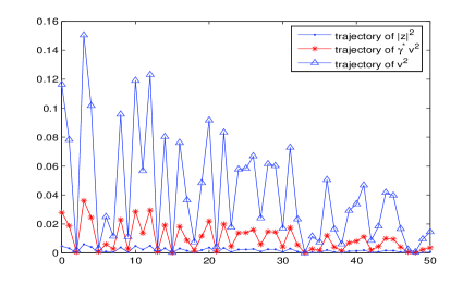
Figure 1: Trajectories of $|z|^{2},\gamma^{*^{2}}v^{2}$ and disturbance $v^{2}$ of system (64)

Example 5.2.

Considering the following stochastic system

$$\left\{\begin{array}[]{l}x^{(1)}_{k+1}=\theta^{(1)}_{k}x^{(1)}_{k}+\theta^{(2)}_{k}|x^{(2)}_{k}|^{2}+u^{(1)}_{k}+v^{(1)}_{k},\\ x^{(2)}_{k+1}=\theta^{(3)}_{k}x^{(2)}_{k}+\theta^{(4)}_{k}\frac{x^{(3)}_{k}}{1+|x^{(3)}_{k}|}+u^{(2)}_{k},\\ x^{(3)}_{k+1}=\theta^{(5)}_{k}x^{(3)}_{k}\cos(x^{(2)}_{k})+u^{(1)}_{k}+v^{(2)}_{k},\\ x^{(1)}_{0}\in\mathbb{R},x^{(2)}_{0}\in\mathbb{R},x^{(3)}_{0}\in(0,1),k\in\mathbb{N}\end{array}\right.$$ (70)

with the controlled output

$$z_{k}=\left[\begin{array}[]{c}0.1x^{(1)}_{k}+0.1x^{(3)}_{k}\cos(x^{(2)}_{k})\\ \frac{1}{7}|x^{(2)}_{k}|^{2}\\ u^{(1)}_{k}\end{array}\right],$$ (71)

where $\{\theta^{(i)}_{k},i=1,2,3,4,5\}_{k\in\mathbb{N}}$ are independently identically distributed random variable sequences, and $\theta^{(1)}_{k},\cdots,\theta^{(5)}_{k}$ are also independent of each other. Moreover, $\theta^{(1)}_{k}$, $\theta^{(3)}_{k}$, $\theta^{(4)}_{k}$ and $\theta^{(5)}_{k}$ are uniformly distributed on $[0,1]$, and $\theta^{(2)}_{k}$ is uniformly distributed on $[-1/2,1/2]$. $\{u^{(1)}_{k},u^{(2)}_{k}\}_{k\in\mathbb{N}}$ are the control sequences and $\{v^{(1)}_{k}\}_{k\in\mathbb{N}}$ is the exogenous disturbance sequence.

Denote $\omega_{k}=(\theta^{(1)}_{k},\theta^{(2)}_{k},\theta^{(3)}_{k},\theta^{(4)}_{k},\theta^{(5)}_{k})^{T}$, $x=(x^{(1)},x^{(2)},x^{(3)})^{T}$, $u=(u^{(1)},u^{(2)})^{T}$ and $v=(v^{(1)},v^{(2)})^{T}$, then the corresponding $f$, $g$, $m$ and $m_{1}$ in (11) can be written as

$$f(x,u,\omega_{k})=\left[\begin{array}[]{c}\theta^{(1)}_{k}x^{(1)}+\theta^{(2)}_{k}(x^{(2)})^{2}+u^{(1)}\\ \theta^{(3)}_{k}x^{(2)}+\theta^{(4)}_{k}\frac{x^{(3)}}{1+|x^{(3)}|}+u^{(2)}\\ \theta^{(5)}_{k}x^{(3)}\cos(x^{(2)})+u^{(1)}\end{array}\right],\ \ g(x,\omega_{k})=\left[\begin{array}[]{cc}1&0\\ 0&0\\ 0&1\end{array}\right],$$

$$m(x,u)=\left[\begin{array}[]{c}0.1x^{(1)}+0.1x^{(3)}\cos(x^{(2)})\\ \frac{1}{7}(x^{(2)})^{2}\\ u^{(1)}\end{array}\right],\ \ m_{1}(x)=0.$$

Suppose the function $V:\mathbb{R}^{3}\rightarrow\mathbb{R}^{+}$ has the form of

$$V(x)=p_{1}(x^{(1)})^{2}+p_{2}(x^{(2)})^{4}+p_{3}(x^{(3)})^{2}.$$ (72)

For each $\beta>1$, we have

$$\mathcal{H}(V(x),u,\beta) = \beta\mathbb{E}\bigg{[}p_{1}(\theta^{(1)}_{k}x^{(1)}+\theta^{(2)}_{k}(x^{(2)})^{2}+u^{(1)})^{2}+p_{2}(\theta^{(3)}_{k}x^{2}+\theta^{(4)}_{k}\frac{x^{(3)}}{1+|x^{(3)}|}+u^{(2)})^{4}$$

$$+p_{3}(\theta^{(5)}_{k}\cos(x^{(2)})x^{(3)}+u^{(1)})^{2}\bigg{]}-[p_{1}(x^{(1)})^{2}+p_{2}(x^{(2)})^{4}+p_{3}(x^{(3)})^{2}]$$

$$+0.01[x^{(1)}+x^{(3)}\cos(x^{(2)})]^{2}+\frac{1}{49}(x^{(2)})^{4}+(u^{(1)})^{2}$$

and

$$G_{\beta}(V(x))=\frac{\beta}{\beta-1}\sup\limits_{0\neq v\in\mathbb{R}^{2}}\frac{p_{1}(v^{(1)})^{2}+p_{3}(v^{(2)})^{2}}{|v|^{2}}=\frac{\beta}{\beta-1}\max(p_{1},p_{3}).$$

For $\gamma=0.75$, taking

$$\beta=\sqrt[3]{8/5},p_{1}=p_{2}=p_{3}=p=\frac{1}{16},$$

$$u^{(1)*}=-\frac{\beta^{3}p}{4\beta^{3}p+2}[x^{(1)}+x^{(3)}\cos(x^{(2)})]$$

and $u^{(2)*}=-\frac{1}{2}[x^{(2)}+\frac{x^{(3)}}{1+|x^{(3)}|}]$, we have

$$\mathcal{H}(V(x),u^{*},\beta) \leq p\beta^{3}\mathbb{E}\bigg{[}(\theta^{(1)}_{k}x^{(1)}+\theta^{(2)}_{k}(x^{(2)})^{2}+u^{(1)*})^{2}+(\theta^{(3)}_{k}x^{(2)}+\theta^{(4)}_{k}\frac{x^{(3)}}{1+|x^{(3)}|}+u^{(2)*})^{4}$$

$$+(\theta^{(5)}_{k}\cos(x^{(2)})x^{(3)}+u^{(1)*})^{2}\bigg{]}-p[(x^{(1)})^{2}+(x^{(2)})^{4}+(x^{(3)})^{2}]$$

$$+0.01[x^{(1)}+x^{(3)}\cos(x^{(2)})]^{2}+\frac{1}{49}(x^{(2)})^{4}+|u^{(1)*}|^{2}$$

$$= (2p\beta^{3}+1)\bigg{[}u^{(1)*}+\frac{p\beta^{3}}{2(2p\beta^{3}+1)}(x^{(1)}+x^{(3)}\cos(x^{(2)}))\bigg{]}^{2}$$

$$+p\beta^{3}\bigg{[}\theta^{(3)}_{k}x^{(2)}+\theta^{(4)}_{k}\frac{x^{(3)}}{1+|x^{(3)}|}+u^{(2)*}\bigg{]}^{4}$$

$$+p\beta^{3}\bigg{[}\frac{1}{3}(x^{(1)})^{2}+\frac{1}{12}(x^{(2)})^{4}+\frac{1}{3}|\cos(x^{(2)})|^{2}(x^{(3)})^{2}\bigg{]}$$

$$-\frac{p^{2}\beta^{6}}{4(2p\beta^{3}+1)}[x^{(1)}+x^{(3)}\cos(x^{(2)})]^{2}-p(x^{(1)})^{2}$$

$$-p(x^{(2)})^{4}-p(x^{(3)})^{2}+0.01[x^{(1)}+x^{(3)}\cos(x^{(2)})]^{2}+\frac{1}{49}(x^{(2)})^{4}$$

$$=p\beta^{3}\bigg{[}\frac{1}{80}(x^{(2)})^{4}+\frac{1}{24}\frac{(x^{(2)})^{2}(x^{(3)})^{2}}{(1+|x^{(3)}|)^{2}}$$

$$\quad+\frac{1}{80}\frac{(x^{(3)})^{4}}{(1+|x^{(3)}|)^{4}}+\frac{1}{3}(x^{(1)})^{2}+\frac{1}{12}(x^{(2)})^{4}$$

$$\quad+\frac{1}{3}|\cos(x^{(2)})|^{2}(x^{(3)})^{2}\bigg{]}-\frac{p^{2}\beta^{6}}{4(2p\beta^{3}+1)}[x^{(1)}+x^{(3)}\cos(x^{(2)})]^{2}$$

$$\quad-p(x^{(1)})^{2}-p(x^{(2)})^{4}-p(x^{(3)})^{2}+0.01[x^{(1)}+x^{(3)}\cos(x^{(2)})]^{2}+\frac{1}{49}(x^{(2)})^{4}$$

$$\leq p\beta^{3}\bigg{[}\frac{1}{80}(x^{(2)})^{4}+\frac{1}{24}\frac{(x^{(2)})^{2}(x^{(3)})^{2}}{(1+|x^{(3)}|)^{2}}+\frac{1}{80}\frac{(x^{(3)})^{4}}{(1+|x^{(3)}|)^{4}}$$

$$\quad+\frac{1}{3}(x^{(1)})^{2}+\frac{1}{12}(x^{(2)})^{4}+\frac{1}{3}|\cos(x^{(2)})|^{2}(x^{(3)})^{2}\bigg{]}$$

$$\quad-p(x^{(1)})^{2}-p(x^{(2)})^{4}-p(x^{(3)})^{2}+0.01[x^{(1)}+x^{(3)}\cos(x^{(2)})]^{2}+\frac{1}{49}(x^{(2)})^{4}$$

$$\leq p\beta^{3}\bigg{[}\frac{1}{80}(x^{(2)})^{4}+\frac{1}{24}\frac{(x^{(2)})^{2}(x^{(3)})^{2}}{(1+|x^{(3)}|)^{2}}+\frac{1}{80}\frac{(x^{(3)})^{4}}{(1+|x^{(3)}|)^{4}}$$

$$\quad+\frac{1}{3}(x^{(1)})^{2}+\frac{1}{12}(x^{(2)})^{4}+\frac{1}{3}(x^{(3)})^{2}\bigg{]}$$

$$\quad-p(x^{(1)})^{2}-p(x^{(2)})^{4}-p(x^{(3)})^{2}+0.02[(x^{(1)})^{2}+(x^{(3)})^{2}]+\frac{1}{49}(x^{(2)})^{4}$$

$$\leq p\beta^{3}\bigg{[}\frac{1}{80}(x^{(2)})^{4}+\frac{1}{48}((x^{(2)})^{4}+(x^{(3)})^{2})+\frac{1}{80}(x^{(3)})^{2}$$

$$\quad+\frac{1}{3}(x^{(1)})^{2}+\frac{1}{12}(x^{(2)})^{4}+\frac{1}{3}(x^{(3)})^{2}\bigg{]}$$

$$\quad-p(x^{(1)})^{2}-p(x^{(2)})^{4}-p(x^{(3)})^{2}+0.02[(x^{(1)})^{2}+(x^{(3)})^{2}]+\frac{1}{49}(x^{(2)})^{4}$$

$$=[\frac{p\beta^{3}}{3}+0.02-p](x^{(1)})^{2}+[p\beta^{3}(\frac{1}{12}+\frac{1}{80}+\frac{1}{48})+\frac{1}{49}-p](x^{(2)})^{4}$$

$$\quad+[p\beta^{3}(\frac{1}{3}+\frac{1}{48}+\frac{1}{80})+0.02-p](x^{(3)})^{2}$$

$$\leq\left[\frac{5}{12}p\beta^{3}+\frac{1}{48}-p\right]\left[(x^{(1)})^{2}+(x^{(2)})^{4}+(x^{(3)})^{2}\right]$$

$$=0.$$

As far as

$$G_{\beta}(V(x))=\frac{\beta}{\beta-1}\frac{1}{16}\leq\gamma^{2},$$

it can be obtained by the fact that

$$5\times 8^{3}\beta^{3}=8^{4}=4096>3645=5\times 9^{3}.$$

So, for any $x\in\mathbb{R}^{3}$, the above given $V(x)$, $u^{*}=(u^{(1)*},u^{(2)*})^{T}$ and $\beta$ satisfy conditions of (58) and (59). According to Theorem 4.2, $u^{*}=(u^{(1)*},u^{(2)*})^{T}$ is the corresponding $H_{\infty}$ control of system (70). Moreover, system (70) is internally stable under the $H_{\infty}$ control $u^{*}$. Fig.2 shows the trajectories of $H_{\infty}$ control $u^{(1)*}$ and $u^{(2)*}$. Fig.3 shows the samples of the trajectories of the states $x^{(1)}$, $x^{(2)}$ and $x^{(3)}$ under the control $u^{*}$. Fig.4 shows the trajectories of $\gamma^{2}|v|^{2}$ and $|z|^{2}$. From Fig.4, we see that $\|\mathcal{L}_{u^{*}}\|\leq\gamma$, which verifies the correctness of Theorem 4.2.

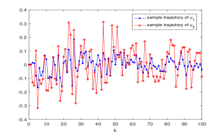
Figure 2: Trajectories of $H_{\infty}$ control $u^{*}$ for system (70)

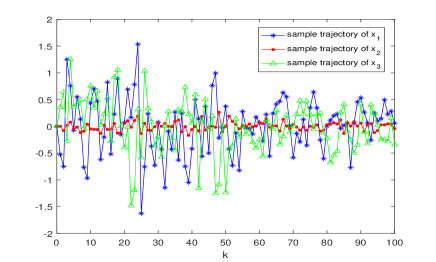
Figure 3: Trajectories of system (70) under $H_{\infty}$ control

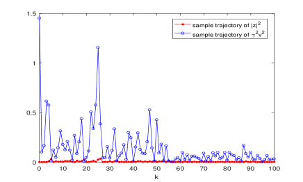
Figure 4: Trajectories of $|z|^{2}$ and $\gamma^{2}v^{(2)}$ of system (70) under $H_{\infty}$ control

6 Conclusions

We have introduced the convex analysis method to study the $H_{\infty}$ control for more general discrete-time nonlinear stochastic systems (see systems (11) and (53)), based on which, a stochastic version of bounded real lemma for discrete-time nonlinear stochastic systems has been obtained. It can be found that our concerned systems are more general than affine nonlinear system (1). It is expected that the developed convex analysis technique can also be applied to deal with the output feedback $H_{\infty}$ control and other robust control problems such as in [36].

References

• [1] G. Zames, “Feedback and optimal sensitivity: Model reference transformations, multiplicative seminorms, and approximate inverses,” IEEE Trans. Autom. Control, 26 (2), pp. 301-320, 1981.
• [2] T. Basar and P. Bernhard, $H^{\infty}$-Optimal Control and Related Minimax Design Problems–A Dynamic Game Approach. Birkhäuser, Boston, 1995.
• [3] B. A. Francis and J. C. Doyle, “Linear control theory with an $H_{\infty}$ optimality criterion,” SIAM J. Control and Optimization, 25(4), pp. 815–844, 1987.
• [4] J. C. Doyle, K. Glover, P. Khargonekar, and B. Francis, “State-space solutions to standard $H_{2}$ and $H_{\infty}$ control problems,” IEEE Trans. Autom. Control, 34, pp. 831–847, 1989.
• [5] K. Zhou and J. C. Doyle, Essentials of Robust Control, Prentice Hall Inc., 1998.
• [6] Z.P. Hu and F. Q. Deng, “Robust $H_{\infty}$ control for networked systems with transmission delays and successive packet dropouts under stochastic sampling,” Int. J. Robust Nonlinear Control, 27, pp. 84–107, 2017.
• [7] C. H. Wu, W. Zhang, and B. S. Chen, “Multiobjective $H_{2}/H_{\infty}$ synthetic gene network design based on promoter libraries,” Mathematical Biosciences, 233(2), 111-125, 2011.
• [8] B. S. Chen, C. H. Chang, and H.C. Lee, “Robust synthetic biology design: stochastic game theory approach,” Bioinformatics, 25(14), pp. 1822–1830, 2009.
• [9] P. Gahinet and P. Apkarian, “A linear matrix inequality approach to $H^{\infty}$ control,” Int. J. Robust Nonlinear Control, 4, pp. 421–448, 1994.
• [10] A. J. Van der Schaft, “On a state-space appoach to nonlinear $H_{\infty}$ control,” Systems & Control Letters, 16, pp. 1–8, 1991.
• [11] J. A. Ball, J. W. Helton, and M. L. Walker, “$H_{\infty}$ control for nonlinear systems with output feedback,” IEEE Trans. Autom. Control, 38(4), pp.546–559, 1993.
• [12] A. Isidori and A. Astolfi, “Disturbance attenuation and $H_{\infty}$-control via measurement feedback in nonlinear systems,” IEEE Trans. Autom. Control, 37, pp.1283–1293, 1992.
• [13] D. Hinrichsen and A.J. Pritchard, “Stochastic $H^{\infty}$,” SIAM J. Control and Optimization, 36(5), pp. 1504–1538, 1998.
• [14] V. A. Ugrinovskii. Robust $H^{\infty}$ control in the presence of stochastic uncertainty. Int. J. Control, 71: 219-237, 1998.
• [15] I. R. Petersen, V. A. Ugrinovskii, and A. V. Savkin, Robust Control Design Using $H_{\infty}$ Methods. New York: Springer-Verlag, 2000.
• [16] A. Germani, C. Manes, and P. Palumbo, “Filtering of stochastic nonlinear differential systems via a Carleman approximation,” IEEE Trans. Autom. Control, 52(11), pp. 2166-2172, 2007.
• [17] W. Zhang and B. S. Chen, “State feedback $H_{\infty}$ control for a class of nonlinear stochastic systems,” SIAM J. Control and Optimization, 44(6), pp. 1973–1991, 2006.
• [18] W. Zhang, B. S. Chen, and C. S. Tseng, “Robust $H_{\infty}$ filtering for nonlinear stochastic systems,” IEEE Trans. Signal Process., 53, pp. 589–598, 2005.
• [19] W. Zhang, L. Xie, and B. S. Chen. Stochastic $H_{2}/H_{\infty}$ Control: A Nash Game Approach, Taylor $\&$ Francis, 2017.
• [20] E. K. Boukas, Z. K. Liu and G. X. Liu, “Delay-dependent robust stability and $H_{\infty}$ control of jump linear systems,” Int. J. Control, 74(4), pp. 329–340, 2001.
• [21] S. Xu, J. Lam, and X. Mao, “Delay-dependent $H_{\infty}$ control and filtering for uncertain Markovian jump systems with time-varying delays,” IEEE Trans. Circuits Systems, 54(9), pp. 2070–2077, 2007.
• [22] V. Dragan, T. Morozan, and A. M. Stoica. Mathematical Methods in Robust Control of Linear Stochastic Systems. New York: Springer, 2006.
• [23] X. Lin and R. Zhang, “$H_{\infty}$ control for stochastic systems with Poisson jumps,” J. Syst. Sci. Complex., 24(4), pp. 683–700, 2011.
• [24] B. S. Chen and C.F. Wu, “Robust scheduling filter design for a class of nonlinear stochastic Poisson signal systems,” IEEE Trans. Signal Process., 63(23), pp. 6245–6257, 2015.
• [25] W. Lin and C. I. Byrnes, “$H_{\infty}$-control of discrete-time nonlinear systems,” IEEE Trans. Autom. Control, 41(4), pp.494–510, 1996.
• [26] A. El Bouhtouri, D. Hinrichsen and A. J. Pritchard, $H_{\infty}$ Type Control for Discrete-Time Stochastic Systems, International Journal of Robust and Nonlinear Control, 9(13), pp.923–948, 1999.
• [27] W. Zhang, Y. Huang, and L. Xie, Infinite horizon stochastic $H_{2}/H_{\infty}$ control for discrete-time systems with state and disturbance dependent noise, Automatica, 44, pp. 2306–2316, 2008.
• [28] V. Dragan, T. Morozan, and A. M. Stoica. Mathematical Methods in Robust Control of Discrete-Time Linear Stochastic Systems. New York: Springer, 2010.
• [29] N. Berman and U. Shaked, “$H_{\infty}$ control for discrete-time nonlinear stochastic systems.,” IEEE Trans. Autom. Control, 51(6), pp. 1041–1046, 2006.
• [30] X. Lu and W. Zhang, “Stochastic finite horizon $H_{\infty}$ control for nonlinear discrete-time systems,” Proceedings of the 27th Chinese Control Conference, July 16-18, 2008, Kunming, Yunnan Province, China , pp. 789-793, 2008.
• [31] B. Shen, Z. Wang, H. Shu, and G. Wei, “$H_{\infty}$ filtering for nonlinear discrete-time stochastic systems with randomly varying sensor delays,” Automatica, 45, pp. 1032–1037, 2009.
• [32] H. Li and Y. Shi, “Robust $H_{\infty}$ filtering for nonlinear stochastic systems with uncertainties and Markov delays,” Automatica, 48, pp. 159-166, 2012.
• [33] O. Kallenberg, Foundations of Mordern Probability, New York: Springer-Verlag, 2002.
• [34] W. Zhang, X. Lin, and B.S. Chen, “LaSalle-type theorem and its applications to infinite horizon optimal control of discrete-time nonlinear stochastic systems,” IEEE Trans. Autom. Control, 62(1), pp.250–261, 2017.
• [35] P. Montel, Sur les fonctions convexes et les fonctions sousharmoniques, J. Math. Pures Appl., 7(9), pp.29–60, 1928.
• [36] W. Lin and C. I. Byrnes, “Discrete-time nonlinear $H_{\infty}$ control with measurement feedback,” Aumnatica, 31(3), pp. 419-434, 1995.