Electromagnetic reactions from coupled-cluster theory

Abstract

We review recent results for electromagnetic reactions and related sum rules in light and medium-mass nuclei obtained from coupled-cluster theory. In particular, we highlight our recent computations of the photodisintegration cross section of ⁴⁰Ca and of the electric dipole polarizability for oxygen and calcium isotopes. We also provide new results for the Coulomb sum rule for ⁴He and ¹⁶O. For ⁴He we perform a thorough comparison of coupled-cluster theory with exact hyperspherical harmonics.

1 Introduction

Electromagnetic reactions have traditionally been a golden tool for studying nuclear dynamics. They lead, for instance, to the discovery of giant dipole resonances and their interpretation in terms of collective modes [1, 2]. While a complete body of data has been collected over the years for stable nuclei, only recently have we begun to elucidate them in terms of first principle calculations. This was achieved thanks to the introduction of a new ab initio computational tool, obtained from a coupled cluster theory formulation of the Lorentz integral transform method [3], which we will review below.

The key ingredient to study reactions induced by external electromagnetic probes, such as photons or electrons, is the nuclear response function. The latter is defined as

$$R(\omega,q)=\sum_{f}\left|\langle\psi_{f}|\hat{\Theta}(q)|\psi_{0}\rangle\right|^{2}\delta\left(E_{f}-E_{0}-\omega\right),$$ (1)

where $\hat{\Theta}(q)$ is the excitation operator, which will in general depend on the momentum-transfer $q$ and whose form will be specific to the considered probe. The nuclear response function is a dynamical observables which requires knowledge on the whole spectrum of the nucleus, being $|\psi_{0}\rangle$ and $|\psi_{f}\rangle$ the ground- and excited-states, respectively. The difficulty of studying Eq. (1) lies in the fact that one needs, in principle, to calculate all the excited states $|\psi_{f}\rangle$, including all open channels in the continuum. While this is possible for two- and three-body problems, starting at four nucleons it can only be done with restrictions in energy and/or with approximations. To overcome this complication, one can employ the Lorentz integral transform (LIT) [4] and reduce the problem to the solution of a bound state equation. In this approach, rather than directly calculating $R(\omega,q)$, one computes the following transform

$${L}(q,\omega_{0},\Gamma)=\int_{\omega_{\rm th}}^{\infty}d\omega\frac{R(\omega,q)}{(\omega-\omega_{0})^{2}+\Gamma^{2}}\>\mbox{.}$$ (2)

Here $\omega_{\rm th}$ is the threshold energy and $\Gamma>0$ is the Lorentzian width, which plays the role of a resolution parameter. By using the closure relation one finds

$${L}(q,z)=\langle\psi_{0}|{\hat{\Theta}}^{\dagger}(q)\frac{1}{\hat{H}-z^{*}}\frac{1}{\hat{H}-z}\hat{\Theta}(q)|\psi_{0}\rangle=\langle\widetilde{\psi}|\widetilde{\psi}\rangle\>\mbox{,}$$ (3)

where we introduced the complex energy $z=E_{0}+\omega_{0}+i\Gamma$ and $\hat{H}$ is the nuclear Hamiltonian, which will be taken from chiral effective field theory [5, 6]. The LIT of the response function, ${L}(q,z)$, can be computed directly by solving the Schrödinger-like equation

$$(\hat{H}-z)|\widetilde{\psi}\rangle=\hat{\Theta}(q)|\psi_{0}\rangle\>\hskip 28.45274pt$$ (4)

for different values of $z$. The solution $|\widetilde{\psi}\rangle$ has bound-state-like asymptotic, thus $L(q,z)$ can be calculated even for $A>3$ with any good bound-state method, such as hyperspherical harmonics expansions [7]. Results for $R(q,\omega)$ are obtained from an inversion of the LIT and are independent on the choice of $\Gamma$ [4].

Recently, we have merged the advantage of the LIT method with the mild computational scaling that characterizes coupled-cluster theory [8] for increasing mass number, obtaining a new computational tool [3]. In coupled-cluster theory, as originally introduced by Coester and Kümmel [9], the exact many-body wave function is written in the exponential ansatz

$$|\Psi_{0}\rangle=\exp{(T)}|{\rm\Phi_{0}}\rangle\,,$$ (5)

where $|{\rm\Phi_{0}}\rangle$ is a Slater determinant. The operator $T$, typically expanded in $n$-particle-$n$-hole excitations (or clusters) $T=T_{1}+T_{2}+\dots+T_{A}$, is responsible for introducing correlations.

The LIT method in the coupled-cluster language requires the solution of a bound-state equation

$$(\overline{H}-z)|{\tilde{\Psi}}_{R}(z)\rangle=\overline{\Theta}(q)|0_{R}\rangle\;,$$ (6)

where the right ground-state $|0_{R}\rangle\equiv|\Phi_{0}\rangle$, while $\overline{H}$ and $\overline{\Theta}$ are the similarity transformed Hamiltonian and excitation operators, respectively

$$\overline{H} = \exp(-T)\hat{H}\exp(T)\,,$$ (7)

$$\overline{\Theta} = \exp(-T)\hat{\Theta}\exp(T)\,.$$ (8)

The solution of Eq. (6) is found as linear superposition of particle-hole excitation on top of the reference Slater determinant as

$$|\widetilde{\Psi}_{R}(z)\rangle = {\cal R}(z)|\Phi_{0}\rangle=({\mathcal{R}}_{1}+{\mathcal{R}}_{2}+\dots+{\mathcal{R}}_{A})|\Phi_{0}\rangle\;.$$

In Ref. [3] we have adopted the most commonly used approximation, i.e., the single and doubles scheme (CCSD), where $T=T_{1}+T_{2}$ and ${\mathcal{R}}={\mathcal{R}}_{1}+{\mathcal{R}}_{2}$ and have successfully benchmarked this method with exact hyperspherical harmonics on ⁴He, showing that the CCSD approximation differs only by 1-2$\%$ from the exact result.

Because the computational cost of the coupled-cluster method scales mildly with respect to the mass number, this theory paves the way for many future investigations of electroweak reactions in medium-mass nuclei, as it provides an ab initio approach where the continuum is properly taken into account.

2 The photodisintegration cross section

The first observables where we used the power of coupled-cluster theory to address medium-mass nuclei has been the photodisintegration cross section. In the unretarded dipole approximation, the photodisintegration cross section is

$$\sigma_{\gamma}(\omega)=4\pi^{2}\alpha\omega R(\omega)\,,$$ (9)

where $R(\omega)$ is the dipole response function, with $\omega=q$ for real photons. The excitation operator is the translationally invariant dipole operator

$$\hat{\Theta}=\sum_{k}^{A}\left({\bf r}_{k}-{\bf R}_{\rm cm}\right)\left(\frac{1+\tau^{3}_{k}}{2}\right)\,,$$ (10)

where ${\bf r}_{k}$ and ${\bf R}_{\rm cm}$ are the coordinates of the $k$-th particle and the center-of-mass, respectively, while $(1+\tau^{3}_{k})/2$ defines the projection operator on the $Z$ protons.

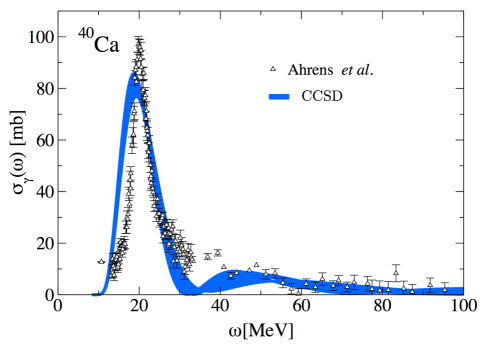
Figure 1: ⁴⁰Ca photodisintegration cross section at the CCSD level [10] compared to experimental data by Ahrens et al. [12]. Result are obtained with a two-nucleon chiral force [11]. Figure adapted from Ref. [10].

By solving Eq. (6) with the dipole operator in Eq. (10) we have been able, e.g., to calculate the photodisintegration cross section of ⁴⁰Ca [10] using a realistic two-body chiral potential [11]. Results are shown in Fig. 1. The width of the blue curve is obtained from various inversions of the integral transform and constitutes a lower band of the total theoretical error-bar associated to this observable. A very good description of this quantity with respect to the experimental data from Ref. [12] is obtained already at this level of approximation in coupled-cluster theory. This result highlights the relevance of the newly introduced method, which allowed $(i)$ to depart from the classical few-body systems and reach medium mass nuclei with only little more computational expense and $(ii)$ to obtain, for the first time, a microscopic description of experimental data in this mass range.

3 The electric dipole polarizability

We now focus our attention on the electric dipole polarizability. The latter is defined as an inverse energy weighted sum rule of the dipole response function

$$\alpha_{D}=2\alpha\int_{\omega_{ex}}^{\infty}d\omega~{}\frac{R(\omega)}{\omega}\,.$$ (11)

It is well known from the nuclear droplet and hydrodynamic models [13], as well as from density functional theory [14], that the electric dipole polarizability is correlated with the nuclear charge radius $r_{ch}$. Thus, it is interesting to see if this correlation is also observed in first principle calculations and the developed LIT-CC technology allows for such a study.

In order to study correlations, one needs a considerable number of interactions, such that results span a wide range of values both for the polarizability and the charge radius. For this purpose, we take some of the few realistic nucleon-nucleon interaction and evolve them with similarity transformations.

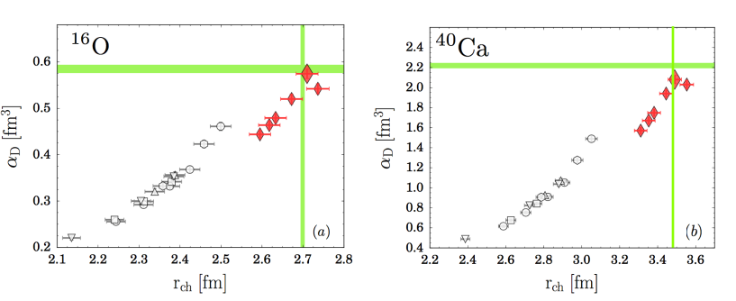
Figure 2: $\alpha_{D}$ versus $r_{ch}$ in ¹⁶O (a) and ⁴⁰Ca (b). Empty symbols refer to calculations with nucleon-nucleon potentials only. The red (full) diamonds refer to calculations that include three-body forces. Details on the potentials used are found in Ref. [15]. The green bands denote the experimental values for these two quantities. Figure adapted from Ref. [15].

Fig. 2 shows the correlation of the electric dipole polarizability $\alpha_{D}$ with the charge radius in ¹⁶O (a) and in ⁴⁰Ca (b). The empty symbols refer to calculations with two-body forces only. They clearly show a strong correlation between the two observables. On the other hand, one also observes that the use of two-body interactions only leads to a strong underestimation of the experimental values of both quantities, denoted by the green bands. When we include three-nucleon forces, by using a variety of Hamiltonians from chiral effective field theory [16, 17], we obtain the solid diamonds, which still exhibiting a strong correlation but cluster much closer to the experimental value. This fact indicates that three nucleon forces are important to obtain a correct description of both observables. It needs to be noted though, that we have made a specific choice of Hamiltonians, preferring those that provide a reasonable description of the charge radius. It is well known that other Hamiltonians from chiral effective field theory suffer from and under-estimation of the radii, which, in the light of Fig. 2, would also lead to an underestimation of the electric dipole polarizability. In particular, the largest diamond data are obtained with the NNLO_sat [17] potential, which has been fit to reproduce also the ¹⁶O charge radius. It is interesting to note that this constraint enables a correct prediction also for ⁴⁰Ca.

By studying similar correlations in ⁴⁸Ca and combining them with experimental information from electron scattering, we also were able to provide narrow constraints on the neutron skin thickness and on the electric dipole polarizability [18, 19].

4 The Coulomb sum rule

Finally, we turn our attention to the Coulomb sum rule. With the objective in mind to eventually tackle neutrino-nucleus interactions relevant for long-baseline neutrino experiments, we initiated a study of electron-scattering reactions within coupled-cluster theory. Following the work done with the Green’s function Monte Carlo method in Ref. [20], we first investigate the Coulomb sum rule.

Omitting for simplicity the role of the nucleon form factor, the longitudinal Coulomb sum rule is defined as as total strength of the inelastic longitudinal response function as

$$CSR(q)=\int_{\omega^{+}_{th}}^{\infty}d\omega R_{L}(\omega,q)\,,$$ (12)

where

$$R_{L}(\omega,q)=\int\!\!\!\!\!\!\!\sum_{f\neq 0}|\left\langle\Psi_{f}|\hat{\rho}(q)|\Psi_{0}\right\rangle|^{2}\delta\left(E_{f}+\frac{q^{2}}{2M}-E_{0}-\omega\right),\,$$ (13)

with $\hat{\rho}(q)$ being the charge operator and $\frac{\mathbf{q}^{2}}{2M}$ a recoil term. One possible approach to compute the Coulomb sum rule is to perform a multipole expansion of the charge operator and then solve Eq. (4) for every multipole on a grid of $q$, as was done in Ref. [21]. However, the Coulomb sum rule can be rewritten also as expectation value on the ground state which is much easier to calculate

$$CSR(q)=Z+\langle\psi_{0}|\sum_{i\neq j}e^{i{\bf q}\cdot{({\bf r}_{i}-{\bf r}_{j})}}|\psi_{0}\rangle-|F_{el}(q)|^{2}Z^{2}=Z+Z(Z-1)f_{2}(q)-|F_{el}(q)|^{2}Z^{2}\,,$$ (14)

where $f_{2}(q)$ is the Fourier transform of the proton-proton correlation density and $F_{el}(q)$ is the elastic form factor [22].

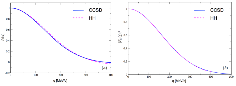
Figure 3: Comparison of CCSD and exact hyperspherical harmonics (HH) computations of $f_{2}(q)2$, panel (a) and $|F_{el}(q)|^{2}$, panel (b) as a function of the momentum transfer $q$ using a chiral two-body force [11].

To first compare the CCSD approximation with exact calculation we compare computations of $f_{2}(q)$ and $|F_{el}(q)|^{2}$ with exact hyperspherical harmonics, as shown in Fig. 3 vs. the momentum transfer. Calculations are performed with a chiral two-body force [11] and show a very nice agreement between the two methods, proving the CCSD approximation to be very reliable.

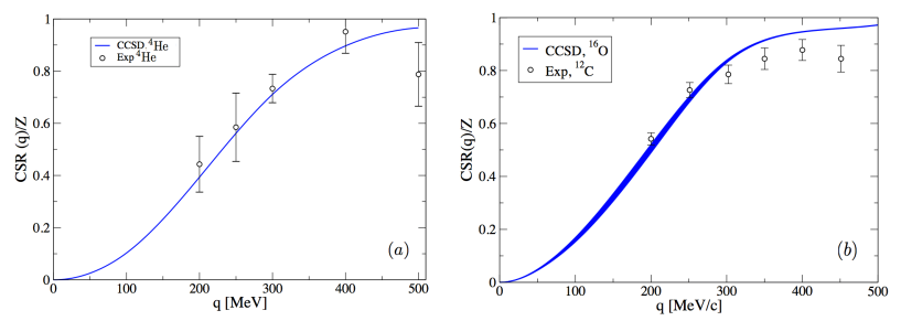
Figure 4: Coulomb sum rule for ⁴He (a) and ¹⁶O (b) from coupled-cluster theory using a chiral two-body force [11], compared to experimental results from [23, 24] for ⁴He (a), and from Ref. [25] for ¹²C (b).

In Fig. 4 we finally compare the Coulomb sum rule calculated from coupled-cluster theory for ⁴He and ¹⁶O with experimental data. Measurements of the longitudinal response functions at low momentum transfers ($q=200$ and $250$ MeV/c) are taken from Buki et al. [23], while intermediate momentum transfer values are collected in Ref. [24]. Unfortunately, no data exist for ¹⁶O, so we show data for ¹²C taken from [25]. Similar results were also obtained in Refs. [25, 26]. Fig. 4 shows that our calculations agree quite well with the experimental data. Thus, extensions to heavier nuclei and to neutrino reactions are promising.

5 Conclusions

We reviewed some of our recent results on electromagnetic reactions and related sum rules obtained from coupled cluster theory and the Lorentz integral transform. The method has allowed us to surpass previous mass limits and paves the way for ab initio studies of neutrino-nucleus cross section. We addressed first electron scattering observables, such as the Coulomb sum rule, and performed a comparison to exact calculations and to data. This is essential for any theory that is going to be used to model neutrino-nucleus interactions.

5.1 Acknowledgments

This work was supported in parts by the Natural Sciences and Engineering Research Council (NSERC), the National Research Council of Canada, the PRISMA Cluster of Excellence and the Sonderforschungbereich CRC 1044.

References

References

- [1] Goldhaber M and Teller E 1948 Phys. Rev. 74 1046
- [2] Steinwedel H and Jensen J H D 1950 Z. Naturforsch 5A 413
- [3] Bacca S et al. 2013 Phys. Rev. Lett. 111 122502
- [4] Efros V D et al 2007 Journal of Physics G: Nuclear and Particle Physics 34 R459
- [5] Epelbaum E, Hammer H-W and Meißner U-G 2009 Rev. Mod. Phys. 81 1773
- [6] Machleidt R and Entem D R 2011 Physics Reports 503 1
- [7] Barnea N, Leidemann W and Orlandini G 2001 Nuclear Physics A 693 565
- [8] Hagen G, Papenbrock T, Hjorth-Jensen M and Dean D J 2014 Rep. Prog. Phys. 77 096302
- [9] Coester F and Kümmel H 1960 Nucl. Phys. 17 477
- [10] Bacca S, Barnea N, Hagen G, Miorelli M, Orlandini G and Papenbrock T 2014 Phys. Rev. C 90 064619
- [11] Entem D R and Machleidt R 2003 Phys. Rev. C 68 041001
- [12] Ahrens J et al. 1975 Nucl. Phys. A 251, 479
- [13] Lipparini E and Stringari S 1989 Phys. Rep. 175 104
- [14] Roca-Maza X et al. 2015 Phys. Rev. C 82 064304
- [15] Miorelli M, Bacca S, Barnea N, Hagen G, Jansen G R, Orlandini G, Papenbrock T 2016 Phys. Rev. C 94 034317
- [16] Hebeler K and Bogner S K, Furnstahl R J, Nogga A and Schwenk A 2011 Phys. Rev. C 83, 031301
- [17] Ekström A et al. 2015 Phys. Rev. C, 91 051301
- [18] Hagen G et al. 2016 Nature Physics 12, 186
- [19] Birkhan J et al. 2017 Phys. Rev. Lett. 118 252501
- [20] A. Lovato et al. 2013 Phys. Rev. Lett. 111 092501
- [21] Bacca S, Barnea N, Leidemann W and Orlandini G 2009 Phys. Rev. C 80 064001
- [22] Orlandini G and Traini M 1991 Rep. Prog. Phys. 54 257
- [23] Buki A et al. 2006 Phys. Lett. B 641, 156
- [24] Carlson J, Jourdan J, Schiavilla R and Sick I 2002 Phys. Rev. C 65, 024002
- [25] Mihaila B and Heisenberg H J 2000 Phys. Rev. Lett. 84 1403
- [26] Lonardoni D et al. 2017 Phys. Rev. C 96 024326