Estimating long memory in panel random-coefficient AR(1) data

Abstract

We construct an asymptotically normal estimator $\widetilde{\beta}_{N}$ for the tail index $\beta$ of a distribution on $(0,1)$ regularly varying at $x=1$, when its $N$ independent realizations are not directly observable. The estimator $\widetilde{\beta}_{N}$ is a version of the tail index estimator of Goldie and Smith (1987) based on suitably truncated observations contaminated with arbitrarily dependent ‘noise’ which vanishes as $N$ increases. We apply $\widetilde{\beta}_{N}$ to panel data comprising $N$ random-coefficient AR(1) series, each of length $T$, for estimation of the tail index of the random coefficient at the unit root, in which case the unobservable random coefficients are replaced by sample lag 1 autocorrelations of individual time series. Using asymptotic normality of $\widetilde{\beta}_{N}$, we construct a statistical procedure to test if the panel random-coefficient AR(1) data exhibit long memory. A simulation study illustrates finite-sample performance of the introduced inference procedures.

Keywords: random-coefficient autoregression; tail index estimator; measurement error; panel data; long memory process.

2010 MSC: 62G32, 62M10.

1 Introduction

Dynamic panels (or longitudinal data) comprising observations taken at regular time intervals for the same individuals such as households, firms, etc. in a large heterogeneous population, are often described by time series models with random parameters (for reviews on dynamic panel data analysis, see Arellano  (2003), Baltagi  (2015)). One of the simplest models for individual evolution is the random-coefficient AR(1) (RCAR(1)) process

$$X_{i}(t)=a_{i}X_{i}(t-1)+\zeta_{i}(t),\quad t\in\mathbb{Z},\quad i=1,2,\dots,$$ (1)

where the innovations $\zeta_{i}(t)$, $t\in\mathbb{Z}$, are independent identically distributed (i.i.d.) random variables (r.v.s) with $\mathbb{E}\zeta_{i}(t)=0$, $\mathbb{E}\zeta^{2}_{i}(t)<\infty$ and the autoregressive coefficient $a_{i}\in(0,1)$ is a r.v., independent of $\{\zeta_{i}(t),\,t\in\mathbb{Z}\}$. It is assumed that the random coefficients $a_{i}$, $i=1,2,\dots$, are i.i.d., while the innovation sequences $\{\zeta_{i}(t),t\in\mathbb{Z}\}$ can be either independent or dependent across $i$, by inclusion of a common ‘shock’ to each unit; see Assumptions (A1)–(A4) below. If the distribution of $a_{i}$ is sufficiently ‘dense’ near unity, then statistical properties of the individual evolution in (1) and the corresponding panel can differ greatly from those in the case of fixed $a\in(0,1)$. To be more specific, assume that the AR coefficient $a_{i}$ has a density function $g(x)$, $x\in(0,1)$, satisfying

$$g(x)\sim g_{1}(1-x)^{\beta-1},\quad x\to 1-,$$ (2)

for some $\beta>1$ and $g_{1}>0$. Then a stationary solution of RCAR(1) equation (1) has the following autocovariance function

$$\mathbb{E}X_{i}(0)X_{i}(t)=\mathbb{E}\zeta^{2}_{i}(0)\mathbb{E}\frac{a^{|t|}_{i}}{1-a^{2}_{i}}\sim\frac{g_{1}}{2}\Gamma(\beta-1)\mathbb{E}\zeta^{2}_{i}(0)t^{-(\beta-1)},\quad t\to\infty,$$ (3)

and exhibits long memory in the sense that $\sum_{t\in\mathbb{Z}}|\operatorname{Cov}(X_{i}(0),X_{i}(t))|=\infty$ for $\beta\in(1,2]$. The same long memory property applies to the contemporaneous aggregate

$$\bar{X}_{N}(t):=N^{-1/2}\sum_{i=1}^{N}X_{i}(t),\quad t\in\mathbb{Z},$$ (4)

of $N$ independent individual evolutions in (1) and its Gaussian limit arising as $N\to\infty$. For the beta distributed squared AR coefficient $a_{i}^{2}$, these facts were first uncovered by Granger  (1980) and later extended to more general distributions and/or RCAR equations in Gonçalves and Gouriéroux  (1988), Zaffaroni  (2004), Celov et al.  (2007), Oppenheim and Viano  (2004), Puplinskaitė and Surgailis  (2010), Philippe et al.  (2014) and other works, see Leipus et al.  (2014) for review. Assumption (2) and the parameter $\beta$ play a crucial role for statistical (dependence) properties of the panel $\{X_{i}(t),\,t=1,\dots,T,\,i=1,\dots,N\}$ as $N$ and $T$ increase, possibly at different rates. Particularly, Pilipauskaitė and Surgailis  (2014) proved that for $\beta\in(1,2)$ the distribution of the normalized sample mean $\sum_{i=1}^{N}\sum_{t=1}^{T}X_{i}(t)$ is asymptotically normal if $N/T^{\beta}\to\infty$ and $\beta$-stable if $N/T^{\beta}\to 0$ (in the ‘intermediate’ case $N/T^{\beta}\to c\in(0,\infty)$ this limit distribution is more complicated and given by an integral with respect to a certain Poisson random measure). In the case of common innovations ($\{\zeta_{i}(t),\ t\in\mathbb{Z}\}\equiv\{\zeta(t),\ t\in\mathbb{Z}\}$) the limit stationary aggregated process exists under a different normalization ($N^{-1}$ instead of $N^{-1/2}$ in (4)) and is written as a moving-average in the above innovations with deterministic coefficients $\mathbb{E}a_{1}^{j}$, $j\geq 0$, which decay as $\Gamma(\beta)j^{-\beta}$ with $j\to\infty$ and exhibit long memory for $\beta\in(1/2,1)$; see Zaffaroni  (2004), Puplinskaitė and Surgailis  (2009). The trichotomy of the limit distribution of the sample mean for a panel comprising RCAR(1) series driven by common innovations is discussed in Pilipauskaitė and Surgailis  (2015).

In the above context, a natural statistical problem concerns inference about the distribution of the random AR coefficient $a_{i}$, e.g., its cumulative distribution function (c.d.f.) $G$ or the parameter $\beta$ in (2). Leipus et al.  (2006), Celov et al.  (2010) estimated the density $g$ using sample autocovariances of the limit aggregated process. For estimating parameters of $G$, Robinson  (1978) used the method of moments. He proved asymptotic normality of the estimators for moments of $G$ based on the panel RCAR(1) data as $N\to\infty$ for fixed $T$, under the condition $\mathbb{E}(1-a^{2}_{i})^{-2}<\infty$ which does not allow for long memory in $\{X_{i}(t),\,t\in\mathbb{Z}\}$. For parameters of the beta distribution, Beran et al.  (2010) discussed maximum likelihood estimation based on (truncated) sample lag 1 autocorrelations computed from $\{X_{i}(1),\dots,X_{i}(T)\}$, $i=1,\dots,N$, and proved consistency and asymptotic normality of the introduced estimator as $N,T\to\infty$. In nonparametric context, Leipus et al.  (2016) studied the empirical c.d.f. of $a_{i}$ based on sample lag 1 autocorrelations similarly to Beran et al.  (2010), and derived its asymptotic properties as $N,T\to\infty$, including those of a kernel density estimator. Moreover, Leipus et al.  (2016) proposed another estimator of moments of $G$ and proved its asymptotic normality as $N,T\to\infty$. Except for parametric situations, the afore mentioned results do not allow for inferences about the tail parameter $\beta$ in (2) and testing for the presence or absence of long memory in panel RCAR(1) data.

The present paper discusses in semiparametric context, the estimation of $\beta$ in (2) from RCAR(1) panel $\{X_{i}(t),\,t=1,\dots,T,\,i=1,\dots,N\}$ with finite variance $\mathbb{E}X_{i}^{2}(t)<\infty$. We use the fact that (2) implies $\mathbb{P}(1/(1-a_{i})>y)\sim(g_{1}/\beta)y^{-\beta}$, $y\to\infty$, i.e. r.v. $1/(1-a_{i})$ follow a heavy-tailed distribution with index $\beta>1$. Thus, if $a_{i}$, $i=1,\dots,N$, were observed, $\beta$ could be estimated by a number of tail index estimators, including the Goldie and Smith estimator in (9) below. Given panel data, the unobservable $a_{i}$ can be estimated by sample lag 1 autocorrelation $\widehat{a}_{i}$ computed from $\{X_{i}(1),\dots,X_{i}(T)\}$ for each $i=1,\dots,N$. This leads to the general estimation problem of $\beta$ for ‘noisy’ observations

$$\widehat{a}_{i}=a_{i}+\widehat{\rho}_{i},\qquad i=1,\dots,N,$$ (5)

where the ‘noise’, or measurement error $\widehat{\rho}_{i}=\widehat{a}_{i}-a_{i}$ is of unspecified nature and vanishes with $N\to\infty$.

Related statistical problems where observations contain measurement error were discussed in several papers. Resnick and Stărică  (1997), Ling and Peng  (2004) considered Hill estimation of the tail parameter from residuals of ARMA series. Kim and Kokoszka (2019a, 2019b) discussed asymptotic properties and finite sample performance of Hill’s estimator for observations contaminated with i.i.d. ‘noise’. The last paper contains further references on inference problems with measurement error.

A major distinction between the above mentioned works and our study is that we estimate the tail behavior of $G$ at a finite point $x=1$ and therefore the measurement error should vanish with $N$ which is not required in Kim and Kokoszka (2019a, 2019b) dealing with estimation of the tail index at infinity. On the other hand, except for the ‘smallness condition’ in (13)–(14), no other (dependence or independence) conditions on the ‘noise’ in (5) are assumed, in contrast to Kim and Kokoszka (2019a, 2019b), where the measurement errors are i.i.d. and independent of the ‘true’ observations. The proposed estimator $\widetilde{\beta}_{N}$ in (10) is a ‘noisy’ version of the Goldie and Smith estimator, applied to observations in (5) truncated at a level close to 1. The main result of our paper is Theorem 2 giving sufficient conditions for asymptotic normality of the constructed estimator $\widetilde{\beta}_{N}$. These conditions involve $\beta$ and other asymptotic parameters of $G$ at $x=1$ and the above-mentioned ‘smallness’ condition restricting the choice of the threshold parameter $\delta=\delta_{N}\to 0$ in $\widetilde{\beta}_{N}$. Theorem 2 is applied to the RCAR(1) panel data, resulting in an asymptotically normal estimator of $\beta$, where the ‘smallness condition’ on the ‘noise’ is verified provided $T=T_{N}$ grows fast enough with $N$ (Corollary 4). Based on the above asymptotic result, we construct a statistical procedure to test the presence of long memory in the panel, more precisely, the null hypothesis $H_{0}:\beta\geq 2$ vs. the long memory alternative $H_{1}:\beta\in(1,2)$.

The paper is organized as follows. Section 2 contains the definition of the estimator $\widetilde{\beta}_{N}$ and the main Theorem 2 about its asymptotic normality for ‘noisy’ observations. Section 3 provides the assumptions on the RCAR(1) panel model, together with application of Theorem 2 based on the panel data and some consequences. In Section 4 a simulation study illustrates finite-sample properties of the introduced estimator and the testing procedure. Proofs can be found in Section 5.

In what follows, $C$ stands for a positive constant whose precise value is unimportant and which may change from line to line. We write $\to_{p},\,\to_{d}$ for the convergence in probability and distribution respectively, whereas $\to_{D[0,1]}$ denotes the weak convergence in the space $D[0,1]$ with the uniform metric. Notation ${\cal N}(\mu,\sigma^{2})$ is used for the normal distribution with mean $\mu$ and variance $\sigma^{2}$.

2 Estimation of the tail parameter from ‘noisy’ observations

In this section we introduce an estimator of the tail parameter $\beta$ in (2) based on ‘noisy’ observations in (5), where $a_{i}\in(0,1)$ are i.i.d. satisfying (2), and $\widehat{\rho}_{i}=\widehat{\rho}_{i,N}$ are measurement errors (i.e., arbitrary random variables) which vanish with $N\to\infty$ at a certain rate, uniformly in $i=1,\dots,N$.

To derive asymptotic results about this estimator, condition (2) is strengthened as follows.

(G)  $a_{i}\in(0,1)$, $i=1,2,\ldots$, are independent r.v.s with common c.d.f. $G(x):=\mathbb{P}(a_{i}\leq x)$, $x\in[0,1]$. There exists $\epsilon\in(0,1)$ such that $G$ is continuously differentiable on $(1-\epsilon,1)$ with derivative satisfying

$$g(x)=\kappa\beta(1-x)^{\beta-1}(1+O((1-x)^{\nu})),\quad x\to 1-,$$ (6)

for some $\beta>1$, $\nu>0$ and $\kappa>0$.

Assumption (G) implies that the tail of the c.d.f. of $Y_{i}:=1/(1-a_{i})$ satisfies

$$\mathbb{P}(Y_{i}>y)=\kappa y^{-\beta}(1+O(y^{-\nu})),\quad y\to\infty.$$ (7)

For independent observations $Y_{1},\dots,Y_{N}$ with common c.d.f. satisfying (7), Goldie and Smith  (1987) introduced the following estimator of the tail index $\beta$:

$$\beta_{N}:=\frac{\sum_{i=1}^{N}{\bf 1}(Y_{i}\geq v)}{\sum_{i=1}^{N}{\bf 1}(Y_{i}\geq v)\ln(Y_{i}/v)},$$ (8)

and proved asymptotic normality of this estimator provided the threshold level $v=v_{N}$ tends to infinity at an appropriate rate as $N\to\infty$.

For independent realizations $a_{1},\ldots,a_{N}$ under assumption (G), we rewrite the tail index estimator in (8) as

$$\beta_{N}=\frac{\sum_{i=1}^{N}{\bf 1}(a_{i}>1-\delta)}{\sum_{i=1}^{N}{\bf 1}(a_{i}>1-\delta)\ln(\delta/(1-a_{i}))},$$ (9)

where $\delta:=1/v$ is a threshold close to 0.

Theorem 1.

Assume (G). If $\delta=\delta_{N}\to 0$ and $N\delta^{\beta}\to\infty$ and $N\delta^{\beta+2\nu}\to 0$ as $N\to\infty$, then

$$\sqrt{N\delta^{\beta}}(\beta_{N}-\beta)\to_{d}{\cal N}(0,\beta^{2}/\kappa).$$

Theorem 1 is due to Theorem 4.3.2 in Goldie and Smith  (1987). The proof in Goldie and Smith  (1987) uses Lyapunov’s CLT conditionally on the number of exceedances over a threshold. Further sufficient conditions for asymptotic normality of $\beta_{N}$ were obtained in Novak and Utev  (1990). In Section 5 we give an alternative proof of Theorem 1 based on the tail empirical process. Our proof has the advantage that it can be more easily adapted to prove asymptotic normality of the ‘noisy’ modification of (9) defined as

$$\widetilde{\beta}_{N}:=\frac{\sum_{i=1}^{N}{\bf 1}(\widetilde{a}_{i}>1-\delta)}{\sum_{i=1}^{N}{\bf 1}(\widetilde{a}_{i}>1-\delta)\ln(\delta/(1-\widetilde{a}_{i}))},$$ (10)

where $\delta>0$ is a chosen small threshold and for some $r>1$, each

$$\widetilde{a}_{i}:=\min\{\widehat{a}_{i},1-\delta^{r}\}$$ (11)

is the $\widehat{a}_{i}$ of (5) truncated at level $1-\delta^{r}$ much closer to 1 than $1-\delta$ in (10). An obvious reason for the above truncation is that in general, ‘noisy’ observations in (5) need not belong to the interval $(0,1)$ and may exceed 1 in which case the r.h.s. of (10) with $\widehat{a}_{i}$ instead of $\widetilde{a}_{i}$ is undefined. Even if $\widehat{a}_{i}<1$ as in the case of the AR(1) estimates in (17), the truncation in (11) seem to be necessary due to the proof of Theorem 2. We note a similar truncation of $\widehat{a}_{i}$ for technical reasons is used in the parametric context in Beran et al.  (2010). On the other hand, our simulations show that when $r$ is large enough, this truncation has no effect in practice.

Theorem 2.

Assume (G). As $N\to\infty$, let $\delta=\delta_{N}\to 0$ so that

$$N\delta^{\beta}\to\infty\quad\text{and}\quad N\delta^{\beta+2\min\{\nu,(r-1)\beta\}}\to 0.$$ (12)

In addition, let

$$\max_{1\leq i\leq N}\mathbb{P}(|\widehat{\rho}_{i}|>\varepsilon) \leq \frac{\chi}{\varepsilon^{p}}+\chi^{\prime},\qquad\forall\varepsilon\in(0,1),$$ (13)

where $\chi=\chi_{N},\chi^{\prime}=\chi^{\prime}_{N}\to 0$ satisfy

$$\sqrt{N\delta^{\beta}}\max\Big{\{}\frac{\chi^{\prime}}{\delta^{\beta}},\Big{(}\frac{\chi}{\delta^{p+\beta}}\Big{)}^{1/(p+1)}\Big{\}}\ln\delta\to 0$$ (14)

for some $p\geq 1$. Then

$$\sqrt{N\delta^{\beta}}(\widetilde{\beta}_{N}-\beta)\to_{d}{\cal N}(0,\beta^{2}/\kappa).$$ (15)

3 Estimation of the tail parameter for RCAR(1) panel

Let $X_{i}:=\{X_{i}(t),\,t\in\mathbb{Z}\}$, $i=1,2,\dots$, be stationary random-coefficient AR(1) processes in (1), where innovations admit the following decomposition:

$$\zeta_{i}(t)=b_{i}\eta(t)+c_{i}\xi_{i}(t),\quad t\in\mathbb{Z},\quad i=1,2,\dots$$ (16)

Let the following assumptions hold:

(A1)  $\eta(t)$, $t\in\mathbb{Z}$, are i.i.d. with $\mathbb{E}\eta(t)=0$, $\mathbb{E}\eta^{2}(t)=1$, $\mathbb{E}|\eta(t)|^{2p}<\infty$ for some $p>1$.

(A2)  $\xi_{i}(t)$, $t\in\mathbb{Z}$, $i=1,2,\ldots$, are i.i.d. with $\mathbb{E}\xi_{i}(t)=0$, $\mathbb{E}\xi^{2}_{i}(t)=1$, $\mathbb{E}|\xi_{i}(t)|^{2p}<\infty$ for the same $p>1$ as in (A1).

(A3)  $(b_{i},c_{i})$, $i=1,2,\dots$ are i.i.d. random vectors with possibly dependent components $b_{i}\geq 0$, $c_{i}\geq 0$ satisfying $\mathbb{P}(b_{i}+c_{i}=0)=0$ and $\mathbb{E}(b_{i}^{2}+c_{i}^{2})<\infty$.

(A4)  $\{\eta(t),\,t\in\mathbb{Z}\}$, $\{\xi_{i}(t),\,t\in\mathbb{Z}\}$, $a_{i}$ and $(b_{i},c_{i})$ are mutually independent for each $i=1,2,\ldots$

Assumptions (A1)–(A4) about the innovations are very general and allow a uniform treatment of common shock (case $(b_{i},c_{i})=(1,0)$) and idiosyncratic shock (case $(b_{i},c_{i})=(0,1)$) situations. Similar assumptions about the innovations are made in Leipus et al.  (2016). Under assumptions (A1)–(A4) and (G), there exists a unique strictly stationary solution of (1) given by

$$X_{i}(t)=\sum_{s\leq t}a_{i}^{t-s}\zeta_{i}(s),\quad t\in\mathbb{Z},$$

with $\mathbb{E}X_{i}(t)=0$ and $\mathbb{E}X_{i}^{2}(t)=\mathbb{E}(b_{i}^{2}+c_{i}^{2})\mathbb{E}(1-a^{2}_{i})^{-1}<\infty$, see Leipus et al.  (2016).

From the panel RCAR(1) data $\{X_{i}(t),\ t=1,\ldots,T,\ i=1,\ldots,N\}$ we compute sample lag 1 autocorrelation coefficients

$$\widehat{a}_{i}:=\frac{\sum_{t=1}^{T-1}(X_{i}(t)-\overline{X}_{i})(X_{i}(t+1)-\overline{X}_{i})}{\sum_{t=1}^{T}(X_{i}(t)-\overline{X}_{i})^{2}},$$ (17)

where $\overline{X}_{i}:=T^{-1}\sum_{t=1}^{T}X_{i}(t)$ is the sample mean, $i=1,\ldots,N$. By the Cauchy-Schwarz inequality, the estimator $\widehat{a}_{i}$ in (17) does not exceed 1 in absolute value a.s. Moreover, $\widehat{a}_{i}$ is invariant under the shift and scale transformations of the RCAR(1) process in (1), i.e., we can replace $X_{i}$ by $\{\sigma_{i}X_{i}(t)+\mu_{i},\,t\in\mathbb{Z}\}$ with some (unknown) $\mu_{i}\in\mathbb{R}$ and $\sigma_{i}>0$ for every $i=1,2,\ldots$.

To estimate the tail parameter $\beta$ from ‘noisy’ observations $\widehat{a}_{i},i=1,\dots,N$, in (17) we use the estimator $\widetilde{\beta}_{N}$ in (10). The crucial ‘smallness condition’ (13) on the ‘noise’ $\widehat{\rho}_{i}=\widehat{a}_{i}-a_{i}$ is a consequence of the following result.

Proposition 3 (Leipus et al.  (2016)).

Assume (G) and (A1)–(A4). Then for all $\varepsilon\in(0,1)$ and $T\geq 1$, it holds

$$\mathbb{P}(|\widehat{a}_{1}-a_{1}|>\varepsilon)\leq C(T^{-\min\{p-1,p/2\}}\varepsilon^{-p}+T^{-1})$$

with $C>0$ independent of $\varepsilon$, $T$.

The application of Theorem 2 leads to the following corollary.

Corollary 4.

Assume (G) and (A1)–(A4). As $N\to\infty$, let $\delta=\delta_{N}\to 0$ so that

$$N\delta^{\beta}\to\infty\quad\text{and}\quad N\delta^{\beta+2\min\{\nu,(r-1)\beta\}}\to 0,$$ (18)

in addition, let $T=T_{N}\to\infty$ so that

$$\sqrt{N\delta^{\beta}}\gamma\ln\delta\to 0 \text{if }\ 1<p\leq 2,$$ (19)

$$\sqrt{N\delta^{\beta}}\max\Big{\{}\frac{1}{T\delta^{\beta}},\gamma\Big{\}}\ln\delta\to 0 \text{if }\ 2<p<\infty,$$ (20)

where

$$\gamma:=\frac{1}{(T^{\min\{p-1,p/2\}}\delta^{p+\beta})^{1/(p+1)}}\to 0.$$ (21)

Then

$$\sqrt{N\delta^{\beta}}(\widetilde{\beta}_{N}-\beta)\to_{d}{\cal N}(0,\beta^{2}/\kappa).$$ (22)

Remark 1.

Condition (18) restricts the choice of $\delta$ and reduces to that of Theorem 1 with $r$ increasing. In particular, if $\delta=\operatorname{const}N^{-\rm b}$ for some ${\rm b}>0$ then condition (18) for $r\geq 2$, $\nu=1<\beta$ requires

$$\frac{1}{\beta+2}<{\rm b}<\frac{1}{\beta}.$$ (23)

In view of (22) it makes sense to choose $\rm b$ as large as possible in order to guarantee the fastest convergence rate of the estimator of $\beta$. Assume $p>2$ in (A1), (A2). If $\delta=\operatorname{const}N^{-\rm b}$ and $T=N^{\rm a}$ for some ${\rm b}>0$ satisfying (23) and ${\rm a}>0$, then condition (20) is equivalent to

$${\rm a}>\max\Big{\{}\frac{1+{\rm b}\beta}{2},\frac{1+{\rm b}\beta}{p}+(2-\beta){\rm b}+1\Big{\}},$$

which becomes less restrictive with $p$ increasing and in the limit $p=\infty$ becomes

$${\rm a}>\max\Big{\{}\frac{1+{\rm b}\beta}{2},(2-\beta){\rm b}+1\Big{\}}.$$ (24)

Since for $\beta\in(1,2)$, the lower bound in (24) is $1+(2-\beta){\rm b}>4/(\beta+2)>1$, we conclude that $T$ should grow much faster than $N$. In general, our results apply to sufficiently long panels.

Similarly as in the i.i.d. case (see Goldie and Smith  (1987)), the normalization in (22) can be replaced by a random quantity expressed in terms of $\widetilde{a}_{i}$, $i=1,\dots,N$, alone. That is an actual number of observations usable for inference.

Corollary 5.

Set $\widetilde{K}_{N}:=\sum_{i=1}^{N}{\bf 1}(\widetilde{a}_{i}>1-\delta)$. Under the assumptions of Corollary 4,

$$\sqrt{\widetilde{K}_{N}}(\widetilde{\beta}_{N}-\beta)\to_{d}{\cal N}(0,\beta^{2}).$$ (25)

The CLTs in (22) and (25) provide not only consistency of the estimator but also asymptotic confidence intervals for the parameter $\beta$. The last result can be also used for testing of long memory in independent RCAR(1) series which occurs if $\beta\in(1,2)$. Note that $\beta=2$ appears as the boundary between long and short memory. Indeed, in this case the autocovariance function of RCAR(1) is not absolutely summable, but the iterated limit of the sample mean of the panel data follows a normal distribution as for $\beta>2$ (see Nedényi and Pap  (2016), Pilipauskaitė and Surgailis  (2014)). Since it is more important to control the risk of false acceptance of long memory, we choose the null hypothesis $H_{0}:\beta\geq 2$ vs. the alternative $H_{1}:\beta<2$. We use the following test statistic

$$\widetilde{Z}_{N}:=\sqrt{\widetilde{K}_{N}}(\widetilde{\beta}_{N}-2)/\widetilde{\beta}_{N}.$$ (26)

According to Corollary 5, we have

$$\widetilde{Z}_{N}\to_{d}\begin{cases}{\cal N}(0,1)&\text{if }\beta=2,\\ +\infty&\text{if }\beta>2,\\ -\infty&\text{if }\beta<2.\\ \end{cases}$$

Fix $\omega\in(0,1)$ and denote by $z(\omega)$ the $\omega$-quantile of the standard normal distribution. The rejection region $\{\widetilde{Z}_{N}<z(\omega)\}$ has asymptotic level $\omega$ for testing the null hypothesis $H_{0}:\beta\geq 2$, and is consistent against the alternative $H_{1}:\beta<2$.

4 Simulation study

We examine finite sample performance of the estimator $\widetilde{\beta}_{N}$ in (10) and the testing procedure $\widetilde{Z}_{N}<z(\omega)$ for $H_{0}:\beta\geq 2$ at significance level $\omega$. We compare them with the estimator $\beta_{N}$ in (9) and the test $Z_{N}:=\sqrt{K_{N}}(\beta_{N}-2)/\beta_{N}<z(\omega)$, where $K_{N}:=\sum_{i=1}^{N}{\bf 1}(a_{i}>1-\delta)$, both based on i.i.d. (unobservable) AR coefficients $a_{1},\dots,a_{N}$.

We consider a panel $\{X_{i}(t),\,t=1,\dots,T,\,i=1,\dots,N\}$, which comprises $N$ independent RCAR(1) series of length $T$. Each of them is generated from i.i.d. standard normal innovations $\{\zeta_{i}(t)\}\equiv\{\xi_{i}(t)\}$ in (16) with AR coefficient $a_{i}$ independently drawn from the beta-type density

$$g(x)=\frac{2}{\operatorname{B}(\alpha,\beta)}x^{2\alpha-1}(1-x^{2})^{\beta-1},\quad x\in(0,1),$$ (27)

with parameters $\alpha>0$, $\beta>1$, where $\operatorname{B}(\alpha,\beta)=\Gamma(\alpha)\Gamma(\beta)/\Gamma(\alpha+\beta)$ denotes the beta function. In this case, the squared coefficient $a^{2}_{i}$ is beta distributed with parameters $(\alpha,\beta)$. Note (27) satisfies (6) with $\kappa\beta=2^{\beta}/\operatorname{B}(\alpha,\beta)$ and $\nu=1$ if $4\alpha+\beta\neq 3$. Then RCAR(1) process admits explicit (unconditional) autocovariance function

$$\mathbb{E}X_{i}(0)X_{i}(t)=\mathbb{E}\frac{a_{i}^{|t|}}{1-a_{i}^{2}}=\frac{\operatorname{B}(\alpha+|t|/2,\beta-1)}{\operatorname{B}(\alpha,\beta)}\sim\frac{\kappa\Gamma(\beta)}{2}t^{-(\beta-1)},\quad t\to\infty,$$ (28)

which follows by $\Gamma(t)/\Gamma(t+c)\sim t^{-c}$, $t\to\infty$. The (unconditional) spectral density $f(\lambda)$, $\lambda\in[-\pi,\pi]$, of the RCAR(1) process satisfies

$$f(\lambda)\ =\ \frac{1}{2\pi}\mathbb{E}|1-a\mathrm{e}^{-\mathrm{i}\lambda}|^{-2} \sim \kappa_{f}\begin{cases}1,&\beta>2,\\ \ln(1/\lambda),&\beta=2,\\ \lambda^{-(2-\beta)},&\beta<2,\end{cases}\quad\lambda\to 0+,$$ (29)

where $\kappa_{f}=(2\pi)^{-1}\mathbb{E}(1-a)^{-2}$ ($\beta>2$) and $\kappa_{f}=\kappa(2\pi)^{-1}$ $(\beta=2)$, $\kappa_{f}=\kappa\beta(2\pi)^{-1}\int_{0}^{\infty}y^{\beta-1}(1+y^{2})^{-1}\mathrm{d}y$ $(1<\beta<2)$ (see Leipus et al.  (2014)). From (28), (29) we see that (unconditionally) $X_{i}$ behaves as $I(0)$ process for $\beta>2$ and as $I(d)$ process for $\beta\in(1,2)$ with fractional integration parameter $d=1-\beta/2\in(0,1/2)$. Particularly, $\beta=1.5$ corresponds to $d=0.25$ (the middle point on the interval $(0,1/2)$), whereas $\beta=1.75$ to $d=0.125$. Increasing parameter $\alpha$ ‘pushes’ the distribution of the AR coefficient towards $x=1$, see Figure 1 [left], and affects the asymptotic constants of $g(x)$ as $x\to 1-$. A somewhat unexpected feature of this model is a considerable amount of ‘spurious’ long memory for $\beta>2$. Figure 1 [right] shows the graph of the spectral density in (29) which is bounded though sharply increases at the origin for $\beta=2.5$, $\alpha\geq 1.5$. One may expect that most time series tests applied to a (Gaussian) process with a spectral density as the one in Figure 1 [right] for $\beta=\alpha=2.5$ will incorrectly reject the short memory hypothesis in favour of long memory. See Remark 2.

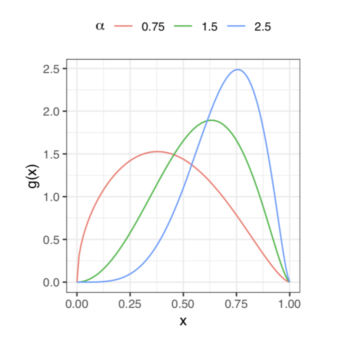
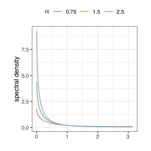
Figure 1: [left] Probability density $g(x)$, $x\in(0,1)$, in (27) for $\beta=2.5$. [right] Spectral density $f(\lambda)$, $\lambda\in[0,\pi]$, in (29) for the same value of $\beta$.

Let us turn to the description of our simulation procedure. We simulate 5000 panels for each configuration of $N$, $T$, $\alpha$ and $\beta$, where

• $(N,T)=(750,1000),\,(750,2000)$,

• $\beta=1.5,\,1.75,\,2,\,2.25,\,2.5$,

• $\alpha=0.75,\,1.5,\,2.5$.

As usual in tail-index estimation, the most difficult and delicate task is choosing the threshold. We note that conditions in Theorem 1 and Corollary 4 hold asymptotically and allow for different choice of $\delta$; moreover, they depend on (unknown) $\beta$ and the second-order parameter $\nu$. Roughly speaking, larger $\delta$ increases the number of the usable observations (upper order statistics) in (10) and (9), hence makes standard deviation of the estimator smaller, but at the same time increases bias since the density $g(x)$ in (2) is more likely to deviate from its asymptotic form on a longer interval $(1-\delta,1)$. In the i.i.d. case or $\beta_{N}$, the ‘optimal’ choice of $\delta$ is given by

$$\delta^{*}:=\Big{(}\frac{\beta(\beta+\nu)^{2}}{2\tau^{2}\nu^{3}\kappa N}\Big{)}^{1/(\beta+2\nu)},$$ (30)

see equation (4.3.8) in Goldie and Smith  (1987), which minimizes the asymptotic mean squared error of $\beta_{N}$ provided the distribution of $a_{i}$ satisfies a generally stronger version of the second-order condition in (6):

$$\mathbb{P}(a_{i}>1-x)=\kappa x^{\beta}(1+\tau x^{\nu}+o(x^{\nu})),\quad x\to 0+,$$ (31)

for the same $\beta>1$ and some parameters $\nu>0$, $\kappa>0$, $\tau\neq 0$. Then on average the computation of $\beta_{N}$ uses

$$\mathbb{E}\sum_{i=1}^{N}{\bf 1}(a_{i}>1-\delta^{*})\sim\Big{(}\frac{(1-\rho)N^{-\rho}}{B\sqrt{-2\rho}}\Big{)}^{2/(1-2\rho)}=:k^{*}$$ (32)

upper order statistics of $a_{1},\dots,a_{N}$, where the second-order parameters $\rho:=-\nu/\beta<0$, $B:=(\nu/\beta)\kappa^{-\nu/\beta}{\color[rgb]{0,0,1}\tau}\neq 0$ are more convenient to estimate, see e.g. Paulauskas and Vaičiulis  (2017). Therefore, given the order statistics $a_{(1)}\leq\dots\leq a_{(N)}$, we use (random) $\delta=1-a_{(N-\lfloor k^{*}\rfloor)}$ as a substitute for $\delta^{*}$. Furthermore, since $\delta^{*}$ of (30) yields asymptotic normality of $\beta_{N}$ in (9) with non-zero mean, we choose a smaller sample fraction $(k^{*})^{\epsilon}<k^{*}$ with $\epsilon\in(0,1)$ and the corresponding

$$\delta=1-a_{(N-\lfloor(k^{*})^{\epsilon}\rfloor)},$$ (33)

for which the asymptotic normality of $\beta_{N}$ holds as in Theorem 1. In our simulations of $\beta_{N}$ in (9) we use $\delta$ in (33) with several values of $\epsilon\in(0,1)$ and $k^{*}$ is obtained by replacing $\rho$, $B$ in (32) by their semiparametric estimates, see Fraga Alves et al.  (2003), Gomes and Martins  (2002). We calculate the latter estimates from $a_{1},\dots,a_{N}$ using the algorithm in Gomes et al.  (2009). Because of the lack of the explicit formula minimizing the mean squared error of $\widetilde{\beta}_{N}$, in our simulations of the latter estimator we use a similar threshold $\delta\in(0,1)$, viz.,

$$\delta=1-\widehat{a}_{(N-\lfloor(\widehat{k}^{*})^{\epsilon}\rfloor)},$$ (34)

where $\widehat{a}_{(1)}\leq\dots\leq\widehat{a}_{(N)}$ denote the order statistics calculated from the simulated RCAR(1) panel, and $\widehat{k}^{*}$ is the analogue of $k^{*}$ computed from $\widehat{a}_{1},\dots,\widehat{a}_{N}$. Moreover, for our simulations of $\widetilde{\beta}_{N}$ we use $r=10$ in (11), though any large $r$ could be chosen.

Table 1 illustrates the effect of $\epsilon$ in (33), (34) on the performance of $\beta_{N}$, $\widetilde{\beta}_{N}$, respectively, for $(N,T)=(750,1000)$. Choosing smaller $\epsilon$, the bias of the estimators decreases in most cases, whereas their standard deviation increases. The choice $\epsilon=0.9$ seems to be near ‘optimal’ in the sense of RMSE.

		$\beta=1.5$				$\beta=2$				$\beta=2.5$
$\epsilon$	$\alpha=$	0.75	1.5	2.5		0.75	1.5	2.5		0.75	1.5	2.5
		RMSE of $\widetilde{\beta}_{N}$
1		0.18	0.12	0.11		0.22	0.24	0.24		0.36	0.40	0.42
0.9		0.18	0.15	0.18		0.19	0.21	0.20		0.29	0.33	0.34
0.8		0.17	0.23	0.30		0.21	0.24	0.25		0.29	0.33	0.33
0.7		0.25	0.35	0.47		0.29	0.33	0.36		0.36	0.40	0.41
		RMSE of $\beta_{N}$
1		0.15	0.18	0.19		0.26	0.29	0.31		0.38	0.43	0.47
0.9		0.13	0.16	0.16		0.21	0.25	0.26		0.31	0.36	0.39
0.8		0.16	0.18	0.19		0.22	0.25	0.27		0.31	0.35	0.37
0.7		0.21	0.24	0.24		0.28	0.31	0.33		0.36	0.41	0.42
		Bias of $\widetilde{\beta}_{N}$
1		-0.07	-0.05	-0.01		-0.19	-0.20	-0.20		-0.32	-0.36	-0.38
0.9		-0.01	0.04	0.10		-0.11	-0.10	-0.08		-0.21	-0.25	-0.25
0.8		0.05	0.13	0.22		-0.04	-0.01	0.02		-0.13	-0.15	-0.13
0.7		0.11	0.23	0.36		0.02	0.07	0.12		-0.05	-0.06	-0.03
		Bias of $\beta_{N}$
1		-0.12	-0.14	-0.15		-0.23	-0.26	-0.28		-0.35	-0.40	-0.44
0.9		-0.06	-0.08	-0.09		-0.15	-0.17	-0.19		-0.24	-0.29	-0.32
0.8		-0.03	-0.04	-0.04		-0.09	-0.11	-0.12		-0.17	-0.21	-0.22
0.7		0.00	0.00	0.00		-0.05	-0.05	-0.06		-0.10	-0.13	-0.14

Table 1: Performance of $\widetilde{\beta}_{N}$, $\beta_{N}$ for $(N,T)=(750,1000)$, $a_{i}^{2}\sim\operatorname{Beta}(\alpha,\beta)$, using $\delta$ in (34), (33), respectively, with estimated parameters $B,\rho$ and $r=10$. The number of replications is $5000$.

Table 2 presents the performance of $\widetilde{\beta}_{N}$ and $\beta_{N}$ with $\epsilon=0.9$, for a wider choice of parameters $\alpha,\beta$ and two values of $T$. We see that the sample RMSE of both statistics $\widetilde{\beta}_{N}$ and $\beta_{N}$ are very similar almost uniformly in $\alpha,\beta,T$ (the only exception seems the case $\alpha=2.5,\beta=1.25,T=1000$). Surprisingly, in most cases the statistic $\widetilde{\beta}_{N}$ for $T=1000$ seems to be more accurate than the same statistic for $T=2000$ and the ‘i.i.d.’ statistic $\beta_{N}$. This unexpected effect can be explained by a positive bias introduced by estimated $a_{i}$ for $\epsilon=0.9$ which partly compensates the negative bias of $\beta_{N}$, see Table 2.

		$\beta=1.25$				$\beta=1.5$				$\beta=1.75$
	$\alpha=$	0.75	1.5	2.5		0.75	1.5	2.5		0.75	1.5	2.5
		RMSE
$\widetilde{\beta}_{N},\,T=1000$		0.11	0.17	0.27		0.18	0.15	0.18		0.15	0.16	0.17
$\widetilde{\beta}_{N},\,T=2000$		0.10	0.12	0.15		0.12	0.14	0.14		0.16	0.17	0.17
$\beta_{N}$		0.10	0.12	0.13		0.13	0.16	0.16		0.17	0.20	0.21
		Bias
$\widetilde{\beta}_{N},\,T=1000$		0.04	0.12	0.23		-0.01	0.04	0.10		-0.05	-0.03	0.00
$\widetilde{\beta}_{N},\,T=2000$		0.00	0.04	0.09		-0.04	-0.02	0.01		-0.08	-0.08	-0.07
$\beta_{N}$		-0.04	-0.05	-0.06		-0.06	-0.08	-0.09		-0.10	-0.12	-0.14
		$\beta=2$				$\beta=2.25$				$\beta=2.5$
	$\alpha=$	0.75	1.5	2.5		0.75	1.5	2.5		0.75	1.5	2.5
		RMSE
$\widetilde{\beta}_{N},\,T=1000$		0.19	0.21	0.20		0.23	0.26	0.26		0.29	0.33	0.34
$\widetilde{\beta}_{N},\,T=2000$		0.20	0.22	0.23		0.24	0.28	0.29		0.30	0.34	0.36
$\beta_{N}$		0.21	0.25	0.26		0.26	0.30	0.32		0.31	0.36	0.39
		Bias
$\widetilde{\beta}_{N},\,T=1000$		-0.11	-0.10	-0.08		-0.16	-0.17	-0.17		-0.21	-0.25	-0.25
$\widetilde{\beta}_{N},\,T=2000$		-0.12	-0.14	-0.14		-0.17	-0.20	-0.21		-0.23	-0.27	-0.28
$\beta_{N}$		-0.15	-0.17	-0.19		-0.19	-0.23	-0.25		-0.24	-0.29	-0.32

Table 2: Performance of $\widetilde{\beta}_{N}$, $\beta_{N}$ for $(N,T)=(750,1000)$ and $(N,T)=(750,2000)$, $a_{i}^{2}\sim\operatorname{Beta}(\alpha,\beta)$, using $\delta$ in (34), (33), respectively, with estimated parameters $B,\rho$ and $\epsilon=0.9$, $r=10$. The number of replications is $5000$.

Next, we examine the performance of the test statistics $\widetilde{Z}_{N}$ and $Z_{N}$ using $\delta$ in (34) and (33), respectively. Tables 3, 4 reports rejection rates of $H_{0}:\beta\geq 2$ in favour of $H_{1}:\beta<2$ at level $\omega=5\%$ using $\widetilde{Z}_{N}$ and $Z_{N}$ for $(N,T)=(750,2000)$ and different values of $\alpha,\beta$ and $\epsilon$, $r$. The results are almost the same when using $\widetilde{Z}_{N}$ for $r=3$ and $r=10$. Table 3 shows that choosing $\epsilon=0.7$ for $\beta\geq 2.25$ and all values of $\alpha$, the incorrect rejection rates of the null in favour of the long memory alternative are much smaller than $5\%$, despite the spurious long memory in Figure 1 [right]. Choosing $\epsilon=0.9$, they increase a bit but are still smaller than 5% using $\widetilde{Z}_{N}$, see Table 4. However, at the boundary $\beta=2$ between short and long memory, the empirical size of the tests is not well observed. The deviation from the nominal level is especially noticeable in the case of the ‘i.i.d.’ statistic $Z_{N}$. This size distortion may be explained by the fact that the tails of the empirical distribution of $Z_{N}$ and $\widetilde{Z}_{N}$ are not well-approximated by tails of the limiting normal distribution. More extensive simulations of the performance of $\widetilde{Z}_{N}$ and $Z_{N}$ for other choices of $\epsilon$, $r$, $N$, $T$ are presented in the arXiv version Leipus et al.  (2018) of this paper.

		$\beta=1.25$				$\beta=1.5$				$\beta=1.75$
	$\alpha=$	0.75	1.5	2.5		0.75	1.5	2.5		0.75	1.5	2.5
$\widetilde{Z}_{N}$, $r=3$		93.5	76.4	56.2		67.1	50.7	37.6		29.1	23.2	18.6
$\widetilde{Z}_{N}$, $r=10$		93.5	76.4	56.2		67.1	50.7	37.6		29.2	23.2	18.6
$Z_{N}$		97.0	94.0	93.5		76.8	69.6	68.7		36.7	35.7	35.8
		$\beta=2$				$\beta=2.25$				$\beta=2.5$
	$\alpha=$	0.75	1.5	2.5		0.75	1.5	2.5		0.75	1.5	2.5
$\widetilde{Z}_{N}$, $r=3$		7.8	7.9	6.1		0.8	1.5	1.8		0.1	0.2	0.4
$\widetilde{Z}_{N}$, $r=10$		8.0	7.9	6.1		0.9	1.5	1.8		0.1	0.2	0.4
$Z_{N}$		10.8	11.6	12.3		1.7	2.6	3.0		0.2	0.2	0.6

Table 3: Rejection rates (in %) of $H_{0}:\beta\geq 2$ at level $\omega=5\%$ with $\widetilde{Z}_{N}$, $Z_{N}$ for $(N,T)=(750,2000)$, $a_{i}^{2}\sim{\operatorname{Beta}}(\alpha,\beta)$, using $\delta$ in (34), (33), respectively, with estimated parameters $B$, $\rho$ and $\epsilon=0.7$. The number of replications is $5000$.

		$\beta=1.25$				$\beta=1.5$				$\beta=1.75$
	$\alpha=$	0.75	1.5	2.5		0.75	1.5	2.5		0.75	1.5	2.5
$\widetilde{Z}_{N}$, $r=3$		100.0	99.9	99.3		98.5	95.3	91.9		72.9	68.3	62.9
$\widetilde{Z}_{N}$, $r=10$		100.0	99.9	99.3		98.7	95.3	91.9		76.1	68.4	62.9
$Z_{N}$		100.0	99.9	99.9		99.2	97.9	97.6		81.0	78.1	78.1
		$\beta=2$				$\beta=2.25$				$\beta=2.5$
	$\alpha=$	0.75	1.5	2.5		0.75	1.5	2.5		0.75	1.5	2.5
$\widetilde{Z}_{N}$, $r=3$		19.8	25.1	23.8		1.1	4.2	4.6		0.0	0.3	0.6
$\widetilde{Z}_{N}$, $r=10$		26.7	25.5	23.8		2.2	4.4	4.6		0.1	0.3	0.6
$Z_{N}$		32.2	34.1	37.0		3.6	5.8	8.0		0.1	0.5	1.2

Table 4: Rejection rates (in %) of $H_{0}:\beta\geq 2$ at level $\omega=5\%$ with $\widetilde{Z}_{N}$, $Z_{N}$ for $(N,T)=(750,2000)$, $a_{i}^{2}\sim{\operatorname{Beta}}(\alpha,\beta)$, using $\delta$ in (34), (33), respectively, with estimated parameters $B$, $\rho$ and $\epsilon=0.9$. The number of replications is $5000$.

Remark 2.

In time series theory, several semi-parametric tests for long memory were developed, see Giraitis et al.  (2003), Gromykov et al.  (2018), Lobato and Robinson  (1998). Clearly, these tests cannot be applied to individual RCAR(1) series, the latter being always short memory a.s., independently of the value of $\beta$ and the distribution of the AR coefficient $a_{i}$. However, in practice one can apply the above-mentioned tests to the aggregated RCAR(1) series $\{\bar{X}_{N}(1),\dots,\bar{X}_{N}(T)\}$ in (4) whose autocovariance decays as $t^{-(\beta-1)}$, $t\to\infty$, see (3). In Leipus et al.  (2018) we report a Monte Carlo analysis of the finite sample performance of the V/S test (see Giraitis et al.  (2003)) applied to the aggregated RCAR(1) series with short memory $(\beta=2.5)$ for the same model as above. Since the V/S statistic is quite sensitive to the choice of the tuning parameter, Leipus et al.  (2018) derived its data-driven choice by expanding the HAC estimator as proved by Abadir et al.  (2009) and minimizing its mean squared error under the null hypothesis. The simulations in Leipus et al.  (2018) show that the V/S test is not valid, in the sense that its empirical size is not close to the nominal level. The reason why the V/S test fails for our panel model may be due to the presence of the spurious long memory (see Figure 1).

5 Proofs

Notation. In what follows, let $G_{N}(x):=N^{-1}\sum_{i=1}^{N}{\bf 1}(a_{i}\leq x)$ and $\widehat{G}_{N}(x):=N^{-1}\sum_{i=1}^{N}{\bf 1}(\widehat{a}_{i}\leq x)$, where $\widehat{a}_{1},\dots,\widehat{a}_{N}$ are defined by (5) and $a_{1},\dots,a_{N}$ are i.i.d. with $G(x):=\mathbb{P}(a_{1}\leq x)$, $x\in\mathbb{R}$.

Proof of Theorem 1.

We rewrite the estimator in (9) as

$$\beta_{N}=\frac{1-G_{N}(1-\delta)}{\int_{1-\delta}^{1}\ln(\delta/(1-x))\mathrm{d}G_{N}(x)}=\frac{1-G_{N}(1-\delta)}{\int_{1-\delta}^{1}(1-G_{N}(x))\frac{\mathrm{d}x}{1-x}}=\frac{1-G_{N}(1-\delta)}{\int_{0}^{\delta}(1-G_{N}(1-x))\frac{\mathrm{d}x}{x}}.$$

Next, we decompose $\beta_{N}-\beta=D^{-1}\sum_{i=1}^{4}I_{i}$, where

$$I_{1} := \beta\int_{0}^{\delta}(G_{N}(1-x)-G(1-x))\frac{\mathrm{d}x}{x},\qquad I_{2}:=-(G_{N}(1-\delta)-G(1-\delta)),$$ (35)

$$I_{3} := -\beta\int_{0}^{\delta}(1-\kappa x^{\beta}-G(1-x))\frac{\mathrm{d}x}{x},\qquad I_{4}:=1-\kappa\delta^{\beta}-G(1-\delta)$$

and

$$D:=\int_{0}^{\delta}(1-G_{N}(1-x))\frac{\mathrm{d}x}{x}=\frac{1}{\beta}(\kappa\delta^{\beta}-I_{1}-I_{3}).$$ (36)

According to the assumptions $(N\delta^{\beta})^{1/2}\delta^{\nu}\to 0$ and (G), we get $(N\delta^{-\beta})^{1/2}I_{4}\to 0$ and $(N\delta^{-\beta})^{1/2}I_{3}\to 0$.

From the tail empirical process theory, see e.g. Theorem 1 in Einmahl  (1990), (1.1)–(1.3) in Mason  (1988), we have that

$$(N\delta^{-\beta})^{1/2}(G_{N}(1-x\delta)-G(1-x\delta))\to_{D[0,1]}\kappa^{1/2}B(x^{\beta}),$$ (37)

where $\{B(x),\ x\in[0,1]\}$ is a standard Brownian motion. Therefore, we can expect that

$$(N\delta^{-\beta})^{1/2}(I_{1}+I_{2})\to_{d}\kappa^{1/2}\Big{(}\beta\int_{0}^{1}B(x^{\beta})\frac{\mathrm{d}x}{x}-B(1)\Big{)}.$$ (38)

The main technical point to prove (38) is to justify the application of the invariance principle (37) to the integral $(N\delta^{-\beta})^{1/2}I_{1}$, which is not a continuous functional in the uniform topology on the whole space $D[0,1]$. For $\varepsilon>0$, we split $I_{1}:=\beta(I_{0}^{\varepsilon}+I_{\varepsilon}^{1})$, where

$$I_{0}^{\varepsilon}:=\int_{0}^{\varepsilon}(G_{N}(1-\delta x)-G(1-\delta x))\frac{\mathrm{d}x}{x},\quad I_{\varepsilon}^{1}:=\int_{\varepsilon}^{1}(G_{N}(1-\delta x)-G(1-\delta x))\frac{\mathrm{d}x}{x}.$$

By (37), $(N\delta^{-\beta})^{1/2}I_{\varepsilon}^{1}\to_{d}\kappa^{1/2}\int_{\varepsilon}^{1}B(x^{\beta})\frac{\mathrm{d}x}{x}$, where $\mathbb{E}|\int_{\varepsilon}^{1}B(x^{\beta})\frac{\mathrm{d}x}{x}-\int_{0}^{1}B(x^{\beta})\frac{\mathrm{d}x}{x}|^{2}\to 0$ as $\varepsilon\to 0$. Hence, (38) follows from

$$\lim_{\varepsilon\to 0}\limsup_{N\to\infty}\mathbb{E}|(N\delta^{-\beta})^{1/2}I_{0}^{\varepsilon}|^{2}=0.$$ (39)

In the i.i.d. case $\mathbb{E}|I_{0}^{\varepsilon}|^{2}=\int_{0}^{\varepsilon}\int_{0}^{\varepsilon}\operatorname{Cov}(G_{N}(1-\delta x),G_{N}(1-\delta y))\frac{\mathrm{d}x\mathrm{d}y}{xy}$, where

$$\operatorname{Cov}(G_{N}(x),G_{N}(y))=N^{-1}G(x\wedge y)(1-G(x\vee y))\leq N^{-1}(1-G(x\vee y)),$$

and

$$\mathbb{E}|I_{0}^{\varepsilon}|^{2}\leq\frac{C}{N}\int_{0}^{\varepsilon}\frac{\mathrm{d}x}{x}\int_{0}^{x}(1-G(1-\delta y))\frac{\mathrm{d}y}{y}\leq\frac{C}{N}\int_{0}^{\varepsilon}\frac{\mathrm{d}x}{x}\int_{0}^{x}(\delta y)^{\beta}\frac{\mathrm{d}y}{y}=\frac{C}{N\delta^{-\beta}}\int_{0}^{\varepsilon}x^{\beta-1}\mathrm{d}x=\frac{C\varepsilon^{\beta}}{N\delta^{-\beta}},$$ (40)

proving (39) and hence (38) too.

Finally, we obtain $\delta^{-\beta}D\to_{p}\kappa/\beta$ in view of $(N\delta^{-\beta})^{1/2}(I_{1}+I_{3})=O_{p}(1)$ and $N\delta^{\beta}\to\infty.$

We conclude that

$$(N\delta^{\beta})^{1/2}(\beta_{N}-\beta)\to_{d}\frac{\beta}{\kappa^{1/2}}\Big{(}\beta\int_{0}^{1}B(x^{\beta})\frac{\mathrm{d}x}{x}-B(1)\Big{)}=:W.$$ (41)

Clearly, $W$ follows a normal distribution with zero mean and variance

$$\mathbb{E}W^{2}=\frac{\beta^{2}}{\kappa}\Big{(}2\beta^{2}\int_{0}^{1}\frac{\mathrm{d}x}{x}\int_{0}^{x}y^{\beta-1}\mathrm{d}y-2\beta\int_{0}^{1}x^{\beta-1}\mathrm{d}x+1\Big{)}=\frac{\beta^{2}}{\kappa},$$

which agrees with the one in Goldie and Smith  (1987). The proof is complete. ∎

In the proof of Theorem 2 we will use the following proposition.

Proposition 6.

Assume (G). As $N\to\infty$, let $\delta=\delta_{N}\to 0$ so that $N\delta^{\beta}\to\infty$ and (13), (14) hold. Then

$$(N\delta^{-\beta})^{1/2} (\widehat{G}_{N}(1-\delta)-G_{N}(1-\delta))=o_{p}(1),$$ (42)

$$(N\delta^{-\beta})^{1/2}\int_{\delta^{r}}^{\delta} (\widehat{G}_{N}(1-x)-G_{N}(1-x))\frac{\mathrm{d}x}{x}=o_{p}(1).$$ (43)

Proof.

For $x\in[1-\delta,1]$, write

$$\widehat{G}_{N}(x)-G_{N}(x)=\frac{1}{N}\sum_{i=1}^{N}({\bf 1}(a_{i}+\widehat{\rho}_{i}\leq x)-{\bf 1}(a_{i}\leq x))=D^{\prime}_{N}(x)-D^{\prime\prime}_{N}(x),$$

where $\widehat{\rho}_{i}:=\widehat{a}_{i}-a_{i}$, $i=1,\ldots,N$, and

$$D^{\prime}_{N}(x) := \frac{1}{N}\sum_{i=1}^{N}{\bf 1}(x<a_{i}\leq x-\widehat{\rho}_{i},\ \widehat{\rho}_{i}\leq 0),$$

$$D^{\prime\prime}_{N}(x) := \frac{1}{N}\sum_{i=1}^{N}{\bf 1}(x-\widehat{\rho}_{i}<a_{i}\leq x,\ \widehat{\rho}_{i}>0).$$

For all $\gamma>0$,

$$0\leq D^{\prime}_{N}(x)\leq\frac{1}{N}\sum_{i=1}^{N}{\bf 1}(x<a_{i}\leq x+\gamma\delta)+\frac{1}{N}\sum_{i=1}^{N}{\bf 1}(|\widehat{\rho}_{i}|>\gamma\delta)=:I^{\prime}_{N}(x)+I^{\prime\prime}_{N},$$

where by (13)

$$\mathbb{E}I^{\prime\prime}_{N}\leq\max_{1\leq i\leq N}\mathbb{P}(|\widehat{\rho}_{i}|>\gamma\delta)\leq\frac{\chi}{(\gamma\delta)^{p}}+\chi^{\prime}$$ (44)

and

$$\mathbb{E}I^{\prime}_{N}(x)=\mathbb{P}(x<a_{1}\leq x+\gamma\delta)\leq C\int_{x}^{x+\gamma\delta}(1-u)^{\beta-1}\mathrm{d}u\leq C\gamma\delta^{\beta}$$ (45)

holds uniformly for all $x\in[1-\delta,1]$ according to (6). Choose

$$\gamma:=\big{(}\frac{\chi}{\delta^{p+\beta}}\big{)}^{1/(p+1)},$$ (46)

then $\chi/(\gamma\delta)^{p}\sim\gamma\delta^{\beta}$ and the r.h.s. of (44) does not exceed $C(\gamma\delta^{\beta}+\chi^{\prime})\leq C\max\{\gamma\delta^{\beta},\chi^{\prime}\}$. Under the conditions (13), (14), from (44), (45) it follows that

$$(N\delta^{-\beta})^{1/2}\int_{\delta^{r}}^{\delta}\mathbb{E}D^{\prime}_{N}(1-x)\frac{\mathrm{d}x}{x}\leq C|\ln\delta|(N\delta^{-\beta})^{1/2}\big{(}\mathbb{E}I^{\prime\prime}_{N}+\sup_{x\in[0,\delta]}\mathbb{E}I^{\prime}_{N}(1-x)\big{)}=o(1),$$

hence

$$(N\delta^{-\beta})^{1/2}\int_{\delta^{r}}^{\delta}D^{\prime}_{N}(1-x)\frac{\mathrm{d}x}{x}=o_{p}(1)$$

by Markov’s inequality. Since

$$(N\delta^{-\beta})^{1/2}\int_{\delta^{r}}^{\delta}D^{\prime\prime}_{N}(1-x)\frac{\mathrm{d}x}{x}=o_{p}(1)$$

is analogous, this proves (43). The same proof works for the relation (42). ∎

Proof of Theorem 2.

Rewrite

$$\widetilde{\beta}_{N}=\frac{1-\widehat{G}_{N}(1-\delta)}{\int_{\delta^{r}}^{\delta}(1-\widehat{G}_{N}(1-x))\frac{\mathrm{d}x}{x}}.$$

Split $\widetilde{\beta}_{N}-\beta=\widetilde{D}^{-1}(\sum_{i=1}^{4}I_{i}+\sum_{i=1}^{4}R_{i})$, where $I_{i}$, $i=1,\dots,4$, are defined in (35) and

$$R_{1} := \beta\int_{\delta^{r}}^{\delta}(\widehat{G}_{N}(1-x)-G_{N}(1-x))\frac{\mathrm{d}x}{x},\qquad R_{2}:=G_{N}(1-\delta)-\widehat{G}_{N}(1-\delta),$$

$$R_{3} := \beta\int_{0}^{\delta^{r}}(G(1-x)-G_{N}(1-x))\frac{\mathrm{d}x}{x},\qquad R_{4}:=\beta\int_{0}^{\delta^{r}}(1-G(1-x))\frac{\mathrm{d}x}{x}$$

and

$$\widetilde{D}:=\int_{\delta^{r}}^{\delta}(1-\widehat{G}_{N}(1-x))\frac{\mathrm{d}x}{x}=D-\frac{1}{\beta}(R_{1}+R_{3}+R_{4})$$

with $D$ given by (36). By Proposition 6, $(N\delta^{-\beta})^{1/2}R_{2}=o_{p}(1)$ and $(N\delta^{-\beta})^{1/2}R_{1}=o_{p}(1)$. In view of (40), we have $\mathbb{E}|(N\delta^{-\beta})^{1/2}R_{3}|^{2}\leq C\delta^{r\beta}=o(1)$ and so $(N\delta^{-\beta})^{1/2}R_{3}=o_{p}(1)$. Finally, $(N\delta^{-\beta})^{1/2}R_{4}=o(1)$ as $N\delta^{(2r-1)\beta}\to 0$. ∎

Proof of Corollary 4.

Let $\chi:=T^{-\min\{p-1,p/2\}}$, $\chi^{\prime}:=\chi^{1/\min\{p-1,p/2\}}=T^{-1}$. Then (19)–(20) agree with (14) and the result follows from Theorem 2. ∎

Proof of Corollary 5.

Let $K_{N}=\sum_{i=1}^{N}{\bf 1}(a_{i}>1-\delta)$. Since $\operatorname{Var}(K_{N})\leq N(1-G(1-\delta))$ and $N(1-G(1-\delta))\to\infty$, Markov’s inequality yields

$$\frac{K_{N}}{N(1-G(1-\delta))}\to_{p}1,$$

consequently, $(N\delta^{\beta})^{-1}K_{N}\to_{p}\kappa$. By Proposition 6, we have $(N\delta^{\beta})^{-1}(\widetilde{K}_{N}-K_{N})=o_{p}(1)$. We conclude that $(N\delta^{\beta})^{-1}\widetilde{K}_{N}\to_{p}\kappa$. ∎

Data availability statement

Data sharing is not applicable to this article as no new data were created or analysed in this study.

References

- Abadir et al. (2009) Abadir, K., Distaso, W. and Giraitis, L. 2009. Two estimators of the long-run variance: beyond short memory. Journal of Econometrics 150, 56–70.
- Arellano (2003) Arellano, M. 2003. Panel Data Econometrics. Oxford University Press.
- Baltagi (2015) Baltagi, B.H. 2015. The Oxford Handbook of Panel Data. Oxford Handbooks.
- Beran et al. (2010) Beran, J., Schützner, M. and Ghosh, S. 2010. From short to long memory: Aggregation and estimation. Computational Statistics and Data Analysis 54, 2432–2442.
- Celov et al. (2007) Celov, D., Leipus, R. and Philippe, A. 2007. Time series aggregation, disaggregation and long memory. Lithuanian Mathematical Journal 47, 379–393.
- Celov et al. (2010) Celov, D., Leipus, R. and Philippe, A. 2010. Asymptotic normality of the mixture density estimator in a disaggregation scheme. Journal of Nonparametric Statistics 22, 425–442.
- Einmahl (1990) Einmahl, J.H.J. 1990. The empirical distribution function as a tail estimator. Statistica Neerlandica 44, 79–82.
- Fraga Alves et al. (2003) Fraga Alves, M.I., Gomes, M.I. and de Haan, L. 2003. A new class of semi-parametric estimators of the second order parameter. Portugaliae Mathematica 60, 193–214.
- Giraitis et al. (2003) Giraitis L., Kokoszka P., Leipus R. and Teyssière G. 2003. Rescaled variance and related tests for long memory in volatility and levels. Journal of Econometrics 112, 256–294.
- Goldie and Smith (1987) Goldie, C.M. and Smith, R.L. 1987. Slow variation with remainder: theory and applications. The Quarterly Journal of Mathematics 38, 45–71.
- Gomes and Martins (2002) Gomes, M.I. and Martins, M.J. 2002. “Asymptotically unbiased” estimators of the tail index based on external estimation of the second order parameter. Extremes 5, 5–31.
- Gomes et al. (2009) Gomes, M.I., Pestana, D. and Caeiro, F. 2009. A note on the asymptotic variance at optimal levels of a bias-corrected Hill estimator. Statistics and Probability Letters 79, 295–303.
- Gonçalves and Gouriéroux (1988) Gonçalves, E. and Gouriéroux, C. 1988. Aggrégation de processus autoregressifs d’ordre 1. Annales d’Economie et de Statistique 12, 127–149.
- Granger (1980) Granger, C.W.J. 1980. Long memory relationship and the aggregation of dynamic models. Journal of Econometrics 14, 227–238.
- Gromykov et al. (2018) Gromykov G., Ould Haye, M. and Philippe, A. 2018. A frequency-domain test for long range dependence. Statistical Inference for Stochastic Processes 21, 513–526.
- Kim and Kokoszka (2019a) Kim, M. and Kokoszka, P. 2019a. Consistency of the Hill estimator for time series observed with measurement errors. Preprint. Available at https://www.researchgate.net/publication/330352018.
- Kim and Kokoszka (2019b) Kim, M. and Kokoszka, P. 2019b. Asymptotic normality of the Hill estimator applied to data observed with measurement errors. Preprint. Available at https://www.researchgate.net/publication/334119192.
- Ling and Peng (2004) Ling, S. and Peng, L. 2004. Hill’s estimator for the tail index of an ARMA model. Journal of Statistical Planning and Inference 123, 279–293.
- Leipus et al. (2006) Leipus, R., Oppenheim, G., Philippe, A. and Viano, M.-C. 2006. Orthogonal series density estimation in a disaggregation scheme. Journal of Statistical Planning and Inference 136, 2547–2571.
- Leipus et al. (2014) Leipus, R., Philippe, A., Puplinskaitė, D. and Surgailis, D. 2014. Aggregation and long memory: recent developments. Journal of Indian Statistical Association 52, 71–101.
- Leipus et al. (2016) Leipus, R., Philippe, A., Pilipauskaitė, V. and Surgailis, D. 2017. Nonparametric estimation of the distribution of the autoregressive coefficient from panel random-coefficient AR(1) data. Journal of Multivariate Analysis 153, 121–135.
- Leipus et al. (2018) Leipus, R., Philippe, A., Pilipauskaitė, V. and Surgailis, D. 2018. Testing for long memory in panel random-coefficient AR(1) data. Preprint. Available at arXiv:1710.09735v2 [math.ST].
- Lobato and Robinson (1998) Lobato, I.N. and Robinson, P.M. 1998. A nonparametric test for I(). The Review of Economic Studies 65(3), 475–495.
- Mason (1988) Mason, D.M. 1988. A strong invariance theorem for the tail empirical process Annales de l’Institut Henri Poincaré 24, 491–506.
- Nedényi and Pap (2016) Nedényi, F. and Pap, G. 2016. Iterated scaling limits for aggregation of random coefficient AR(1) and INAR(1) processes, Statistics and Probability Letters 118, 16–23.
- Novak and Utev (1990) Novak, S.Y. and Utev, S. 1990. On the asymptotic distribution of the ratio of sums of random variables. Siberian Mathematical Journal 31, 781–788.
- Oppenheim and Viano (2004) Oppenheim, G. and Viano, M.-C. 2004. Aggregation of random parameters Ornstein-Uhlenbeck or AR processes: some convergence results. Journal of Time Series Analysis 25, 335–350.
- Paulauskas and Vaičiulis (2017) Paulauskas, V. and Vaičiulis, M. 2017. Comparison of the several parametrized estimators for the positive extreme value index. Journal of Statistical Computation and Simulation 87, 1342–1362.
- Philippe et al. (2014) Philippe, A., Puplinskaitė, D. and Surgailis, D. 2014. Contemporaneous aggregation of triangular array of random-coefficient AR(1) processes. Journal of Time Series Analysis 35, 16–39.
- Pilipauskaitė and Surgailis (2014) Pilipauskaitė, V. and Surgailis, D. 2014. Joint temporal and contemporaneous aggregation of random-coefficient AR(1) processes. Stochastic Process and their Applications 124, 1011–1035.
- Pilipauskaitė and Surgailis (2015) Pilipauskaitė, V. and Surgailis, D. 2015. Joint aggregation of random-coefficient AR(1) processes with common innovations. Statistics and Probability Letters 101, 73–82.
- Puplinskaitė and Surgailis (2009) Puplinskaitė, D. and Surgailis, D. 2009. Aggregation of random coefficient AR(1) process with infinite variance and common innovations. Lithuanian Mathematical Journal 49, 446–463.
- Puplinskaitė and Surgailis (2010) Puplinskaitė, D. and Surgailis, D. 2010. Aggregation of random coefficient AR(1) process with infinite variance and idiosyncratic innovations. Advances in Applied Probability 42, 509–527.
- Resnick and Stărică (1997) Resnick, S. and Stărică, C. 1997. Asymptotic behavior of Hill’s estimator for autoregressive data. Communications in Statistics. Stochastic Models 13, 703–721.
- Robinson (1978) Robinson, P.M. 1978. Statistical inference for a random coefficient autoregressive model. Scandinavian Journal of Statistics 5, 163–168.
- Zaffaroni (2004) Zaffaroni, P. 2004. Contemporaneous aggregation of linear dynamic models in large economies. Journal of Econometrics 120, 75–102.