Floquet Many-body Engineering: Topological and Many-body Physics in Phase Space Lattices

Abstract

Hamiltonians which are inaccessible in static systems can be engineered in periodically driven many-body systems, i.e., Floquet many-body systems. We propose to use interacting particles in a one-dimensional (1D) harmonic potential with periodic kicking to investigate two-dimensional (2D) topological and many-body physics. Depending on the driving parameters, the Floquet Hamiltonian of single kicked harmonic oscillator has various lattice structures in phase space. The noncommutative geometry of phase space gives rise to the topology of the system. We investigate the effective interactions of particles in phase space and find that the point-like contact interaction in quasi-1D real space becomes a long-rang Coulomb-like interaction in phase space, while the hardcore interaction in pure-1D real space becomes a confinement quark-like potential in phase space. We also find that the Floquet exchange interaction does not disappear even in the classical limit, and can be viewed as an effective long-range spin-spin interaction induced by collision. Our proposal may provide platforms to explore new physics and exotic phases by Floquet many-body engineering.

I Introduction

Since the concept of topological order was first introduced into condensed matter physics in 1973 Kosterlitz and Thouless (1973), topological phenomena have been intensively investigated in the past decades. Today, topology lies at the heart of many research fields, e.g., quantum Hall physics Hansson et al. (2017), topological insulators/superconductors Hasan and Kane (2010); Qi and Zhang (2011), and many more. The origin of topology in physics comes from the geometric phase factor of a quantum state when it moves along an enclosed path. In quantum Hall physics, the geometric phase is induced by the applied magnetic field and the resulting energy spectrum, also called the Hofstadter’s butterfly Hofstadter (1976), is a fractal; while the band can be characterized by its topological invariant (Chern number or TKNN invariant), which relates to the quantized Hall conductance directly Thouless et al. (1982). In topological insulators/superconductors, the spin-orbit coupling takes the role of an effective magnetic field Kane and Mele (2005); Bernevig et al. (2006) resulting in the geometric quantum phase factor. For the ultracold atoms in optical lattice Blochg (2005); Bloch et al. (2008), the geometric quantum phase (Berry phase Berry (1984)) is generated by shaking the lattice, which creates an artificial gauge field Jaksch and Zoller (2003); Goldman et al. (2009); Bermudez et al. (2010); Dalibard et al. (2011); Goldman et al. (2014); Aidelsburger (2016).

An alternative way to study topological physics is employing the noncommutativity of phase space in quantum mechanics. In a noncommutative space, the concept of point is meaningless due to the commutative relationship $[\hat{X},\hat{P}]=i\lambda$. Instead, we should define a coherent state $|\alpha\rangle$ which is the eigenstate of the lowering operater, i.e., $\hat{a}|\alpha\rangle=\alpha|\alpha\rangle$ with $\hat{a}\equiv(\hat{X}+i\hat{P})/\sqrt{2\lambda}$. As shown in Fig. 1, we observe that a coherent state moving along a closed path in phase space naturally acquires an additional quantum phase factor $e^{iS/\lambda}$, where $S$ is the enclosed area Pechal et al. (2012). This observation reveals the origin of topology in the study of many dynamical systems, e.g., the kicked harmonic oscillator (KHO) Zaslavsky (2008); Zaslavsky et al. (1986); Berman et al. (1991); Carvalho and Buchleitner (2004) and the kicked Harper model (KHM) Artuso et al. (1992, 1994). The energy spectra of these dynamical systems exhibit butterfly structure and band topology similar to quantum Hall systems Billam and Gardiner (2009); Geisel et al. (1991). In the strong kicking strength regime, the dynamical systems become chaotic and exhibits many novel behaviors such as dynamical localization, which has an intimate relation with the topology of bands Leboeuf et al. (1990, 1992); Dana (2014).

In many-body physics of equilibrium systems, many exotic phases of matter emerge when interaction makes the system strongly correlated. It is the interplay between topology and interaction that gives rise to the fractional quantum Hall effect Tsui et al. (1982); Laughlin (1983); Stormer (1999), and many other fascinating phenomena Callaway (1991); Tang et al. (2011); Neupert et al. (2011); Venderbos et al. (2012), like fractional charge and anyons Leinaas and Myrheim (1977); Wilczeks (1982); Wen (1991); Camino et al. (2005); Stern (2010); Khare (2005). Alternatively, it is also possible to engineer novel phases in periodically driven systems, i.e., the Floquet systems. The Hamiltonian of a Floquet system is a periodic function in time, i.e., $H(t)=H(t+T)$. The Floquet theory Shirley (1965); Grifoni and Hänggi (1998) allows us to describe stroboscopic time-evolution for every period by a time-independent Hamiltonian which is called the Floquet Hamiltonian $H_{F}$ and is defined by $e^{-\frac{i}{\hbar}TH_{F}}\equiv\mathcal{T}e^{-\frac{i}{\hbar}\int_{0}^{T}H(t)dt}$, or equivalently

$$H_{F}=i\frac{\hbar}{T}\mathrm{ln}\Big{[}\mathcal{T}e^{-\frac{i}{\hbar}\int_{0}^{T}H(t)dt}\Big{]}.$$ (1)

Here, $T$ is the chosen stroboscopic time step and $\mathcal{T}$ is the time-ordering operator. Exotic Floquet Hamiltonians Rahav et al. (2003a, b); Verdeny et al. (2013); Bandyopadhyay and Sarkar (2015); Eckardt1 and Anisimovas (2015); Itin and Katsnelson (2015); Guo et al. (2016) which are inaccessible in static systems can be engineered from Eq. (1) and a range of novel physical phenomena, such as phase space crystals Guo et al. (2013); Guo and Marthaler (2016), Anderson localization (or many-body localization) in time domain Sacha (2015a); Sacha and Delande (2016); Giergiel and Sacha (2017); Mierzejewski et al. (2017) and spontaneous breaking of discrete time-translation symmetry (Floquet time crystals) Heo et al. (2010); Sacha (2015b); Else et al. (2016); Khemani et al. (2016); Yao et al. (2017); Zhang et al. (2017a); Choi et al. (2017); Sacha and Zakrzewski (2017); Zhang et al. (2017b), can be created by Floquet engineering Bukov et al. (2015); Holthaus (2016); Eckardt (2017). While most work focus on the single-particle physics of (dissipative) Floquet systems, the possible new physics by Floquet many-body engineering has become an active research direction in recent years. Unlike the static many-body systems, the generic nonintegrable Floquet many-body systems are expected to be heated up, by the driving field, to a trivial stationary state with infinite temperature D’Alessio and Rigol (2014); Lazarides et al. (2014); Pontea et al. (2015). However, before reaching the long-time featureless infinite-temperature state, there is a prethermal state with exponentially long lifetime for high driving frequencies, and therefore existing a prethermal dynamics which can be described by the time-independent Floquet Hamiltonian (1) Abanin et al. (2015); Mori et al. (2016); Abanin et al. (2017a); Kuwaharaa et al. (2016); Bukov et al. (2016); Canovi et al. (2016); Abanin et al. (2017b); Weidinger and Knap (2017); Ho et al. (2017); Machado et al. (2017). By introducing disorder as in many-body localized systems Bordia et al. (2017) or coupling the Floquet many-body system to a cold bath Else et al. (2017), it is also possible to protect the metastable prethermal state.

In this paper, we investigate cold atoms trapped in 1D harmonic potential with a stroboscopically applied optical lattice. The equation of motion of a single atom corresponds to the kicked harmonic oscillator (KHO) and we find that that intriguing 2D topological and many-body physics emerges in phase space. The Floquet Hamiltonian of a single KHO, in the rotating wave approximation (RWA), forms various lattice structures in phase space depending on the driving parameters. The full dissipative quantum dynamics shows that the stationary state forms a lattice structure in phase space but with a finite size limited by the dissipation rate. Furthermore, we consider the interaction between cold atoms and find that the point-like contact interaction of cold atoms in real space becomes a long-range Coulomb-like interaction in phase space. More interestingly, the hard-core interaction of cold atoms in real space becomes a long-range potential which increases linearly with the distance in phase space, i.e., a quark-like confinement potential. We also find the Floquet exchange interaction has Coulomb-like long-range behavior, which does not disappear in the classical limit and becomes an effective spin-spin interaction.

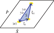
Figure 1: Geometric quantum phase in phase space. A coherent state $|\alpha\rangle$ is moved along a closed triangle by three displacement operators, i.e., $D[-(\xi_{1}+\xi_{2})]D(\xi_{2})D(\xi_{1})|\alpha\rangle=e^{i\frac{1}{\lambda}S}|\alpha\rangle,$ where $D(\xi)\equiv\exp(\frac{\xi}{\sqrt{2\lambda}}\hat{a}^{\dagger}-\frac{\xi^{*}}{\sqrt{2\lambda}}\hat{a})$ with two complex numbers $\xi_{1},\ \xi_{2}$ determining the moving path. The geometric phase factor is given by $e^{i\frac{1}{\lambda}S}$ with $S=\frac{1}{2}\mathrm{Im}[\xi_{2}\xi^{*}_{1}]$ being the area of the enclosed path (blue area).

II Model and Hamiltonian

We start from interacting cold atoms trapped by an elongated three-dimensional harmonic potential, with the radial motion cooled down to the ground state. In this way, the spatial motion of the atoms is restricted to the remaining axial direction. In general, the one-dimensional system is described by

$$H(t)=\sum_{i}H_{s}(\hat{x}_{i},\hat{p}_{i},t)+\sum_{i<j}V(\hat{x}_{i}-\hat{x}_{j}),$$ (2)

where $V(\hat{x}_{i}-\hat{x}_{j})$ is the two-body interaction, which is typically contact or hard-core interactions in the context of cold atoms Bloch et al. (2008); Olshanii (1998); Bergeman et al. (2003); Astrakharchik et al. (2004); Paredes et al. (2004); Kinoshita et al. (2004); Haller et al. (2009). The $H_{s}(\hat{x}_{i},\hat{p}_{i},t)$ is the single-particle Hamiltonian which can be explicitly time-dependent. Here, the single-particle Hamiltonian is the quantum kicked harmonic oscillator, which is described by $H_{s}=\frac{1}{2m}\hat{p}_{i}^{2}+\frac{1}{2}m\omega_{0}^{2}\hat{x}_{i}^{2}+K_{0}T_{d}\cos(k\hat{x}_{i})\sum_{n=-\infty}^{\infty}\,\delta(t-nT_{d}),$ where $\omega_{0}$ is the axial harmonic frequency and $m$ is the atom’s mass. The periodic term is implemented by a stroboscopic optical lattice, which can be created by two counter-propagating laser beams with off-resonant frequency far away from internal electronic transitions Blochg (2005); Bloch et al. (2008). Parameters $k$ and $K_{0}$ are the wave vector of the laser beams and the kicking strength, respectively. Parameter $T_{d}$ is the time period between adjacent kicking pluses. We scale the coordinate and momentum by the units of $\sqrt{\hbar/(\lambda m\omega_{0})}$ and $\sqrt{m\hbar\omega_{0}/\lambda}$ with the parameter $\lambda\equiv\hbar k^{2}/m\omega_{0}$, respectively. Finally, we have the dimensionless single-particle Hamiltonian scaled by $\hbar\omega_{0}/\lambda$

$$H_{s}(\hat{x}_{i},\hat{p}_{i},t)=\frac{1}{2}(\hat{x}_{i}^{2}+\hat{p}_{i}^{2})+K\tau\cos\hat{x}_{i}\sum_{n=-\infty}^{\infty}\,\delta(t-n\tau),$$ (3)

where $K=\lambda K_{0}/\hbar\omega_{0}$ is the dimensionless kicking strength, $\tau=\omega_{0}T_{d}$ is the dimensionless kicking period and the time $t$ has also been scaled by $\omega_{0}^{-1}$. The commutation relationship between the coordinate and the momentum is now $[\hat{x}_{i},\hat{p}_{j}]=i\lambda\delta_{ij}$, where the dimensionless parameter $\lambda$ plays the role of an effective Planck constant. Thus, the semiclassical regime corresponds to the limit $\lambda\rightarrow 0$. Accordingly, the two-body interaction will be given by the new scaled dimensionless observables as $V(\hat{x}_{i}-\hat{x}_{j})$.

Our remaining paper is organized as follows. In Sec. III, we discuss the single-particle physics neglecting interaction of paticles. We first introduce the topological band theory of phase space lattices in Sec. III.1. Then, in Sec III.2, we investigate the dissipative quantum dynamics of a KHO in a realistic environment and show how a lattice structure is formed in phase space. In Sec. IV, we consider the interactions and investigate the many-body dynamics. We first develop a general theory of transforming a given real space interaction potential to a phase space interaction potential in Sec IV.1. Then, in Sec IV.2, we apply our theory of phase space interaction to the special cases of contact interaction and hard-core interaction of cold atoms, and give the analytical expressions of corresponding phase space interactions. In Sec IV.3 and IV.4, we investigate the many-body dynamics in the classical limit and discuss the concept of dynamical crystals. Finally, we summarize our results in Sec. V.

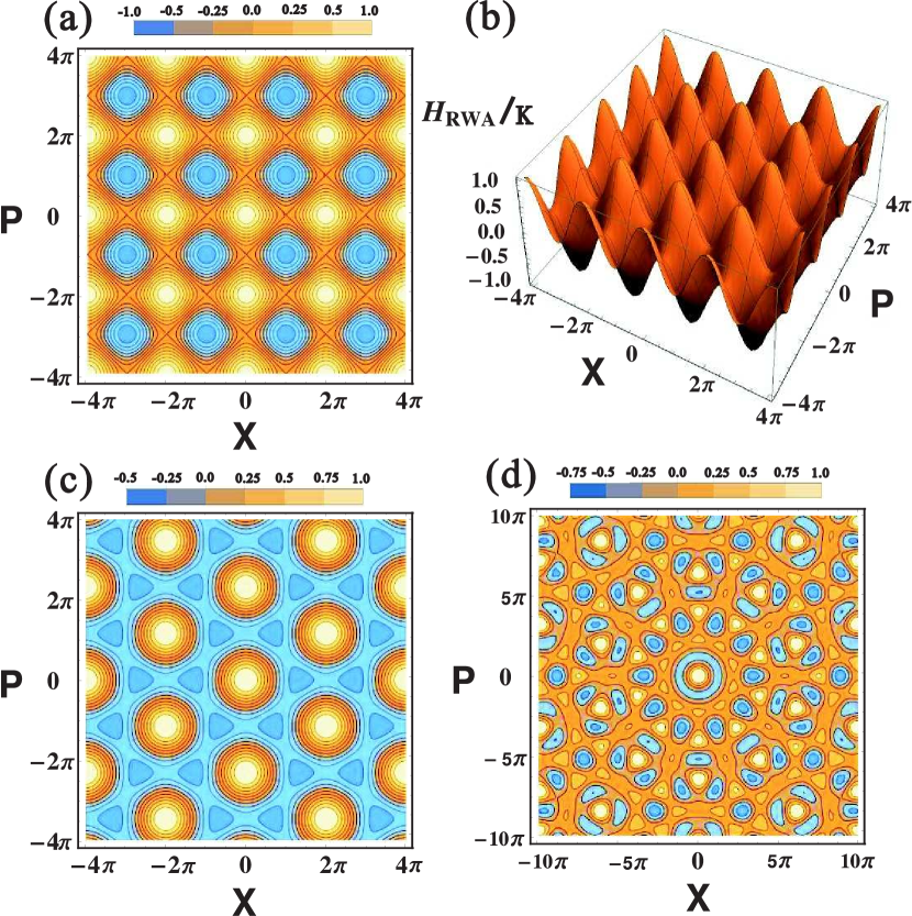
Figure 2: Phase space lattices: $H_{RWA}(X,P)$ for different $q_{0}$. (a) 2D density plot of square lattice for $q_{0}=4$. (b) 3D plot of square lattice for $q_{0}=4$. (c) Hexagonal lattice for $q_{0}=3$ or $q_{0}=6$. (d) Quasicrystal structures for $q_{0}=5$. The value of $H_{RWA}(X,P)$ has been scaled by the kicking strength $K$ in all figures.

III Phase Space Lattices

In this section, we investigate the single-particle Hamiltonian of the quantum KHO, i.e., Eq. (3), in the resonant condition that the kicking period satisfies $\tau=2\pi/q_{0}$ with $q_{0}$ an integer. When the kicking strength is weak $|K|\ll 1$, the single-particle dynamics is still dominated by the fast harmonic oscillation. Then we transform into an appropriately chosen rotating frame generated by the free time-evolution operator $\hat{O}(t)\equiv\exp(i\sum_{i}\hat{a}_{i}^{\dagger}\hat{a}_{i}t/\lambda)$, where $\hat{a}_{i}$ is the annihilation operator defined by $\hat{a}_{i}\equiv(\hat{x}_{i}+i\hat{p}_{i})/\sqrt{2\lambda}$. We transform the coordinates and momenta of particles by

$$\left\{\begin{array}[]{lll}\hat{O}(t)\hat{x}_{i}\hat{O}^{\dagger}(t)&=&\hat{P}_{i}\sin t+\hat{X}_{i}\cos t\\ \hat{O}(t)\hat{p}_{i}\hat{O}^{\dagger}(t)&=&\hat{P}_{i}\cos t-\hat{X}_{i}\sin t.\\ \end{array}\right.$$ (6)

Here, the operators $\hat{X}_{i}$ and $\hat{P}_{i}$ describe the dynamics of the $i$-th atom’s phase and amplitude. For the harmonic oscillator, $\hat{X}_{i}$ and $\hat{P}_{i}$ are fixed and correspond to the initial state of $\hat{x}_{i}(t)$ and $\hat{p}_{i}(t)$. In our case, however, the phase and amplitude of KHO are slightly changed every harmonic time period due to the weak kicking. The time-evolution of $\hat{X}_{i}$ and $\hat{P}_{i}$ is slow compared to the fast global harmonic oscillation and can be obtained stroboscopically from the time-evolution of $\hat{x}_{i}(t)$ and $\hat{p}_{i}(t)$ every time period of $2\pi$.

From Eq. (6), we have $[\hat{X}_{i},\hat{P}_{j}]=[\hat{x}_{i},\hat{p}_{j}]=i\lambda\delta_{ij}$. The canonical transformation of the single-particle Hamiltonian is given by $\hat{O}(t)H_{s}\hat{O}^{\dagger}(t)-iO(t)\dot{O}^{\dagger}(t)$. In RWA, we drop the fast oscillating terms and arrive at the time-independent Hamiltonian (see detailed derivation in Appendix A)

$$H_{\it RWA}(\hat{X},\hat{P})=\frac{K}{q_{0}}\sum_{j=1}^{q_{0}}\,\cos\left(\hat{X}\cos\frac{2\pi j}{q_{0}}+\hat{P}\sin\frac{2\pi j}{q_{0}}\right).$$ (7)

Here, we have dropped the index of the operators since we are considering single-particle physics. Another way of deriving $H_{\it RWA}(\hat{X},\hat{P})$ is based on the series expansion of the Floquet Hamiltonian (1) in order of the kicking strength $K$. By replacing the Planck constant $\hbar$ by a dimensionless one $\lambda$ and choosing the stroboscopic time step $T=q_{0}\tau$, we have the time-evolution operator in one stroboscopic time step $\mathcal{T}e^{-\frac{i}{\lambda}\int_{0}^{q_{0}\tau}H_{s}(t)dt}=\hat{F}^{q_{0}}$ with the Floquet operator for one period $\hat{F}\equiv e^{-i(\hat{x}^{2}+\hat{p}^{2})\tau/2\lambda}e^{iK\cos{\hat{x}}/\lambda}$. In the Appendix A, we show that $H_{\it RWA}(\hat{X},\hat{P})$ is indeed the first order expansion of the Floquet operator $\hat{F}^{q_{0}}$.

To display the symmetries of $H_{\it RWA}(\hat{X},\hat{P})$ in phase space, we calculate the averaged $H_{\it RWA}(\hat{X},\hat{P})$ in the coherent state representation (see the details in Appendix B), i.e.,

$$\langle\alpha|H_{\it RWA}(\hat{X},\hat{P})|\alpha\rangle=e^{-\lambda/4}H_{\it RWA}(X,P).$$

Here, the coherent state $|\alpha\rangle$ is defined by the eigenstate of the annihilation operator $\hat{a}\equiv(\hat{X}+i\hat{P})/\sqrt{2\lambda}$, i.e., $\hat{a}|\alpha\rangle=\alpha|\alpha\rangle$. The averaged position and momentum are $X\equiv\langle\alpha|\hat{X}|\alpha\rangle=\sqrt{2\lambda}\mathrm{Re}[\alpha]$ and $P\equiv\langle\alpha|\hat{P}|\alpha\rangle=\sqrt{2\lambda}\mathrm{Im}[\alpha]$. The quantity $H_{\it RWA}(X,P)$ has the same expression as Eq. (7) but replacing the operators $\hat{X}$ and $\hat{P}$ by the averaged values $X$ and $P$ respectively. In Fig. 2, we plot $H_{\it RWA}(X,P)$ in phase space for different $q_{0}$. We see that the $H_{\it RWA}(X,P)$ has a square lattice structure for $q_{0}=4$, hexagonal lattice structure for $q_{0}=3$ or $q_{0}=6$, and even quasicrystal structure for $q_{0}=5$ or $q_{0}\geq 7$. The translational symmetry of the Hamiltonian (7) in phase space gives rise to the band structure of its spectrum.

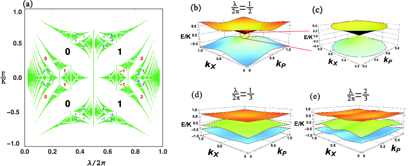
Figure 3: Quasienergy band structures. (a) Hofstadter’s butterfly: the quasienergy spectrum of Hamiltonian (8) with rational number $\lambda/2\pi\in[0,1]$. (b)-(e) Quasienergy band structures in 2D Brillouin zone for different parameters $\lambda$ which are given above the figures. For $\lambda/2\pi=1/2$, the two bands touch each other in the center of Brillouin zone. The linear dispersion relationship near the touching point is shown in figure (c).

III.1 Band Structure and Topology

We will deal with the case of square lattice ($q_{0}=4$) in detail but the results can be readily generalized to the case of hexagonal lattice ($q_{0}=3$ or $6$). For $q_{0}=4$, the effective Hamiltonian (7) is further simplified as

$$H_{sq}(\hat{X},\hat{P})=\frac{1}{2}K\Big{(}\cos\hat{X}+\cos\hat{P}\Big{)}.$$ (8)

This Hamiltonian is closely related to the established Harper’s equation, which is a tight binding model governing the motion of noninteracting electrons in the presence of a two-dimensional periodic potential and a uniformly threading magnetic field Harper (1955); Hofstadter (1976). The $H_{sq}(\hat{X},\hat{P})$ is invariant under discrete translation in phase space by two operators $\hat{T}_{1}\equiv e^{i\frac{2\pi}{\lambda}\hat{P}}$ and $\hat{T}_{2}\equiv e^{i\frac{2\pi}{\lambda}\hat{X}}$, i.e.,

$$\left\{\begin{array}[]{lll}\hat{T}_{1}H_{sq}(\hat{X},\hat{P})\hat{T}^{\dagger}_{1}=H_{sq}(\hat{X}+2\pi,\hat{P})=H_{sq}(\hat{X},\hat{P})\\ \hat{T}_{2}H_{sq}(\hat{X},\hat{P})\hat{T}^{\dagger}_{2}=H_{sq}(\hat{X},\hat{P}+2\pi)=H_{sq}(\hat{X},\hat{P}).\\ \end{array}\right.$$ (11)

The translation operators $\hat{T}_{1}$ and $\hat{T}_{2}$ generate an invariance group $G$ of $H_{sq}$ Dana (1995), which is a nonabelian group due to the identity $[\hat{T}^{r}_{1},\hat{T}^{s}_{2}]=\hat{T}_{1}\hat{T}_{2}(1-e^{-i4\pi^{2}rs/\lambda})$ with integer powers $r,s\in\mathbb{Z}$. However, the group $G$ has abelian subgroups $G_{a}$ generated by $\hat{T}_{1}^{r}$ and $\hat{T}_{2}^{s}$ if $2\pi rs/\lambda\in\mathbb{Z}$, which means the value of the parameter $\lambda/2\pi$ needs to be a rational number, i.e., $\lambda/2\pi=p/q$, where $p$ and $q$ are coprime integers. Here, we choose the abelian subgroup $G_{a}$ generated by the following two generators ($r=1$, $s=p$)

$$\hat{T}_{X}\equiv\hat{T}_{1}=e^{i\frac{2\pi}{\lambda}\hat{P}},\ \ \ \ \ \ \hat{T}_{P}\equiv\hat{T}^{p}_{2}=e^{i\frac{2\pi p}{\lambda}\hat{X}}.$$ (12)

Therefore, we can find the common eigenstates of commutative operators $\hat{T}_{X}$ and $\hat{T}_{P}$ with eigenvalues given by $e^{i2\pi k_{X}}$ and $e^{i2\pi pk_{P}}$ respectively. The boundaries of the two dimensional Brillouin zone are defined by $0\leq k_{X}\leq 1$ and $0\leq k_{P}\leq 1/p$, where $k_{X}$ and $k_{P}$ are quasimomentum and quasicoordinate, respectively Zak (1972). The corresponding eigenvalues of the Hamiltonian $H_{sq}$ are also called quasienergies.

The discrete translational symmetry in phase space allows us to determine the quasienergy spectrum numerically in Zak’s $kq$-representation (see the instruction in Appendix C or Ref. Zak (1972)). Given the parameters of $\lambda/2\pi=p/q$, $k_{X}$ and $k_{P}$, the eigenvalues $E$ of $H_{sq}$ are determined by the following polynomial equation (see the derivation in Appendix D or Ref. Butler and Brown (1968))

$$\cos(q\lambda k_{X})+\cos(q\lambda k_{P})=1+\frac{1}{2}\mathrm{Tr}\prod_{j=1}^{q}\begin{bmatrix}\frac{4E}{K}-2\cos(j\lambda)&-1\\ 1&0\end{bmatrix}.$$ (13)

The left hand side of Eq. (13) takes values in the range $[-2,2]$ when the quasimomentum $k_{X}$ and quasicoordinator $k_{P}$ run over the whole Brillouin zone. The right hand side of Eq. (13) is a periodic function of $\lambda$ with period $2\pi$. Therefore, the quasienergy spectrum is also a periodic function of $\lambda$ with period $2\pi$. In Fig. 3(a), we plot the quaienergy spectrum for $\lambda/2\pi\in[0,1]$, showing a Hofstadter butterfly structure identical to that in quantum Hall systems. In Fig. 3(b), (d) and (e), we plot the quasienergy band structures in the two-dimensional Brillouin zone $(k_{X},k_{p})$ for $\lambda/2\pi=1/2,1/3$ and $2/3$, respectively. For the given parameter $\lambda/2\pi=1/2$, we can obtain the analytical solutions from Eq. (13), i.e.,

$$E=\pm\frac{1}{2}K\sqrt{1+\frac{1}{2}(\cos 2\pi k_{X}+\cos 2\pi k_{P})}.$$

The two bands touch each other at the central point of the Brillouin zone, i.e., $(k_{X}=\frac{1}{2},k_{P}=\frac{1}{2})$, where the dispersion relationship becomes linear near the touching point, i.e., $E\approx\pm\frac{\pi K}{\sqrt{2}}|k|$ with $|k|\equiv\sqrt{(k_{X}-\frac{1}{2})^{2}+(k_{P}-\frac{1}{2})^{2}}$, as shown in Fig. 3(c). In general, the two innermost bands always touch each other for even integer $q$. We also see that the quasienergy band structure is two-fold degenerate for $\lambda/2\pi=2/3$ while there is no degeneracy for $\lambda/2\pi=1/2$ and $\lambda/2\pi=1/3$. In fact, for each rational $\lambda/2\pi=p/q$ (remembering $p,q$ are coprime integers), the spectrum contains $q$ bands and each band has a $p$-fold degeneracy due to the fact that the invariance group $G$ can be expressed as the coset sum $\sum_{r=1}^{p}\hat{T}_{1}^{r}G_{a}$ Dana (1995).

We denote the quasienergy states by $|\psi_{b,\mathbf{k}}\rangle$ with $\mathbf{k}\equiv(k_{X},k_{P})$ and $b$ the band index counting from the bottom. To visualize the quasienergy states, we define the Husimi $Q$-function of a given eigenstate in phase space Gerry and Knight (2004)

$$Q_{b,{\mathbf{k}}}(\alpha,\alpha^{*})\equiv\frac{1}{\pi}\langle\alpha|\psi_{b,{\mathbf{k}}}\rangle\langle\psi_{b,{\mathbf{k}}}|\alpha\rangle=\frac{1}{\pi}|\langle\alpha|\psi_{b,{\mathbf{k}}}\rangle|^{2}$$ (14)

where $|\alpha\rangle$ is the coherent state introduced at the beginning in this section. In Figs. 4(a) and (b), we plot the $Q$-functions of eigenstates $|\psi_{1,(0,0)}\rangle$ and $|\psi_{2,(0,0)}\rangle$ for $\frac{\lambda}{2\pi}=\frac{1}{2}$, which are the ground-like states of the lower band and upper band, respectively. Comparing the $Q$-functions of the two states to the phase space lattices shown in Fig. 2(a), we see that the $Q$-function of eigenstate $|\psi_{1,(0,0)}\rangle$ mostly occupies the negative phase space lattice $H_{sq}(X,P)<0$ while the $Q$-function of eigenstate $|\psi_{2,(0,0)}\rangle$ is shifted by $\pi$ along both $X$ and $P$ directions in phase space, mostly occupying the positive phase space lattice $H_{sq}(X,P)>0$. In fact, our system has a chiral symmetry defined by the chiral operator $\hat{T}_{c}\equiv e^{i\frac{\pi}{\lambda}\hat{X}}e^{i\frac{\pi}{\lambda}\hat{P}}$, i.e., $\hat{T}_{c}H_{sq}\hat{T}^{\dagger}_{c}=-H_{sq}$. Thus, for a given eigenstate $|\psi_{b,\mathbf{k}}\rangle$, there must be another eigenstate $\hat{T}^{\dagger}_{c}|\psi_{b,\mathbf{k}}\rangle$ with opposite quasienergy. In Figs. 4(c) and (d), we plot the $Q$-functions of eigenstates $|\psi_{1,(\frac{1}{4},\frac{1}{2})}\rangle$ and $|\psi_{1,(\frac{3}{4},\frac{1}{2})}\rangle$ for $\frac{\lambda}{2\pi}=\frac{2}{3}$, which are the degenerate states of the lower band shown in Fig. 3(e). We see that the period along $X$-direction is $2\pi$ while the period along $P$-direction is $4\pi$. In fact, this degeneracy depends on the discrete translation operators we choose in Eq. (12). For $\frac{\lambda}{2\pi}=\frac{p}{q}$, the period of any $Q$-function of eigenstate is $2\pi p$-period in $P$-direction and $2\pi$-period in $X$-direction. Theses $p$-degenerate states are given by

$$|\psi_{b,\mathbf{k}}\rangle,\ \hat{T}_{2}|\psi_{b,\mathbf{k}}\rangle,\ \hat{T}^{2}_{2}|\psi_{b,\mathbf{k}}\rangle,\ \cdot\cdot\cdot,\ \hat{T}^{p-1}_{2}|\psi_{b,\mathbf{k}}\rangle$$

with the same quasicoordinator but different quasimomenta. In the case of $\frac{\lambda}{2\pi}=\frac{2}{3}$, the two degenerate states of $|\psi_{b,\mathbf{k}}\rangle$ and $\hat{T}_{2}|\psi_{b,\mathbf{k}}\rangle$ in the $X$-representation are $\langle X|\psi_{b,\mathbf{k}}\rangle=\psi_{b,\mathbf{k}}(X)$ and $\langle X|\hat{T}_{2}|\psi_{b,\mathbf{k}}\rangle=e^{i\frac{2\pi}{\lambda}X}\psi_{b,\mathbf{k}}(X)$. Therefore, the $Q$-functions of the two degenerate states are the same in the $X$-dimension. But due to the relationship $\langle\psi_{b,\mathbf{k}}|\hat{P}|\psi_{b,\mathbf{k}}\rangle=\langle\hat{T}_{2}\psi_{b,\mathbf{k}}|\hat{P}|\hat{T}_{2}\psi_{b,\mathbf{k}}\rangle+2\pi$, the $Q$-functions are shifted by $2\pi$ in the $P$-dimension.

The underlying topology of a quasienergy band is defined by the Chern number Reynoso et al. (2017)

$$c_{b}=\oint_{\mathcal{C}}\langle\psi_{b,\mathbf{k}}|\partial_{\mathbf{k}}|\psi_{b,\mathbf{k}}\rangle\cdot d\mathbf{k},$$ (15)

where the contour $\mathcal{C}$ is integrated over the boundary of the Brillouin zone. The Chern number associated with a gap is subtle here. For the equilibrium systems, the Chern number of a gap is defined by the sum of the Chern numbers of the energy bands below the gap. However, in our present work, we are dealing with a Floquet system far from equilibrium. The general statistic law of the Floquet states for the long-time stationary state is an on-going research topic Hone et al. (2009); Ketzmerick and Wustmann (2010); Shirai et al. (2016). Actually, the positive and negative sublattices shown in Fig. 2(a) make no difference in the frame of Floquet theory. We assume that the statistic mechanics near the ground state of each sublattice can be described by an effective Floquet-Gibbs states Shirai et al. (2016). Therefore, we define the Chern number of a gap below (above) the zero energy line as the sum of Chern numbers of all the quasienergy bands below (above) the gap. As shown in Fig. 3(a), the Chern number of some gaps are calculated and labelled symmetrically with respect to zero energy line.

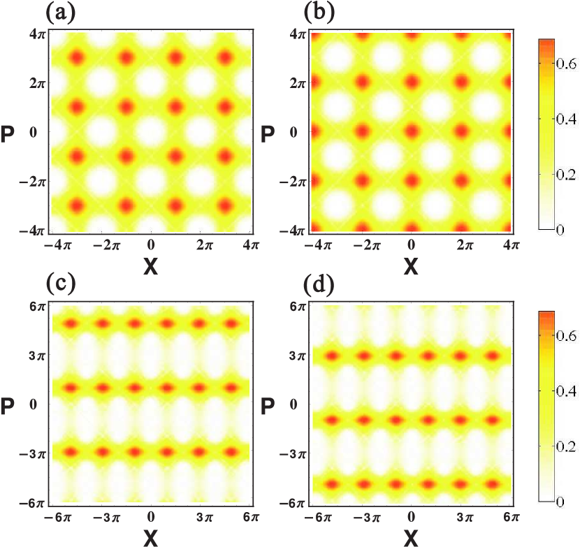
Figure 4: Husimi $Q$-functions of eigenstate $|\psi_{b,{\mathbf{k}}}\rangle$. (a) Eigenstate $|\psi_{1,(0,0)}\rangle$ with the minimum quasienergy of the lower band for $\frac{\lambda}{2\pi}=\frac{1}{2}$. (b) Eigenstate $|\psi_{2,(0,0)}\rangle$ with the maximum quasienergy of the upper band for $\frac{\lambda}{2\pi}=\frac{1}{2}$. (c) Eigenstate $|\psi_{1,(\frac{1}{4},\frac{1}{2})}\rangle$ for $\frac{\lambda}{2\pi}=\frac{2}{3}$. (d) Eigenstate $|\psi_{1,(\frac{3}{4},\frac{1}{2})}\rangle$ for $\frac{\lambda}{2\pi}=\frac{2}{3}$.

III.2 Full Dissipative Quantum Dynamics

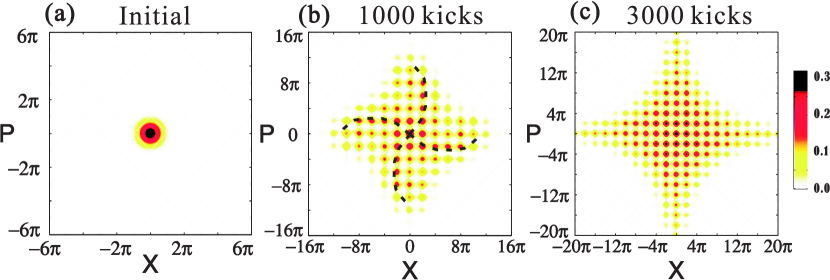
Figure 5: Dissipative quantum dynamics. (a) Husimi $Q$-function of the initial state, which is the ground state of the harmonic trapping potential. (b) Husimi $Q$-function after $1000$ kicks. We mark the main diffusion path by the dashed lines showing a chiral feature. (c) Husimi $Q$-function after $3000$ kicks. In all figures, we set kicking strength $K=0.1$, dissipation rate $\kappa=0.0001$.

In the above section, our analysis is based on the rotating wave approximation where the kicking strength needs to be weak $|K|\ll 1$. In this section, we will investigate the full quantum dynamics of KHO based on the original full Hamiltonian (3) and confirm the validity of the rotating wave approximation, which is used to derive the effective Hamiltonian (8). From a practical point of view, the oscillators are inevitably in contact with the environment, which is conventionally modeled by a harmonic bath model. The coupling with the environment results in dissipation or decoherence of the quantum system. Here, we describe the dissipative dynamics of the quantum KHO by the following master equation,

$$\frac{d{\rho}}{dt}=-\frac{i}{\lambda}[H_{s}(t),\rho]+\kappa(n_{0}+1)\mathcal{D}[\hat{a}]{\rho}+\kappa n_{0}\mathcal{D}[\hat{a}^{\dagger}]{\rho},$$ (16)

where $\kappa$ characterizes the dissipation rate and $n_{0}$ is the Bose-Einstein distribution of the thermal bath. The dissipative dynamics is described by the Lindblad superoperator defined by $\mathcal{D}[\hat{O}]\rho\equiv\hat{O}\rho\hat{O}^{\dagger}-\frac{1}{2}(\hat{O}^{\dagger}\hat{O}\rho+\rho\hat{O}^{\dagger}\hat{O})$, where $\hat{O}$ is an arbitrary operator. The two Lindblad terms in Eq. (16) represents relaxation and heating processes respectively. We notice that some authors also choose the non-Lindblad Caldeira-Leggett master equation to describe the dissipative dynamics Reynoso et al. (2017). Here, we choose the Lindblad master equation (16) since it can give the correct thermal equilibrium state of harmonic oscillator without kicking force while the non-Lindblad Caldeira-Leggett master equation cannot Ramazanoglu (2009).

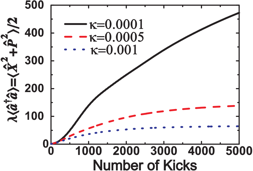
Figure 6: The average energy versus kick number. The averaged energy $\lambda\langle\hat{a}^{\dagger}\hat{a}\rangle=\langle\hat{X}^{2}+\hat{P}^{2}\rangle/2$ is proportional to the area of the lattice size shown in Fig. 5. The black solid line, red dashed line and blue dotted line correspond to the dissipation rate $\kappa=0.0001$, $\kappa=0.0005$ and $\kappa=0.001$ respectively. The kicking strength is $K=0.1$.

As the kicks act as delta-functions, we can separate the dissipative dynamics from the kicking dynamics. In order to solve the dissipative dynamics, we define the characteristic function of the Wigner distribution by Gerry and Knight (2004) $w(s,k)\equiv\int dx\,e^{ixk/\lambda}\langle x+\frac{s}{2}|\rho|x-\frac{s}{2}\rangle,$ Then the master equation (16) without kicking can be transformed into the following Fokker-Planck equation Reynoso et al. (2017)

$$\partial_{t}w+(\frac{\kappa}{2}-\lambda k)\partial_{s}w+(\frac{\kappa}{2}+\lambda s)\partial_{k}w=-\frac{\kappa}{2\lambda}(n_{0}+\frac{1}{2})(s^{2}+k^{2})w.$$ (17)

The dissipative dynamics between two successive kicks is solvable from the above Fokker-Planck equation. Given the initial state at the moment right after $n-1$ kicks $w(s,k;\tau_{n-1}^{+})$, where $\tau_{n-1}^{+}=(n-1)\tau+\Delta$ with a positive infinitesimal increment $\Delta$, the final state at the moment right before $n$ kicks $w(s,k;\tau_{n}^{-})$ with $\tau_{n}^{-}=n\tau-\Delta$, is given by the following map Reynoso et al. (2017)

$$w(s,k;\tau_{n}^{-})=e^{-\frac{n_{0}+1/2}{2\lambda}(1-e^{-\kappa\tau})(s^{2}+k^{2})}w(s_{r},k_{r};\tau_{n-1}^{+})$$ (18)

with $s_{r}=e^{-\frac{\kappa\tau}{2}}(k\sin\tau+s\cos\tau)$ and $k_{r}=e^{-\frac{\kappa\tau}{2}}(k\cos\tau-s\sin\tau)$. The kicking dynamics is an instantaneous unitary transformation $\rho\rightarrow{\rho^{\prime}}=\hat{U}_{K}\rho\hat{U}_{K}^{\dagger}$ with $\hat{U}_{K}\equiv e^{-iK\tau/\lambda\cos\hat{X}}$. In Appendix E, we prove that the corresponding map of the characteristic function of the Wigner distribution at the time $\tau_{n}=n\tau$ is given by

$$w(s,k;\tau_{n}^{+})=\sum_{j=-\infty}^{\infty}J_{j}(2K\sin\frac{s}{2})w(s,k+j\lambda;\tau_{n}^{-}),$$ (19)

where the $J_{j}$ are the $j$th-order cylindrical Bessel function. Hence, the full dynamics of the quantum KHO in contact with a thermal bath is realized by applying the two maps (18) and (19) sequentially. From the characteristic function $w(s,k)$, it is direct to obtain the corresponding Husimi-$Q$ function (see Appendix F).

In Fig. 5(a), we evolve the dynamics of the system starting from the ground state of the harmonic oscillator. We then plot the Husimi $Q$-functions of the states after $1000$ and $3000$ kicks in Fig. 5(b) and Fig. 5(c) respectively. We see clearly that a final state with square lattice structure in phase space forms gradually revealing the underlying square structure of Hamiltonian (8). Interestingly, we find that the transient state shown in Fig. 5(b) has no reflection symmetries with respect to $X$ and $P$ although the RWA Hamiltonian (8) has. There is a chiral feature as marked by the dashed lines along the backbone of the quasiprobability distribution. This chirality is a reflection of the topological property of our system and the noncommutative geometry Connes (1994); Bellissard et al. (1994) of the phase space. As approaching the stationary state, the chirality disappears in the end.

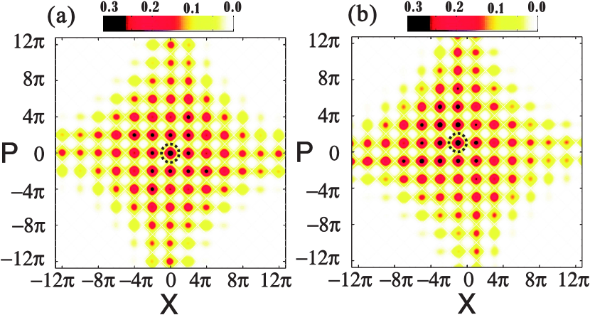
Figure 7: Husimi $Q$-functions for different initial states. The initial state is a coherent state with its center locating on $(0,0)$ and $(-\pi,\pi)$ as marked by two dashed circles in figures (a) and (b) respectively. The $Q$-functions are plotted after $3000$ kicks. Other parameters: $K=0.1$, $\kappa=0.0001$.

Without dissipation, the quantum KHO will experience unbounded diffusion for resonant condition, where the average energy of the harmonic oscillator increases infinitely due to the energy pump from kicking Billam and Gardiner (2009). When dissipation is present, the diffusion process approaches a nonequilibrium stationary state with a finite size in phase space depending on the driving strength and dissipation rate. In Fig. 6, we plot the average energy of the KHO $\lambda\langle\hat{a}^{\dagger}\hat{a}\rangle=\langle\hat{X}^{2}+\hat{P}^{2}\rangle/2$ as a function of the kicking number for different dissipation rates. We see that the smaller the dissipation rate is, the lager the phase space lattice is in the long-time limit. If the dissipation rate is so strong that the system can relax to its ground state during the successive kicks, the lattice state cannot be formed in phase space. Therefore, in order to create a phase space lattice with enough large size, the dissipation rate has to be much weaker than the kicking strength, i.e., $\kappa\ll|K|$.

In Figs. 2(a) and (b), we also notice that there are actually two identical square lattices with a relative shift in phase space, which support eigenstates with positive and negative quasienergy respectively. In Figs. 7(a) and (b), we plot the two Husimi $Q$-functions evolving from two coherent states with different initial positions in phase space, i.e., $(X,P)=(0,0)$ and $(X,P)=(-\pi,\pi)$ respectively. We see that a state initially prepared on one sublattice stays on that lattice during the evolution and has negligible occupation on the other sublattice. This is different from the static potential, where the minimum points correspond to stable state while maximum points correspond to unstable state. Since we are working on a dynamical system far from equilibrium, both minimum and maximum points of the Hamiltonian in phase space are stable; only the saddle points are unstable. This is the reason why we define the Chern number of the gaps symmetrically with respect to the zero line for the Hofstadter’s spectrum in Fig. 3(a).

IV Many-body Dynamics

In the above discussion, we have neglected the interaction terms in the original Hamiltonian (2). From this section, we will consider the interactions between particles. Using the free time-evolution operator $\hat{O}(t)=\exp(i\lambda\sum_{i}\hat{a}_{i}^{\dagger}\hat{a}_{i}t)$ defined at the beginning in Sec. III, the total Hamiltonian in the rotating frame is given by the canonical transformation, i.e., $\hat{O}(t)H(t)\hat{O}^{\dagger}(t)-iO(t)\dot{O}^{\dagger}(t)$. In the RWA, we drop the fast oscillating terms and arrive at the time-independent Hamiltonian

$$H_{RWA}^{T} = \sum_{i}H_{RWA}(\hat{X}_{i},\hat{P}_{i})+\ \sum_{i<j}U(\hat{X}_{i},\hat{P}_{i};\hat{X}_{j},\hat{P}_{j}).$$ (20)

Here, $H_{RWA}(\hat{X}_{i},\hat{P}_{i})$ is the single-particle RWA Hamiltonian given by Eq. (7). The RWA interaction potential $U(\hat{X}_{i},\hat{P}_{i};\hat{X}_{j},\hat{P}_{j})$ is the time-independent part of transformed real space interaction potential $\hat{O}(t)V(\hat{x}_{i}-\hat{x}_{j})\hat{O}^{\dagger}(t)$. In general, $U(\hat{X}_{i},\hat{P}_{i};\hat{X}_{j},\hat{P}_{j})$ is defined in phase space and depends on both coordinates and momenta of two particles. Thus, we call $U(\hat{X}_{i},\hat{P}_{i};\hat{X}_{j},\hat{P}_{j})$ the phase space interaction potential. We aim to determine the explicit form of $U(\hat{X}_{i},\hat{P}_{i};\hat{X}_{j},\hat{P}_{j})$ in this section.

IV.1 Phase Space Interaction Potential

For two arbitrary particles, we introduce the operators $\hat{X}_{c}\equiv(\hat{X}_{1}+\hat{X}_{2})/2,\ \hat{P}_{c}\equiv(\hat{P}_{1}+\hat{P}_{2})/2$ representing the coordinator and momentum of two particles’ center of mass, and the operators $\Delta\hat{X}\equiv\hat{X}_{1}-\hat{X}_{2}$, $\Delta\hat{P}\equiv\hat{P}_{1}-\hat{P}_{2}$ representing their relative displacement in phase space. We further define the operator of phase space distance by

$$\hat{R}\equiv\sqrt{\Delta\hat{X}^{2}+\Delta\hat{P}^{2}}.$$ (21)

It is important to notice that the background of the phase space interaction potential is a noncommutative space. From the commutation relationship $[\hat{X}_{i},\hat{P}_{j}]=i\lambda\delta_{ij}$, we have $[\Delta\hat{X},\Delta\hat{P}]=i(2\lambda)$, and $[\hat{R}^{2},\hat{X}_{c}]=0$ which means the motion of two particles’ center of mass and their relative motion are independent. Thus, we write the common eigenstate of commutative operators $\hat{R}^{2}$ and $\hat{X}_{c}$ as a product state $\Psi(X_{1},X_{2})=f(X_{c})\Phi(X_{1}-X_{2}),$ where the wave function $f(X_{c})$ is the state of two particles’ center of mass and the wave function $\Phi(X_{1}-X_{2})$ describes their relative motion. Reminiscent of the Hamiltonian operator of a harmonic oscillator, the eigenvalues of operator $\hat{R}^{2}$ are given by $4\lambda(N+1/2)$ with $N=0,1,2,\cdot\cdot\cdot$. Therefore, the eigenvalues of the operator $\hat{R}$ are given by

$$R_{N}=2\sqrt{\lambda(N+\frac{1}{2})},\ \ \ N=0,1,2,\cdot\cdot\cdot.$$ (22)

For each $N$, the corresponding eigenstate is given by

$$\Phi_{N}(\Delta X)=\Big{(}\frac{1}{\sqrt{2\lambda\pi}2^{N}N!}\Big{)}^{\frac{1}{2}}H_{N}\Big{(}\sqrt{\frac{1}{2\lambda}}\Delta X\Big{)}e^{-\frac{1}{4\lambda}\Delta X^{2}},$$ (23)

where $H_{N}(\bullet)$ is the Hermite polynomial of degree $N$. We choose functions $\delta(X_{c}-C)$, i.e., the eigenstate of operator $\hat{X}_{c}$, as the basis of two particles’ center of mass. Therefore, we use the Dirac notation $|N,C\rangle$ to represent the total eigenstate, which is determined by two good quantum numbers $C$ and $R_{N}$, i.e., $\hat{X}_{c}|N,C\rangle=C|N,C\rangle$ and $\hat{R}|N,C\rangle=R_{N}|N,C\rangle$. In the coordinate representation, the total eigenstate has the explicit form $\langle X_{1},X_{2}|N,C\rangle=\Psi_{N,C}(X_{1},X_{2})=\delta(X_{c}-C)\Phi_{N}(\Delta X)$.

There is a fundamental difference between the commutative real space and the noncommutative phase space. The concept of point is meaningless in noncommutative space. Instead, we are only allowed to define the coherent state $|\alpha\rangle$ as the point in noncommutative geometry. Similarly, the concept of distance also needs to be reexamined. The distance of two particles in real space is a continuous variable from zero to infinity. However, the distance in phase space is a quantized variable and has a lower limit $\sqrt{2\lambda}$ as seen from Eq. (22). Here, we actually provide a description for the quantization of the noncommutative background.

We now start to determine the phase space interaction potential $U(\hat{X}_{1},\hat{P}_{1};\hat{X}_{2},\hat{P}_{2})$. From the transformation (6), the relative displacement of two particles in the rotating frame is $\hat{O}(t)(\hat{x}_{1}-\hat{x}_{2})\hat{O}^{\dagger}(t)=\Delta\hat{P}\sin t+\Delta\hat{X}\cos t.$ Therefore, for a given real space interaction potential, we have $\hat{O}V(\hat{x}_{1}-\hat{x}_{2})\hat{O}^{\dagger}=\int_{-\infty}^{+\infty}dqV_{q}\hat{Q}$ with the Fourier coefficients $V_{q}=\frac{1}{2\pi}\int_{-\infty}^{+\infty}dxV(x)e^{-iqx}$ and the operator $\hat{Q}\equiv\exp\Big{[}iq(\Delta\hat{P}\sin t+\Delta\hat{X}\cos t)\Big{]}.$ The matrix element of the operator $\hat{Q}$ in the $\hat{R}$-representation is given by the Laguerre polynomials Wüsnche (1991); Guo and Marthaler (2016)

$$\langle N|\hat{Q}|M\rangle=e^{-\frac{\lambda q^{2}}{2}+i(M-N)(\frac{\pi}{2}-\frac{\Omega}{k}t)}\sqrt{\frac{N!}{M!}}\ (\lambda q^{2})^{\frac{M-N}{2}}L_{N}^{M-N}(\lambda q^{2}),\ \ \ \ \ \$$ (24)

where $|N\rangle$ and $|M\rangle$ are the eigenstates of the operator $\hat{R}$ given by Eq. (23). In the RWA, we only keep the time-independent diagonal elements of the matrix (24), i.e., $\langle N|\hat{Q}|N\rangle$ with $N=0,1,2,\cdot\cdot\cdot$. Thus, given an arbitrary real space interaction potential $V(x_{1}-x_{2})$, we find a compact expression for the phase space interaction potential

$$U(\hat{R})=\int_{-\infty}^{+\infty}dqV_{q}e^{-\frac{\lambda q^{2}}{2}}L_{\frac{1}{4\lambda}\hat{R}^{2}-\frac{1}{2}}(\lambda q^{2}).$$ (25)

In the eigenbasis $|N,C\rangle$, we have

$$U(\hat{R})=\sum_{N}U(R_{N})\int dC|N,C\rangle\langle N,C|.$$

Here, the interaction potential $U(\hat{R})$ takes the value $U(R_{N})$ with $R_{N}=2\sqrt{\lambda(N+1/2)}$.

If the two paricles have spins, their spatial state is either antisymmetric or symmetric depending on the symmetry of total spin state, i.e.,

$$\psi_{\pm}(X_{1},X_{2})=\frac{1}{\sqrt{2}}\Big{[}\varphi(X_{1})\phi(X_{2})\pm\phi(X_{1})\varphi(X_{2})\Big{]}.$$

We sperate the average phase space interaction potential by $\langle U\rangle_{\pm}=\langle\psi_{\pm}(X_{1},X_{2})|U(\hat{R})|\psi_{\pm}(X_{1},X_{2})\rangle\equiv U_{c}\pm U_{e}.$ Here, we have defined the direct interaction $U_{c}$ and the the exchange interaction $U_{e}$, respectively,

$$\left\{\begin{array}[]{lll}U_{c}&\equiv&\langle\varphi(X_{1})\phi(X_{2})|U(\hat{R})|\varphi(X_{1})\phi(X_{2})\rangle\\ U_{e}&\equiv&\langle\varphi(X_{1})\phi(X_{2})|U(\hat{R})|\phi(X_{1})\varphi(X_{2})\rangle.\\ \end{array}\right.$$ (28)

The direct interaction part $U_{c}=\frac{1}{2}(\langle U\rangle_{+}+\langle U\rangle_{-})$ corresponds to the classical interaction while the exchange interaction part $U_{e}=\frac{1}{2}(\langle U\rangle_{+}-\langle U\rangle_{-})$ is a pure quantum effect without classical counterpart, which we call $U_{e}$ the Floquet exchange interaction for our system. In the $\hat{R}$-representation, they have been calculated in the Appendix G, i.e.,

$$U_{c}=\sum_{N}U(R_{N})I_{N},\ \ \ \ U_{e}=\sum_{N}(-1)^{N}U(R_{N})I_{N}$$ (29)

with the overlap integral

$$I_{N}=\int dC\Big{|}\langle\varphi(C+\frac{1}{2}\Delta X)\phi(C-\frac{1}{2}\Delta X)|\Phi_{N}(\Delta X)\rangle\Big{|}^{2}.$$ (30)

In the Appendix H, we have given the overlap integral $I_{N}(R)$ for the two displaced coherent states $\varphi(X)=\Big{(}\frac{1}{\sqrt{\pi\lambda}}\Big{)}^{\frac{1}{2}}e^{-\frac{1}{2\lambda}(X-R/2)^{2}}$ and $\phi(X)=\Big{(}\frac{1}{\sqrt{\pi\lambda}}\Big{)}^{\frac{1}{2}}e^{-\frac{1}{2\lambda}(X+R/2)^{2}}$, where $R$ is the distance between the centers of two coherent states in phase space. Below, we will calculate the analytical expressions of $U_{c}(R)$ and $U_{e}(R)$ for contact and hardcore interactions of ultracold atoms.

IV.2 Applications

In this section, we apply our general theory of phase space interaction to the special cases of contact interaction and hardcore interaction for ultracold atoms. We show that, in quasi-1D, the point-like contact interaction in real space becomes a long-range Coulomb-like interaction in phase space. In pure 1D, the hardcore interaction in real space produces a quark-like confinement interaction potential in phase space, which increases linearly with the phase space distance of two atoms.

IV.2.1 Contact Interaction

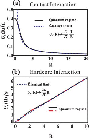
Figure 8: Phase Space Interactions. (a) Contact interaction. The parameter $R$ is the distance between the centers of two coherent states in phase space. The direct phase space interaction potential $U_{c}(R)$ is scaled by the strength of the contact interaction $\varepsilon$. The black solid curve is the result in quantum regime given by Eq. (34) with $\lambda=1$. The blue dashed line is the Coulomb-type interaction (35), which is the result in the classical limit. (b) Hardcore interaction. The direct phase space interaction potential $U_{c}(R)$ is scaled by the radius of hardcore interaction $a$. The black solid curve is the result in quantum regime given by Eq. (39) with $\lambda=1$. The red dotted-dashed line is the result in the linear approximation given by Eq. (40) with $\lambda=1$. The blue dashed line is the linear interaction (41) in the classical limit.

In the experiments, the ultracold atoms are confined in one dimension if the transverse trapping frequency $\omega_{\perp}$ is much larger than the longitudinal trapping frequency $\omega_{z}$. If the characteristic length of transverse trapping $l_{\perp}\equiv\sqrt{\hbar/(m\omega_{\perp})}$ is much larger than the cold atom’s size, i.e., in the quasi-1D, the effective interaction between cold atoms is described by the contact interaction $V(x_{1}-x_{2})=\varepsilon\delta(x_{1}-x_{2})$, where $\varepsilon$ is the interaction strength Bloch et al. (2008); Olshanii (1998); Bergeman et al. (2003). From $V_{q}=\frac{1}{2\pi}\int_{-\infty}^{+\infty}dx\varepsilon\delta(x)e^{-iqx}=\frac{\varepsilon}{2\pi}$ and Eq. (25), the phase space interaction potential can be calculated

$$U(R_{N})=\varepsilon\frac{1+(-1)^{N}}{N\pi\sqrt{2\lambda}}\frac{\Gamma(\frac{N+1}{2})}{\Gamma(\frac{N}{2})}.$$ (31)

Here, $N=0,1,2,3\cdot\cdot\cdot$ and $\Gamma(\bullet)$ is the gamma function. We see that $U(R_{N})$ is zero for odd integer $N$ and finite for even integer $N$. The wave function of two atoms’ relative motion $\Phi_{N}(\Delta X)$ is antisymmetric for odd $N$, which means the probability amplitude is zero when the two atoms contact each other. The result is that the total average interaction of $\Phi_{N}(\Delta X)$ is zero for odd $N$.

The direct phase space interaction $U_{c}(R)$ and Floquet exchange interaction $U_{e}(R)$ of two cold atoms, which are described by two coherent states, can be calculated from Eq.s (29), (31) and (93)

$$\left\{\begin{array}[]{lll}U_{c}(R)=\frac{\varepsilon}{\sqrt{2\pi\lambda}}\exp\Big{(}-\frac{R^{2}}{4\lambda}\Big{)}\ I_{0}\Big{(}\frac{R^{2}}{4\lambda}\Big{)}\\ U_{e}(R)=U_{c}(R).\\ \end{array}\right.$$ (34)

Here, $R$ is the distance in phase space between the centers of two coherent states and $I_{0}(\bullet)$ is the zeroth order modified Bessel function of the first kind. In the large distance limit, we use the asymptotic behavior of the special function $I_{0}(z)\sim e^{z}/\sqrt{2\pi z}$ for $z\gg 1$ and have

$$U_{c}(R) \sim \frac{\varepsilon}{\pi}\frac{1}{R},\ \ \ \ \mathrm{for}\ \ R\gg 2\sqrt{\lambda}.$$ (35)

In Fig. 8(a), we plot the $U_{c}(R)$ as function of $R$ and its long-range asymptotic behavior. We see that a point-like contact interaction indeed becomes a long-range Coulomb-like interaction in the long-distance limit, which is consistent with the pure classical analysis Guo et al. (2016).

As shown in Eq. (34), we also find that the Floquet exchange interaction is equal to the direct phase space interaction, i.e., $U_{e}(R)=U_{c}(R)$, and does not disappear even in the classical limit $\lambda\rightarrow 0$, which cannot happen in a static system. Usually, the effective spin-spin interaction in Heisenberg model comes from the quantum exchange interaction between the nearest-neighbouring electrons and cannot be explained by classical dynamics. One should always keep in mind that we are investigating the effective stroboscopic dynamics and the two atoms indeed collide with each other during every stroboscopic time step. The phase space interaction is actually the time-averaged real space interaction in one harmonic period. The spin-spin interaction in Heisenberg model is a short-range interaction due to the exponentially small wave function overlap of two next-nearest-neighbouring electrons. However, here in our system, the Floquet exchange interaction has long-range behavior following Coulomb’s law. In the classical limit $\lambda\rightarrow 0$, the long-range Floquet exchange interaction can be viewed as an effective long-range spin-spin interaction induced by collision of two atoms. The equality $U_{e}(R)=U_{c}(R)$ comes from the $\delta$ function modelling the contact interaction and the fact that the spatial antisymmetric state of two atoms has zero probability to touch each other. If the interaction potential between cold atoms is different from the $\delta$-function model, it is possible to tune the phase space interaction $U_{c}(R)$ and collision-induced spin-spin interaction $U_{e}(R)$ independently in the experiments.

IV.2.2 Hardcore Interaction

If the characteristic length of transverse trapping $l_{\perp}$ is much smaller than the cold atom’s size, which is called pure-1D, the contact interaction is no longer valid for the description of interaction between cold atoms Astrakharchik et al. (2004); Paredes et al. (2004); Kinoshita et al. (2004); Haller et al. (2009). In this situation, the atom can be viewed as a hardcore particle with a radius $a$, which means the interaction potential between the two atoms is infinite when their distance is smaller than $2a$ and zero when the distance is larger than $2a$. Our theory of phase space interaction can be applied to the small hardcore limit $a\ll\sqrt{\lambda}$. Since the two atoms can not contact each other due to the hardcore interaction, the engenstates of phase space distance operator $\hat{R}$ have to be zero at zero distance, which means that only the odd eigenstates $\Phi_{2m+1}(\Delta X)$ with $m\in\mathbb{N}$ satisfy this condition. The even eigenstate should be reconstructed as $\Phi_{2m}(\Delta X)=\mathrm{sgn}(\Delta X)\Phi_{2m+1}(\Delta X)$ with $\mathrm{sgn}(\bullet)$ the sign function. The eigenstates $\Phi_{2m}(\Delta X)$ and $\Phi_{2m+1}(\Delta X)$ are degenerate with the same eigenvalue $R_{2m}=R_{2m+1}=2\sqrt{\lambda(2m+3/2)}$. In the Appendix I, we calculate the phase space interaction potential of the hardcore interaction potential for odd integers $N=2m+1$

$$U(R_{N}) = \frac{a\sqrt{2\lambda/\pi}}{2^{-N}N!}\sum_{k,l=0}^{[\frac{N}{2}][\frac{N}{2}]}\,\frac{(-1)^{k+l}(N!)^{2}(N-k-l)!}{2^{2k+2l}k!l!(N-2k)!(N-2l)!}$$ (36)

$$\approx \frac{2a}{\pi}R_{N}.\ \ \ \ \$$

Here, $[\frac{N}{2}]$ means the closest integer number less than $\frac{N}{2}$. For even integers $N=2m$, we have $U(R_{2m})=U(R_{2m+1})$. Here, we find that $U(R_{N})$ can be approximated very well by the linear relationship $U(R_{N})\approx 2a\pi^{-1}R_{N}$.

The direct phase space interaction $U_{c}(R)$ and the Floquet exchange interaction $U_{e}(R)$ of two coherent states can be calculated from Eq.s (29), (36)

$$\left\{\begin{array}[]{lll}U_{c}(R)=2\sum_{m=0}U(R_{2m+1})I_{2m+1}\\ U_{e}(R)=0.\\ \end{array}\right.$$ (39)

Here, $R$ is phase space distance between the centers of two coherent states and the overlap integral $I_{2m+1}$ is given by Eq. (93). The zero Floquet exchange interaction comes from the degeneracy of the symmetric and antisymmetric states. Thus, there is no collision-induced spin-spin interaction for the hardcore interaction. Using the linear approximation $U(R_{N})\approx 2a\pi^{-1}R_{N}$ and Eq. (39), we have

$$U_{c}(R) \approx \frac{8a\sqrt{\lambda}}{\pi}\sum_{m=0}^{\infty}\,\frac{\sqrt{2m+3/2}}{(2m+1)!}\,\exp\Big{(}-\frac{R^{2}}{4\lambda}\Big{)}\Big{(}\frac{R^{2}}{4\lambda}\Big{)}^{2m+1}.\ \ \$$ (40)

In the long-distance limit, we have the asymptotic expression of Eq. (40), i.e.,

$$U_{c}(R)\rightarrow\frac{2a}{\pi}R,\ \ \ \ \mathrm{for}\ \ R\gg 2\sqrt{\lambda}.$$ (41)

This is consistent again with the classical analysis Guo et al. (2016). In Fig. 8(b), we plot the direct phase space interaction potential $U_{c}(R)$ as a functions of phase space distance $R$. We see that the linear relationship (41) (blue dashed line) is a very good approximation of Eq. (39) (black solid curve) and Eq. (40) (red dotted-dashed curve). It is interesting to find that the linear phase space interaction potential (41) mimics the interaction potential between quarks in QCD Trawiński et al. (2014); Jido and Sakashita (2016). Actually, this surprising behavior of hardcore atoms can be understood in a simple picture. Since the two atoms have a tiny hardcore radius $a$, they prefer to oscillate in a synchronized way, i.e., in phase. If the atoms are out of phase due to the finite phase space distance $R$, they are more likely to collide with each other during the oscillation. The collision effect becomes stronger as the phase space distance $R$ is larger, resulting in a confinement potential in the end.

IV.3 Classical Many-body Dynamics

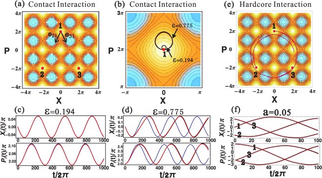
Figure 9: Classical Three-body Dynamics. (a) The initial conditions of three atoms (red dots). (b) Phase space trajectories of the first atom with different contact interaction strengths $\varepsilon=0.194$ (small circle) and $\varepsilon=0.775$ (large circle). (c) Time evolutions of the first atom’s position and momentum with contact interaction strength $\varepsilon=0.194$. (d) Time evolutions of the first atom’s position and momentum with contact interaction strength $\varepsilon=0.775$. (e) Phase space trajectories of three atoms with hardcore interaction strength $a=0.05$. (f) Time evolutions of all the three atoms’ positions and momenta with hardcore interaction strength $a=0.05$. In all figures, the black dots are the results obtained from Poincaré map and the red lines are the results calculated from the RWA EOM (46). In (b), (c) and (d), the blue lines are the results given by the linear solution (47) and the black dots are so dense that they look like lines. Other parameters: kicking strength $K=-0.02\pi^{-1}$.

Although it is very difficult to numerically simulate the quantum many-body dynamics from the original many-body Hamiltonian (2), we can simulate the classical many-body dynamics and verify our theory of phase space interaction. From now on, we consider the classical dynamics of spinless atoms and replace all the operators by their corresponding classical quantities. The time evolution of the original coordinates, $x_{i}(t)$ and $p_{i}(t)$, of a single atom are given by the canonical equations of motion (EOM) from Eq. (2)

$$\frac{dx_{i}}{dt}=\frac{\partial H(t)}{\partial p_{i}},\ \ \ \ \ \frac{dp_{i}}{dt}=-\frac{\partial H(t)}{\partial x_{i}}.$$ (42)

As seen from Eq. (6), the values of $X_{i}(t)$ and $P_{i}(t)$ can be obtained from the time evolution of $x_{i}(t)$ and $p_{i}(t)$ stroboscopically every time period of $2\pi$. In this sense, the $X_{i}(t)$ and $P_{i}(t)$ define the time evolution of the amplitude and phase of an oscillating atom in the discrete time domain $t=2\pi m$ with $m=0,1,2,\cdot\cdot\cdot$. This method is called $Poincar\acute{e}\ map$ Rasband ; Devaney (2003).

In the rotating frame, we write the RWA many-body Hamiltonian explicitly for $q_{0}=4$

$$H_{RWA}^{T} = \sum_{i}\frac{K}{2}\Big{(}\cos X_{i}+\cos P_{i}\Big{)}+\sum_{i<j}U_{c}(R_{ij}),$$ (43)

where $R_{ij}=\sqrt{(X_{i}-X_{j})^{2}+(P_{i}-P_{j})^{2}}$ is the classical phase space distance of two arbitrary atoms. Depending on the original interaction potential, the phase space interaction potential $U_{c}(R_{ij})$ takes the form of either Eq. (35) or Eq. (41). The EOM of $X_{i}(t)$ and $P_{i}(t)$ is described by ${dX_{i}}/{dt}={\partial H_{RWA}^{T}}/{\partial P_{i}},\ {dP_{i}}/{dt}=-{\partial H_{RWA}^{T}}/{\partial X_{i}}.$ Using Eq. (43), we have the explicit form of EOM

$$\left\{\begin{array}[]{lll}\frac{d}{dt}X_{i}&=&-\frac{1}{2}K\sin P_{i}+\sum_{j}\frac{dU_{c}(R_{ij})}{dR_{ij}}\frac{P_{i}-P_{j}}{R_{ij}}\\ \frac{d}{dt}P_{i}&=&\ \ \frac{1}{2}K\sin X_{i}-\sum_{j}\frac{dU_{c}(R_{ij})}{dR_{ij}}\frac{X_{i}-X_{j}}{R_{ij}}.\end{array}\right.$$ (46)

Using the above two methods, we can calculate the dynamics of many interacting atoms, and compare them to verify our phase space interaction theory.

In Fig. 9, we investigate the dynamics of three interacting particles. For convenience, we introduce the complex position of the $j$th atom in phase space $\mathbf{Z}_{j}(t)\equiv X_{j}(t)+iP_{j}(t)$. As shown in Fig. 9(a), we set the three atoms initially at the local equilibrium points of single particle Hamiltonian, i.e., $\mathbf{Z}_{1}(0)=2\pi i$, $\mathbf{Z}_{2}(0)=-2\pi-2\pi i$ and $\mathbf{Z}_{3}(0)=2\pi-2\pi i$. If the displacement of each atom in phase space is small, i.e., $|\mathbf{Z}_{i}(t)-\mathbf{Z}_{i}(0)|\ll 1$, we can linearize the EOM (46), and have the following solution

$$\mathbf{Z}_{i}(t)\approx\mathbf{Z}_{i}(0)+\frac{2}{K}\Big{(}e^{i\frac{1}{2}Kt}-1\Big{)}\sum_{j\neq i}\frac{dU_{c}}{dR_{ij}}\mathbf{e}_{ji},$$ (47)

where $\mathbf{e}_{ji}\equiv[\mathbf{Z}_{j}(0)-\mathbf{Z}_{i}(0)]/|\mathbf{Z}_{j}(0)-\mathbf{Z}_{i}(0)|$ is the unit vector directing from $i$th atom’s initial position to $j$th atom’s initial position in phase space as shown by the black arrows in Fig. 9(a). The above linear solution indicates that each atom oscillates harmonically around a shifted equilibrium point $\mathbf{Z}_{i}(0)-2K^{-1}\sum_{j\neq i}({dU_{c}}/{dR_{ij}})\mathbf{e}_{ji}$ and with the amplitude $\Delta\mathbf{Z}_{i}=2K^{-1}|\sum_{j\neq i}({dU_{c}}/{dR_{ij}})\mathbf{e}_{ji}|$.

In Figs. 9(b)-(d), we show the three-body dynamics with the real space contact interaction potential $V(x_{i}-x_{j})=\varepsilon\delta(x_{i}-x_{j})$, which is modeled by a Lorentz function $V(x_{i}-x_{j})=\frac{\varepsilon}{\pi}\frac{\sigma}{(x_{i}-x_{j})^{2}+\sigma^{2}}$ with $\sigma=0.1$ in our numerical simulations. The corresponding phase space interaction potential is given by $U_{c}(R_{ij})=\frac{\varepsilon}{\pi}\frac{1}{R_{ij}}$. We plot the phase space trajectories of the first atom for different interaction strengths $\varepsilon=0.194$ and $\varepsilon=0.775$ in Fig. 9(b), and the corresponding time evolutions of positions and momenta in Figs. 9(c) and (d). We see that the dynamics given by the three methods agree with each other very well for weak interaction $\varepsilon=0.194$ as shown in Fig. 9(c). However, for a larger interaction $\varepsilon=0.775$, the linear solution (47) breaks down while the RWA EOM (46) is still a very good approximation as shown in Fig. 9(d).

In Figs. 9(e) and (f), we show the three-body dynamics with the hardcore interaction, which is modeled approximately by an inverse power-law potential $V(x_{i}-x_{j})=\frac{(2a)^{n}}{(x_{i}-x_{j})^{n}}$ with a high power $n=20$ in our numerical simulations. The corresponding phase space interaction potential is given by $U_{c}(R_{ij})=2a\pi^{-1}R_{ij}$. As shown in Fig. 9(e), for a small hardcore radius $a=0.05$, the phase space interaction is already strong enough to make the three particles overcome the potential barrier of phase space lattice and exhibit global motions. In Fig. 9(f), we compare the results from Poincar$\acute{e}$ map (black dots) and the RWA EOM (46) (red lines), which agree with each other very well.

IV.4 Dynamical Crystals

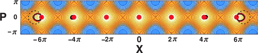
Figure 10: One-dimensional Dynamical Crystal. The initial positions of seven atoms are marked by red dots. Black lines and red lines are the phase space trajectories calculated from Poincaré map and RWA EOM (46) with contact interaction strength $\varepsilon=0.194$. The one-dimensional dynamical crystal survives if the two atoms at the ends oscillate inside the dashed circles. Kicking strength: $K=-0.02\pi^{-1}$.

In Fig. 10, we show the dynamics of seven interacting atoms for contact interaction with $\varepsilon=0.194$. The seven atoms are located initially at the equilibrium points with zero momenta as shown by the seven red dots. It can be seen that the two atoms at the ends oscillate with the largest amplitude. If the interaction is weak enough, the atoms only oscillate locally around their equilibrium points. If the interaction is strong enough, the two edge atoms can overcome the potential barrier of the phase space lattice, and destroy the crystal state. The existence of the crystal state is guaranteed by the condition that the oscillating amplitude of the edge atom $\Delta\mathbf{Z}_{\mathrm{edge}}$ is smaller than the radius of the dashed circle indicated in Fig. 10, i.e., $\Delta\mathbf{Z}_{\mathrm{edge}}<(\sqrt{2}-1)\pi$. We can estimate the critical condition from the linear solution (47). For the contact interaction, the oscillating amplitude of the edge atom converges for infinite atoms, i.e., $\Delta\mathbf{Z}_{\mathrm{edge}}=\frac{\varepsilon}{12\pi K}$. Therefore, the critical interaction strength for the existence of 1D crystal state in phase space is given by

$$\varepsilon_{c}\approx 12(\sqrt{2}-1)\pi^{2}K.$$ (48)

For hardcore interaction with $U_{c}(R_{ij})=2a\pi^{-1}R_{ij}$, the oscillating amplitudes of the two edge atoms can be estimated by $\Delta\mathbf{Z}_{\mathrm{edge}}=\frac{4a}{\pi K}(N-1)$, where $N$ is the number of atoms. The oscillating amplitude $\Delta\mathbf{Z}_{\mathrm{edge}}$ increases linearly with the number of atoms, which means it is impossible to create an infinitely long 1D crystal state with hardcore interaction. For a given kicking strength $K$ and hardcore radius $a$, the critical atom number for the existence of 1D crystal state is

$$N_{c}\approx(\sqrt{2}-1)\pi^{2}\frac{K}{4a}.$$ (49)

We call the stable crystal state in phase space formed by many atoms, the dynamical crystals.

One should distinguish the concepts of phase space lattice discussed in Sec. III and the dynamical crystal introduced here. Phase space lattice refers to the periodic structure in phase space of the single-particle Hamiltonian (7) without consideration of atomic interaction, while the dynamical crystal refers to the many-body state formed by interacting atoms. In the experiments, the dynamical crystal can be realized by two basic steps: first, prepare the initial state of atoms via applying a very strong static optical lattice; then, suddenly turn off the strong static optical lattice and add a weak optical lattice stroboscopically.

If the atoms have spins and tightly bound at the their fixed points by the phase space lattice, the direct phase space interaction $U_{c}(R)$ does not play a role in the dynamics. However, as discussed in Sec. IV.2.1, the contact interaction can induce a Coulomb-like Floquet exchange interaction $U_{e}(R)=\frac{\varepsilon}{\pi}\frac{1}{R}$, and thus the system shown in Fig. 10 can be modelled by a 1D spin chains with isotropic spin-spin interaction. The famous Mermin-Wagner theorem claims that, at any nonzero temperature, a one- or two-dimensional isotropic Heisenberg model with finite-range exchange interaction can be neither ferromagnetic nor antiferromagnetic Mermin and Wagner (1966). This theorem clearly excludes a variety of types of long-range ordering in low dimensions, and is crucial to the search for low-dimensional magnetic materials in the recent years Gong et al. (2017); Huang et al. (2017); Blanchard et al. (2013). Here in our model, the collision-induced spin-spin interaction has a Coulomb-like long-range behavior, which is beyond the definition of finite-range interaction in Mermin-Wagner theorem sho . Hence, the dynamical crystals actually provide a possible platform to test the Mermin-Wagner theorem and search for other new phenomena with long-range interactions such as causality and quantum criticality Hauke and Tagliacozzo (2013); Richerme et al. (2014); Gong et al. (2014); Métivier et al. (2014); Foss-Feig et al. (2015); Maghrebi et al. (2016); Buyskikh et al. (2016), nonlocal order Torre et al. (2006); Berg et al. (2008); Endres et al. (2011), etc.

V Summary

In summary, we have studied the possibility to create new physics by Floquet many-body engineering in the dynamical system of kicked interacting particles in 1D harmonic potential. Our system exhibits surprisingly rich topological and many-body physics in 2D phase space. In the weak kicking strength regime $K\ll 1$, the single-particle RWA Hamiltonian has various lattice structures in phase space depending on the kicking period. The topological physics comes from the noncommutative geometry of phase space, which naturally provides a geometric quantum phase. We analyzed the topological quasienergy band structure of the square phase space lattice. We investigated the full dissipative quantum dynamics of a single kicked harmonic oscillator using master equation and the Fokker-Planck equation. The time evolution of the Husimi $Q$-functions confirms that the nonequilibrium stationary state is indeed a lattice state in phase space, but has a finite size due to the dissipation.

For the many-body dynamics, we made several findings and predictions based on the theory of phase space interaction potential. We found that the original contact interaction becomes a long-range Coulomb-like interaction in phase space, and the hardcore interaction becomes a quark-like confinement interaction in phase space. For the contact interaction, we predicted that the long-range Floquet exchange interaction does not disappear even in the classical limit, and can be viewed as collision-induced spin-spin interaction. We investigated the classical many-body dynamics and proposed the concept of dynamical crystals. We found that the contact interaction can create an infinitely long 1D dynamical crystal but the hardcore interaction cannot.

Finally, we point out that our method can increase the speed of numerical simulation significantly. For example, in simulating the dynamics of seven interacting atoms in Sec. IV.4, the method of Poincaré map based on the original Hamiltonian costs more than ten hours using Wolfram Mathematica while the method based on the phase space interaction only needs one second. The reason is that our method only needs to calculate the dynamics on the stroboscopic time points by averaging the dynamics between stroboscopic steps using the phase space interaction potential.

Recently, we learned of a related study Giergiel et al. (2017) in which the authors also discussed that the contact interactions between atoms can result in exotic long-range interactions in the effective description of the resonantly driven many-body system.

Acknowledgements

LG and PL acknowledge financial support from Carl-Zeiss Stiftung (0563-2.8/508/2).

Appendix A RWA Floquet Hamiltonian

The method we adopt here is the same as that in Guo and Marthaler (2016). We start with the dimensionless Hamiltonian (3). To be clear, we write it again here

$$H_{s}=\frac{1}{2}(\hat{x}^{2}+\hat{p}^{2})+K\tau\cos\hat{x}\sum_{n}\,\delta(t-n\tau),$$ (50)

where we have neglected the particle index and simplified the notation of the summation in the kicking part. As discussed in the main text, we transform Eq. (50) into the rotating frame by employing the unitary transformation $\hat{O}=\exp\big{[}i(\hat{a}^{\dagger}\hat{a}+1/2)t\big{]}$ and using the relationship (6)

$$H_{RF} = \hat{O}H_{s}\hat{O}^{\dagger}-i\lambda\hat{O}\dot{\hat{O}}^{\dagger}$$

$$= K\hat{O}\cos\hat{x}\,\hat{O}^{\dagger}\sum_{n}\,\delta(\frac{t}{\tau}-n)$$

$$= \frac{K}{2}\Big{[}\hat{M}(\hat{X},\hat{P})+\hat{M}^{\dagger}(\hat{X},\hat{P})\Big{]}\sum_{n}\,\delta(\frac{t}{\tau}-n),$$

where we define $\hat{M}(\hat{X},\hat{P})=\exp\Big{\{}i\big{[}\hat{X}\cos t+\hat{P}\sin t\big{]}\Big{\}}$. The harmonic term in Eq. (A) disappears due to the resonant condition.

The element of $\hat{M}(\hat{X},\hat{P})$ in the basis of Fock states is evaluated to be Wüsnche (1991); Guo and Marthaler (2016)

$$\langle l|\hat{M}(\hat{X},\hat{P})|k\rangle = e^{-\lambda/4+i(k-l)(\pi/2-t)}\sqrt{\frac{l!}{k!}}\left(\frac{\lambda}{2}\right)^{\frac{k-l}{2}}$$ (52)

$$\times L^{k-l}_{l}(\lambda/2).$$

Here the $L_{l}^{k-l}$ are the generalized Laguerre polynomials. Inserting Eq. (52) into $\hat{H}_{RF}$ we have

$$H_{RF} = \frac{K}{2}\bigg{[}\sum_{k,l}\,e^{-\lambda/4+i(k-l)(\pi/2-t)}\sqrt{\frac{l!}{k!}}\left(\frac{\lambda}{2}\right)^{\frac{k-l}{2}}$$ (53)

$$\times L^{k-l}_{l}\left(\lambda/2\right)|l\rangle\langle k|+h.c.\bigg{]}\sum_{n}\,\delta(\frac{t}{\tau}-n).$$

The sum of the Dirac $\delta$-functions in Eq. (53) obeys the following identity Zaslavsky (2008)

$$\sum_{n}\,\delta(\frac{t}{\tau}-n)=\sum_{n}\,\cos\frac{2\pi nt}{\tau}.$$ (54)

Making use of this relation and dropping all terms relevant to $t$ in $\hat{H}_{RF}$ (rotating wave approximation) we get

$$H_{RWA} = \frac{K}{2}\bigg{[}\sum_{l,n}\,e^{-\lambda/4+inq_{0}\pi/2}\sqrt{\frac{l!}{(l+nq_{0})!}}\left(\frac{\lambda}{2}\right)^{\frac{nq_{0}}{2}}$$ (55)

$$\times L_{l}^{nq_{0}}\left(\lambda/2\right)|l\rangle\langle l+nq_{0}|+h.c.\bigg{]}.$$

The sum over $n$ can be formulated as the sum over $k=l+nq_{0}$ with the help of the formula

$$\frac{1}{q_{0}}\sum\limits_{j=1}^{q_{0}}\,e^{-i2\pi(k-l)j/q_{0}}=\begin{cases}0,&(k-l)/q_{0}\not\in\mathbb{Z}\\ 1,&(k-l)/q_{0}\in\mathbb{Z},\end{cases}$$

that is,

$$H_{\it RWA} = \frac{K}{2q_{0}}\bigg{[}\sum_{j=1}^{q_{0}}\sum_{k,l}\,e^{-\lambda/4+i(k-l)(\pi/2-2\pi j/q_{0})}\sqrt{\frac{l!}{k!}}\left(\frac{\lambda}{2}\right)^{\frac{k-l}{2}}$$ (56)

$$\times L^{k-l}_{l}\left(\lambda/2\right)|l\rangle\langle k|+h.c.\bigg{]}.$$

Using Eq. (52), we have the final effective Hamiltonian

$$H_{RWA} = \frac{K}{2q_{0}}\sum_{j=1}^{q_{0}}\bigg{[}e^{i\hat{X}\cos(2\pi j/q_{0})+i\hat{P}\sin(2\pi j/q_{0})}+h.c.\bigg{]}$$ (57)

$$= \frac{K}{q_{0}}\sum_{j=1}^{q_{0}}\,\cos\left(\hat{X}\cos\frac{2\pi j}{q_{0}}+\hat{P}\sin\frac{2\pi j}{q_{0}}\right).$$

Another way to derive the effective Hamiltnoian Eq. (7) is to start from the Floquet operator in one harmonic oscillation

$$\hat{F}^{q_{0}}=\Big{[}e^{-i(\hat{x}^{2}+\hat{p}^{2})\tau/2\lambda}e^{-iK\cos{\hat{x}}/\lambda}\Big{]}^{q_{0}}.$$ (58)

Following the same procedure in Billam and Gardiner (2009) , we can reformulate Eq. (58) as

$$\hat{F}^{q_{0}}=\prod_{j=0}^{q_{0}-1}\exp\Bigg{\{}-iK\cos\Big{[}\sqrt{\frac{\lambda}{2}}(\hat{a}e^{-i2\pi j/q_{0}}+\hat{a}^{\dagger}e^{i2\pi j/q_{0}})\Big{]}/\lambda\Bigg{\}}.$$

Expanding $\hat{F}^{q_{0}}$ into a power series of the kicking strength $K$ and keeping the terms in the first order, we again get the effective Hamiltonian $\hat{H}_{RWA}$.

Appendix B Calculation of $\langle\alpha|H_{\it RWA}(\hat{X},\hat{P})|\alpha\rangle$

Defining displacement operator $D_{\alpha}\equiv e^{\alpha\hat{a}^{\dagger}-\alpha^{*}\hat{a}}$, then we have the following relationship

$$\left\{\begin{array}[]{lll}D_{\alpha}D_{\beta}=e^{i\mathrm{Im}(\alpha\beta^{*})}D_{\alpha+\beta},\\ D_{\alpha}|\beta\rangle=e^{i\mathrm{Im}(\alpha\beta^{*})}|\alpha+\beta\rangle.\\ \end{array}\right.$$ (61)

We consider a general Hamiltonian $H=\cos(p\hat{X}+q\hat{P})$ which can be rewritten as

$$H = \cos(p\hat{X}+q\hat{P})$$ (62)

$$= \frac{1}{2}\Big{(}e^{ip\hat{X}+iq\hat{P}}+e^{-ip\hat{X}-iq\hat{P}}\Big{)}$$

$$= \frac{1}{2}\Big{[}e^{-\sqrt{\frac{\lambda}{2}}(q-ip)\hat{a}^{\dagger}+\sqrt{\frac{\lambda}{2}}(q+ip)\hat{a}}+h.c.\Big{]}$$

$$= \frac{1}{2}\Big{[}D_{-\sqrt{\frac{\lambda}{2}}(q-ip)}+D_{\sqrt{\frac{\lambda}{2}}(q-ip)}\Big{]}.$$

Here we have used $\hat{X}=\sqrt{\frac{\lambda}{2}}(\hat{a}^{\dagger}+\hat{a})$ and $\hat{P}=i\sqrt{\frac{\lambda}{2}}(\hat{a}^{\dagger}-\hat{a})$. Using the relationship (61) and the identity $\langle\alpha|\beta\rangle=e^{-|\alpha|^{2}/2-|\beta|^{2}/2+\alpha^{*}\beta}$, we have the matrix element of Hamiltonian $H=\cos(p\hat{X}+q\hat{P})$ in coherent state representation

$$\langle\alpha|H|\beta\rangle = \frac{1}{2}\Big{(}\Big{\langle}\alpha\Big{|}\beta-\sqrt{\frac{\lambda}{2}}(q-ip)\Big{\rangle}e^{-i\sqrt{\frac{\lambda}{2}}\mathrm{Im}[(q-ip)\beta^{*}]}+\Big{\langle}\alpha\Big{|}\beta+\sqrt{\frac{\lambda}{2}}(q-ip)\Big{\rangle}e^{i\sqrt{\frac{\lambda}{2}}\mathrm{Im}[(q-ip)\beta^{*}]}\Big{)}$$ (63)

$$= \frac{1}{2}\Big{(}e^{-\frac{1}{2}|\alpha|^{2}-\frac{1}{2}|\beta-\sqrt{\frac{\lambda}{2}}(q-ip)|^{2}+\alpha^{*}\beta-\alpha^{*}\sqrt{\frac{\lambda}{2}}(q-ip)-i\sqrt{\frac{\lambda}{2}}\mathrm{Im}[(q-ip)\beta^{*}]}+e^{(-\frac{1}{2}|\alpha|^{2}-\frac{1}{2}|\beta+\sqrt{\frac{\lambda}{2}}(q-ip)|^{2}+\alpha^{*}\beta+\alpha^{*}\sqrt{\frac{\lambda}{2}}(q-ip)+i\sqrt{\frac{\lambda}{2}}\mathrm{Im}[(q-ip)\beta^{*}]}\Big{)}$$

$$= \frac{1}{2}e^{-\frac{1}{2}|\alpha|^{2}-\frac{1}{2}|\beta|^{2}+\alpha^{*}\beta-\frac{\lambda}{4}|q-ip|^{2}}\Big{(}e^{\frac{\beta}{2}\sqrt{\frac{\lambda}{2}}(q+ip)+(\frac{\beta^{*}}{2}-\alpha^{*})\sqrt{\frac{\lambda}{2}}(q-ip)-\frac{1}{2}\sqrt{\frac{\lambda}{2}}[(q-ip)\beta^{*}-(q+ip)\beta]}+e^{-\frac{\beta}{2}\sqrt{\frac{\lambda}{2}}(q+ip)-(\frac{\beta^{*}}{2}-\alpha^{*})\sqrt{\frac{\lambda}{2}}(q-ip)+\frac{1}{2}\sqrt{\frac{\lambda}{2}}[(q-ip)\beta^{*}-(q+ip)\beta]}\Big{)}$$

$$= \frac{1}{2}e^{-\frac{1}{2}|\alpha|^{2}-\frac{1}{2}|\beta|^{2}+\alpha^{*}\beta-\frac{\lambda}{4}|q-ip|^{2}}\Big{(}e^{\beta\sqrt{\frac{\lambda}{2}}(q+ip)-\alpha^{*}\sqrt{\frac{\lambda}{2}}(q-ip)}+e^{-\beta\sqrt{\frac{\lambda}{2}}(q+ip)+\alpha^{*}\sqrt{\frac{\lambda}{2}}(q-ip)}\Big{)}$$

$$= \frac{1}{2}e^{-\frac{1}{2}|\alpha|^{2}-\frac{1}{2}|\beta|^{2}+\alpha^{*}\beta-\frac{\lambda}{4}|q-ip|^{2}}\Big{(}e^{\sqrt{\frac{\lambda}{2}}(\beta-\alpha^{*})q+i\sqrt{\frac{\lambda}{2}}(\beta+\alpha^{*})p}+e^{-\sqrt{\frac{\lambda}{2}}(\beta-\alpha^{*})q-i\sqrt{\frac{\lambda}{2}}(\beta+\alpha^{*})p}\Big{)}.$$

By defining the average coordinator and momentum

$$\left\{\begin{array}[]{lll}X\equiv\langle\alpha|X|\alpha\rangle=\sqrt{\frac{\lambda}{2}}(\alpha^{*}+\alpha)\\ P\equiv\langle\alpha|P|\alpha\rangle=i\sqrt{\frac{\lambda}{2}}(\alpha^{*}-\alpha),\\ \end{array}\right.$$ (66)

we have the diagonal elements of $H=\cos(p\hat{X}+q\hat{P})$

$$\langle\alpha|H|\alpha\rangle=\exp\Big{(}-\frac{\lambda}{4}|q-ip|^{2}\Big{)}\cos(pX+qP).$$ (67)

Using Eq. (67) by setting $p=\cos\frac{2\pi j}{q_{0}}$ and $q=\sin\frac{2\pi j}{q_{0}}$, we can easily obtain $\langle\alpha|H_{\it RWA}(\hat{X},\hat{P})|\alpha\rangle=e^{-\lambda/4}H_{\it RWA}(X,P)$.

Appendix C Zak’s $kq$ Representation

The $kq$ representation introduced in Ref. Zak (1972) is the complete orthonormal basis constructed by the common eigenstates of the translation operators in both $X$ and $P$ directions. In general, for the translation operation in $X$ direction $e^{i\hat{P}A/\lambda}$, the “shortest" commutative translation operator in $P$ direction is $e^{i\hat{X}B/\lambda}$ with $B=2\pi\lambda/A$. Given the dimensionless Planck constant $\lambda=p/q$, where $p$ and $q$ are coprime integers, we choose $A=2\pi/q$ and $B=2\pi p$ for constructing our Zak’s $kq$ representation. In the coordinate representation, the basis for given quantum numbers $k_{X}$ and $k_{P}$ is Zak (1972)

$$\phi_{{(k_{X},k_{P})}}(X)=\sqrt{\frac{\lambda}{q}}\sum_{l}e^{ik_{X}\frac{2\pi l}{q}}\delta(X-\lambda k_{P}-\frac{2\pi l}{q})$$ (68)

with $l\in\mathbb{Z}$. State function (68) is composed of a series of Dirac’s delta function with shifted phases. Note that the quantum numbers $k_{X}$ and $k_{P}$ take value in the region $0\leq k_{X}<q,0\leq k_{P}<1/p$, which is $q$-times larger than the Brillioun zone. Since function (68) is the eigenstate of translation operator $e^{i\frac{2\pi}{q\lambda}\hat{P}}$, it is also the eignestate of the translation operator $\hat{T}_{X}=\Big{(}e^{i\frac{2\pi}{q\lambda}\hat{P}}\Big{)}^{q}$, defined by Eq. (12) in the main text, with the the same quasimomentum $k_{X}$ but different Brillioun range $0\leq k_{X}<1$. States (68) with $q$ different quasimomenta, i.e., $\phi_{{(k_{X},k_{P})}}(X)$, $\phi_{(k_{X}+1,k_{P})}(X)$, $\cdot\cdot\cdot$ and $\phi_{(k_{X}+q-1,k_{P})}(X)$, can be treated as $q$ degenerate states of operator $\hat{T}_{X}$, which guarantee the completeness of the Zak’s basis.

Appendix D Derivation of Eq. (13)

We outline how to derive Eq. (13) in the main text. The quasienergy state $|\psi_{b,\mathbf{k}}\rangle$ can be spanned as $|\psi_{b,\mathbf{k}}\rangle=\sum_{m=0}^{q-1}u_{m}|\phi_{m}(X)\rangle$, where $m\equiv(k_{X}+m,k_{P})$ with $0\leq k_{X}<1$ and $\phi_{m}(X)$ is the basis (68) of the $kq$-representation. In this subspace, the eigenequation is simply Butler and Brown (1968)

$$2\cos\lambda(k_{X}+m)u_{m}+e^{-i\lambda k_{P}}u_{m-1}+e^{i\lambda k_{P}}u_{m+1}=\frac{4E}{K}u_{m}$$ (69)

together with the boundary condition $u_{0}=u_{q}$. To eliminate the dependence on $k_{P}$, we make the substitution $\bar{u}_{m}=e^{im\lambda k_{P}}u_{m}$, which leads to

$$2\cos\lambda(k_{X}+m)\bar{u}_{m}+\bar{u}_{m-1}+\bar{u}_{m+1}=\frac{4E}{K}\bar{u}_{m}$$ (70)

and the boundary condition $\bar{u}_{0}=e^{-i2\pi pk_{P}}\bar{u}_{q}$. This equation can be formulated as

$$U_{m-1}=\mathbf{T}_{m}U_{m}$$ (71)

where $U_{m}=(\bar{u}_{m},\bar{u}_{m+1})$ and the matrix $\mathbf{T}_{m}$ is

$$\mathbf{T}_{m}=\begin{bmatrix}\frac{4E}{K}-2\cos\lambda(k_{X}+m)&-1\\ 1&0\end{bmatrix}.$$ (72)

From this recursive relation it is easy to find that $U_{1}=\mathbf{T}(k_{X})U_{q}$ with $\mathbf{T}(k_{X})=\prod\limits_{m=1}^{q}\mathbf{T}_{m}$. As $U_{1}=e^{-i2\pi pk_{P}}U_{q},$ we have the secular equation $\mathrm{det}(\mathbf{T}(k_{X})-e^{-i2\pi pk_{P}})=0$, which can be expanded as

$$\mathrm{Tr}\,\mathbf{T}(k_{X})=2\cos(iq\lambda k_{P}).$$ (73)

Due to the cyclic permutation invariance of matrix trace, we have $\mathrm{Tr}\,\mathbf{T}(k_{X}+1)=\mathrm{Tr}\,\mathbf{T}(k_{X})$. Thus the expansion of $\mathrm{Tr}\,\mathbf{T}(k_{X})$ in terms of power series of $e^{i\lambda k_{X}}$ is simplely

$$\mathrm{Tr}\,\mathbf{T}(k_{X})=C_{0}+C_{q}e^{iq\lambda k_{X}}+C_{q}^{*}e^{-iq\lambda k_{X}}.$$ (74)

The coefficient $C_{q}$ can be directly evaluated by extracting the term with the highest power, resulting in $C_{q}=-1$. This leads to the relation

$$\mathrm{Tr}\,\mathbf{T}(k_{X})=\mathrm{Tr}\,\mathbf{T}(0)+2-2\cos\lambda qk_{X},$$

which gives Eq. (13) combining with Eq. (73).

Appendix E Kicking Dynamics

As we mentioned, the kicking dynamics is realized by an unitary transformation $\hat{\rho}_{n}^{-}\rightarrow\hat{\rho}_{n}^{+}=\hat{U}_{K}\hat{\rho}_{n}^{-}\hat{U}_{K}^{\dagger}$. To translate it in terms of the characteristic function $w(s,k)$, we do the straightforward calculation

$$w(s,k;\tau_{n}^{+})$$ (75)

$$= \int\,dxe^{ixk/\lambda}\langle x+s/2|\hat{U}_{K}\hat{\rho}_{n}^{-}\hat{U}_{K}^{\dagger}|x-s/2\rangle$$

$$= \sum_{j=-\infty}^{\infty}J_{j}(2K\tau\sin\frac{s}{2}/\lambda)\int dxe^{ix(k+j\lambda)}\langle x+s/2|\hat{\rho}_{n}^{-}|x-s/2\rangle$$

$$= \sum_{j=-\infty}^{\infty}J_{j}(2K\tau\sin\frac{s}{2}/\lambda)w(s,k+j\lambda;\tau_{n}^{-}),$$

where we have used the Jacobi-Anger relation in the second line.

Appendix F Obtaining $Q(X,P)$ from $w(s,k)$

The definition of the characteristic function $w(s,k)$ we used in the main text can be formulated into an elegant form Gerry and Knight (2004)

$$w(\eta,\eta^{*})=\mathrm{Tr}\,\rho e^{\eta a^{\dagger}-\eta^{*}a}$$ (76)

with $\eta=(s+ik)/\sqrt{2\lambda}$, whereas the characteristic function of the Husimi distribution is given by,

$$C_{Q}(\eta,\eta^{*})=\mathrm{Tr}\,\rho e^{-\eta^{*}a}e^{\eta a^{\dagger}}.$$ (77)

Clearly, the two characteristic functions are related through $C_{Q}(\eta,\eta^{*})=w(\eta,\eta^{*})e^{-|\eta|^{2}/2}$. Once $C_{Q}(\eta,\eta^{*})$ is obtained, the Husimi distribution $Q(X,P)$ can be retrieved by the Fourier transform

$$Q(\alpha,\alpha^{*})=\frac{1}{\pi^{2}}\int d\eta^{2}e^{\alpha\eta^{*}-\alpha^{*}\eta}C_{Q}(\eta,\eta^{*})$$

with $\alpha=(X+iP)/\sqrt{2\lambda}$.

Appendix G Expressions for $U_{c}$ and $U_{e}$

First, we calculate the matrix element of $U(\hat{R})$ for two given functions $f(X_{1},X_{2})$ and $g(X_{1},X_{2})$ as following

$$\langle f(X_{1},X_{2})|U(\hat{R})|g(X_{1},X_{2})\rangle$$ (78)

$$= \langle f(X_{c}+\frac{1}{2}\Delta X,X_{c}-\frac{1}{2}\Delta X)|U(\hat{R})|g(X_{c}+\frac{1}{2}\Delta X,X_{c}-\frac{1}{2}\Delta X)\rangle$$

$$= \sum_{N}U(R_{N})\int dC\langle f(X_{c}+\frac{1}{2}\Delta X,X_{c}-\frac{1}{2}\Delta X)|N,C\rangle$$

$$\times\langle N,C|g(X_{c}+\frac{1}{2}\Delta X,X_{c}-\frac{1}{2}\Delta X)\rangle$$

$$= \sum_{N}U(R_{N})\int dC\langle f(C+\frac{1}{2}\Delta X,C-\frac{1}{2}\Delta X)|\Phi_{N}(\Delta X)\rangle$$

$$\times\langle\Phi_{N}(\Delta X)|g(C+\frac{1}{2}\Delta X,C-\frac{1}{2}\Delta X)\rangle.$$

Here, we have used the property of $\hat{X}_{c}|C\rangle=C|C\rangle$ and the resulting $\langle f(X_{c})|C\rangle=\int f(X_{c})\delta(X_{c}-C)dX_{c}=f(C)$ for any $f(X_{c})$ in the representation of coordinate of center of mass. Then, we apply the result (78) to calculate $U_{c}$ and $U_{e}$ defined in the main text, i.e., the direct integral

$$U_{c} = \langle\varphi(X_{1})\phi(X_{2})|U(\hat{R})|\varphi(X_{1})\phi(X_{2})\rangle$$ (79)

$$= \sum_{N}U(R_{N})\int dC\langle\varphi(C+\frac{1}{2}\Delta X)\phi(C-\frac{1}{2}\Delta X)|\Phi_{N}(\Delta X)\rangle$$

$$\times\langle\Phi_{N}(\Delta X)|\varphi(C+\frac{1}{2}\Delta X)\phi(C-\frac{1}{2}\Delta X)\rangle$$

$$= \sum_{N}U(R_{N})\int dC\Big{|}\langle\varphi(C+\frac{1}{2}\Delta X)\phi(C-\frac{1}{2}\Delta X)|\Phi_{N}(\Delta X)\rangle\Big{|}^{2}$$

$$\equiv \sum_{N}U(R_{N})I_{N},$$

and the exchange integral

$$U_{e} = \langle\varphi(X_{1})\phi(X_{2})|U(\hat{R})|\phi(X_{1})\varphi(X_{2})\rangle$$ (80)

$$= \sum_{N}U(R_{N})\int dC\langle\varphi(C+\frac{1}{2}\Delta X)\phi(C-\frac{1}{2}\Delta X)|\Phi_{N}(\Delta X)\rangle$$

$$\times\langle\Phi_{N}(\Delta X)|\phi(C+\frac{1}{2}\Delta X)\varphi(C-\frac{1}{2}\Delta X)\rangle$$

$$= \sum_{N}(-1)^{N}U(R_{N})$$

$$\times\int dC\Big{|}\langle\varphi(C+\frac{1}{2}\Delta X)\phi(C-\frac{1}{2}\Delta X)|\Phi_{N}(\Delta X)\rangle\Big{|}^{2}$$

$$\equiv \sum_{N}(-1)^{N}U(R_{N})I_{N}.$$

Here, the overlap integral $I_{N}$ is given by

$$I_{N}\equiv\int dC\Big{|}\langle\varphi(C+\frac{1}{2}\Delta X)\phi(C-\frac{1}{2}\Delta X)|\Phi_{N}(\Delta X)\rangle\Big{|}^{2}.$$ (81)

Appendix H $I_{N}$ for coherent states

Now, we assume the two states $\varphi(X)$ and $\phi(X)$ are two displaced squeezed coherent states described by

$$\left\{\begin{array}[]{lll}\varphi(X)&=&\psi_{0}(X-r_{m})=\Big{(}\frac{\beta}{\sqrt{\pi}}\Big{)}^{\frac{1}{2}}e^{-\frac{1}{2}\beta^{2}(X-r_{m})^{2}}\\ \phi(X)&=&\psi_{0}(X+r_{m})=\Big{(}\frac{\beta}{\sqrt{\pi}}\Big{)}^{\frac{1}{2}}e^{-\frac{1}{2}\beta^{2}(X+r_{m})^{2}}.\\ \end{array}\right.$$ (84)

The product state $\varphi(X_{1})\phi(X_{2})=\varphi(C+\frac{1}{2}\Delta X)\phi(C-\frac{1}{2}\Delta X)$ can be calculated from Eq. (84)

$$\varphi(X_{1})\phi(X_{2}) = \frac{\beta}{\sqrt{\pi}}e^{-\beta^{2}C^{2}}e^{-\beta^{2}(\frac{1}{2}\Delta X-r_{m})^{2}}.$$ (85)

From Eq. (30), we obtain the following overlap integral

$$I_{N} =\frac{\beta^{2}}{\pi}\int_{-\infty}^{+\infty}e^{-2\beta^{2}C^{2}}dC\Big{|}\langle e^{-\beta^{2}(\frac{1}{2}\Delta X-r_{m})^{2}}|\Phi_{N}(\Delta X)\rangle\Big{|}^{2}$$ (86)

$$=\Big{|}\langle\Phi_{N}(\Delta X)|\Big{(}\frac{\beta}{\sqrt{2\pi}}\Big{)}^{\frac{1}{2}}e^{-\frac{1}{2}(\frac{\beta}{\sqrt{2}})^{2}(\Delta X-2r_{m})^{2}}\rangle\Big{|}^{2}.$$

The displacement operator $\hat{D}_{\gamma}=\exp\Big{(}\gamma\hat{a}^{\dagger}-\gamma^{*}\hat{a}\Big{)}$ has the property $\hat{D}_{\gamma}^{\dagger}\hat{a}\hat{D}_{\gamma}=\hat{a}+\gamma$. We further introduce the squeezing operator

$$\hat{S}_{\xi}\equiv\exp\Big{[}\frac{1}{2}(\xi^{*}\hat{a}^{2}-\xi\hat{a}^{\dagger 2})\Big{]}$$

with parameter $\xi=re^{i\theta}$. The squeezing operator has the following property

$$\hat{S}_{\xi}^{\dagger}\hat{a}\hat{S}_{\xi}=v\hat{a}+u\hat{a}^{\dagger}$$

with the squeezing parameters $v=\cosh r,\ u=-e^{i\theta}\sinh r$. Inversely, the parameter $\xi=re^{i\theta}$ is related to $v$ and $u$ via

$$\left\{\begin{array}[]{lll}r&=&\mathrm{arccosh}(v)=\ln(v+\sqrt{v^{2}-1})\\ e^{i\theta}&=&-u/\sinh r.\\ \end{array}\right.$$ (89)

Using operators $\hat{D}_{\gamma}$ and $\hat{S}_{\xi}$, we write the displaced squeezed state in Eq.(86) as

$$\Big{|}\Big{(}\frac{\beta}{\sqrt{2\pi}}\Big{)}^{\frac{1}{2}}e^{-\frac{1}{2}(\frac{\beta}{\sqrt{2}})^{2}(\Delta X-2r_{m})^{2}}\Big{\rangle}=\hat{D}_{-\gamma}\hat{S}_{-\xi}|0\rangle\equiv|-\gamma,-\xi\rangle,\ \$$ (90)

where the displacement parameter is $\gamma=-{r_{m}}/{\sqrt{\lambda}}$ and the squeezing parameters are given by

$$v=\frac{1}{2}\Big{(}\sqrt{\lambda}\ \beta+\frac{1}{\sqrt{\lambda}\ \beta}\Big{)},\ \ \ u=\frac{1}{2}\Big{(}\sqrt{\lambda}\ \beta-\frac{1}{\sqrt{\lambda}\ \beta}\Big{)}.$$ (91)

Using the formula (7.81) in Ref. Gerry and Knight (2004), the overlap integral $I_{N}=|\langle N|-\gamma,-\xi\rangle|^{2}$ is given by

$$I_{N} = \frac{(\frac{1}{2}\tanh r)^{N}}{N!\cosh r}\Big{|}H_{N}\Big{[}\frac{\gamma^{*}e^{i\theta}\sinh r-\gamma\cosh r}{\sqrt{e^{i(\theta+\pi)}\sinh(2r)}}\Big{]}\Big{|}^{2}$$ (92)

$$\times\exp\Big{[}-|\gamma|^{2}+\frac{1}{2}(\gamma^{*2}e^{i\theta}+\gamma^{2}e^{-i\theta})\tanh r\Big{]}.\ \ \$$

Given the parameters $r_{m}$ and $\beta$, we can calculate $U_{c}$ and $U_{e}$ from Eq.s (29), (91) and (92).

The standard coherent state, whose squeezing parameters are $v=1$ and $u=0$, can be obtained by choosing $\beta=1/\sqrt{\lambda}$ in Eq. (91). From Eq.(92), the overlap integral of two standard coherent states $I^{s}_{N}$ can be calculated

$$I^{s}_{N}=\frac{|\gamma|^{2N}}{N!}e^{-|\gamma|^{2}}=\frac{1}{N!}\Big{(}\frac{R^{2}}{4\lambda}\Big{)}^{N}\exp\Big{(}-\frac{R^{2}}{4\lambda}\Big{)}.$$ (93)

Here, $R\equiv 2r_{m}=2\gamma\sqrt{\lambda}$ is the distance between the centers of two coherent states in phase space. The quantity $R$ is different from the quantized phase space distance $R_{N}$. For two overlapped coherent states, their distance $R$ is zero but $R_{N}$ is always positive as shown by Eq. (22).

Appendix I $U(R_{N})$ for hardcore interaction

We derive $U(R_{N})$ for hard-core interaction in Eq. (36). In the rest frame, assuming the interaction potential between two atoms is $V(x_{1}-x_{2})$, the eigen equation of energy is given by

$$\Big{[}-\frac{\lambda^{2}}{2}\frac{\partial^{2}}{\partial x_{1}^{2}}-\frac{\lambda^{2}}{2}\frac{\partial^{2}}{\partial x_{2}^{2}}+\frac{1}{2}(x^{2}_{1}+x^{2}_{2})+V(x_{1}-x_{2})\Big{]}\Psi(x_{1},x_{2})$$

$$=E_{T}\Psi(x_{1},x_{2}).$$ (94)

Herr, $E_{T}$ is the total energy. We introduce the coordinate of central of mass $x_{c}\equiv(x_{1}+x_{2})/2$ and the relative coordinate $x\equiv x_{1}-x_{2}$. By separating the eigenstate into a product state $\Psi=\phi(x_{c})\psi(x)$, we have the eigen equation for the motion of center of mass

$$\Big{(}-\frac{\lambda^{2}}{2M}\frac{\partial^{2}}{\partial x_{c}^{2}}+\frac{1}{2}Mx_{c}^{2}\Big{)}\phi(x_{c}) = E_{c}\phi(x_{c})$$ (95)

with $M=2$ the total mass and $E_{c}$ the energy of center of mass motion. The eigen equation for the relative motion is

$$\Big{[}-\frac{\lambda^{2}}{2\mu}\frac{\partial^{2}}{\partial x^{2}}+\frac{1}{2}\mu x^{2}+V(x)\Big{]}\psi(x) = E\psi(x)$$ (96)

with $\mu=1/2$ the reduced mass, $E=E_{T}-E_{c}$ is the energy of relative motion.

The solutions of Eq. (95) are just the harmonic motions. We now try to find the solutions of Eq. (96). Without interaction $V(x_{1}-x_{2})$, the eigen problem is determined by $H_{r}\phi_{n}(x)=E_{n}\phi_{n}(x)$ with

$$H_{r}\equiv-\frac{\lambda^{2}}{2\mu}\frac{\partial^{2}}{\partial x^{2}}+\frac{1}{2}\mu x^{2}.$$

The eigenstates are given by

$$\psi_{n}(x)=\Big{(}\frac{\zeta}{\sqrt{\pi}2^{n}n!}\Big{)}^{\frac{1}{2}}H_{n}\Big{(}\zeta x\Big{)}e^{-\frac{1}{2}\zeta^{2}x^{2}},$$ (97)

where the parameter $\zeta=\sqrt{1/(2\lambda)}$. With consideration of hard-core interaction, i.e., $V(x_{1}-x_{2})=+\infty$ for $|x_{1}-x_{2}|<2a$ and $V(x_{1}-x_{2})=0$ for $|x_{1}-x_{2}|>2a$, the boundary condition requires that wavefunction must be zero at $x\in[-a,a]$. For odd integer $n$, we assume the approximate eigenstates are just repulsed outside the hard-core region, i.e.,

$$\phi_{2n+1}(x)=\begin{cases}\psi_{2n+1}(x-2a)&x\geq 2a\\ 0&-2a<x<2a\\ \psi_{2n+1}(x+2a)&x<-2a\end{cases},\qquad n\in\mathbb{N}\qquad$$ (98)

For even integer $n$, the wave functions $\phi_{n}(x)$, however, do not satisfy the hard-core boundary condition and the continuity condition. Therefore, we construct the symmetric eingenstates from antisymmetric states

$$\phi_{2n}(x)=\begin{cases}\psi_{2n+1}(x-2a)&x\geq 2a\\ 0&-2a<x<2a\\ -\psi_{2n+1}(x+2a)&x<-2a\end{cases}.\qquad n\in\mathbb{N}\qquad$$ (99)

The energy levels to the first order correction are

$$\langle\phi_{2n}|H_{r}|\phi_{2n}\rangle=\langle\phi_{2n+1}|H_{r}|\phi_{2n+1}\rangle$$

$$=\frac{1}{2}\int_{-\infty}^{-2a}dx\,\psi_{2n+1}^{*}(x+2a)\Big{(}-\frac{\lambda^{2}}{\mu}\frac{\partial^{2}}{\partial x^{2}}+\mu x^{2}\Big{)}\psi_{2n+1}(x+2a)+\frac{1}{2}\int_{2a}^{\infty}dx\,\psi_{2n+1}^{*}(x-2a)\Big{(}-\frac{\lambda^{2}}{\mu}\frac{\partial^{2}}{\partial x^{2}}+\mu x^{2}\Big{)}\psi_{2n+1}(x-2a)$$

$$=\int_{-\infty}^{\infty}dx\,\psi_{2n+1}^{*}(x)H_{r}\psi_{2n+1}(x)+2\mu^{2}a^{2}\int_{-\infty}^{\infty}dx\,\psi_{2n+1}^{*}(x)\psi_{2n+1}(x)+4\mu a\int_{0}^{\infty}dx\,\psi_{2n+1}^{*}(x)\,x\,\psi_{2n+1}(x)$$

$$=\lambda(2n+1)+\frac{1}{2}a^{2}+\frac{a}{\zeta}\frac{1}{(2n+1)!2^{2n+1}\sqrt{\pi}}\sum_{k,l=0}^{[n+\frac{1}{2}],[n+\frac{1}{2}]}\frac{(-1)^{k+l}[(2n+1)!]^{2}(2n+1-k-l)!}{k!l!(2n+1-2k)!(2n+1-2l)!}2^{2(2n+1-k-l)},\ \ \ \ \ \ \$$ (100)

where we have used $\mu=1/2$ in the last step. In fact, one can prove that $U(R_{N})$ is the first order correction, from the weak interaction, to the $N$-th energy level of the harmonic trapping potential. Relabelling $N\equiv 2n+1$, we have from Eq. (I)

$$U(R_{N})=\frac{a\sqrt{2\lambda/\pi}}{2^{-N}N!}\sum_{k,l=0}^{[\frac{N}{2}][\frac{N}{2}]}\,\frac{(-1)^{k+l}(N!)^{2}(N-k-l)!}{2^{2k+2l}k!l!(N-2k)!(N-2l)!},\ \ \ \ \$$ (101)

which is exactly Eq. (36) in the Sec. IV.2.2.

References

- Kosterlitz and Thouless (1973) J. M. Kosterlitz and D. J. Thouless, “Ordering, metastability and phase transitions in two-dimensional systems,” J. Phys. C: Solid State Phys. 6, 1181 (1973).
- Hansson et al. (2017) T. H. Hansson, M. Hermanns, S. H. Simon, and S. F. Viefers, “Quantum Hall physics: Hierarchies and conformal field theory techniques,” Rev. Mod. Phys. 89, 025005 (2017).
- Hasan and Kane (2010) M. Z. Hasan and C. L. Kane, “Colloquium: Topological insulators,” Rev. Mod. Phys. 82, 3045 (2010).
- Qi and Zhang (2011) Xiao-Liang Qi and Shou-Cheng Zhang, “Topological insulators and superconductors,” Rev. Mod. Phys. 83, 1057 (2011).
- Hofstadter (1976) Douglas R. Hofstadter, “Energy levels and wave functions of Bloch electrons in rational and irrational magnetic fields,” Phys. Rev. B 14, 2239 (1976).
- Thouless et al. (1982) D. J. Thouless, M. Kohmoto, M. P. Nightingale, and M. den Nijs, “Quantized Hall Conductance in a Two-Dimensional Periodic Potentials,” Phys. Rev. Lett. 49, 405 (1982).
- Kane and Mele (2005) C. L. Kane and E. J. Mele, “Quantum Spin Hall Effect in Graphenes,” Phys. Rev. Lett. 95, 226801 (2005).
- Bernevig et al. (2006) B. Andrei Bernevig, Taylor L. Hughes, and Shou-Cheng Zhang, “Quantum Spin Hall Effect and Topological Phase Transition in HgTe Quantum Wells,” Science 314, 1757 (2006).
- Blochg (2005) Immanuel Blochg, “Ultracold quantum gases in optical latticess,” Nature Physicse 1, 23 (2005).
- Bloch et al. (2008) Immanuel Bloch, Jean Dalibard, and Wilhelm Zwerger, “Many-body physics with ultracold gases,” Rev. Mod. Phys. 80, 885 (2008).
- Berry (1984) M. V. Berry, “Quantal Phase Factors Accompanying Adiabatic Changes,” Proc. R. Soc. Lond. A 392, 45 (1984).
- Jaksch and Zoller (2003) D. Jaksch and P. Zoller, “Creation of effective magnetic fields in optical lattices: the Hofstadter butterfly for cold neutral atoms,” New Journal of Physics 5, 56 (2003).
- Goldman et al. (2009) N. Goldman, A. Bermudez A. Kubasiak, P. Gaspard, M. Lewenstein, and M. A. Martin-Delgado, “Non-Abelian Optical Lattices: Anomalous Quantum Hall Effect and Dirac Fermions,” Phys. Rev. Lett. 103, 035301 (2009).
- Bermudez et al. (2010) A. Bermudez, N. Goldman, A. Kubasiak, M. Lewenstein, and M. A. Martin-Delgado, “Topological phase transitions in the non-Abelian honeycomb lattice,” New J. Phys. 12, 033041 (2010).
- Dalibard et al. (2011) Jean Dalibard, Fabrice Gerbier, Gediminas Juzelinas, and Patrik Öhberg, “Colloquium: Artificial gauge potentials for neutral atoms,” Rev. Mod. Phys. 83, 1523 (2011).
- Goldman et al. (2014) N. Goldman, G. Juzeliunas, and P. Öhberg, “Light-induced gauge fields for ultracold atoms,” Rep. Prog. Phys. 77, 126401 (2014).
- Aidelsburger (2016) M. Aidelsburger, “Artificial Gauge Fields with Ultracold Atoms in Optical Lattices,” (Springer International Publishing, 2016).
- Pechal et al. (2012) M. Pechal, S. Berger, A. A. Abdumalikov, J. M. Fink Jr., J. A. Mlynek, L. Steffen, A. Wallraff, and S. Filipp, “Geometric Phase and Nonadiabatic Effects in an Electronic Harmonic Oscillator,” Phys. Rev. Lett. 108, 170401 (2012).
- Zaslavsky (2008) George M. Zaslavsky, “Hamiltonian Chaos and Franctional Dynamics,” (Oxford University Press, 2008) 1st ed.
- Zaslavsky et al. (1986) G. M. Zaslavsky, M. Yu. Zakharov, R. Z. Sagdeev, D. A. Usikov, and A. A. Chernikov, “Stochastic web and diffusion of particles in a magnetic field,” Zh. Eksp. Teor. Fiz. 91, 500 (1986).
- Berman et al. (1991) G. P. Berman, V. Yu. Rubaev, and G. M. Zaslavsky, “The problem of quantum chaos in a kicked harmonic oscillator,” Nonlinearity 4, 543 (1991).
- Carvalho and Buchleitner (2004) André R. R. Carvalho and Andreas Buchleitner, “Web-Assisted Tunneling In The Kicked Harmonic Oscillator,” Phys. Rev. Lett. 93, 204101 (2004).
- Artuso et al. (1992) R. Artuso, F. Borgonovi, I. Guarneri, L. Rebuzzini, and G. Casati, “Phase diagram in the kicked Harper model,” Phys. Rev. Lett. 69, 3302 (1992).
- Artuso et al. (1994) R. Artuso, G. Casati, F. Borgonovi, L. Rebuzzini, and I. Guarnert, “Fractal and Dynamical Properties of the Kicked Harper Model,” Int. J. Mod. Phys. B 08, 207 (1994).
- Billam and Gardiner (2009) T. P. Billam and S. A. Gardiner, “Quantum resonances in an atom-optical -kicked harmonic oscillator,” Phys. Rev. A 80, 023414 (2009).
- Geisel et al. (1991) T. Geisel, R. Ketzmerick, and G. Petschel, “Metamorphosis of a Cantor spectrum due to classical chaos,” Phys. Rev. Lett. 67, 3635 (1991).
- Leboeuf et al. (1990) P. Leboeuf, J. Kurchan, M. Feingold, and D. P. Arovas, “Phase-space localization: Topological aspects of quantum chaos,” Phys. Rev. Lett. 65, 3076 (1990).
- Leboeuf et al. (1992) P. Leboeuf, J. Kurchan, M. Feingold, and D. P. Arovas, “Topological aspects of quantum chaos,” Chaos 2, 125 (1992).
- Dana (2014) Itzhack Dana, “Classical and quantum transport in one-dimensional periodically kicked systems,” Canadian Journal of Chemistry 92(2), 77–84 (2014).
- Tsui et al. (1982) D. C. Tsui, H. L. Stormer, and A. C. Gossard, “Two-Dimensional Magnetotransport in the Extreme Quantum Limit,” Phys. Rev. Lett. 48, 1559 (1982).
- Laughlin (1983) R. B. Laughlin, “Anomalous Quantum Hall Effect: An Incompressible Quantum Fluid with Fractionally Charged Excitations,” Phys. Rev. Lett. 50, 1395 (1983).
- Stormer (1999) Horst L. Stormer, “Nobel Lecture: The fractional quantum Hall effect,” Rev. Mod. Phys. 71, 875 (1999).
- Callaway (1991) David J. E. Callaway, “Random matrices, fractional statistics, and the quantum Hall effect,” Phys. Rev. B 43, 8641 (1991).
- Tang et al. (2011) Evelyn Tang, Jia-Wei Mei, and Xiao-Gang Wen, “High-Temperature Fractional Quantum Hall States,” Phys. Rev. Lett. 106, 236802 (2011).
- Neupert et al. (2011) Titus Neupert, Luiz Santos, Claudio Chamon, and Christopher Mudry, “Fractional Quantum Hall States at Zero Magnetic Field,” Phys. Rev. Lett. 106, 236804 (2011).
- Venderbos et al. (2012) Jörn W. F. Venderbos, Stefanos Kourtis, Jeroen van den Brink, and Maria Daghofer, “Fractional Quantum-Hall Liquid Spontaneously Generated by Strongly Correlated Electrons,” Phys. Rev. Lett. 108, 126405 (2012).
- Leinaas and Myrheim (1977) J. M. Leinaas and J. Myrheim, “On the theory of identical particles,” IL Nuovo Cimento B 37, 1–23 (1977).
- Wilczeks (1982) Frank Wilczeks, “Quantum Mechanics of Fractional-Spin Particles,” Phys. Rev. Lett. 49, 957 (1982).
- Wen (1991) X. G. Wen, “Non-Abelian statistics in the fractional quantum Hall states,” Phys. Rev. Lett. 66, 802 (1991).
- Camino et al. (2005) F. E. Camino, Wei Zhou, and V. J. Goldman, “Realization of a Laughlin quasiparticle interferometer: Observation of fractional statistics,” Phys. Rev. B 72, 075342 (2005).
- Stern (2010) Ady Stern, “Review Article Non-Abelian states of matter,” Nature 164, 187–193 (2010).
- Khare (2005) A. Khare, “Fractional Statistics and Quantum Theory,” (World Scientific, 2005) 2nd ed.
- Shirley (1965) Jon H. Shirley, “Solution of the Schrödinger Equation with a Hamiltonian Periodic in Time,” Phys. Rev. 138, B979 (1965).
- Grifoni and Hänggi (1998) Milena Grifoni and Peter Hänggi, “Driven quantum tunneling,” Physics Reports 304, 229 (1998).
- Rahav et al. (2003a) Saar Rahav, Ido Gilary, and Shmuel Fishman, “Time Independent Description of Rapidly Oscillating Potentials,” Phys. Rev. Lett. 91, 110404 (2003a).
- Rahav et al. (2003b) Saar Rahav, Ido Gilary, and Shmuel Fishman, “Effective Hamiltonians for periodically driven systems,” Phys. Rev. A 68, 013820 (2003b).
- Verdeny et al. (2013) Albert Verdeny, Andreas Mielke, and Florian Mintert, “Accurate Effective Hamiltonians via Unitary Flow in Floquet Space,” Phys. Rev. Lett. 111, 175301 (2013).
- Bandyopadhyay and Sarkar (2015) Jayendra N. Bandyopadhyay and Tapomoy Guha Sarkar, “Effective time-independent analysis for quantum kicked systems,” Phys. Rev. E 91, 032923 (2015).
- Eckardt1 and Anisimovas (2015) A. Eckardt1 and E. Anisimovas, “High-frequency approximation for periodically driven quantum systems from a Floquet-space perspective,” New Journal of Physics 17, 093039 (2015).
- Itin and Katsnelson (2015) A. P. Itin and M. I. Katsnelson, “Effective Hamiltonians for Rapidly Driven Many-Body Lattice Systems: Induced Exchange Interactions and Density-Dependent Hoppings,” Phys. Rev. Lett. 115, 075301 (2015).
- Guo et al. (2016) Lingzhen Guo, Modan Liu, and Michael Marthaler, “Effective long-distance interaction from short-distance interaction in a periodically driven one-dimensional classical system,” Phys. Rev. A 93, 053616 (2016).
- Guo et al. (2013) Lingzhen Guo, Michael Marthaler, and Gerd Schön, “Phase Space Crystals: A New Way to Create a Quasienergy Band Structure,” Phys. Rev. Lett. 111, 205303 (2013).
- Guo and Marthaler (2016) Lingzhen Guo and Michael Marthaler, “Synthesizing lattice structures in phase space,” New Journal of Physics 18, 0230065 (2016).
- Sacha (2015a) Krzysztof Sacha, “Anderson localization and Mott insulator phase in the time domain,” Scientific Reports 5, 10787 (2015a).
- Sacha and Delande (2016) Krzysztof Sacha and Dominique Delande, “Anderson localization in the time domain,” Phys. Rev. A 94, 02363 (2016).
- Giergiel and Sacha (2017) Krzysztof Giergiel and Krzysztof Sacha, “Anderson localization of a Rydberg electron along a classical orbit,” Phys. Rev. A 95, 063402 (2017).
- Mierzejewski et al. (2017) Marcin Mierzejewski, Krzysztof Giergiel, and Krzysztof Sacha, “Many-body localization caused by temporal disorder,” Phys. Rev. B 96, 140201 (2017).
- Heo et al. (2010) Myoung-Sun Heo, Yonghee Kim, Kihwan Kim, Geol Moon, Junhyun Lee, Heung-Ryoul Noh, M. I. Dykman, and Wonho Jhe, “Ideal mean-field transition in a modulated cold atom system,” Phys. Rev. E 82, 031134 (2010).
- Sacha (2015b) Krzysztof Sacha, “Modeling spontaneous breaking of time-translation symmetry,” Phys. Rev. A 91, 033617 (2015b).
- Else et al. (2016) Dominic V. Else, Bela Bauer, and Chetan Nayak, “Floquet Time Crystals,” Phys. Rev. Lett. 117, 090402 (2016).
- Khemani et al. (2016) V. Khemani, A. Lazarides, R.h Moessner, and S. L. Sondhi, “Phase Structure of Driven Quantum Systems,” Phys. Rev. Lett. 116, 250401 (2016).
- Yao et al. (2017) N. Y. Yao, A. C. Potter, I.-D. Potirniche, and A. Vishwanath, “Discrete Time Crystals: Rigidity, Criticality, and Realizations,” Phys. Rev. Lett. 118, 030401 (2017).
- Zhang et al. (2017a) J. Zhang, P. W. Hess, A. Kyprianidis, P. Becker, A. Lee, J. Smith, G. Pagano, I.-D. Potirniche, A. C. Potter, A. Vishwanath, N. Y. Yao, and C. Monroe, “Observation of a discrete time crystal,” Nature 543, 217 (2017a).
- Choi et al. (2017) S. Choi, J. Choi, R. Landig, G. Kucsko, H. Zhou, J. Isoya, F. Jelezko, S. Onoda, H. Sumiya, V. Khemani, C. von Keyserlingk, N. Y. Yao, E. Demler, and M. D. Lukin, “Observation of discrete time-crystalline order in a disordered dipolar many-body system,” Nature 543, 221 (2017).
- Sacha and Zakrzewski (2017) Krzysztof Sacha and Jakub Zakrzewski, “Time crystals: a review,” arXiv:1704.03735 (2017).
- Zhang et al. (2017b) Y. Zhang, J. Gosner, S. M. Girvin, J. Ankerhold, and M. I. Dykman, “Multiple-period Floquet states and time-translation symmetry breaking in quantum oscillators,” arXiv:1702.07931 (2017b).
- Bukov et al. (2015) Marin Bukov, Luca D’Alessio, and Anatoli Polkovnikov, “Universal high-frequency behavior of periodically driven systems: from dynamical stabilization to Floquet engineering,” Advances in Physics 64, 139 (2015).
- Holthaus (2016) Martin Holthaus, “Floquet engineering with quasienergy bands of periodically driven optical lattices,” J. Phys. B: At. Mol. Opt. Phys. 49, 013001 (2016).
- Eckardt (2017) André Eckardt, “Colloquium: Atomic quantum gases in periodically driven optical lattices,” Rev. Mod. Phys. 89, 011044 (2017).
- D’Alessio and Rigol (2014) Luca D’Alessio and Marcos Rigol, “Long-time Behavior of Isolated Periodically Driven Interacting Lattice Systems,” Phys. Rev. X 4, 041048 (2014).
- Lazarides et al. (2014) Achilleas Lazarides, Arnab Das, and Roderich Moessner, “Equilibrium states of generic quantum systems subject to periodic driving,” Phys. Rev. E 90, 012110 (2014).
- Pontea et al. (2015) Pedro Pontea, Anushya Chandrana, Z. Papia, and Dmitry A. Abanin, “Periodically driven ergodic and many-body localized quantum systems,” Annals of Physics 353, 196 (2015).
- Abanin et al. (2015) D. A. Abanin, W. De Roeck, and F. Huveneers, “Exponentially Slow Heating in Periodically Driven Many-Body Systems,” Phys. Rev. Lett. 115, 256803 (2015).
- Mori et al. (2016) Takashi Mori, Tomotaka Kuwahara, and Keiji Saito, “Rigorous Bound on Energy Absorption and Generic Relaxation in Periodically Driven Quantum Systems,” Phys. Rev. Lett. 116, 120401 (2016).
- Abanin et al. (2017a) D. Abanin, W. D. RoeckEmail, W. Wei, and H. Huveneers, “A Rigorous Theory of Many-Body Prethermalization for Periodically Driven and Closed Quantum Systems,” Commun. Math. Phys. 354, 809 (2017a).
- Kuwaharaa et al. (2016) T. Kuwaharaa, T. Moria, and K. Saito, “Floquet-Magnus theory and generic transient dynamics in periodically driven many-body quantum systems,” Annals of Physics 367, 96 (2016).
- Bukov et al. (2016) Marin Bukov, Markus Hey, David A. Huse, and Anatoli Polkovnikov, “Heating and many-body resonances in a periodically driven two-band system,” Phys. Rev. B 93, 155132 (2016).
- Canovi et al. (2016) Elena Canovi, Marcus Kollar, and Martin Eckstein, “Stroboscopic prethermalization in weakly interacting periodically driven systems,” Phys. Rev. E 93, 012130 (2016).
- Abanin et al. (2017b) D. A. Abanin, W. D. Roeck, Wen Wei Ho, and F. Huveneers, “Effective Hamiltonians, prethermalization, and slow energy absorption in periodically driven many-body systems,” Phys. Rev. B 95, 014112 (2017b).
- Weidinger and Knap (2017) Simon A. Weidinger and Michael Knap, “Floquet prethermalization and regimes of heating in a periodically driven, interacting quantum system,” Scientific Reports 7, 45382 (2017).
- Ho et al. (2017) Wen Wei Ho, Ivan Protopopov, and Dmitry A. Abanin, “Bounds on energy absorption in quantum systems with long-range interactions,” arXiv:1706.07207 (2017).
- Machado et al. (2017) Francisco Machado, Gregory D. Meyer, Dominic V. Else, Chetan Nayak, and Norman Y. Yao, “Exponentially Slow Heating in Short and Long-range Interacting Floquet Systems,” arXiv:1708.01620 (2017).
- Bordia et al. (2017) Pranjal Bordia, Henrik Lüschen, Ulrich Schneider, Michael Knap, and Immanuel Bloch, “Periodically driving a many-body localized quantum system,” Nature Physics 13, 460 (2017).
- Else et al. (2017) Dominic V. Else, Bela Bauer, and Chetan Nayak, “Prethermal Phases of Matter Protected by Time-Translation Symmetry,” Phys. Rev. X 7, 011026 (2017).
- Olshanii (1998) M. Olshanii, “Atomic Scattering in the Presence of an External Confinement and a Gas of Impenetrable Bosons,” Phys. Rev. Lett. 81, 938 (1998).
- Bergeman et al. (2003) T. Bergeman, M. G. Moore, and M. Olshanii, “Atom-Atom Scattering under Cylindrical Harmonic Confinement: Numerical and Analytic Studies of the Confinement Induced Resonance,” Phys. Rev. Lett. 91, 163201 (2003).
- Astrakharchik et al. (2004) G. E. Astrakharchik, D. Blume, S. Giorgini, and B. E. Granger, “Quasi-One-Dimensional Bose Gases with a Large Scattering Length,” Phys. Rev. Lett. 92, 030402 (2004).
- Paredes et al. (2004) B. Paredes, A. Widera, V. Murg, O. Mandel, S. Fölling, I. Cirac, G. V. Shlyapnikov, T. W. Hänsch, and I. Bloch, “Tonks-Girardeau gas of ultracold atoms in an optical lattice,” Nature 429, 277 (2004).
- Kinoshita et al. (2004) Toshiya Kinoshita, Trevor Wenger, and David S. Weiss, “Observation of a One-Dimensional Tonks-Girardeau Gas,” Science 305, 1125 (2004).
- Haller et al. (2009) Elmar Haller, Mattias Gustavsson, Manfred J. Mark, Johann G. Danzl, Russell Hart, Guido Pupillo, and Hanns-Christoph Nägerl, “Realization of an Excited, Strongly Correlated Quantum Gas Phase,” Science 325, 1224 (2009).
- Harper (1955) P. G. Harper, “The General Motion of Conduction Electrons in a Uniform Magnetic Field, with Application to the Diamagnetism of Metals,” Proc. Phys. Soc. A 68, 879 (1955).
- Dana (1995) Itzhack Dana, “Extended and localized states of generalized kicked Harper models,” Phys. Rev. E 52, 466 (1995).
- Zak (1972) J. Zak, “The -Representation in the Dynamics of Electrons in Solids,” Solid State Physics 27, 1 (1972).
- Butler and Brown (1968) Frank A. Butler and E. Brown, “Model Calculations of Magnetic Band Structure,” Phys. Rev. 166, 630 (1968).
- Gerry and Knight (2004) C. C. Gerry and P. L. Knight, “Introductory Quantum Optics,” (Cambridge University Press, 2004) 1st ed.
- Reynoso et al. (2017) M. Á. Prado Reynoso, P. C. López Vázquez, and T. Gorin, “Quantum kicked harmonic oscillator in contact with a heat bath,” Phys. Rev. A 95, 022118 (2017).
- Hone et al. (2009) Daniel W. Hone, Roland Ketzmerick, and Walter Kohn, “Statistical mechanics of Floquet systems: The pervasive problem of near degeneracies,” Phys. Rev. E 79, 051129 (2009).
- Ketzmerick and Wustmann (2010) Roland Ketzmerick and Waltraut Wustmann, “Statistical mechanics of Floquet systems with regular and chaotic states,” Phys. Rev. E 82, 021114 (2010).
- Shirai et al. (2016) Tatsuhiko Shirai, Juzar Thingna, Takashi Mori, Sergey Denisov, Peter Hänggi, and Seiji Miyashita, “Effective Floquet-Gibbs states for dissipative quantum systems,” New J. Phys. 18, 053008 (2016).
- Ramazanoglu (2009) Fethi M Ramazanoglu, “The approach to thermal equilibrium in the Caldeira-Leggett model,” J. Phys. A: Math. Theor. 42, 265303 (2009).
- Connes (1994) Alain Connes, “Noncommutative Geometry,” (Academic Press, 1994) 1st ed.
- Bellissard et al. (1994) J. Bellissard, A. van Elst, and H. Schulz-Baldes, “The noncommutative geometry of the quantum Hall effect,” Journal of Mathematical Physics 35, 5373 (1994).
- Wüsnche (1991) Alfred Wüsnche, “Displaced Fock states and their connection to quasiprobabilities,” Quantum Opt. 3, 359 (1991).
- Trawiński et al. (2014) A. P. Trawiński, S. D. Glazek, S. J. Brodsky, G.y F. de Téramond, and H. G. Dosch, “Effective confining potentials for QCD,” Phys. Rev. D 90, 074017 (2014).
- Jido and Sakashita (2016) Daisuke Jido and Minori Sakashita, “Quark confinement potential examined by excitation energy of the and baryons in a quark-diquark model,” Prog. Theor. Exp. Phys. 083, D02 (2016).
- (106) S. N. Rasband, “Chaotic dynamics of nonlinear systems,” (New York: Wiley) Chap. 5.3: The Poincaré Map, pp. 92–95.
- Devaney (2003) R. L. Devaney, “An Introduction to Chaotic Dynamical Systems,” (Westview Press, 2003) 2nd ed.
- Mermin and Wagner (1966) N. D. Mermin and H. Wagner, “Absence of Ferromagnetism or Antiferromagnetism in One- or Two-Dimensional Isotropic Heisenberg Models,” Phys. Rev. Lett. 17, 1133 (1966).
- Gong et al. (2017) Cheng Gong, Lin Li, Zhenglu Li, Huiwen Ji, Alex Stern, Yang Xia, Ting Cao, Wei Bao, Chenzhe Wang, Yuan Wang, Z. Q. Qiu, R. J. Cava, Steven G. Louie, Jing Xia, and Xiang Zhang, “Discovery of intrinsic ferromagnetism in two-dimensional van der Waals crystals,” Nature 546, 265 (2017).
- Huang et al. (2017) Bevin Huang, Genevieve Clark, Efrén Navarro-Moratalla, Dahlia R. Klein, Ran Cheng, Kyle L. Seyler, Ding Zhong, Emma Schmidgall, Michael A. McGuire, David H. Cobden, Wang Yao, Di Xiao, Pablo Jarillo-Herrero, and Xiaodong Xu, “Layer-dependent ferromagnetism in a van der Waals crystal down to the monolayer limit,” Nature 546, 270 (2017).
- Blanchard et al. (2013) T. Blanchard, M. Picco, and M. A. Rajabpour, “Influence of long-range interactions on the critical behavior of the Ising model,” EPL 101, 56003 (2013).
- (112) In the rigorous proof of Mermin-Wagner theorem, it is enough that converge.
- Hauke and Tagliacozzo (2013) P. Hauke and L. Tagliacozzo, “Spread of Correlations in Long-Range Interacting Quantum Systems,” Phys. Rev. Lett. 111, 207202 (2013).
- Richerme et al. (2014) Philip Richerme, Zhe-Xuan Gong, Aaron Lee, Crystal Senko, Jacob Smith, Michael Foss-Feig, Spyridon Michalakis, Alexey V. Gorshkov, and Christopher Monroe, “Non-local propagation of correlations in quantum systems with long-range interactions,” Nature 511, 198 (2014).
- Gong et al. (2014) Zhe-Xuan Gong, Michael Foss-Feig, Spyridon Michalakis, and Alexey V. Gorshkov, “Persistence of Locality in Systems with Power-Law Interactions,” Phys. Rev. Lett. 113, 030602 (2014).
- Métivier et al. (2014) David Métivier, Romain Bachelard, and Michael Kastner, “Spreading of Perturbations in Long-Range Interacting Classical Lattice Models,” Phys. Rev. Lett. 112, 210601 (2014).
- Foss-Feig et al. (2015) Michael Foss-Feig, Zhe-Xuan Gong, Charles W. Clark, and Alexey V. Gorshkov, “Nearly Linear Light Cones in Long-Range Interacting Quantum Systems,” Phys. Rev. Lett. 114, 157201 (2015).
- Maghrebi et al. (2016) Mohammad F. Maghrebi, Zhe-Xuan Gong, Michael Foss-Feig, and Alexey V. Gorshkov, “Causality and quantum criticality in long-range lattice models,” Phys. Rev. B 93, 125128 (2016).
- Buyskikh et al. (2016) Anton S. Buyskikh, Maurizio Fagotti, Johannes Schachenmayer, Fabian Essler, and Andrew J. Daley, “Entanglement growth and correlation spreading with variable-range interactions in spin and fermionic tunneling models,” Phys. Rev. A 93, 053620 (2016).
- Torre et al. (2006) Emanuele G. Dalla Torre, Erez Berg, and Ehud Altman, “Hidden Order in 1D Bose Insulators,” Phys. Rev. Lett. 97, 260401 (2006).
- Berg et al. (2008) Erez Berg, Emanuele G. Dalla Torre, Thierry Giamarchi, and Ehud Altman, “Rise and fall of hidden string order of lattice bosons,” Phys. Rev. B 77, 245119 (2008).
- Endres et al. (2011) M. Endres, M. Cheneau, T. Fukuhara, C. Weitenberg, P. Schauss, C. Gross, L. Mazza, M. C. Banuls, L. Pollet, I. Bloch, and S. Kuhr, “Observation of Correlated Particle-Hole Pairs and String Order in Low-Dimensional Mott Insulators,” Science 334, 200 (2011).
- Giergiel et al. (2017) Krzysztof Giergiel, Artur Miroszewski, and Krzysztof Sacha, “Time crystal platform: from quasi-crystal structures in time to systems with exotic interactions,” arXiv:1710.10087 (2017).