Logarithmic concavity of the inverse incomplete beta function with respect to parameter

Abstract.

The beta distribution is a two-parameter family of probability distributions whose distribution function is the (regularised) incomplete beta function. In this paper, the inverse incomplete beta function is studied analytically as univariate function of the first parameter. Monotonicity, limit results and convexity properties are provided. In particular, logarithmic concavity of the inverse incomplete beta function is established. In addition, we provide monotonicity results on inverses of a larger class of parametrised distributions that may be of independent interest.

1. Introduction

Let a probability distribution on $I\subset\mathbbm{R}$ having cumulative distribution function (CDF) $F$. A median of it is defined as a point on $I$ that leaves half of the “mass” on the left and half on the right, i.e. a value $m\in I$ such that $F(m)=1/2$. In a similar way, we consider the more general notion of a $p$-quantile:

Definition 1.1.

Let a probability distribution on $I\subset\mathbbm{R}$ with cumulative distribution function $F$, and $p\in(0,1)$. A value $q_{p}\in I$ is a $p$-quantile of it if $F(q)=p$.

In this notation, the $1/2$-quantile is exactly the median. It is not always the case that a $p$-quantile exists for a probability distribution, or that it is unique. However, existence and uniqueness are guaranteed if $D$ has an a.e. positive density wrt Lebesgue measure. In this case, we may consider the inverse distribution function of $F$. The median and $p$-quantiles have importance in statistics as measures of position less affected by extreme values than e.g. the mean, and they have further uses considering levels of significance.

We are interested in parametrised families of probability distributions and the behaviour of the $p$-quantile with respect to the parameter, with $p$ being fixed. In case we have a family of cumulative distribution functions $F_{a}$, $a$ being the parameter of the family, such that for each $a$ the corresponding $p$-quantile exists and is unique, we may define it as a function of $a$ implicitly through the functional equation $F_{a}(q_{p}(a))=p$.

In the case of the median of the gamma distribution, such studies have been done in several occasions, e.g. in [2], [6] and [7]. In [1], Adell and Jodrá explore a very interesting connection with a sequence by Ramanujan. In [4] and [5], Berg and Pedersen give a proof of the continuous version of the Chen-Rubin conjecture, originally stated in [6], and they moreover prove convexity and find asymptotic expansions.

In the present article, the main focus is on the $p$-quantile of the beta distribution, or equivalently the inverse of the (regularised) incomplete beta function (3), as a function of the parameter $a$. This inverse has also been considered by Temme [14] who studied its uniform asymptotic behaviour. In particular, his results give a very accurate approximation for the inverse for $a+b>5$. This is used in computer algorithms approximating the inverse incomplete beta function. Also, see [13] for some interesting inequalities on the median. In [9], logarithmic convexity/concavity results are proved for the regularised incomplete beta function wrt to parameters, though the methods employed there are quite different, and there does not seem to be some direct connection with the results in the present article. In applications, (strict) logarithmic concavity is an important property, as it ensures the uniqueness of minimum and it is invariant under taking products.

The beta function is defined as the ratio of gamma functions

$$\mathrm{B}(a,b):=\frac{\Gamma(a)\Gamma(b)}{\Gamma(a+b)}$$ (1)

One also has an integral representation of the beta function for $a,b>0$ given by

$$\mathrm{B}(a,b)=\int_{0}^{1}t^{a-1}(1-t)^{b-1}\mathrm{d}t$$ (2)

More information on the beta function can be found on [3]. The beta distribution is the $2$-parameter family of probability distributions, whose cumulative distribution function is the regularised incomplete beta function

$$I(x;a,b):=\frac{\int_{0}^{x}t^{a-1}(1-t)^{b-1}\mathrm{d}t}{\mathrm{B}(a,b)}$$ (3)

We fix $p\in(0,1)$ and $b>0$, and we consider the first parameter $a$ as a variable. We shall see in the Appendix that, due to a reflection formula for the regularised incomplete beta function, we can translate the results to the case that we fix the other parameter instead. We consider the $p$-quantile of the beta distribution, which in the literature is often also called the inverse incomplete beta function, as a function of $a$. We denote it by $q:(0,\infty)\rightarrow(0,1)$ and define it implicitly by the equation $I(q(a);a,b)=p$, or equivalently by

$$\int_{0}^{q(a)}t^{a-1}(1-t)^{b-1}\mathrm{d}t=p\int_{0}^{1}t^{a-1}(1-t)^{b-1}\mathrm{d}t$$ (4)

In the literature this value is often denoted by $I^{-1}_{p}(a,b)$, and in our case $q$ is the function $a\mapsto I^{-1}_{p}(a,b)$. Moreover, we consider the function

$$\phi(a):=-a\log q(a)$$ (5)

which turns out giving further information on $q$. In the following plots we can get an idea on how the median of the beta distribution behaves wrt $a$.

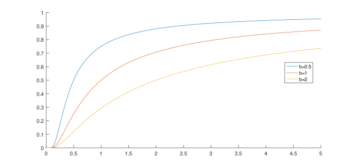
Figure 1. Plot of $q$ for $p=1/2$

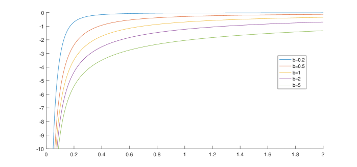
Figure 2. Plot of $\log q$ for $p=1/2$

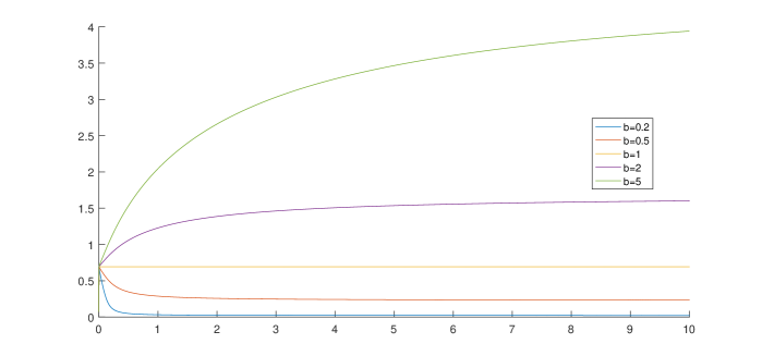
Figure 3. Plot of $\phi$ for $p=1/2$

In the rest of the paper we fix $p\in(0,1)$. We first get the following two propositions, regarding monotonicity and first order asymptotics:

Proposition 1.2.

The function $q$ in (4) is a real analytic and increasing function on $(0,\infty)$. It has limits

$$\lim_{a\rightarrow 0}q(a)=0$$

and

$$\lim_{a\rightarrow\infty}q(a)=1$$

Proposition 1.3.

The function $\phi$ in (5) is real analytic on $(0,\infty)$. It is decreasing if $b<1$, constant if $b=1$ and increasing if $b>1$. It has limits

$$\lim_{a\rightarrow 0}\phi(a)=-\log p$$

and

$$\lim_{a\rightarrow\infty}\phi(a)=\gamma_{b}$$

where $\gamma_{b}$ is the $(1-p)$-quantile of the gamma distribution with parameter $b$.

Then, we investigate the analytic properties of the inverse incomplete beta function deeper. In particular, investigating its logarithm, we obtain the following two results, which consist the main contribution of this paper:

Theorem 1.4.

For fixed $b\in(0,1)$, $\phi$ in (5) is (strictly) convex.

Theorem 1.5.

For fixed $b\in(0,\infty)$, $q$ in (4) is (strictly) log-concave.

Remark 1.6.

One can infer from Figure 1 that $q$ is neither concave nor convex; its reciprocal $1/q$, though, is logarithmically convex by Theorem 1.5, hence also convex. Moreover, based on Figure 3, as well as numerical results, for $b>1$ we conjecture that $\phi$ is concave.

The article is organised in the following way. In section 2 we present some general results regarding $p$-quantiles of more general probability distributions, that have some interest by themselves. For instance, Lemma 2.2 is a generalisation of results concerning monotonicity properties of ratios of power series and polynomials to ratios of integrals. In section 3 we study the monotonicity and limit properties of $q$ and $\phi$ and prove Propositions 1.2 and 1.3. In section 4 we prove convexity of $\phi$ for $b<1$, while in section 5 we prove logarithmic concavity of $q$. In the Appendix, we look into the dependence on the parameter $b$ with $a$ being fixed and translate some of the results in this case.

2. General results on $p$-quantiles of probability distributions

The following lemma is a standard result in measure theory, that lets us interchange integration and differentiation [10, Theorem 6.28]. In the rest of the paper, $\partial_{x}$ denotes differentiation with respect to the variable $x$.

Lemma 2.1.

Let $(\Omega,\mathcal{B},\mu)$ be a measure space, $I\subset\mathbb{R}$ an open interval and $f:I\times\Omega\rightarrow\mathbbm{R}$ a function such that:

1. $a\mapsto f(a,t)$ is differentiable for $\mu$-a.e. $t\in\Omega$

2. $t\mapsto f(a,t)$ is $\mu$-integrable for all $a\in I$

3. $\exists g\in L^{1}(\Omega,\mathrm{d}\mu)$ such that $|\partial_{a}f(a,t)|\leq g(t)$ for all $a\in I$ and $\mu$-a.e. $t\in\Omega$

Then, the function $a\mapsto\int_{\Omega}f(a,t)\mathrm{d}\mu(t)$ is differentiable and

$$\partial_{a}\int_{\Omega}f(a,t)\mathrm{d}\mu(t)=\int_{\Omega}\partial_{a}f(a,t)\mathrm{d}\mu(t)$$

Lemma 2.2.

Let $I\subset\mathbb{R}$ be an open interval, $A\subset\mathbb{R}$ a non-empty Borel set, $\mu$ a $\sigma$-finite Borel measure on $A$ and $u,v:A\rightarrow[0,+\infty)$ measurable functions, not simultaneously $0$. Let $f:I\times A\rightarrow(0,+\infty)$ such that

1. $a\mapsto f(a,t)$ is differentiable for $\mu$-a.e. $t\in A$

2. $t\mapsto u(t)f(a,t)$ and $t\mapsto v(t)f(a,t)$ are $\mu$-integrable for all $a\in I$.

3. For each compact subset $K\subset I$, there exists a function $g_{K}:A\rightarrow[0,+\infty)$ such that $ug_{K},vg_{K}$ are $\mu$-integrable and $|\partial_{a}f(a,t)|\leq g_{K}(t)$ for all $a\in K$ and $\mu$-a.e. $t\in A$.

Let $F:I\rightarrow\mathbb{R}$ be defined by:

$$F(a):=\frac{\int_{A}f(a,t)u(t)\mathrm{d}\mu(t)}{\int_{A}f(a,t)v(t)\mathrm{d}\mu(t)}$$

Then, the following hold:

1. If for all $a\in I$ and for $\mu$-a.e. $t\in A$, $\partial_{a}f(a,t)/f(a,t)$ and $u(t)/v(t)$ both increase or both decrease wrt $t$, then $F$ is increasing.

2. If for all $a\in I$ and for $\mu$-a.e. $t\in A$, $\partial_{a}f(a,t)/f(a,t)$ increases (decreases) wrt $t$ and $u(t)/v(t)$ decreases (increases), then $F$ is decreasing.

Proof.

Let $U(a)=\int_{A}f(a,t)u(t)\mathrm{d}\mu(t)$, $V(a)=\int_{A}f(a,t)v(t)\mathrm{d}\mu(t)$. By the fact that $u(a)\partial_{a}f(a,t)$ and $v(t)\partial_{a}f(a,t)$ are dominated in compact subsets of $I$ by a $\mu$-integrable function of $t$, Lemma 2.1 gives that both $U$ and $V$ are differentiable, and the derivatives can be given by differentiating the integrands. Then, $F^{\prime}$ also exists and hence we need to investigate the derivative

$$F^{\prime}(a)=\frac{U^{\prime}(a)V(a)-U(a)V^{\prime}(a)}{V^{2}(a)}$$

We find

$$U^{\prime}(a)V(a)-U(a)V^{\prime}(a)=$$

$$= \int_{A}\int_{A}u(s)v(t)(\partial_{a}f(a,s)f(a,t)-\partial_{a}f(a,t)f(a,s))\mathrm{d}\mu(s)\mathrm{d}\mu(t)$$

$$= \int_{A}\int_{A\cap\{s<t\}}u(s)v(t)(\partial_{a}f(a,s)f(a,t)-\partial_{a}f(a,t)f(a,s))\mathrm{d}\mu(s)\mathrm{d}\mu(t)$$

$$\qquad+\int_{A}\int_{A\cap\{s>t\}}u(s)v(t)(\partial_{a}f(a,s)f(a,t)-\partial_{a}f(a,t)f(a,s))\mathrm{d}\mu(s)\mathrm{d}\mu(t)$$

$$= \int_{A}\int_{A\cap\{s<t\}}u(s)v(t)(\partial_{a}f(a,s)f(a,t)-\partial_{a}f(a,t)f(a,s))\mathrm{d}\mu(s)\mathrm{d}\mu(t)$$

$$\qquad+\int_{A}\int_{A\cap\{s<t\}}u(t)v(s)(\partial_{a}f(a,t)f(a,s)-\partial_{a}f(a,s)f(a,t))\mathrm{d}\mu(s)\mathrm{d}\mu(t)$$

$$=\int_{A}\int_{A\cap\{s<t\}}(u(s)v(t)-u(t)v(s))(\partial_{a}f(a,s)f(a,t)-\partial_{a}f(a,t)f(a,s))\mathrm{d}\mu(s)\mathrm{d}\mu(t)$$

where in the pre-last equality we have made use of Fubini’s theorem. The last integrand, as $s<t$, is non-negative (non-positive) if $\partial_{a}f/f$ and $u/v$ have the same (opposite) monotonicity properties, which proves the lemma. ∎

Remark 2.3.

In the proceeding Lemma, the same conclusion holds if $u$, $v$ can assume the value zero at the same time, as then, without loss of generality, we can just integrate over the set $A^{\prime}=A\setminus(\{u(t)=0\}\cap\{v(t)=0\})$, which is again a Borel set, and we consider the condition $u/v$ being increasing (or decreasing) in $A^{\prime}$.

Remark 2.4.

Lemma 2.2 is a general case of results concerning monotonicity properties of ratios of power series and polynomials. For instance, it gives [11, Lemma 2.2], if we set $\mu$ to be the counting measure on $\mathbb{N}$.

Lemma 2.5.

Let $I,J$ be two open intervals. Let $f:I\times J\rightarrow(0,\infty)$ such that:

1. $a\mapsto f(a,x)$ is differentiable for a.e. $x\in J$

2. $x\mapsto f(a,x)$ is integrable for all $a\in I$

3. For each compact subset $K\subset I$, there exists an integrable function $g_{K}:J\rightarrow[0,+\infty)$ such that $|\partial_{a}f(a,t)|\leq g_{K}(t)$ for all $a\in K$ and $\mu$-a.e. $t\in A$.

4. The logarithmic derivative of $f$ wrt $a$ is increasing (decreasing) wrt $x$ for a.e. $x$, i.e.

   $$\frac{\partial_{a}f(a,x)}{f(a,x)}\uparrow_{x}(\downarrow_{x})$$

Then, the $p$-quantile $q(a)$ of the probability distribution with density $f(a,x)/\int_{J}f(a,t)dt$ is increasing (decreasing) wrt $a$.

Proof.

We will deal with the case that the logarithmic derivative of $f$ is increasing, and the other case, that it is decreasing, is analogous. Let $x\in J=(c,d)$, where $-\infty\leq c<d\leq+\infty$. Then the cumulative distribution function is

$$F(a;x)=\frac{\int_{c}^{x}f(a,t)\mathrm{d}t}{\int_{c}^{d}f(a,t)\mathrm{d}t}=\frac{\int_{c}^{d}f(a,t)1_{[c,x]}(t)\mathrm{d}t}{\int_{c}^{d}f(a,t)\mathrm{d}t}$$

We set $u(t)=1_{[c,x]}(t)$ and $v(t)=1$. As $u/v=u$ decreases and $\partial_{a}f/f$ increases wrt $t$, by Lemma 2.2 we get that $F$ decreases pointwise wrt $a$. This means

$$\frac{\int^{q(a+h)}_{c}f(a,t)\mathrm{d}t}{\int_{c}^{d}f(a,t)\mathrm{d}t}\geq\frac{\int^{q(a+h)}_{c}f(a+h,t)\mathrm{d}t}{\int_{c}^{d}f(a+h,t)\mathrm{d}t}=p=\frac{\int^{q(a)}_{c}f(a,t)\mathrm{d}t}{\int_{c}^{d}f(a,t)\mathrm{d}t}$$

so that $q(a+h)\geq q(a)$ and hence that the $p$-quantile is increasing. ∎

Remark 2.6.

In Lemma 2.2, if the logarithmic derivative $\partial_{a}f/f$ is strictly monotone (and $u\nequiv v$), it is easy to see from the proof that in the conclusion the ratio of the integrals should also be strictly monotone. Hence, also in Lemma 2.5, if the logarithmic derivative is strictly increasing (decreasing), then the $p$-quantile is also strictly increasing (decreasing).

The following Lemma deals with the question of convergence of $p$-quantiles of a convergent sequence of probability distributions. We denote the extended real line $\mathbbm{R}\cup\{\pm\infty\}$ by $\hat{\mathbbm{R}}$, with its usual topology.

Lemma 2.7.

Let $F_{n}:\hat{\mathbbm{R}}\rightarrow[0,1]$ be a sequence of cumulative distribution functions on $\mathbbm{R}$, extended by $F_{n}(-\infty):=0$ and $F_{n}(+\infty):=1$. Let $q_{n}$ be a $p$-quantile of $F_{n}$, i.e. $F_{n}(q_{n})=p\in(0,1)$, $\forall n\in\mathbbm{N}$. Assume the following conditions:

1. The sequence $(F_{n}(x))_{n\in\mathbbm{N}}$ converges pointwise to a limit $F_{\infty}(x):=\lim_{n\rightarrow\infty}F_{n}(x)$

2. The sequence of $p$-quantiles converges to a limit $q_{\infty}:=\lim_{n\rightarrow\infty}q_{n}\in\hat{\mathbbm{R}}$

Then,

$$q_{\infty}\in[\sup\{x\in\hat{\mathbbm{R}}|F_{\infty}(x)<p\},\inf\{x\in\hat{\mathbbm{R}}|F_{\infty}(x)>p\}]$$ (6)

Thus, if $F_{\infty}$ is continuous, $q_{\infty}$ is a $p$-quantile of $F_{\infty}$.

Proof.

Let some $w\in\hat{\mathbbm{R}}$ such that $F_{\infty}(w)<p$. By condition (i) we have that there is some $n_{0}\in\mathbbm{N}$ such that $\forall n>n_{0}:F_{n}(w)<p=F_{n}(q_{n})$. As each $F_{n}$ is non-decreasing, we have that $\forall n>n_{0}:w<q_{n}$ and hence $q_{\infty}\geqslant w$. As this holds $\forall w\in\{x\in\hat{\mathbbm{R}}|F_{\infty}(x)<p\}$, we get that $q_{\infty}\geqslant\sup\{x\in\hat{\mathbbm{R}}|F_{\infty}(x)<p\}$. In a similar way we may prove that $q_{\infty}\leqslant\inf\{x\in\hat{\mathbbm{R}}|F_{\infty}(x)>p\}$. In case $F_{\infty}$ is continuous, we have $[\sup\{x\in\hat{\mathbbm{R}}|F_{\infty}(x)<p\},\inf\{x\in\hat{\mathbbm{R}}|F_{\infty}(x)>p\}]=\{x\in\mathbbm{R}|F_{\infty}(x)=p\}$, hence then $q_{\infty}$ is a $p$-quantile of $F_{\infty}$. ∎

Remark 2.8.

As $\hat{\mathbbm{R}}$ is compact, $p$-quantiles always have limit points, and the above Lemma shows that convergence of distribution functions for which $p$-quantiles exist implies that all their limit points lie in the interval in (6). This interval either consists of the closure of $F_{\infty}^{-1}(\{p\})$, or, if this set is empty, it degenerates to a point, which is a point of discontinuity of $F_{\infty}$.

Lemma 2.9.

Let $I,J\subset\mathbb{R}$ be open intervals, and $(F(a;x))_{a\in I}$ be a family of cumulative probability distribution functions of $x$ on $J$, having positive densities $f(a;t)$ with respect to Lebesgue measure. Moreover assume that the corresponding densities are real analytic in both variables. Denote the respective $p$-quantiles by $q(a)$. Then, $q$ is a real analytic function of $a$.

Proof.

As the densities are positive functions, the $p$-quantile exists and is unique for each $a$. Hence, the function $q(a)$ is well defined implicitly as the solution $y=q(a)$ to the equation $F(a;y)-p=0$. Let some $y_{0}\in J$ and $a_{0}\in I$ such that $F(a_{0};y_{0})-p=0$. As $F$ is real analytic and $\partial_{y}F(a;y)=f(a;y)\neq 0$, by [12, Theorem 6.1.2] the equation $F(a;y)-p=0$ has a real analytic solution $y=y(a)$ in a neighbourhood of $a_{0}$ such that $F(a_{0};y(a_{0}))-p=0$. By uniqueness of the $p$-quantile this solution must be exactly $q(a)$, and hence $q$ is real analytic. ∎

3. Monotonicity and limits

Proof of Proposition 1.2  Fix $b>0$. As the regularised incomplete beta function $I(x;a,b)$ is real analytic in $x$ and $a$, Lemma 2.9 gives real analyticity of $q$. Let $\beta(a;x):=x^{a-1}(1-x)^{b-1}$. Its logarithmic derivative wrt $a$ is

$$\frac{\partial_{a}\beta(a,b;x)}{\beta(a,b;x)}=\frac{x^{a-1}(1-x)^{b-1}\log x}{x^{a-1}(1-x)^{b-1}}=\log x$$

which is an increasing function of $x$ and Lemma 2.5 gives us that $q$ is also increasing. Its limits at $0$ and $\infty$ are classical results. They can also be obtained by considering limits of the incomplete beta function and using Lemma 2.7. Let, for instance, some limit point $\lim_{n\rightarrow\infty}q(a_{n})=q_{\infty}\in[0,1]$ for a sequence $a_{n}\rightarrow\infty$. Then, the fact that $\lim_{a\rightarrow\infty}I(x;a,b)$ vanishes for $x\in[0,1)$ and is a unit at $x=1$ gives $q_{\infty}=1$, hence $\lim_{a\rightarrow\infty}q(a)=1$. A similar argument shows $\lim_{a\rightarrow 0}q(a)=0$. $\Box$

Proof of Proposition 1.3  By Proposition 1.2 already, $\phi$ can be seen to be a real analytic function. Regarding monotonicity, if $b=1$ then $\phi(a)\equiv-\log p$. Assume $b>1$. By using a change of variables on (4) we get

$$\int_{\phi(a)}^{\infty}e^{-s}(1-e^{-s/a})^{b-1}\mathrm{d}s=p\int_{0}^{\infty}e^{-s}(1-e^{-s/a})^{b-1}\mathrm{d}s$$ (7)

and hence the function $\phi$ is the $(1-p)$-quantile of the distribution with density function

$$x\mapsto\frac{e^{-x}(1-e^{-x/a})^{b-1}}{\int_{0}^{+\infty}e^{-s}(1-e^{-s/a})^{b-1}\mathrm{d}s}$$ (8)

We set $f(a;x):=e^{-x}(1-e^{-x/a})^{b-1}$. The logarithmic derivative of $f$ wrt $a$ is

$$\frac{\partial_{a}f(a;x)}{f(a;x)}=-\frac{(b-1)xe^{-x/a}}{a^{2}(1-e^{-x/a})}$$

The derivative of this wrt $x$ is

$$\partial_{x}\left(\frac{\partial_{a}f(a;x)}{f(a;x)}\right)=\frac{b-1}{a^{3}}\mathrm{e}^{-\frac{x}{a}}\left(a\mathrm{e}^{-\frac{x}{a}}-a+x\right)\left(-1+\mathrm{e}^{-\frac{x}{a}}\right)^{-2}\geq 0$$

as the function $x\mapsto a\mathrm{e}^{-\frac{x}{a}}-a+x$ has positive derivative for $x>0$ and vanishes at $0$. Thus, by Lemma 2.5 we have that $\phi$ is increasing. The case $b<1$ is similar.

For the asymptotic results, we notice that for $a\rightarrow 0$, we have that

$$\lim_{a\rightarrow 0}\frac{e^{-x}(1-e^{-x/a})^{b-1}}{\int_{0}^{\infty}e^{-s}(1-e^{-s/a})^{b-1}\mathrm{d}s}=\frac{e^{-x}}{\int_{0}^{\infty}e^{-s}\mathrm{d}s}=e^{-x}$$

The corresponding distributions, whose $p$-quantiles are equal to $\phi(a)$, converge to the gamma distribution with parameter $1$, and hence by Lemma 2.7 $\lim_{a\rightarrow 0}\phi(a)=-\log p$. Similarly, for $a\rightarrow\infty$

$$\lim_{a\rightarrow\infty}\frac{e^{-x}(1-e^{-x/a})^{b-1}}{\int_{0}^{\infty}e^{-s}(1-e^{-s/a})^{b-1}\mathrm{d}s}=\lim_{a\rightarrow\infty}\frac{e^{-x}}{\int_{0}^{\infty}e^{-s}\frac{(1-e^{-s/a})^{b-1}}{(1-e^{-x/a})^{b-1}}\mathrm{d}s}=\frac{e^{-x}x^{b-1}}{\int_{0}^{\infty}e^{-s}s^{b-1}\mathrm{d}s}$$

hence the distribution converges to the gamma distribution with parameter $b$ and $\lim_{a\rightarrow\infty}\phi(a)=\gamma_{b}$, the $(1-p)$-quantile of the gamma distribution with parameter $b$. $\Box$

4. Convexity of $\phi$ for $b<1$

We rewrite (7) as

$$\int_{0}^{\phi(a)}e^{-s}(1-e^{-s/a})^{b-1}\mathrm{d}s=(1-p)\int_{0}^{\infty}e^{-s}(1-e^{-s/a})^{b-1}\mathrm{d}s$$ (9)

We denote $f(a;s)=e^{-s}(1-e^{-s/a})^{b-1}$ and differentiating the above equation we have

$$\phi^{\prime}(a)f(a;\phi(a))+\int_{0}^{\phi(a)}\partial_{1}f(a;t)\mathrm{d}t=(1-p)\int_{0}^{\infty}\partial_{1}f(a;t)\mathrm{d}t$$ (10)

Differentiating again,

$$\phi^{\prime\prime}(a)f(a;\phi(a))= (1-p)\int_{\phi(a)}^{\infty}\partial_{1}^{2}f(a;t)\mathrm{d}t-p\int_{0}^{\phi(a)}\partial_{1}^{2}f(a;t)\mathrm{d}t$$

$$-(\phi^{\prime}(a))^{2}\partial_{2}f(a;\phi(a))-2\phi^{\prime}(a)\partial_{1}f(a;\phi(a))$$ (11)

where $\partial_{j},j\in\mathbbm{N}$, denotes differentiation wrt to the $j$th variable.

Proof of Theorem 1.4  Let $b\in(0,1)$. By Proposition 1.3 $\phi^{\prime}<0$, and as

$$\partial_{s}f(a;s)=-e^{-s}(1-e^{-s/a})^{b-1}+\frac{b-1}{a}e^{-s}(1-e^{-s/a})^{b-2}e^{-s/a}<0$$

and

$$\partial_{a}f(a;s)=-s\frac{b-1}{a^{2}}e^{-s}(1-e^{-s/a})^{b-2}>0$$

we see that $\phi^{\prime}(a)^{2}\partial_{2}f(a;\phi(a))<0$ and $\phi^{\prime}(a)\partial_{1}f(a;\phi(a))<0$. In order to show that $\phi^{\prime\prime}>0$, using (11) what is left is to show that

$$(1-p)\int_{\phi(a)}^{\infty}\partial_{1}^{2}f(a;t)\mathrm{d}t-p\int_{0}^{\phi(a)}\partial_{1}^{2}f(a;t)\mathrm{d}t\geqslant 0$$ (12)

We shall rewrite the above integrals in another way. We have

$$\int_{\phi(a)}^{\infty}\partial_{1}^{2} f(a;t)\mathrm{d}t=$$

$$= \frac{b-1}{a^{4}}\int_{\phi(a)}^{\infty}2te^{-\frac{2t}{a}}e^{-t}(1-e^{-\frac{t}{a}})^{b-3}\left(\left(a-\frac{t}{2}\right)e^{\frac{t}{a}}+\frac{(b-1)t}{2}-a\right)\mathrm{d}t$$

$$= \frac{2(b-1)}{a}\int_{\frac{\phi(a)}{a}}^{\infty}se^{-as}e^{-2s}(1-e^{-s})^{b-3}\left(\left(1-\frac{s}{2}\right)e^{s}+\frac{b-1}{2}s-1\right)\mathrm{d}s$$

$$= \frac{2(b-1)}{a}\int_{\frac{\phi(a)}{a}}^{\infty}e^{-at}\eta(t)\mathrm{d}t$$

where

$$\eta(x):=xe^{-2x}(1-e^{-x})^{b-3}\left(e^{x}-1-\frac{x}{2}e^{x}+\frac{b-1}{2}x\right)$$ (13)

and similarly

$$\int_{0}^{\phi(a)}\partial_{1}^{2}f(a;t)\mathrm{d}t=\frac{2(b-1)}{a}\int_{0}^{\frac{\phi(a)}{a}}e^{-at}\eta(t)\mathrm{d}t$$

Hence we can rewrite

$$(1-p)\int_{\phi(a)}^{\infty} \partial_{1}^{2}f(a;t)\mathrm{d}t-p\int_{0}^{\phi(a)}\partial_{1}^{2}f(a;t)\mathrm{d}t=$$

$$\frac{2(b-1)}{a}\left((1-p)\int_{\phi(a)/a}^{\infty}e^{-at}\eta(t)\mathrm{d}t-p\int_{0}^{\phi(a)/a}e^{-at}\eta(t)\mathrm{d}t\right)$$ (14)

We now proceed to show (12). We see in Lemma 4.1 that the function

$$w(x):=\left(1-\frac{x}{2}\right)e^{x}+\frac{b-1}{2}x-1$$ (15)

has a unique root $\rho$ on $(0,+\infty)$, and it is positive on $(0,\rho)$ and negative on $(\rho,\infty)$. Assume that $\phi(a)\geqslant\rho a.$ As $w$ and $\eta$ have the same sign, we have that $\int_{\phi(a)/a}^{\infty}e^{-at}\eta(t)\mathrm{d}t<0$. For the other integral, we have

$$\int_{0}^{\phi(a)/a}e^{-at}\eta(t)\mathrm{d}t= \int_{0}^{\rho}e^{-at}\eta(t)\mathrm{d}t+\int_{\rho}^{\phi(a)/a}e^{-at}\eta(t)\mathrm{d}t$$

$$\geq e^{-a\rho}\left(\int_{0}^{\rho}\eta(t)\mathrm{d}t+\int_{\rho}^{\phi(a)/a}\eta(t)\mathrm{d}t\right)$$

$$\geqslant e^{-a\rho}\left(\int_{0}^{\rho}\eta(t)\mathrm{d}t+\int_{\rho}^{\infty}\eta(t)\mathrm{d}t\right)=e^{-a\rho}\int_{0}^{\infty}\eta(t)\mathrm{d}t=0$$

by Lemma 4.2. Hence

$$\frac{2(b-1)}{a}\left((1-p)\int_{\phi(a)/a}^{\infty}e^{-at}\eta(t)\mathrm{d}t-p\int_{0}^{\phi(a)/a}e^{-at}\eta(t)\mathrm{d}t\right)\geqslant 0$$

and by (14), (12) is proved for $\phi(a)\geqslant\rho a.$

Now, assume that $\phi(a)<\rho a$. We define

$$h(a;t):=\frac{\partial_{1}^{2}f(a;t)}{(b-1)f(a;t)}=\frac{2t((a-t/2)e^{t/a}+(b-1)t/2-a)}{a^{4}(e^{t/a}-1)^{2}}$$ (16)

We further denote

$$h_{0}(s):=\frac{a^{2}}{2}h(a;as)=\frac{s((1-s/2)e^{s}+(b-1)s/2-1)}{(e^{s}-1)^{2}}=\frac{sw(s)}{(e^{s}-1)^{2}}$$ (17)

By Lemma 4.3, $h_{0}$ is decreasing on $(0,\rho)$, hence $h(a;s)$ is also decreasing wrt $s$ on $(0,\rho a)$. Hence, for $t\in(0,\phi(a))\subset(0,\rho a)$ we have $h(a;t)>h(a;\phi(a))$. For $t\in(\phi(a),\rho a)$, we analogously have $h(a;\phi(a))>h(a;t)$, and if $t\in(\rho a,\infty)$, then $h(a;\phi(a))>0>h(a;t)$. Hence,

$$(1-p) \int_{\phi(a)}^{\infty}\partial_{1}^{2}f(a;t)\mathrm{d}t-p\int_{0}^{\phi(a)}\partial_{1}^{2}f(a;t)\mathrm{d}t=$$

$$= (b-1)\left((1-p)\int_{\phi(a)}^{\infty}h(a;t)f(a;t)\mathrm{d}t-p\int_{0}^{\phi(a)}h(a;t)f(a;t)\mathrm{d}t\right)$$

$$\geqslant (b-1)h(a;\phi(a))\left((1-p)\int_{\phi(a)}^{\infty}f(a;t)\mathrm{d}t-p\int_{0}^{\phi(a)}f(a;t)\mathrm{d}t\right)=0$$

by (9). Thus (12) is proved. As the RHS of (11) is positive, then $\phi^{\prime\prime}>0$. $\Box$

Lemma 4.1.

Fix $b>0$. The function $w$ in (15) has a unique root $\rho$ on $(0,\infty)$. We have that $w(x)>0$ for $x<\rho$ and $w(x)<0$ for $x>\rho$.

Proof.

We have

$$w^{\prime}(x)=\frac{1-x}{2}e^{x}+\frac{b-1}{2}$$

and

$$w^{\prime\prime}(x)=-\frac{x}{2}e^{x}<0\quad\operatorname{for}x>0$$

Hence $w^{\prime}$ is strictly decreasing, and as $w^{\prime}(0)=b/2$ and $\lim_{x\rightarrow+\infty}w^{\prime}(x)=-\infty$, it changes its sign exactly once and we get that $w$ is initially increasing and then decreasing, concave function. As $w(0)=0$ and $\lim_{x\rightarrow+\infty}w(x)=-\infty$, we get that $w$ has a unique root $\rho\in(0,\infty)$, and $w(x)>0$ for $x<\rho$ and $w(x)<0$ for $x>\rho$. ∎

Lemma 4.2.

For $b>0$, it holds that

$$\int_{0}^{\infty}se^{-2s}(1-e^{-s})^{b-3}\left(e^{s}-1-\frac{s}{2}e^{s}+\frac{b-1}{2}s\right)\mathrm{d}s=0$$

Proof.

In the course of the proof we assume that $b\neq 1,2$, which may be lifted in the end by taking limits. We split the integral into 3 parts. The first one is

$$I_{1}= \int_{0}^{\infty}se^{-2s}(1-e^{-s})^{b-3}(e^{s}-1)\mathrm{d}s$$

$$= \int_{0}^{\infty}se^{-s}(1-e^{-s})^{b-2}\mathrm{d}s$$

$$= -\int_{0}^{\infty}\log(1-e^{-t})e^{-(b-1)t}\mathrm{d}t$$

$$= -\int_{0}^{\infty}\log(1-e^{-t})\left(\frac{1-e^{-(b-1)t}}{b-1}\right)^{\prime}\mathrm{d}t$$

$$= \frac{1}{b-1}\int_{0}^{\infty}\frac{e^{-t}-e^{-bt}}{1-e^{-t}}\mathrm{d}t$$

$$= \frac{\Psi(b)+\gamma}{b-1}$$

where $\Psi:=\Gamma^{\prime}/\Gamma$ is the digamma function (see [3, Chapter 1]). For the second part,

$$I_{2}= \frac{b-1}{2}\int_{0}^{\infty}s^{2}e^{-2s}(1-e^{-s})^{b-3}\mathrm{d}s$$

$$= \frac{b-1}{2(b-2)}\left(\int_{0}^{\infty}s^{2}e^{-s}(1-e^{-s})^{b-2}\mathrm{d}s-2\int_{0}^{\infty}se^{-s}(1-e^{-s})^{b-2}\mathrm{d}s\right)$$

$$= \frac{b-1}{2(b-2)}\int_{0}^{1}\log^{2}t(1-t)^{b-2}\mathrm{d}t-\frac{\Psi(b)+\gamma}{b-2}$$

$$= \frac{b-1}{2(b-2)}\partial_{1}^{2}\mathrm{B}(1,b-1)-\frac{\Psi(b)+\gamma}{b-2}$$

using that $\partial_{1}^{n}\mathrm{B}(a,b)=\int_{0}^{1}t^{a-1}(1-t)^{b-1}\log^{n}t\mathrm{d}t$ for $b>-n$, which is derived by differentiating the integral representation of the beta function for $b>0$ and using the identity principle. Finally,

$$I_{3}= -\frac{1}{2}\int_{0}^{\infty}s^{2}e^{-s}(1-e^{-s})^{b-3}\mathrm{d}s$$

$$= -\frac{1}{2}\int_{0}^{1}(\log t)^{2}(1-t)^{b-3}\mathrm{d}t$$

$$= -\frac{1}{2}\partial_{1}^{2}\mathrm{B}(1,b-2)$$

$$= -\frac{1}{2}\partial_{a}^{2}\left(\mathrm{B}(a,b-1)\frac{a+b-2}{b-2}\right)\bigg{|}_{a=1}$$

$$= -\frac{b-1}{2(b-2)}\partial_{1}^{2}\mathrm{B}(1,b-1)-\frac{\partial_{1}\mathrm{B}(1,b-1)}{b-2}$$

$$= -\frac{b-1}{2(b-2)}\partial_{1}^{2}\mathrm{B}(1,b-1)+\frac{\gamma+\Psi(b)}{(b-2)(b-1)}$$

where we have used that $\partial_{1}\mathrm{B}(1,b-1)=\frac{\gamma+\Psi(b)}{b-1}$. We see that $I_{1}+I_{2}+I_{3}=0$, and the Lemma is proved. ∎

Lemma 4.3.

Fix $b>0$. The function $h_{0}$ in (17) is decreasing between $0$ and its root $\rho\in(0,\infty)$.

Proof.

It is easy to see that $x/(e^{x}-1)$ is decreasing. The rest is also decreasing as

$$\frac{\left(1-\frac{x}{2}\right)e^{x}+\frac{b-1}{2}x-1}{e^{x}-1}=\frac{b}{2}\frac{x}{e^{x}-1}+1-\frac{1}{2}\frac{x(e^{x}+1)}{e^{x}-1}$$

and

$$\left(\frac{x(e^{x}+1)}{e^{x}-1}\right)^{\prime}=\frac{e^{2\hskip 1.18999ptx}-2\hskip 1.69998pte^{x}x-1}{(e^{x}-1)^{2}}\geqslant 0$$

as $\left(e^{2\hskip 1.18999ptx}-2\hskip 1.69998pte^{x}x-1\right)^{\prime}=2e^{x}(e^{x}-x-1)\geqslant 0$ and the numerator vanishes at $0$. Hence, on $(0,\rho)$, $h_{0}$ is the product of two decreasing, positive functions, hence decreasing. ∎

5. Logarithmic concavity of $q$

In this section, we shall prove Theorem 1.5. In order to have a more clear notation, we shall often denote the functions of $a$ ($q,\phi$ and $\psi$), without their argument. Using [8, 8.17.7], we can rewrite (4), as

$$\frac{q^{a}}{a}{}_{2}F_{1}(a,1-b;a+1;q)=p\frac{\Gamma(a)\Gamma(b)}{\Gamma(a+b)}$$ (18)

and expanding the hypergeometric sum,

$$q^{a}\sum_{n=0}^{\infty}\frac{(1-b)_{n}q^{n}}{(a+n)n!}=p\Gamma(b)\frac{\Gamma(a)}{\Gamma(a+b)}$$ (19)

Of course, if $b\in\mathbbm{N}$, the sum above terminates at $b-1$, as $(1-b)_{b}=0$. Using that

$$\frac{(1-b)_{n}}{n!}=\frac{(b-1)(b-1-1)\cdots(b-1-n-1)}{n!}(-1)^{n}=\binom{b-1}{n}(-1)^{n}$$

and denoting

$$\psi:=-\log q$$ (20)

we can rewrite (19) further as

$$e^{-a\psi}\sum_{n=0}^{\infty}\binom{b-1}{n}\frac{(-1)^{n}e^{-n\psi}}{(a+n)}=p\Gamma(b)\frac{\Gamma(a)}{\Gamma(a+b)}$$

that is

$$\sum_{n=0}^{\infty}\frac{\Gamma(a+b)}{\Gamma(a)(a+n)}\binom{b-1}{n}(-1)^{n}e^{-(n+a)\psi}=p\Gamma(b)$$ (21)

We shall show that $\psi$ is convex, which shall imply the logarithmic concavity. The following lemma will be the key to this proof.

Lemma 5.1.

We have that

$$\psi^{\prime}=\sum_{n=0}^{\infty}\frac{1}{a+b+n}Y_{n+b}(\psi)-\sum_{n=0}^{\infty}\frac{1}{a+n}Y_{n}(\psi)$$ (22)

where

$$Y_{c}(\psi):=\frac{\int_{0}^{\psi}e^{ct}(1-e^{-t})^{b-1}\mathrm{d}t}{e^{c\psi}(1-e^{-\psi})^{b-1}}$$ (23)

Proof.

Differentiating (21) we get

$$0= \sum_{n=0}^{\infty}\binom{b-1}{n}(-1)^{n}e^{-(n+a)\psi}\left[\left(\frac{\Gamma(a+b)}{\Gamma(a)(a+n)}\right)^{\prime}-(\psi+(n+a)\psi^{\prime})\frac{\Gamma(a+b)}{\Gamma(a)(a+n)}\right]$$

$$= e^{-a\psi}\sum_{n=0}^{\infty}\binom{b-1}{n}(-1)^{n}e^{-n\psi}\left[\left(\frac{\Gamma(a+b)}{\Gamma(a)(a+n)}\right)^{\prime}-\psi^{\prime}\frac{\Gamma(a+b)}{\Gamma(a)}-\psi\frac{\Gamma(a+b)}{\Gamma(a)(a+n)}\right]$$

Using the fact that $\sum_{n=0}^{\infty}\binom{b-1}{n}(-1)^{n}e^{-n\psi}=(1-e^{-\psi})^{b-1}$, we get

$$\psi^{\prime} (1-e^{-\psi})^{b-1}=$$

$$= \sum_{n=0}^{\infty}\binom{b-1}{n}(-1)^{n}e^{-n\psi}\left(\left(\frac{\Gamma(a+b)}{\Gamma(a)(a+n)}\right)^{\prime}\Bigg{/}\left(\frac{\Gamma(a+b)}{\Gamma(a)}\right)-\frac{\psi}{a+n}\right)$$

$$= \sum_{n=0}^{\infty}\binom{b-1}{n}(-1)^{n}e^{-n\psi}\left(\frac{\Psi(a+b)-\Psi(a)}{a+n}-\frac{1}{(a+n)^{2}}-\frac{\psi}{a+n}\right)$$

$$= \sum_{n=0}^{\infty}\binom{b-1}{n}(-1)^{n}e^{-n\psi}\left(\sum_{k=0}^{\infty}\left(\frac{1}{k+a}-\frac{1}{k+a+b}\right)\frac{1}{a+n}-\frac{1}{(a+n)^{2}}-\frac{\psi}{a+n}\right)$$

$$= \sum_{n=0}^{\infty}\binom{b-1}{n}(-1)^{n}e^{-n\psi}\times$$

$$\left(\sum_{k\neq n}\left(\frac{1}{(k+a)(a+n)}-\frac{1}{(k+a+b)(a+n)}\right)-\frac{1}{(n+a+b)(a+n)}-\frac{\psi}{a+n}\right)$$

$$= \sum_{n=0}^{\infty}\binom{b-1}{n}(-1)^{n}e^{-n\psi}\times$$

$$\sum_{k\neq n}\left(\left(\frac{1}{a+n}-\frac{1}{a+k}\right)\frac{1}{k-n}-\left(\frac{1}{a+n}-\frac{1}{a+k+b}\right)\frac{1}{k+b-n}\right)$$

$$-\sum_{n=0}^{\infty}\left(\binom{b-1}{n}(-1)^{n}e^{-n\psi}\left(\frac{1}{a+n}-\frac{1}{a+n+b}\right)\frac{1}{b}-\frac{\psi}{a+n}\right)$$

$$= \sum_{n=0}^{\infty}\frac{1}{a+n}\binom{b-1}{n}(-1)^{n}e^{-n\psi}\left(\sum_{k\neq n}\left(\frac{1}{k-n}-\frac{1}{k+b-n}\right)\right)$$

$$-\sum_{n=0}^{\infty}\frac{1}{a+n}\binom{b-1}{n}(-1)^{n}e^{-n\psi}\psi+\sum_{n=0}^{\infty}\binom{b-1}{n}(-1)^{n}e^{-n\psi}\times$$

$$\left(\sum_{k\neq n}\left(\frac{1}{a+k+b}\frac{1}{k+b-n}-\frac{1}{a+k}\frac{1}{k-n}\right)+\left(\frac{1}{a+n+b}-\frac{1}{a+n}\right)\frac{1}{b}\right)$$

$$= \sum_{n=0}^{\infty}\frac{1}{a+n}\binom{b-1}{n}(-1)^{n}e^{-n\psi}\left(\sum_{k\neq n}\left(\frac{1}{k-n}-\frac{1}{k+b-n}\right)\right)$$

$$+\sum_{n=0}^{\infty}\left(\frac{1}{a+n+b}-\frac{1}{a+n}\right)\binom{b-1}{n}(-1)^{n}e^{-n\psi}\frac{1}{b}-\sum_{n=0}^{\infty}\frac{1}{a+n}\binom{b-1}{n}(-1)^{n}e^{-n\psi}\psi$$

$$+\sum_{n=0}^{\infty}\sum_{k\neq n}\binom{b-1}{n}(-1)^{n}e^{-n\psi}\left(\frac{1}{a+k+b}\frac{1}{k+b-n}-\frac{1}{a+k}\frac{1}{k-n}\right)$$

$$= \sum_{n=0}^{\infty}\frac{1}{a+n}\binom{b-1}{n}(-1)^{n}e^{-n\psi}\left(\sum_{k\neq n}\left(\frac{1}{k-n}-\frac{1}{k+b-n}\right)\right)$$

$$+\sum_{n=0}^{\infty}\left(\frac{1}{a+n+b}-\frac{1}{a+n}\right)\binom{b-1}{n}(-1)^{n}e^{-n\psi}\frac{1}{b}-\sum_{n=0}^{\infty}\frac{1}{a+n}\binom{b-1}{n}(-1)^{n}e^{-n\psi}\psi$$

$$+\sum_{n=0}^{\infty}\sum_{k\neq n}\binom{b-1}{k}(-1)^{k}e^{-k\psi}\left(\frac{1}{a+n+b}\frac{1}{n+b-k}-\frac{1}{a+n}\frac{1}{n-k}\right)$$

$$= \sum_{n=0}^{\infty}\frac{1}{a+n}\binom{b-1}{n}(-1)^{n}e^{-n\psi}\left(\sum_{k\neq n}\left(\frac{1}{k-n}-\frac{1}{k+b-n}\right)-\frac{1}{b}\right)$$

$$+\sum_{n=0}^{\infty}\frac{1}{a+n}\left(\sum_{k\neq n}\binom{b-1}{k}\frac{(-1)^{k}e^{-k\psi}}{k-n}-\binom{b-1}{n}(-1)^{n}e^{-n\psi}\psi\right)$$

$$+\sum_{n=0}^{\infty}\frac{1}{a+n+b}\sum_{k\neq n}\binom{b-1}{k}\frac{(-1)^{k}e^{-k\psi}}{n+b-k}+\sum_{n=0}^{\infty}\frac{1}{a+n+b}\binom{b-1}{n}(-1)^{n}e^{-n\psi}\frac{1}{b}$$

$$= \sum_{n=0}^{\infty}\frac{1}{a+n}\binom{b-1}{n}(-1)^{n}e^{-n\psi}\left(\sum_{k\neq n}\left(\frac{1}{k-n}-\frac{1}{k+b-n}\right)-\frac{1}{b}\right)$$

$$+\sum_{n=0}^{\infty}\frac{1}{a+n}\left(\sum_{k\neq n}\binom{b-1}{k}\frac{(-1)^{k}e^{-k\psi}}{k-n}-\binom{b-1}{n}(-1)^{n}e^{-n\psi}\psi\right)$$

$$+\sum_{n=0}^{\infty}\frac{1}{a+n+b}\sum_{k=0}^{\infty}\binom{b-1}{k}\frac{(-1)^{k}e^{-k\psi}}{n+b-k}$$

Thus we have

$$\psi^{\prime}= \sum_{n=0}^{\infty}\frac{1}{a+n}X_{n}(\psi)+\sum_{n=0}^{\infty}\frac{1}{a+b+n}Z_{n}(\psi)$$

where

$$X_{n} (\psi):=\Bigg{[}\binom{b-1}{n}(-1)^{n}e^{-n\psi}\left(\sum_{k\neq n}\left(\frac{1}{k-n}-\frac{1}{k+b-n}\right)-\frac{1}{b}\right)$$

$$+\sum_{k\neq n}\binom{b-1}{k}(-1)^{k}e^{-k\psi}\frac{1}{k-n}-\binom{b-1}{n}(-1)^{n}e^{-n\psi}\psi\Bigg{]}/(1-e^{-\psi})^{b-1}$$

and

$$Z_{n}(\psi):=\left(\sum^{\infty}_{k=0}\binom{b-1}{k}(-1)^{k}e^{-k\psi}\frac{1}{n+b-k}\right)/(1-e^{-\psi})^{b-1}$$

By Lemma 5.2 and

$$\partial_{\psi}\left(\sum^{\infty}_{k=0}\binom{b-1}{k}(-1)^{k}e^{(n+b-k)\psi}\frac{1}{n+b-k}\right)=e^{(n+b)\psi}(1-e^{-\psi})^{b-1}$$

we have that

$$\sum^{\infty}_{k=0}\binom{b-1}{k}(-1)^{k}e^{(n+b-k)\psi}\frac{1}{n+b-k}=\int_{0}^{\psi}e^{(n+b)t}(1-e^{-t})^{b-1}\mathrm{d}t$$

and hence we get

$$Z_{n}(\psi)= e^{-(n+b)\psi}\left(\sum^{\infty}_{k=0}\binom{b-1}{k}(-1)^{k}e^{(n+b-k)\psi}\frac{1}{n+b-k}\right)/(1-e^{-\psi})^{b-1}$$

$$= e^{-(n+b)\psi}\int_{0}^{\psi}e^{(n+b)t}(1-e^{-t})^{b-1}\mathrm{d}t/(1-e^{-\psi})^{b-1}$$

$$= \frac{\int_{0}^{\psi}e^{(n+b)t}(1-e^{-t})^{b-1}\mathrm{d}t}{e^{(n+b)\psi}(1-e^{-\psi})^{b-1}}=Y_{n+b}(\psi)$$

Similarly, Lemma 5.2 and

$$\partial_{\psi}\left(\sum_{k\neq n}\binom{b-1}{k}(-1)^{k}e^{-(k-n)\psi}\frac{1}{k-n}-\binom{b-1}{n}(-1)^{n}\psi\right)=-e^{n\psi}(1-e^{-\psi})^{b-1}$$

give

$$X_{n}(\psi)= -\frac{\int_{0}^{\psi}e^{nt}(1-e^{-t})^{b-1}\mathrm{d}t}{e^{n\psi}(1-e^{-\psi})^{b-1}}=-Y_{n}(\psi)$$

hence (22) is proved. ∎

Lemma 5.2.

For $n\in\mathbbm{N}$ and $b>0$, we have

$$\sum^{\infty}_{k=0}\binom{b-1}{k}\frac{(-1)^{k}}{n+b-k}=0$$ (24)

and

$$\sum_{k\neq n}\binom{b-1}{k}(-1)^{k}\frac{1}{k-n}=-\binom{b-1}{n}(-1)^{n}\left(\sum_{k\neq n}\left(\frac{1}{k-n}-\frac{1}{k+b-n}\right)-\frac{1}{b}\right)$$ (25)

Proof.

For $z\in\mathbbm{C}\setminus\{0,-1,-2,\ldots\}$ we have, applying [3, Theorem 2.2.2],

$$\sum^{\infty}_{k=0}\binom{b-1}{k}\frac{(-1)^{k}}{k+z}= \frac{1}{z}\sum^{\infty}_{k=0}\frac{(1-b)_{k}(z)_{k}}{k!(z+1)_{k}}=\frac{{}_{2}F_{1}(1-b,z;z+1;1)}{z}$$

$$= \frac{\Gamma(z+1)\Gamma(b)}{z\Gamma(z+b)}=\frac{\Gamma(z)\Gamma(b)}{\Gamma(z+b)}$$

Hence, we get

$$\sum^{\infty}_{k=0}\binom{b-1}{k}\frac{(-1)^{k}}{n+b-k}=\lim_{z\rightarrow n}\sum^{\infty}_{k=0}\binom{b-1}{k}\frac{(-1)^{k}}{z+b-k}=-\lim_{z\rightarrow n}\frac{\Gamma(b)\Gamma(-z-b)}{\Gamma(-z)}=0$$

proving (24). For (25), assume $z\in\mathbbm{C}\setminus\mathbbm{N}$ and let

$$\binom{b-1}{n}(-1)^{n}\left(\sum_{k\neq n}\left(\frac{1}{k-z}-\frac{1}{k+b-z}\right)-\frac{1}{n+b-z}\right)+\sum_{k\neq n}\binom{b-1}{k}\frac{(-1)^{k}}{k-z}$$

$$= \binom{b-1}{n}(-1)^{n}\left(\sum^{\infty}_{k=0}\left(\frac{1}{k-z}-\frac{1}{k+b-z}\right)-\frac{1}{n-z}\right)+\sum_{k=0}^{\infty}\binom{b-1}{k}\frac{(-1)^{k}}{k-z}-\binom{b-1}{n}\frac{(-1)^{n}}{n-z}$$

$$= \binom{b-1}{n}(-1)^{n}\left(\Psi(b-z)-\Psi(-z)-\frac{1}{n-z}\right)+\frac{\Gamma(b)\Gamma(-z)}{\Gamma(b-z)}-\binom{b-1}{n}\frac{(-1)^{n}}{n-z}$$

$$= \binom{b-1}{n}(-1)^{n}\left(\Psi(b-z)-\Psi(1+z)-\pi\frac{\cos(\pi z)}{\sin(\pi z)}-\frac{1}{n-z}\right)+\frac{\Gamma(b)\Gamma(-z)}{\Gamma(b-z)}-\binom{b-1}{n}\frac{(-1)^{n}}{n-z}$$

where we have used the reflection formula for the digamma function. We have, using that $\operatorname{Res}\left(\frac{\pi\cos\pi z}{\sin\pi z},n\right)=1$, that

$$\lim_{z\rightarrow n}\left(\Psi(b-z)-\Psi(1+z)-\pi\frac{\cos(\pi z)}{\sin(\pi z)}-\frac{1}{n-z}\right)=\Psi(b-n)-\Psi(1+n)$$

Furthermore, using de L’Hôpital’s rule, we get

$$\lim_{z\rightarrow n} \left(\frac{\Gamma(b)\Gamma(-z)}{\Gamma(b-z)}-\binom{b-1}{n}\frac{(-1)^{n}}{n-z}\right)=$$

$$= \lim_{z\rightarrow n}\left(-\frac{\Gamma(b)}{\Gamma(b-z)\Gamma(1+z)}\frac{\pi}{\sin\pi z}-\binom{b-1}{n}\frac{(-1)^{n}}{n-z}\right)$$

$$= \lim_{z\rightarrow n}\frac{\frac{\Gamma(b)}{\Gamma(b-z)\Gamma(1+z)}(n-z)-\binom{b-1}{n}(-1)^{n}\frac{\sin\pi z}{\pi}}{\frac{\sin\pi z}{\pi}(n-z)}$$

$$= \lim_{z\rightarrow n}\frac{\left(\frac{\Gamma(b)}{\Gamma(b-z)\Gamma(1+z)}\right)^{\prime}(n-z)+\frac{\Gamma(b)}{\Gamma(b-z)\Gamma(1+z)}+\binom{b-1}{n}(-1)^{n}\cos\pi z}{\frac{\sin\pi z}{\pi}-(n-z)\cos\pi z}$$

$$= \lim_{z\rightarrow n}\frac{\left(\frac{\Gamma(b)}{\Gamma(b-z)\Gamma(1+z)}\right)^{\prime\prime}(n-z)+\left(\frac{\Gamma(b)}{\Gamma(b-z)\Gamma(1+z)}\right)^{\prime}+\pi\binom{b-1}{n}(-1)^{n}\sin\pi z}{\cos\pi z+(n-z)\pi\sin\pi z+\cos\pi z}$$

$$= \frac{\frac{\Gamma(b)}{\Gamma(b-n)\Gamma(1+n)}(\Psi(1+n)-\Psi(b-n))}{2\cos\pi n}$$

$$= (-1)^{n}\binom{b-1}{n}(\Psi(1+n)-\Psi(b-n))$$

hence getting (25). ∎

Lemma 5.3.

Let $b>1$ and $c>0$. Then, $Y_{c}$ is increasing on $(0,\infty)$. Moreover, $Y_{c}(x)$, $Y^{{}^{\prime}}_{c}(x)$ are decreasing wrt $c$ for fixed $x$.

Proof.

We rewrite

$$\frac{\int_{0}^{x}e^{ct}(1-e^{-t})^{b-1}\mathrm{d}t}{e^{cx}(1-e^{-x})^{b-1}}= \int_{0}^{x}e^{c(t-x)}\left(\frac{1-e^{-t}}{1-e^{-x}}\right)^{b-1}\mathrm{d}t$$

$$= \int_{0}^{x}e^{c(t-x)}\left(\frac{e^{x}-e^{x-t}}{e^{x}-1}\right)^{b-1}\mathrm{d}t$$

$$= \int_{0}^{x}e^{-cv}\left(\frac{e^{x}-e^{v}}{e^{x}-1}\right)^{b-1}\mathrm{d}v$$

Differentiating, we get

$$\Bigg{(}\int_{0}^{x}e^{-cv}\left(\frac{e^{x}-e^{v}}{e^{x}-1}\right)^{b-1}\mathrm{d}t\Bigg{)}^{\prime}= \int_{0}^{x}e^{-cv}\partial_{x}\left(\frac{e^{x}-e^{v}}{e^{x}-1}\right)^{b-1}\mathrm{d}v$$

$$= \int_{0}^{x}e^{-cv+x}(b-1)\left(\frac{e^{x}-e^{v}}{e^{x}-1}\right)^{b-2}\frac{e^{v}-1}{(e^{x}-1)^{2}}\mathrm{d}v$$

and this completes the proof. ∎

Proof of Theorem 1.5  We shall show the convexity of $\psi=-\log q$, which is equivalent to logarithmic concavity of $q$. The case $b<1$ is given by Theorem 1.4, as $a\psi^{\prime\prime}=\phi^{\prime\prime}-2\psi^{\prime}>0$. For $b=1$, we have $\psi=\frac{\log(1/p)}{a}$ hence $\psi^{\prime\prime}=0$. For $b>1$, differentiating (22) we get

$$\psi^{\prime\prime}= \sum_{n=0}^{\infty}\frac{1}{(a+n)^{2}}Y_{n}(\psi)-\sum_{n=0}^{\infty}\frac{1}{(a+b+n)^{2}}Y_{n+b}(\psi)+$$

$$\left(\sum_{n=0}^{\infty}\frac{1}{a+b+n}Y^{\prime}_{n+b}(\psi)-\sum_{n=0}^{\infty}\frac{1}{a+n}Y^{\prime}_{n}(\psi)\right)\psi^{\prime}>0$$

using that $\psi^{\prime}<0$ and Lemma 5.3. $\Box$

Remark 5.4.

We notice that (22) also gives

$$q^{\prime}=\sum_{n=0}^{\infty}\frac{1}{a+b+n}\frac{\int_{q}^{1}t^{-n-b-1}(1-t)^{b-1}\mathrm{d}t}{q^{-n-b-1}(1-q)^{b-1}}-\sum_{n=0}^{\infty}\frac{1}{a+n}\frac{\int_{q}^{1}t^{-n-1}(1-t)^{b-1}\mathrm{d}t}{q^{-n-1}(1-q)^{b-1}}$$ (26)

Appendix

Finally, we want to see how the $p$-quantile depends on the second parameter of the beta distribution. For clarity, from now on we denote the $p$-quantile of the beta distribution with parameters $a$ and $b$ by $q_{p}(a,b)$. We shall consider $a$ constant, and try to relate $q$ as a function of $b$ with the previous results.

A simple change of variables $s=1-t$ gives the functional relation

$$I(x;a,b)=1-I(1-x;b,a)$$ (27)

which implies

$$p=I(q_{p}(a,b);a,b)=1-I(q_{p}(a,b);b,a)\Rightarrow I(q_{p}(a,b);b,a)=1-p=I(q_{1-p}(a,b);b,a)$$

and using the uniqueness of the $p$-quantile we get

$$q_{p}(a,b)=1-q_{1-p}(b,a)$$ (28)

Hence, by Proposition 1.2, we get that $q_{p}$ is decreasing in $b$ and

$$\lim_{b\rightarrow 0}q_{p}(a,b)=1$$

$$\lim_{b\rightarrow\infty}q_{p}(a,b)=0$$

Moreover, we have

$$(1-q_{p}(a,b))^{b}=q_{1-p}(b,a)^{b}=e^{-\varphi_{1-p}(b)}$$ (29)

where $\varphi_{1-p}(b)=-b\log q_{1-p}(b,a)$, hence the behaviour of $q_{p}(a,b)$ as a function of $b$ can again be studied similarly through the function $\varphi_{p}$. We also easily see that $b\mapsto 1-q_{p}(a,b)$ is log-concave. We remark that numerical evidence shows that $b\mapsto q_{p}(a,b)$ itself is not (log-)concave/convex. However, the function $b\mapsto\varphi_{p}(b)$ seems to be convex.

References

[1]
J. A. Adell and P. Jodrá.
On a Ramanujan equation connected with the median of the gamma
distribution.
Trans. Amer. Math. Soc., 360:3631–3644, 2008.
[2]
S. E. Alm.
Monotonicity of the difference between median and mean of gamma
distributions and of a related ramanujan sequence.
Bernoulli, 9(2):351–371, 2003.
[3]
G. E. Andrews, R. Askey, and R. Roy.
Special Functions.
Cambridge University Press, 1999.
Cambridge Books Online.
[4]
C. Berg and H. L. Pedersen.
The chen-rubin conjecture in a continuous setting.
Methods and Applications of Analysis, 13, 2006.
[5]
C. Berg and H. L. Pedersen.
Convexity of the median in the gamma distribution.
Ark. Mat., 46, 2008.
[6]
J. Chen and H. Rubin.
Bounds for the difference between median and mean of gamma and
Poisson distributions.
Stat. Probab. Lett., 4:281–283, 1986.
[7]
K. P. Choi.
On the medians of gamma distributions and an equation of ramanujan.
Proceedings of the American Mathematical Society,
121(1):245–251, 1994.
[8]NIST Digital Library of Mathematical Functions.
http://dlmf.nist.gov/, Release 1.0.12 of 2016-09-09.
F. W. J. Olver, A. B. Olde Daalhuis, D. W. Lozier, B. I. Schneider,
R. F. Boisvert, C. W. Clark, B. R. Miller and B. V. Saunders, eds.
[9]
D. B. Karp.
Normalized incomplete beta function: Log-concavity in parameters and
other properties.
Journal of Mathematical Sciences, 217(1):91–107, Aug 2016.
[10]
A. Klenke.
Probability Theory: A Comprehensive Course.
Universitext. Springer London, 2007.
LCCB: 2007939558.
[11]
S. Koumandos and H. L. Pedersen.
On the asymptotic expansion of the logarithm of barnes triple gamma
function.
Mathematica Scandinavica, 105, 2009.
[12]
S.G. Krantz and H.R. Parks.
The Implicit Function Theorem: History, Theory, and
Applications.
Birkhäuser, 2002.
[13]
M. E. Payton, L. J. Young, and J. H. Young.
Bounds for the difference between median and mean of beta and
negative binomial distributions.
Metrika, 36(1):347–354, 1989.
[14]
N.M. Temme.
Asymptotic inversion of the incomplete beta function.
Journal of Computational and Applied Mathematics, 41(1):145 –
157, 1992.