The foot points of the Giant Molecular Loops in the Galactic center region

Abstract

Aims. To reveal the morphology, chemical composition, kinematics and to establish the main processes prevalent in the gas at the foot points of the giant molecular loops (GMLs) in the Galactic center region

Methods. Using the 22-m Mopra telescope, we mapped the M$-3.8+0.9$ molecular cloud, placed at the foot points of a giant molecular loop, in 3-mm range molecular lines. To derive the molecular hydrogen column density, we also observed the ¹³CO $(2-1)$ line at 1 mm using the 12-m APEX telescope. From the 3 mm observations 12 molecular species were detected, namely HCO⁺, HCN, H¹³CN, HNC, SiO, CS, CH₃OH, N₂H⁺, SO, HNCO, OCS, and HC₃N.

Results. Maps revealing the morphology and kinematics of the M$-3.8+0.9$ molecular cloud in different molecules are presented. We identified six main molecular complexes. We derive fractional abundances in 11 selected positions of the different molecules assuming local thermodynamical equilibrium.

Conclusions. Most of the fractional abundances derived for the M$-3.8+0.9$ molecular cloud are very similar over the whole cloud. However, the fractional abundances of some molecules show significant difference with respect to those measured in the central molecular zone (CMZ). The abundances of the shock tracer SiO are very similar between the GMLs and the CMZ. The methanol emission is the most abundant specie in the GMLs. This indicates that the gas is likely affected by moderate $\sim$ 30 km s^-1 or even high velocity (50 km s^-1) shocks, consistent with the line profile observed toward one of the studied position. The origin of the shocks is likely related to the flow of the gas throughout the GMLs towards the foot points.

1 Introduction

The central regions of galaxies interact and exchange matter and radiation with their surroundings. This interaction strongly affects and modifies the physical properties and the chemistry in their nuclear regions. Due to its proximity, the central region of the Milky Way allows detailed high resolution studies of the role of a variety of phenomena, namely magnetic loops (Fukui et al. 2006), galactic winds (Bland-Hawthorn & Cohen 2003), gas accretion by e.g., a barred Galactic model (Binney et al. 1991).
The molecular component of the Galactic center (GC) region (i.e., the inner $\sim 1$ kpc of the Galaxy in the context of this work) is composed by a large molecular complex in the central $\sim 500$ pc known as the “Central Molecular Zone” (CMZ, Morris & Serabyn 1996), and several molecular clouds with high CO luminosity and large velocity dispersion (Bitran et al. 1997) outside the CMZ from $l\sim-6$ ^∘to $l\sim 6$ ^∘and $b\sim-1$^∘to $b\sim 2$^∘(Fig. 1) that are also placed in the GC region. There are many molecular line emission surveys of the CMZ (e.g., Jones et al. 2012), but few of them cover the molecular clouds beyond the CMZ. Bitran et al. (1997) observed a region of $-12$^∘$<l<$ $12$^∘, $-2$^∘$<b<$ $2$^∘ in CO$(1-0)$, identifying 5 large velocity width and high CO luminosity clumps outside the CMZ located in the GC. Fukui et al. (2006) extended the coverage of maps in this line to a larger latitude range with better spatial resolution and identified huge loop structures in the negative velocity range from $-180$  km s^-1to $-40$  km s^-1with filamentary structure with a width of $\sim 30$ pc and a length of $\sim 400$ pc and heights of $\sim 2$^∘  from the Galactic plane. These features are coherent in velocity, with velocity gradients of $0.2-0.35$ km s^-1pc^-1. Fukui et al. (2006) proposed that these “giant molecular loops” (GMLs) placed in the GC are formed by a magnetic buoyancy caused by a Parker instability. According to the model presented in Fukui et al. (2006), the gas of the loops would flow down their sides, along the magnetic field lines, and join with the gas layer of the Galactic plane, generating shock fronts at the “foot points” of the loops. The presence of shocked gas is supported by the broad velocity features of $\sim$ 40 to 80  km s^-1 width observed by Bitran et al. (1997) and Fukui et al. (2006).
Additional evidence of shocked gas at the “foot points”, comes from a survey of the GC region in HCO${}^{+}(1-0)$, H¹³CO${}^{+}(1-0)$, and SiO$(2-1)$ lines (Riquelme et al. 2010b). The mapped area ($-5{{}^{\circ}}.75<l<5{{}^{\circ}}.63$ and $-0{{}^{\circ}}.7<b<1{{}^{\circ}}.35$) includes the CMZ and the 5 clumps observed by Bitran et al. (1997) mentioned above. They found an enhancement of the SiO emission (an archetypical tracer of shocked gas) at the “foot points” zones with respect to HCO⁺. This strongly suggests the presence of shocks (Martín-Pintado et al. 1992, 1997).

Despite there are still no confirmatory magnetic field measurements in these features, multi-transitional CO observations towards both the foot points and the complete loops, and magnetohydrodynamical simulations support the GMLs scenario. Table 1 summarizes the characteristics of the GMLs. Torii et al. (2010a) studied in detail the foot point of the GMLs towards $l\sim 356^{\circ}$ (hereafter “M$-3.8+0.9$ molecular cloud”). They identified and analyzed several features including two “U-shapes”, which they propose to be formed by the merging of two downward, i.e., to lower latitude flows between two loops as predicted by magneto-hydrodynamics numerical simulations (Takahashi et al. 2009; Machida et al. 2009). Fujishita et al. (2009) discovered the “loop 3”, placed in the positive-velocity range in $l\simeq 354{{}^{\circ}}-359{{}^{\circ}}$, and Fukui et al. (2006) proposed the existence of other GMLs connecting molecular clouds with large velocity widths at $l\sim 1{{}^{\circ}}.3,3{{}^{\circ}}.2$ (Bania et al. 1986), and $5{{}^{\circ}}.3$. Kaneda et al. (2012) found that the polycyclic aromatic hydrocarbon (PAH) infrared emission at 9 $\mu$m is spatially correlated with the loops; however, it is suppressed in the foot points as compared with the IRAS 100 $\mu$m emission. This suggested the destruction of PAHs relative to sub-micron dust grains by shocks. Isotope studies (Riquelme et al. 2010a) suggest that gas has been accreted towards the foot point of the loops, and metastable inversion transitions of the ammonia (Riquelme et al. 2013) revealed high kinetic temperatures ($>90$ K) in the “foot points” of the loop at $l\sim 5{{}^{\circ}}.2$. Fig. 1 presents an overview of the large scale GC region, showing the CMZ, the five molecular clouds outside the CMZ, and the location of the giant molecular loops discussed in this paper.
This paper presents high angular resolution mapping of 3-mm molecular lines toward the M$-3.8+0.9$ molecular cloud, placed at the foot points of the molecular loops discovered by Fukui et al. (2006) in the GC. These observations allow us to derive the morphology, chemistry and the kinematics of both the quiescent and the shocked gas at small spatial scales of order 1 pc. The projected distance from Sgr A* of the M$-3.8+0.9$ molecular cloud is 564 pc, assuming a distance of 8.5 kpc (the IAU recommended value).

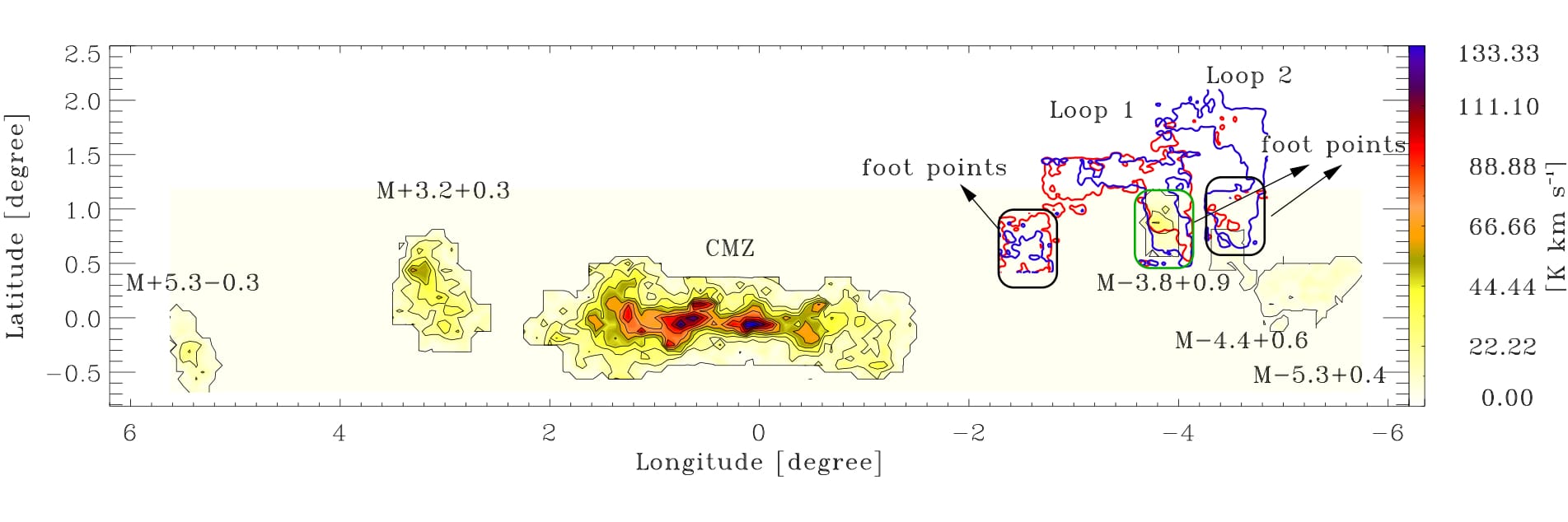
Figure 1: Overview of the large scale GC region showing the features discussed in this work. The CMZ and five molecular clouds are indicated by the HCO⁺ $(1-0)$ emission from Riquelme et al. (2010b). Loops 1 and 2 are plotted in the CO $(2-1)$ emission from Kudo et al. (2011). Loop 1 is integrated in the velocity range $-180$ to $-90$  km s^-1(blue contour), and loop 2 from $-90$ to $-40$  km s^-1(red contour). The foot points are indicated with the black ellipse. The green ellipse shows the M$-3.8+0.9$ molecular cloud studied in this work.

Table 1: Summary of the characteristics of the giant molecular loops

Loop	Longitude range	Latitude range	Velocity range	Mass	Foot point location
	[Degree]	[Degree]	[km $s^{-1}$]	M${}_{\mathord{\odot}}$
Loop 1	$355{{}^{\circ}}.8$ – $358{{}^{\circ}}.0$	$0^{\circ}.5$ – $1^{\circ}.6$	$-180$ – $-90$	$7-12\times 10^{5}$	$(l,b)\sim(356^{\circ},1^{\circ})$ and $(l,b)\sim(357^{\circ}.4,0.^{\circ}8)$
Loop 2	$355{{}^{\circ}}.2$ – $356^{\circ}.6$	$0^{\circ}.6$ – $2^{\circ}.2$	$-90$ – $-40$	$8-16\times 10^{5}$	$(l,b)\sim(355^{\circ}.4,0^{\circ}.8)$ and $(l,b)\sim(356^{\circ}.1,0^{\circ}.8)$
Loop 3	$354{{}^{\circ}}-359{{}^{\circ}}$	$0^{\circ}$ – $2^{\circ}$	$30$ – $160$	$3\times 10^{3}$	$(l,b)\sim 355{{}^{\circ}}.5,0{{}^{\circ}}.7)$,$(l,b)\sim 359{{}^{\circ}},0{{}^{\circ}}.6)$

2 Observations and data reduction

2.1 Mopra observations and data reduction

The observations were carried out using the 22-m Mopra telescope during September 2008 and August 2009. Located in the Southern hemisphere, and due to its high angular resolution and wide-bandwidth spectrometer, the Mopra telescope offered excellent capabilities to establish the chemical abundances of the molecular gas at the foot points of the GC loops. We used the digital mode filter bank MOPS in broad-band mode, covering 8 GHz of bandwidth simultaneously in four $2.2$ GHz sub-bands, each of them with $8192$ channel spaced by $0.27$ MHz. Two polarizations were measured simultaneously.

We mapped a selected region of the M$-3.8+0.9$ molecular cloud (Riquelme et al. 2010b) using the on-the-fly (OTF) mapping mode (Ladd et al. 2005; Mangum et al. 2007). Observations of tiles of $5^{\prime}\times 5^{\prime}$ size with overlaps of $30^{\prime\prime}$ were used to cover the complete region. The complete maps covered the region of $356{{}^{\circ}}.06<l<356{{}^{\circ}}.29$ and $0{{}^{\circ}}.645<b<1{{}^{\circ}}.1$. We used position switching mode with the off position placed at $(l,b)=(356{{}^{\circ}}.375,1{{}^{\circ}}.5)$, which was checked to be free of emission, and observed in symmetric mode (one off per OTF scan). The spacing between scan rows was $12^{\prime\prime}$, and each tile of $5\times 5$ ${\rm arcmin}^{2}$ took 55 min to complete. To establish pointing parameter corrections we observed before each map the SiO maser source AH Sco. The spectra were read out with 2 seconds of integration time. The system temperature was calibrated with a noise diode and a hot/cold load (paddle) every 30 min. We observed two frequency setups, one centered at $89.41$ GHz and the other at $99.72$ GHz covering the ranges between $85.275$ and $93.555$ GHz and from $95.585$ to $103.866$ GHz.

The data were reduced using the LIVEDATA and GRIDZILLA packages. LIVEDATA is the processing software used to apply system temperature calibration, bandpass calibration, heliocentric correction, spectral smoothing and to write out the data in sdfits (Garwood 2000) format. GRIDZILLA is a regridding software package to convert the sdfits files to the FITS data cube (Jones et al. 2008). A first order polynomial baseline was subtracted with LIVEDATA, and the data were regridded with GRIDZILLA into data cubes, using a Gaussian smoothing interpolation.
The final spatial resolution of the data cubes is between $49^{\prime\prime}$ and $51^{\prime\prime}$ at 115 and 86 GHz respectively, which is obtained after convolution of the Mopra beam width of $33\pm 3^{\prime\prime}$ at 115 GHz and $36\pm 3^{\prime\prime}$ from 86 to 100 GHz, as measured using Jupiter in 2004 (Ladd et al. 2005), with a Gaussian of $36^{\prime\prime}$ full width half maximum (FWHM). This FWHM for the Gaussian size improves the signal-to-noise of the data, albeit with a modest loss in spatial resolution. We calibrated the data in the main beam brightness temperature ($T_{\rm mb}$) scale. The main beam efficiency of Mopra varies between 0.49 at 86 GHz and 0.42 at 115 GHz. However, to convert to $T_{\rm mb}$ we used the values for the extended beam efficiency which are more appropriate for the extended emission of the Galactic center region (0.65 at 86 GHz and 0.55 at 115 GHz) (Ladd et al. 2005). The spectral resolution of the data is 269.5 kHz (0.94 – 0.78  km s^-1). One data cube per molecular line was made. The size of the pixel is $15$ arc sec in the final cube. We produces 13 data cubes for the detected molecules in the Mopra survey (see Table 2). In 5 of those data cubes (CS, SiO, HC3N-10-9, H13CN, CH3OH), it was necessary to subtract 3^rd order baselines for $\sim 20$ % of the data using MADCUBAIJ software.

2.2 APEX observations and data reduction

The $J=2-1$ rotational transition of ¹³CO was mapped using the 12-m Atacama Pathfinder EXperiment (APEX) telescope (Güsten et al. 2006), covering a similar region as the Mopra observations (see Fig. 3). The observations were carried out on 24 Jun, 1, 2 and 3 July 2014 under the APEX project code M-093.F-008-2014 using the APEX-1 (SHIFI) receiver (Vassilev et al. 2008) and the eXtended bandwidth Fast Fourier Transform Spectrometer (XFFTS) backend (Klein et al. 2012). OTF position-switching observing mode was used, with a close off position slightly contaminated with ¹³CO emission ($\alpha$(J2000): $17{\rm h}33{\rm m}13.0{\rm s}$, $\delta$(J2000): $-31{{}^{\circ}}30^{\prime}13^{\prime\prime}.9$) mainly at the velocity range from $-10$ to 30 km s^-1 with an intensity peak $T_{\rm MB}=0.6$ K, 100 to 110 km s^-1 with an intensity peak of $T_{\rm MB}=0.2$ K, and in much less amount from $-80$ to $-70$ km s^-1 and from $-50$ to $-20$ km s^-1 with $T_{\rm MB}<0.1$ K. This contamination was corrected later with observations against a clean off position (RA(J2000): $17{\rm h}30{\rm m}48.0{\rm s}$, DEC(J2000): $-31{{}^{\circ}}11^{\prime}48^{\prime\prime}.1$). This observing strategy ensure flat baselines across the map. The pointing was checked every 1.5-2 hours on IRAS17150-3224; corrections smaller than $2^{\prime\prime}$ were determined. The system temperature ($T_{{\rm sys}}$) ranged from 125 to 204 K, with an average value of 155 K. The calibration was done using the standard APEX calibration procedure, with an estimated error of $\sim 10\%$.

The data was reduced using the CLASS package from the GILDAS software. The antenna temperature ($T_{\rm A}^{*}$) was converted to $T_{\rm MB}$ using the Ruze formula with B${}_{0}=0.69$ and $\sigma=0.19$ for an extended source (see Appendix B). All spectra were taken into account since the observed rms noise was in all cases lower than 1.5$\times$ the theoretical noise (Ao et al. 2013; Ginsburg et al. 2016) . Third order polynomial baselines were subtracted for the OTF mapping observations of the M$-3.8+0.9$ molecular cloud, and a fifth order polynomial baselines for the position switching observations in the reference position. Then, each individual spectrum for the mapping was combined with the reference position spectrum using the accumulate function in CLASS with an equal weighting. In this way, the baseline time-dependence is removed. Since line widths $>10$  km s^-1were expected, the final spectra were smoothed with the box function in CLASS to reach a final velocity resolution of $1.04$  km s^-1which is more than enough to resolve all the kinematic structures of this molecular cloud. The data were regridded in equatorial coordinates and then converted to Galactic coordinates for comparison with the Mopra data using standard CLASS routines. The average root-mean-square (rms) noise for the spectra in the data cube is 127 mK at a velocity resolution of $\approx 1$ km s^-1. The final data cube was corrected for additional baseline subtraction using MADCUBAIJ software in small regions when needed (2-3 order polynomial base line subtraction in the 30% of the data).

3 Results

Following the list of most prominent 3 mm wavelength molecular lines observed in Sgr B2 by Jones et al. (see their Table 2 in 2008), we made one data cube per molecule. Tables 2 and 3 show the molecules and the rms noise values reached in each molecular line cube. The results are presented both in the main text and in the Appendices A to D.

Table 2: List of imaged molecular transitions, their rms noise level ($T_{\rm A}^{*}$) and the main beam efficiency.

Molecule	Transition	Rest. Freq.	rms3	$\eta_{\rm MB}$
		[GHz]	[mK]
H13CN	$1-0^{1}$	86.340	54	0.65
SiO	$2-1$ $v=0$	86.847	51	0.65
HNCO	$4(0,4)-3(0,3)$	87.925	53	0.64
HCN	$1-0^{1}$	88.632	58	0.64
HCO+	$1-0$	89.188	34	0.64
HNC	$1-0^{1}$	90.664	38	0.63
HC3N	$10-9$	90.980	40	0.63
N2H+	$1-0^{1}$	93.174	38	0.62
CH3OH	$2_{K}-1_{K}^{1}$	96.74	50	0.61
OCS	$8-7$	97.300	57	0.61
CS	$2-1$	97.980	50	0.61
SO	$3(2)-2(1)$	99.300	58	0.60
HC3N	$11-10$	100.08	53	0.60
13CO	$2-1^{2}$	220.398	1274	0.67

Table 3: List of non detected molecular transitions and their rms noise level in a 0.27 MHz wide channel.

Molecule	Transition	Rest. Freq.	rms
		[GHz]	[mK]
CH3CCH	$5-4^{1}$	85.457	48
HOCO+	$4(0,4)-3(0,3)$	85.530	56
SO	$2(2)-1(1)$	86.093	43
H13CO+	$1-0$	86.754	53
HN13C	$1-0^{1}$	87.091	55
CCH	$1-0^{1}$	87.328	56
CH3CN	$5-4^{1}$	91.979	50
13CS	$2-1$	92.494	50
C34S	$2-1$	96.410	46
CH3OH	$2(1,1)-1(1,0)A-$	97.582	77
NH2CN	$5(1,4)-4(1,3)$	100.63	63
H2CS	$3(1,3)-2(1,2)$	101.48	79
CH3CCH	$6-5^{1}$	102.530	77
H2CS	$3(0,3)-2(0,2)$	103.04	54

3.1 Morphology

The morphology and velocity structure are illustrated by the HCN and ¹³CO molecular lines, which show the most intense emission among all detected molecules.

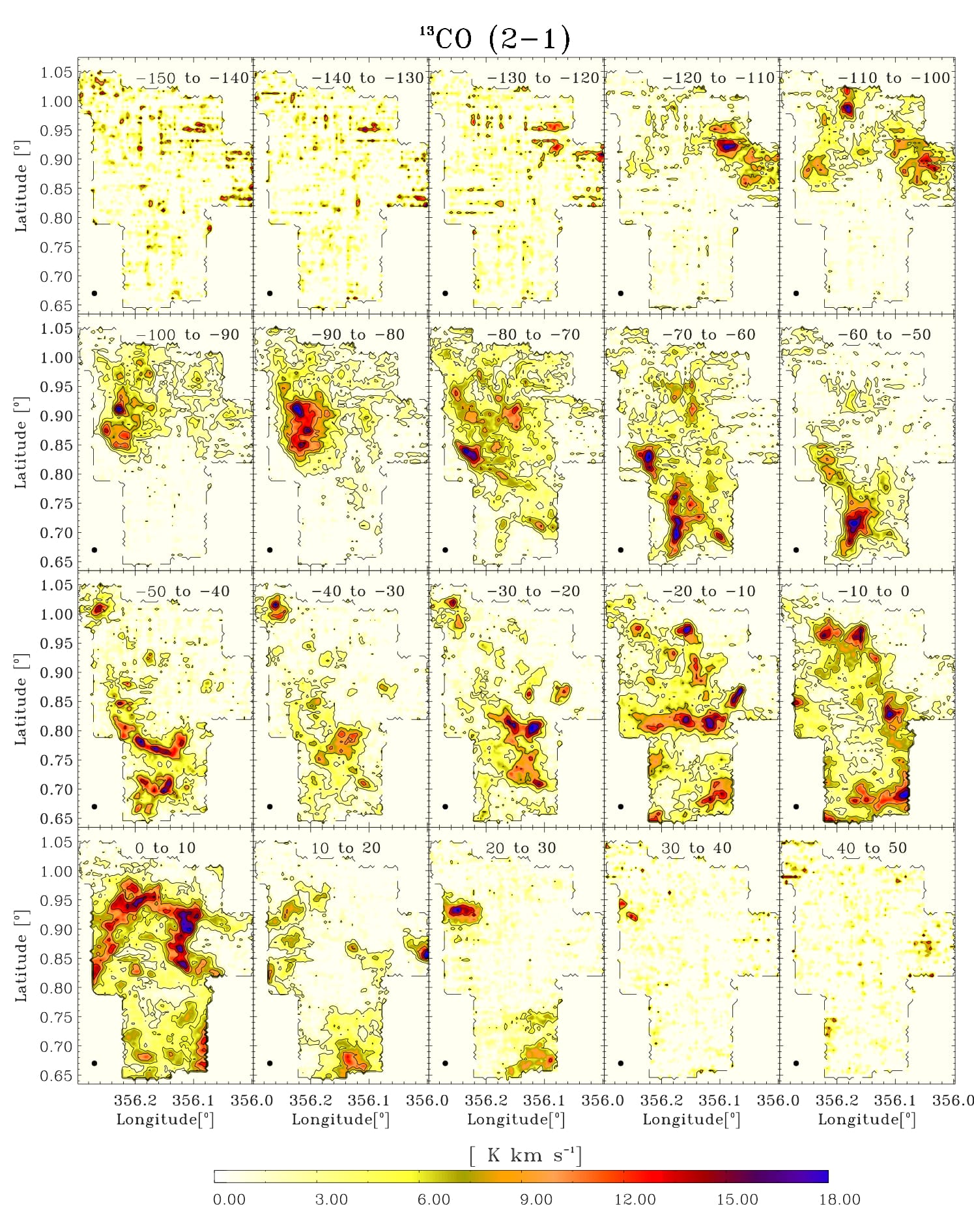
Figure 13: Integrated brightness temperature of the M$-3.8+0.9$ molecular cloud in ¹³CO $(2-1)$ in velocity intervals of $10$  km s^-1.

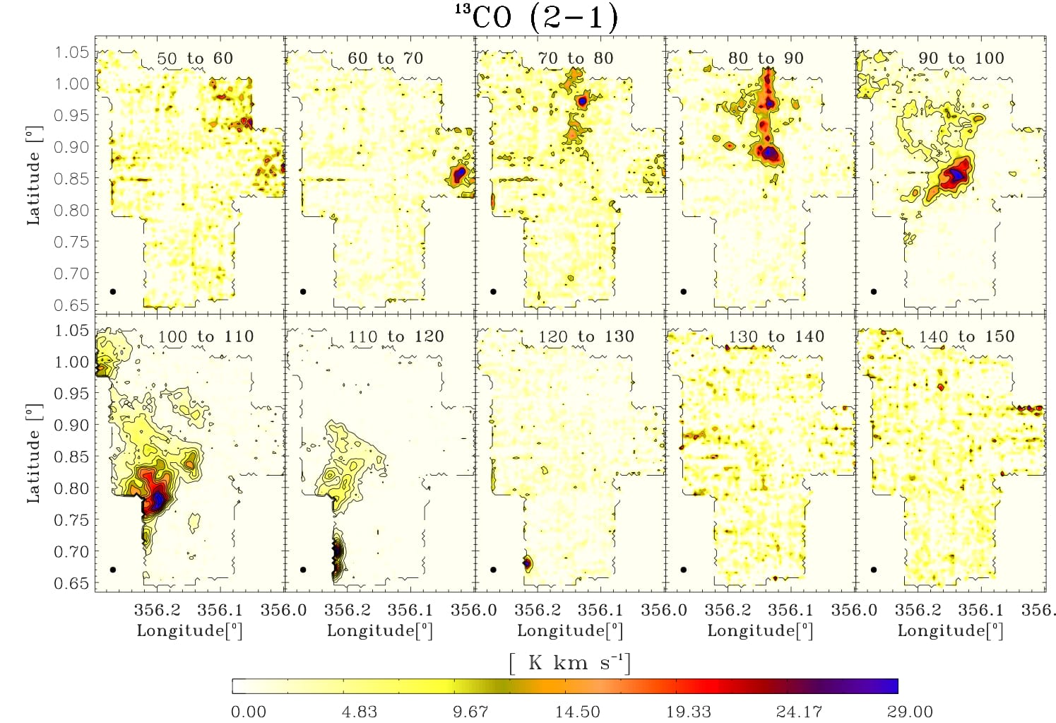
Figure 14: Integrated brightness temperature of the M$-3.8+0.9$ molecular cloud in ¹³CO $(2-1)$ in velocity intervals of $10$  km s^-1, continuation.

Figs. 2 and 3 show: I) the integrated brightness temperature maps of HCN and ¹³CO $(2-1)$, for the observed region of M$-3.8+0.9$, in the velocity range from $v_{\rm LSR}=-140$ to$v_{\rm LSR}=-20$  km s^-1, II) the longitude-velocity map integrated over the whole observed latitude range, and III) the latitude-velocity map integrated in the whole observed longitude range. Fig. 4 and 5 show the integrated brightness temperature of the molecular emission in velocity intervals of 10 km s^-1 in HCN, and in Fig. 13 and 14 we show the ¹³CO $(2-1)$ emission. The M$-3.8+0.9$ cloud has a narrow line width emission at positive velocities ($\sim$120  km s^-1) at $(l,b)\sim(356{{}^{\circ}}.25,0{{}^{\circ}}.70)$, which can be seen in the HCN emission (Fig. 5). Its position coincides with that of an ultra compact H II region (Caswell & Haynes 1987), but this source has a radial velocity of $113$  km s^-1, and therefore is not associated to the foot point as noted by Torii et al. (2010a). Therefore this source will not be further discussed in this work. This source was only partially covered by the ¹³CO observation. There are also several molecular clouds showing positive velocities in the ¹³CO emission (Fig. 14). The emission at $\sim 70-90$  km s^-1could be associated to the far-3 kpc arm (Dame & Thaddeus 2008) and the emission at $90-130$  km s^-1could be associated to the 135  km s^-1arm (Bania 1980)), as noted by Riquelme et al. (2010b), which are not associated with the loops 1 and 2, and they will not be discussed in this work.

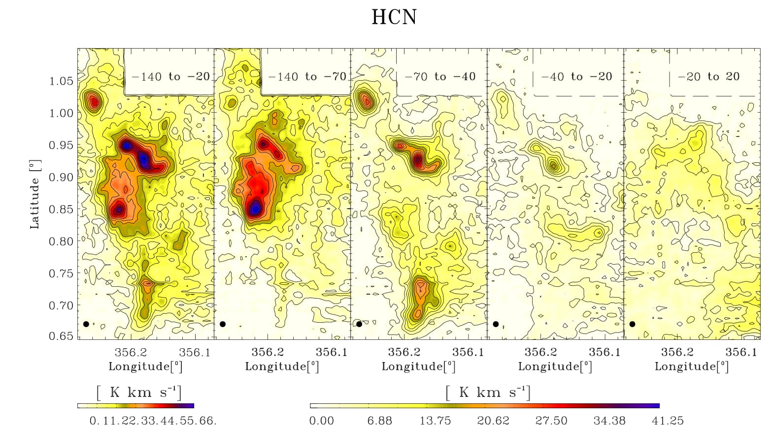
Figure 23: Velocity integrated emission in HCN. From left to right: velocity range from -140 to 20  km s^-1(the complete velocity range covered by the GMLs); velocity range from -140 to -70  km s^-1; -70 to -40  km s^-1, -40 to -20 km s^-1and -20 to 20  km s^-1

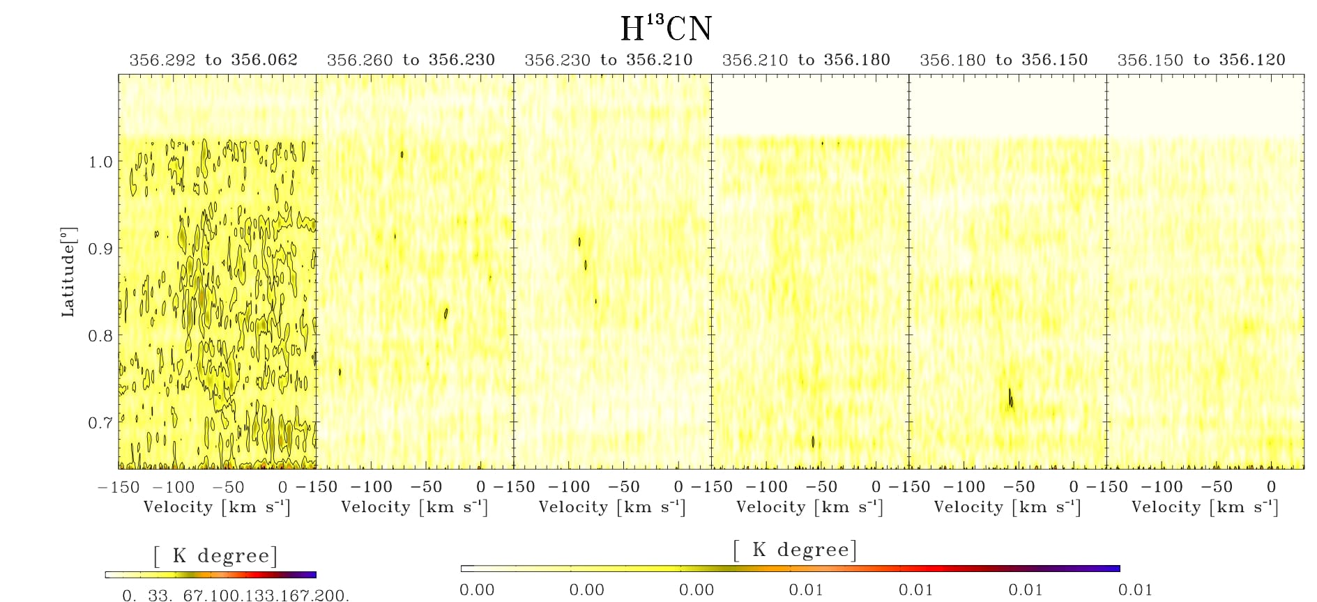
Figure 33: Latitude-velocity maps of the H¹³CN emission integrated in the complete longitude range from 356^∘.29165 to 356^∘.06249 (Left), and in longitude steps of 108” (second panel to the right).

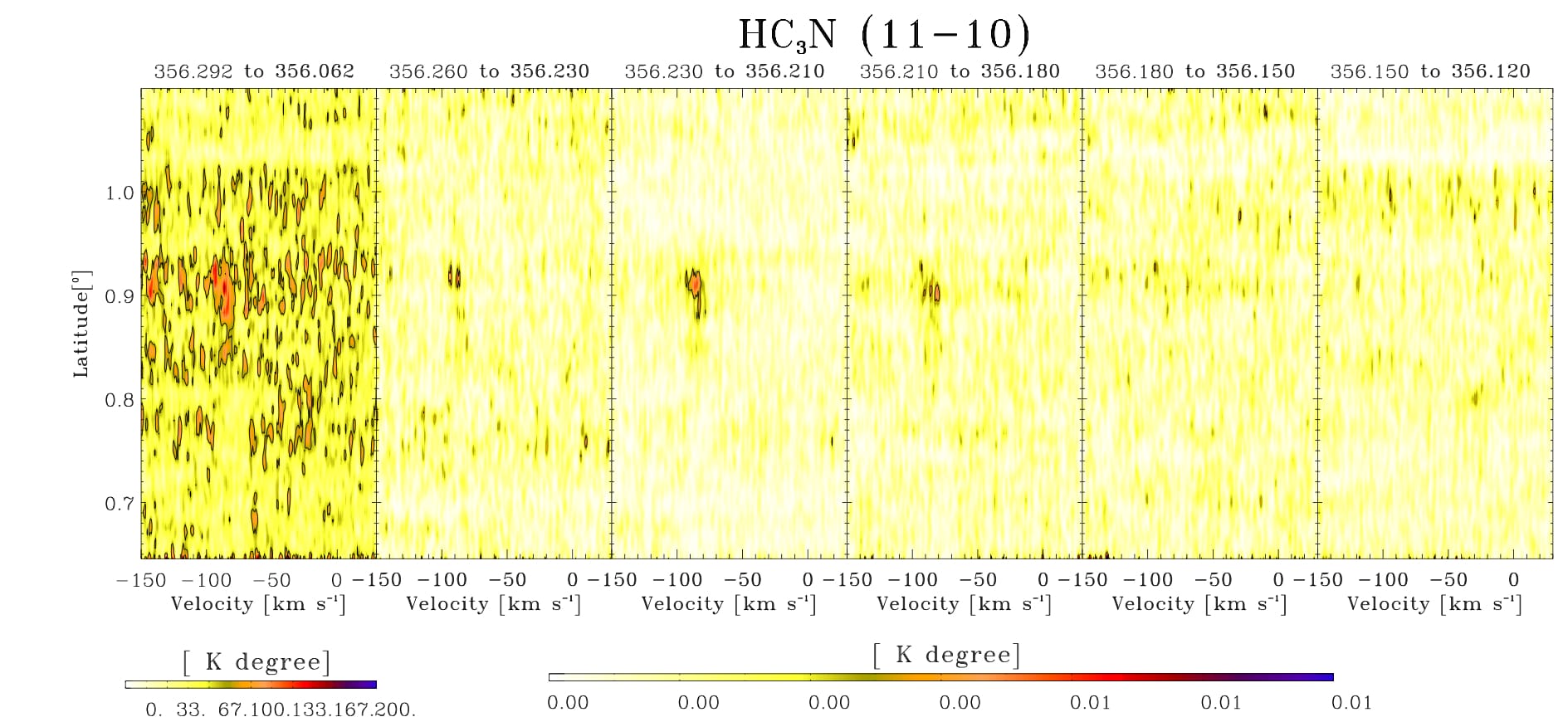
Figure 45: Latitude-velocity maps of the HC₃N (11-10) emission integrated in the complete longitude range from 356^∘.29165 to 356^∘.06249 (Left), and in longitude steps of 108” (second panel to the right).

Figs. 4 and 13 show the presence of a velocity gradient from higher to lower velocities in the north-western to the south-eastern direction. Four main velocity components were identified: from $-140$ to $-70$  km s^-1, from $-70$ to $-40$  km s^-1, from $-40$ to $-20$  km s^-1, and from $-20$ to $20$  km s^-1. In Fig. 23 to 32 we show the integrated intensities maps between $-140$  km s^-1and $-20$  km s^-1as well as the integrated intensities maps in the four velocity ranges for all the detected transitions listed in Table 2. In these velocity ranges, six main molecular complexes are identified, indicated by green boxes in Fig. 6 on the HCN maps. These complexes were identified by visual inspection and may be spatially correlated if the M$-3.8+0.9$ cloud has a velocity gradient of 2 km ^-1 pc^-1. For an easy comparison, the ¹³CO emission is also plotted in this figure. The velocity structure is also shown in the latitude-velocity domain integrated in longitude steps of 108” (from Fig. 33 to Fig. 45). In those figures we can see the two “U-shapes” identified by Torii et al. (2010b) (see Section 5.4).

3.2 Complex 3

In the velocity range from $-140$ to $-70$  km s^-1, the most prominent feature is the Complex 3, which shows an elongated structure perpendicular to the Galactic plane with an abrupt sharp intensity decrease towards the eastern edge. This complex also contains two intensity peak which are detected in most of the molecules (see the Figs. in Appendix C) at $(l,b)=(356{{}^{\circ}}.22,0{{}^{\circ}}.91)$ and $(l,b)=(356{{}^{\circ}}.21,0{{}^{\circ}}.84)$. The ¹³CO, HC₃N, N₂H⁺, and SO molecular emissions have the intensity peak in the north, in contrast with the HCN , HCO⁺, and CS emissions which have the intensity peak in the south. Some molecules only appear in the north (e.g., HNCO, N₂H⁺, SO, and HC₃N).

3.3 Complexes 1, 2, 4, 5 and 6

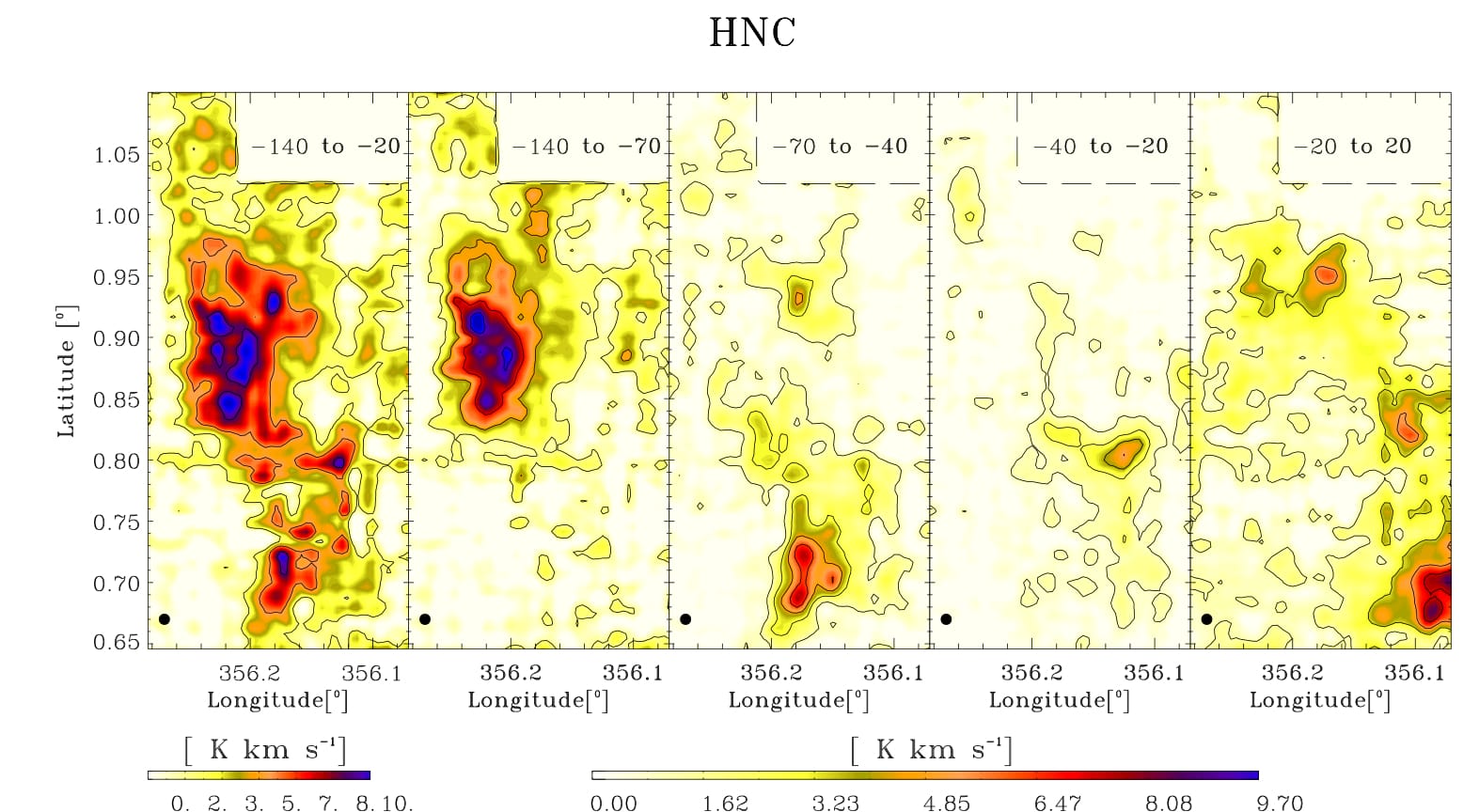
Figure 25: Velocity integrated emission in HNC. From left to right: velocity range from -140 to 20  km s^-1(the complete velocity range covered by the GMLs); velocity range from -140 to -70  km s^-1; -70 to -40  km s^-1, -40 to -20 km s^-1and -20 to 20  km s^-1

In the velocity range from $-70$ to $-40$  km s^-1, the Complexes 1, 2, 4 and 6 can be identified. Complex 1 has a very large line-width ($-110$ to 0  km s^-1). It is also strong in HCN emission, while in HCO⁺ emission the intensity is weaker but still cover the same velocity range. In the other molecules, the emission shows two kinematic components with the intensity peak at $\sim-40$  km s^-1. This complex is very prominent in the HCN, HCO⁺, CS, HNC, and CH₃OH emission (see from Fig. 23 to 32). Although the Complex 2 is not visible in all the detected molecules, it is the region which presents the largest line width in the M$-3.8+0.9$ molecular cloud, as can be seen in the Appendix C which is consistent with previous works (see, Torii et al. 2010b, a). The Complex 4 looks like connecting the Complex 3 and 6. This complex is very prominent in ¹³CO, CS, HCO⁺, HCN, and HNC. It is remarkable that Complex 6 also shows an elongated structure perpendicular to the Galactic plane similar to that observed for Complex 3. This complex also shows an abrupt sharp intensity decrease towards the eastern edge. In the velocity range from $-40$ to $-20$  km s^-1, we can see the Complex 5 which is an elongated feature, parallel to the Galactic plane. In the last velocity range, from $-20$ to $20$  km s^-1, the emission shows a shell-like structure which appears over the complete molecular cloud and is clearly seen in the ¹³CO, HCO⁺ and HNC maps (Figs. 6, 24 and 25). As can be seen in the channel maps of ¹³CO plots (Fig. 13, this feature is indeed narrower in velocity, from -10 to 10  km s^-1. This emission could be associated to local gas along the line of sight and since it is probably not associated to the GMLs, this feature will not be discussed in this work.

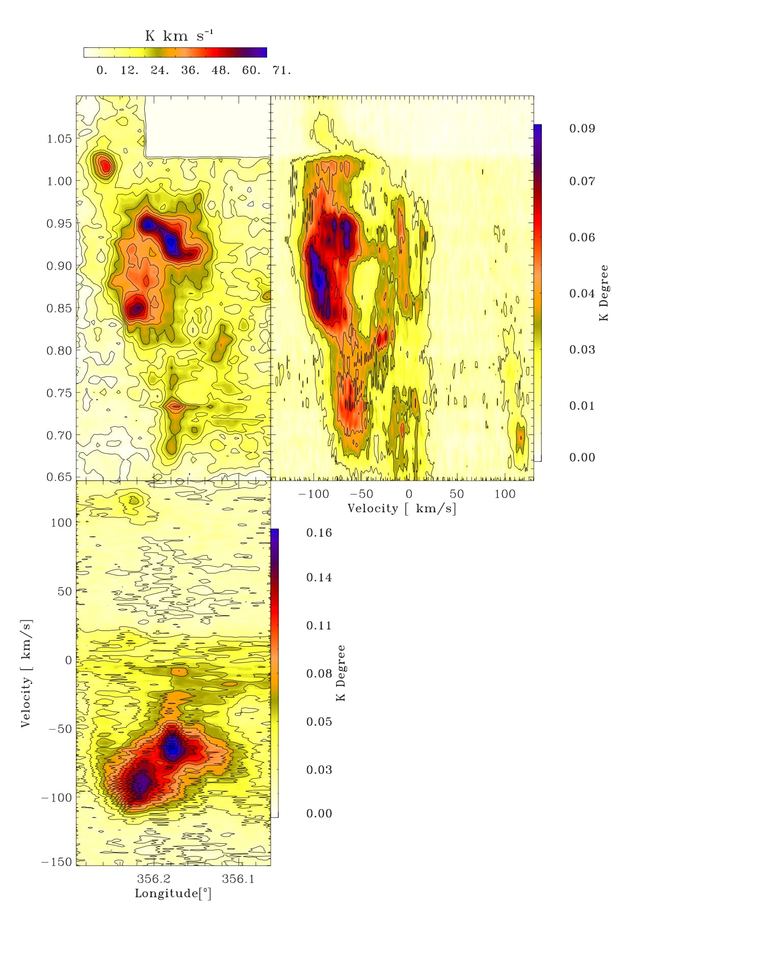
Figure 2: HCN $(1-0)$ emission of the M$-3.8+0.9$ cloud: Left. Integrated brightness temperature map in the velocity range from $-140$ to $-20$ km s^-1. Right. Latitude-velocity plot integrated over the whole longitude range (from $l=356.29{{}^{\circ}}$ to $356.06{{}^{\circ}}$). Bottom. Longitude-velocity plot integrated over the whole latitude range (from $b=0.64{{}^{\circ}}$ to $b=1.10$^∘).

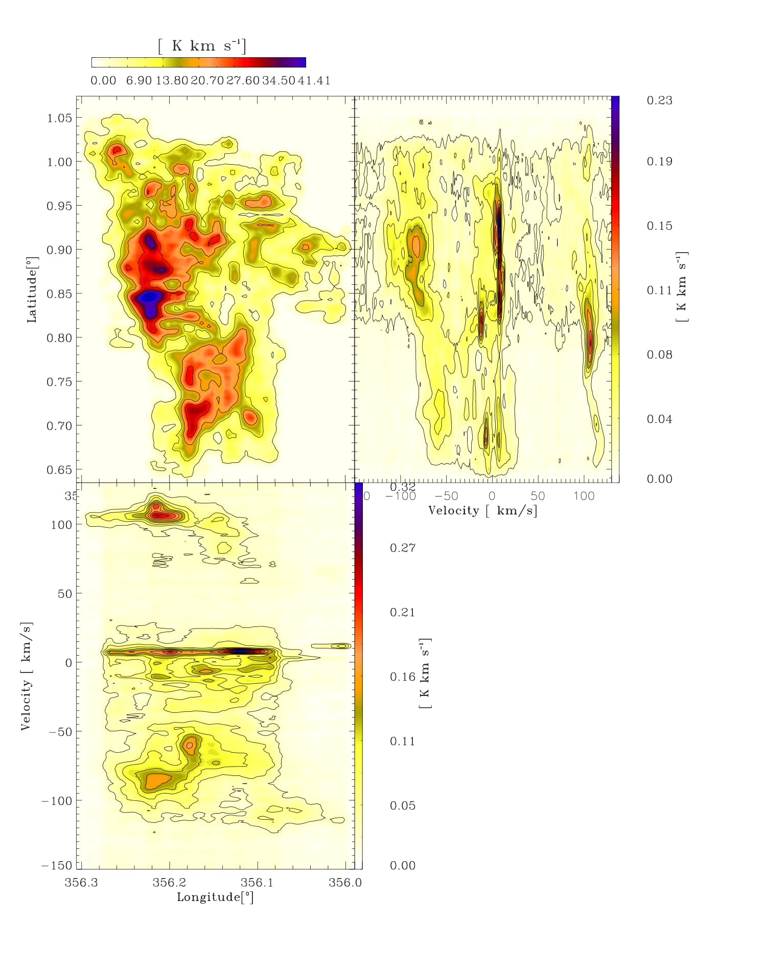
Figure 3: ¹³CO (2-1) emission of the M$-3.8+0.9$ cloud: Left. Integrated brightness temperature map in the velocity range from $-140$ to $-20$ km s^-1. The dashed lines show the mapped region. Right. Latitude-velocity plot integrated over the whole longitude range (from $l=356{{}^{\circ}}$ to $356{{}^{\circ}}.294$). Bottom. Longitude-velocity plot integrated over the whole latitude range (from $b=0{{}^{\circ}}.6423$ to $b=1{{}^{\circ}}.051$)

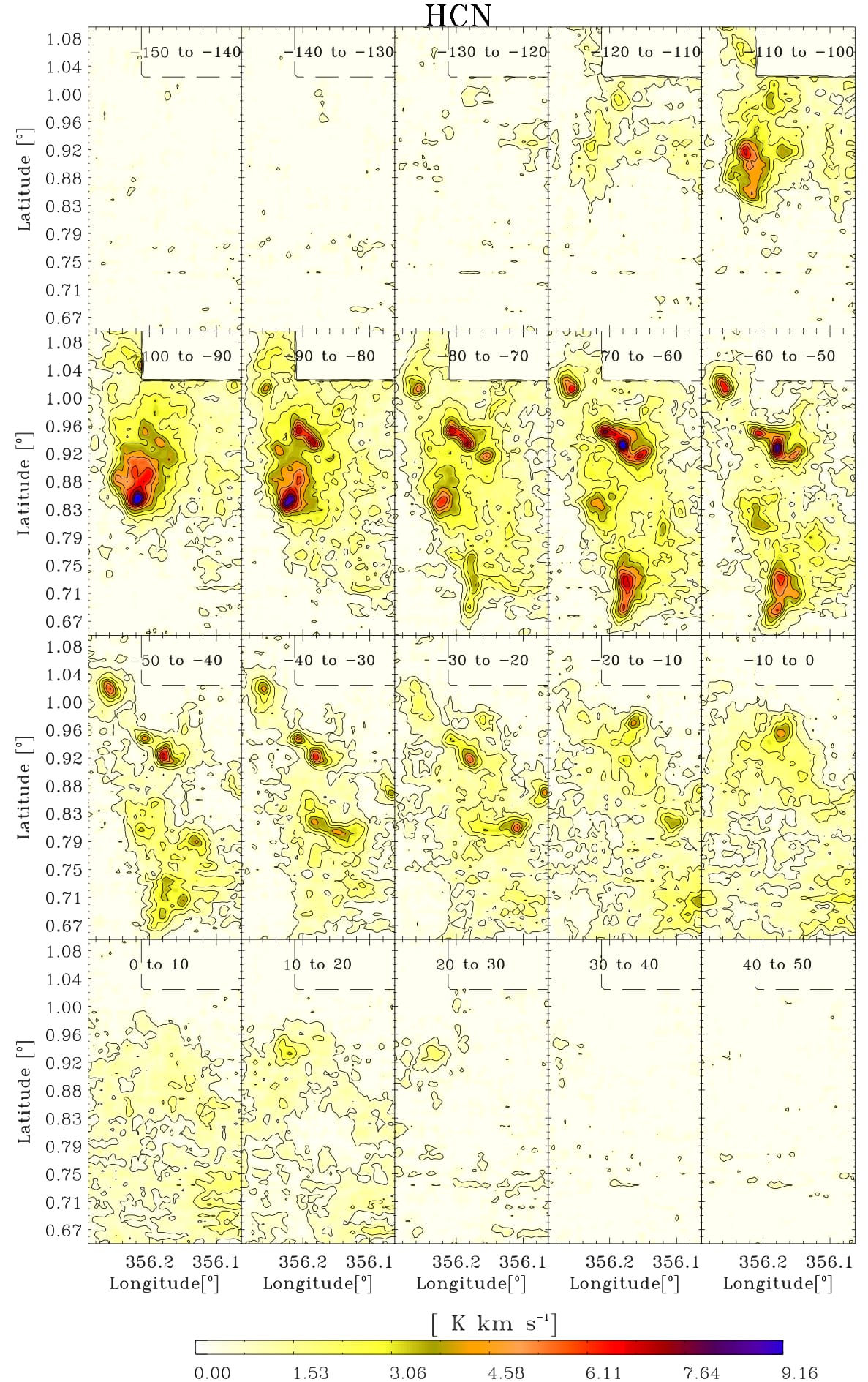
Figure 4: Integrated brightness temperature of the M$-3.8+0.9$ molecular cloud in HCN $(1-0)$ in velocity intervals of $10$  km s^-1.

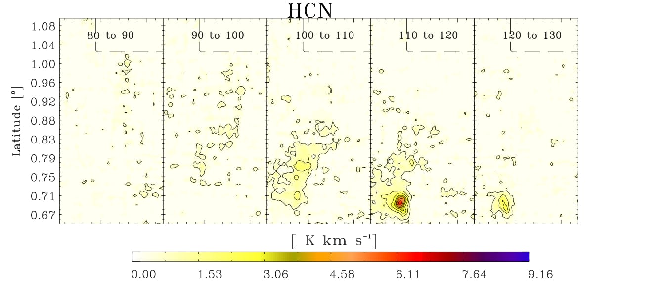
Figure 5: Integrated brightness temperature of the M$-3.8+0.9$ molecular cloud in HCN $(1-0)$ in velocity intervals of $10$  km s^-1.

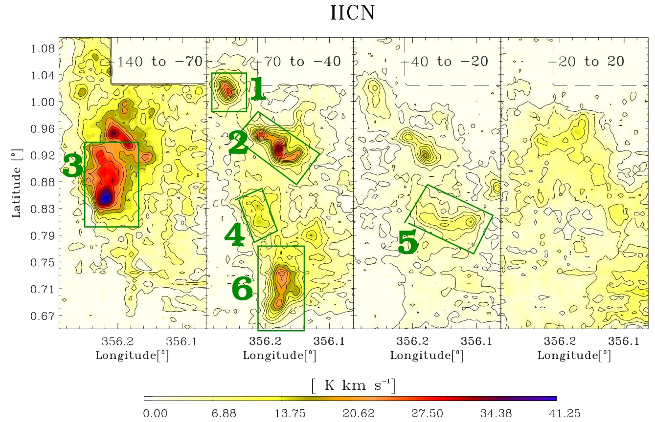
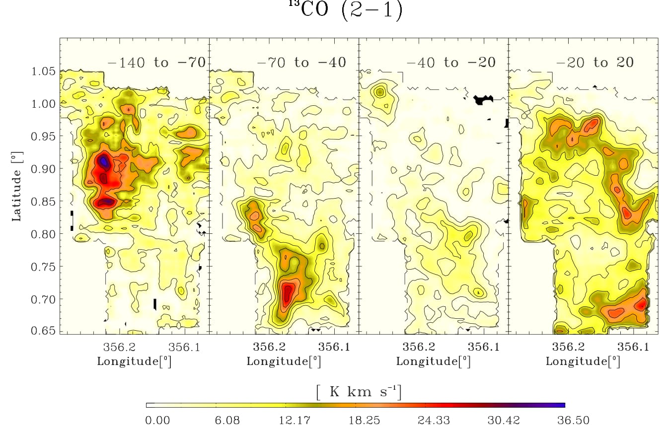
Figure 6: Position of the six molecular complexes discussed in the text. The green boxes show the complexes discussed in the text.

4 Analysis

4.1 ¹³CO (2-1) emission. H₂ Column density estimate

Since the ¹³CO emission is optically thin (see optical depth estimations for CO in (Torii et al. 2010a)) and the critical density is relatively low ($n_{\rm crit}\sim 10^{4}$ cm^-3), this molecule is a good tracer of the total H₂ column density using a proper conversion factor ($N({\rm H_{2}})=N({\rm{}^{13}CO})\times[{\rm{}^{13}CO/H_{2}}]$). Since we only have one transition, we assume local thermodynamical equilibrium (LTE) at a excitation temperature ($T_{\rm{ex}}$) of 10 K to derive the column density, N:

$$N=\frac{8\pi k\nu^{2}Q(T_{\rm ex})}{c^{3}A_{ij}g_{u}h}\exp{\Bigg{(}\frac{E_{u}}{kT_{\rm ex}}\Bigg{)}}\frac{1}{\Big{(}1-\frac{J(T_{\rm bg})}{J(T_{{\rm ex}})}\Big{)}}\int T_{b}dv$$ (1)

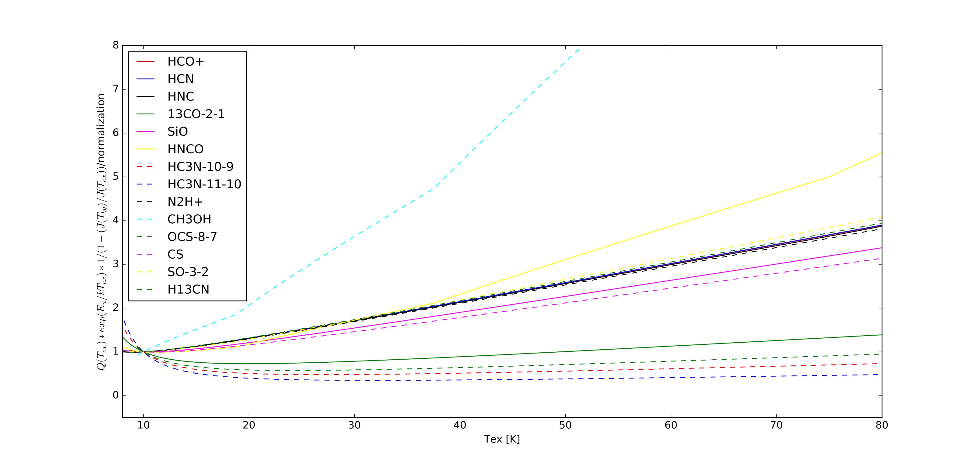
Figure 15: Variation of column density with excitation temperature, T_ex. The y-axis shows the T_ex-dependent parameters in Eq. 1 normalized to T${}_{\rm ex}=10$ K. For ¹³CO (2-1), we can see that the difference between the assumption of T${}_{\rm ex}=10$ K and 40 K (which is the temperature estimated by the detailed work of Torii et al. (2010a) is $\sim$ 10%. Most of the species in the 3-mm molecular transitions show a factor $<2$ if we increase the T_ex at 40 K, with the exception of CH₃OH which is highly dependent of the T_ex; and OCS and HC₃N.

where $k$ is the Boltzmann constant, $\nu$ the frequency of the transition, $h$ the Planck constant, $Q(T)$ the partition function at the assumed excitation temperature, $g_{u}$ the upper state degeneracy, $A_{ij}$ the Einstein coefficient, $E_{u}$ the energy of the upper state, and $J(T)=\frac{h\nu}{k}\Big{(}\frac{1}{(\exp((h\nu)/(kT))-1}\Big{)}$ is the source function at a temperature T. The molecular parameters were taken from the Cologne Database for Molecular Spectroscopy (CDMS) catalog (Müller et al. 2005, 2001), and T${}_{\rm{bg}}=2.73$ K is the cosmic background radiation temperature. If we use the T${}_{\rm{ex}}=40$ K as derived by the multi-J transition study of ¹²CO by Torii et al. (2010a), the N(¹³CO) increase by less than 10% (see Fig. 15). Thus, we decided to use 10 K which is consistent with our estimations in Riquelme et al. (2013) for CS, and with the discussion in Section 5.1.

For our calculations, we assume an abundance ratio CO/H₂ of 10^-4 (Frerking et al. 1982). This abundance ratio was also used by Rodríguez-Fernández et al. (2001), Dahmen et al. (1998) and Hüttemeister et al. (1998) for their large scale studies of the GC, which cover the complete CMZ and the Bania’s clump2. As noted by Hüttemeister et al. (1998), Farquhar et al. (1994) showed that this ratio is stable against a possibly enhanced cosmic ray flux to the GC. Riquelme et al. (2010a) derived a high ¹²C/¹³C isotopic value ($34-73$) in several positions in this molecular cloud which is higher than the typical values (20-25) found in the GC region (see, e.g., Langer & Penzias 1990; Wilson & Matteucci 1992). Therefore, the value of 53 was used, corresponding to the typical value found in the 4 kpc molecular ring (Wilson & Rood 1994), which was also used by Torii et al. (2010a), Kudo et al. (2011) and Riquelme et al. (2013) in the GMLs regions. This translates into a $\mathrm{[^{13}CO/H_{2}]}$ conversion factor of $1.9\times 10^{-6}$.

4.2 Comparison of the emission between different molecules

To compare and quantify the differences and similarities between the emission distribution throughout the M$-3.8+0.9$ molecular cloud in the different detected molecules, we perform a principal component analysis and we derive the fractional abundances in selected positions.

4.2.1 Principal component analysis

A principal component analysis (PCA, see, e.g, Heyer & Schloerb 1997; Shlens 2014; Ungerechts et al. 1997; Lo et al. 2009; Jones et al. 2012) was performed using the most intense molecular lines in Table 2, namely ¹³CO, HCN, HCO⁺, HNC, CH₃OH, and CS. As mentioned in Section 2.1, the Mopra beam varies from $33\pm 3$” at 115 GHz and $36\pm 3$” from $86-100$ GHz. Then, the beams sizes for the molecules used in the PCA analysis are identical within the uncertainties. The resolution of the pixel in all data cubes is 15”. The ¹³CO $(2-1)$ data was converted to Galactic coordinates using standards class routines using one of the Mopra datacube (HCN) as a pattern, imposing the pixel size of 15”. Therefore, all data cube used in the PCA have a uniform spatial resolution. To implement the method, a python script with the PCA module is used in a similar way as Jones et al. (2012), using a covariance matrix method. Because the PCA analysis works with normalized data, we only can compare data with a good signal-to-noise ratio. Since the spectroscopic parameters from the different molecules and ¹³CO, as well as the critical densities are different, it is possible that the different molecules are not tracing the same gas. We used the integrated emission in the velocity range from $-140$ to $-20$ km s^-1, which covers the complete velocity range corresponding to the GC region since the emission from $-20$ to $20$  km s^-1correspond to local gas in the line of sight. The PCA is also restricted to an area defined using a mask in the HCN emission at a 14-$\sigma$ level (13.29 K  km s^-1). This threshold was chosen to include all the important features visible in the Figs. 23 to 32 and excluding the regions with low signal-to-noise ratio which can add spurious features in the PCA.

The PCA shows that the emission distribution of all the molecular lines studied are closely related. The first three principal components describe the 94, 2, and 1.5 per cent of the variance in the data. Fig. 7 shows the results of the PCA. The color scale indicates the correlation between the molecules. A positive value indicates that the emission from these molecules are correlated and the negative values show an anti-correlation. The first principal component axis in Fig. 8 shows that all 6 molecules are positively correlated. The PCA1 image in Fig. 7 shows emission common to the six molecular lines with a large fraction of the variance (94 per cent) indicating that all molecular lines are similar distributed throughout the molecular cloud. The major features are the complex 2 and 3 which show the largest correlations in the cloud. The PCA2 image shows the major difference among the six remaining molecules. Despite the value of the variance is small (2%), these differences are still physically significant because the positive features follow very well the Complex 2 which is dominant in HCN and HCO⁺, and the negative features correspond to the north part of the complexes 3, 4, 5, and 6 where ¹³CO, HNC, CH₃OH, and, to to less extent the CS emission are enhanced. The PCA3 has only a minimum value of the variance (1.5 %) and shows smaller variations mainly between the ¹³CO and HNC emissions.

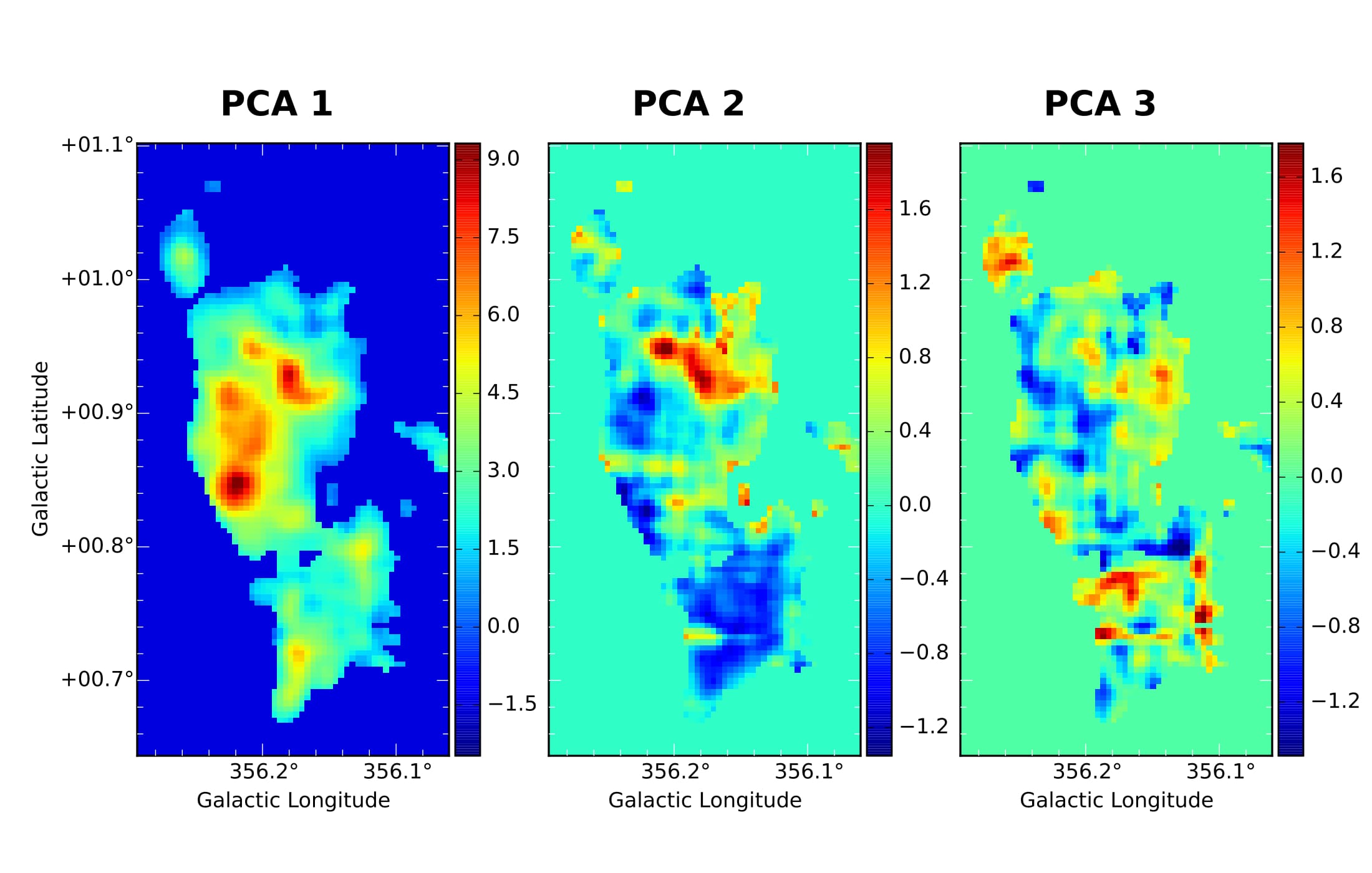
Figure 7: Images of the first three PC of the M$-3.8+0.9$ molecular cloud (see text in Section 4.2.1).

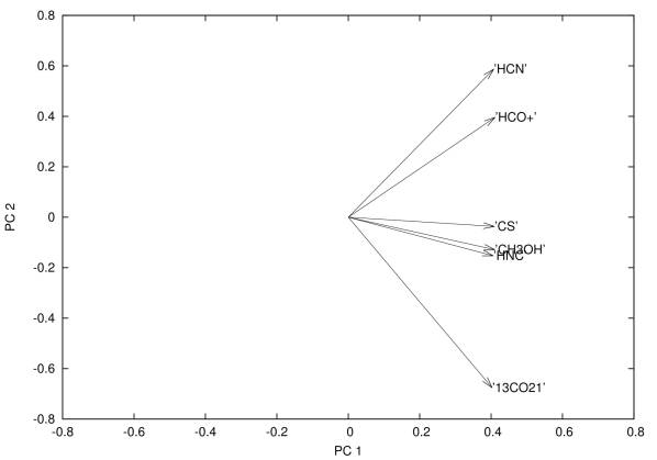
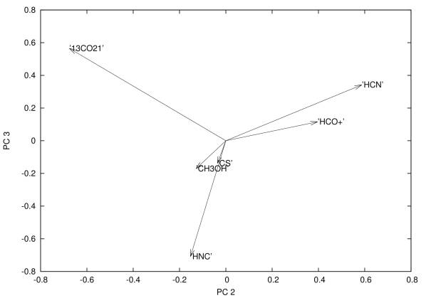
Figure 8: Plots of eigenvectors of the first three PC.

4.2.2 Spectra towards selected positions

Using the images of the different PCA previously discussed, we select 11 positions which have an intensity peak in the PCA1, which corresponds to the regions where the most intense molecules are correlated, and peaks in the PCA2 which corresponds to regions with the largest anti correlation between them. We selected at least one position per complex (complex 1 to 6 as defined in Section 3.1), then for example, the position chosen towards the complex 4 is not spotlighted in any of the PCA results. Because of the high correlation between the molecular transitions, this selection is equivalent to select the peaks in any of the 6 molecules considered in the PCA analysis. We obtain the integrated spectra in the boxes shown in Fig. 9 in all the detected molecules (Figs. 10 and 11). From those figures, we can see the complex velocity structure in the M$-3.8+0.9$ molecular cloud, with large velocity widths in all the selected regions. Most of the molecules show a similar line profile within each region, with the clear exception of HCN, which in some regions has the intensity peak at a very different velocity. A clear example is shown in positions 1.a, 2.a, 2.b, and 5.a, with the most extreme case in position 1.a where the profile of HCN differs completely from the one shown by the other molecules. The differences in the intensity peak of HCN could be explained by opacity effects since the N(HCN)/N(H¹³CN) ratio range from 6 to 21 which indicates that the HCN is optically thick. Position 3.b shows a characteristic shock profile (see e.g., Jiménez-Serra et al. 2009), with a prominent wing at the redshifted part of the spectra. The strong shock observed in this position produces a gas acceleration up to 50 km s^-1. As a good tracer of the column density, the ¹³CO spectra also clearly show the local gas in the line of sight as narrow emission at $\sim 0$ km s^-1, which is not seen in other molecules. This narrow emission is superposed to a broader one which corresponds to gas in the GC.

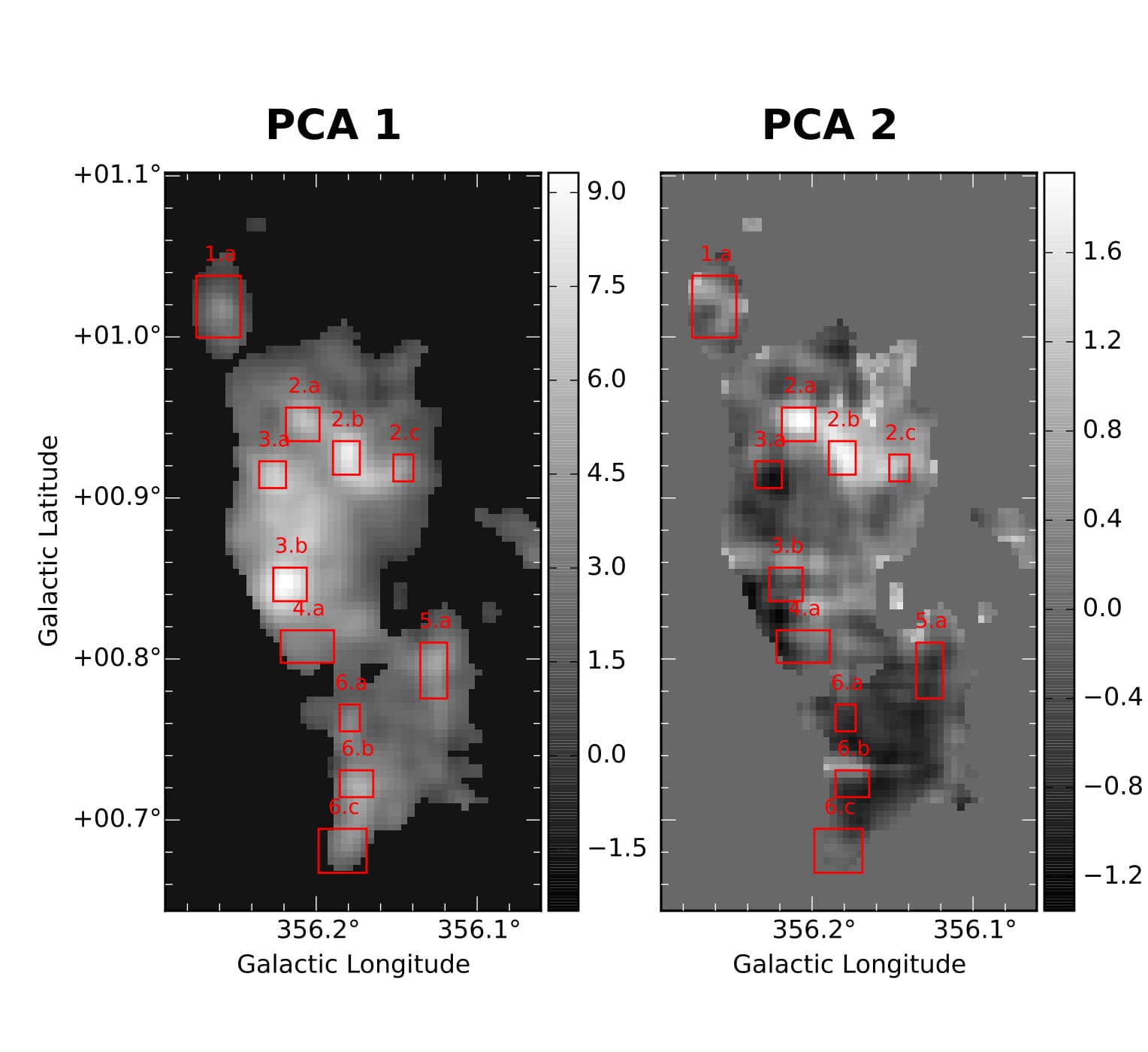
Figure 9: Selected regions to extract average spectra and to derive fractional abundances of the detected molecules.

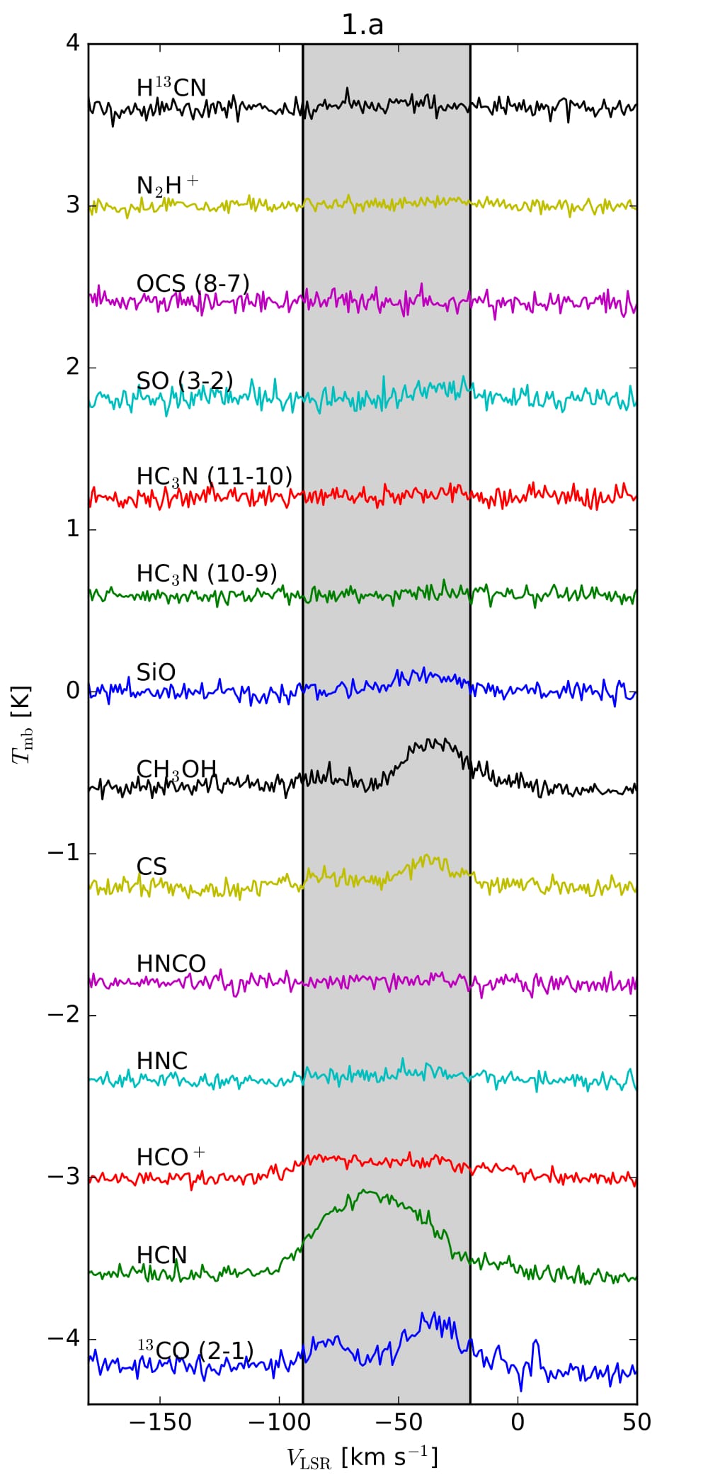
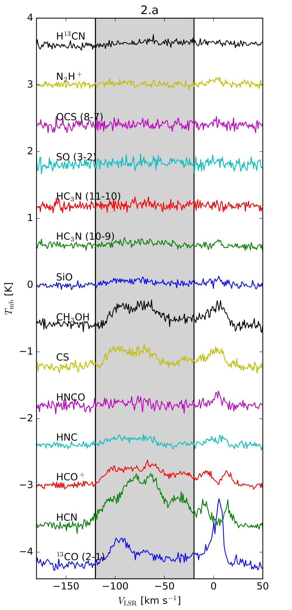
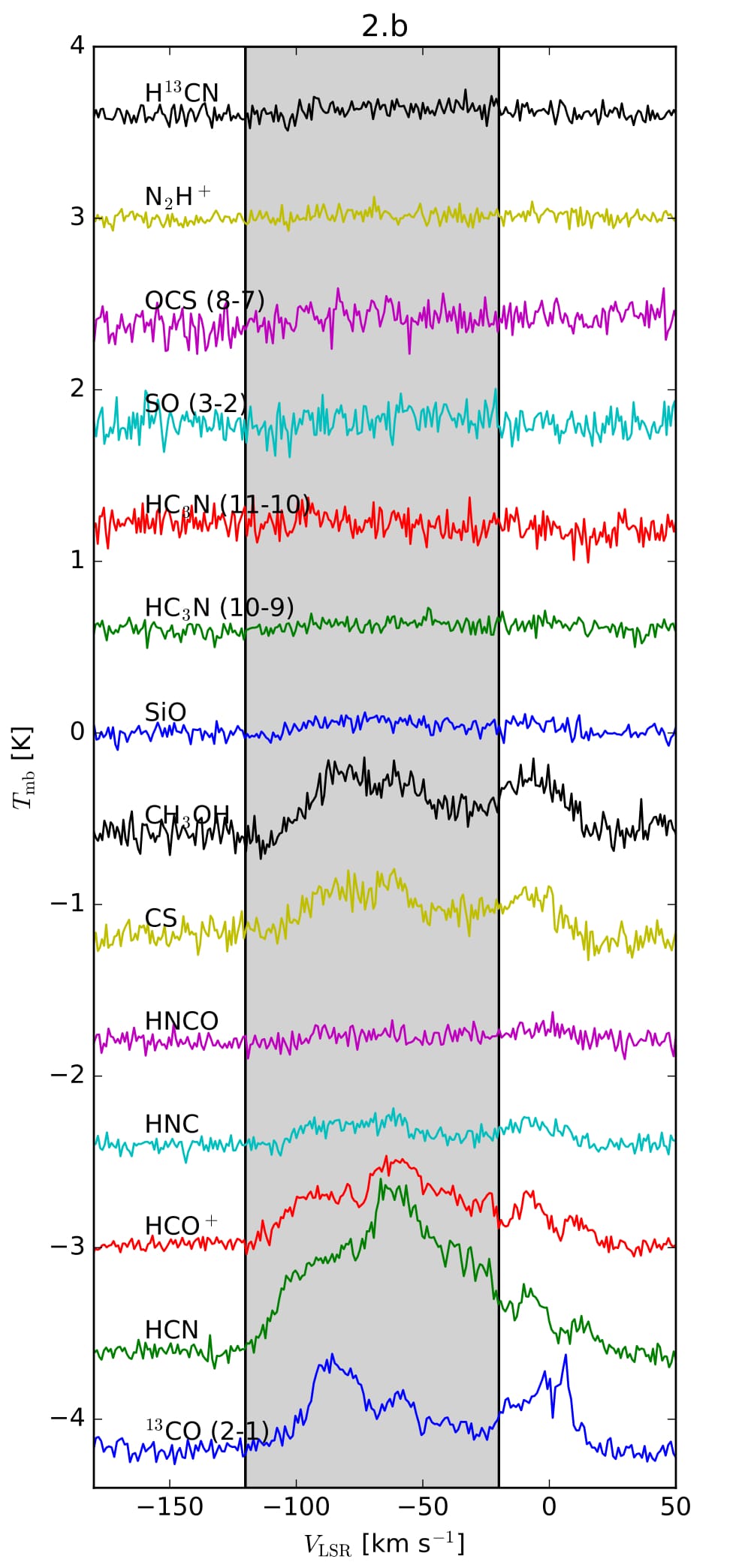
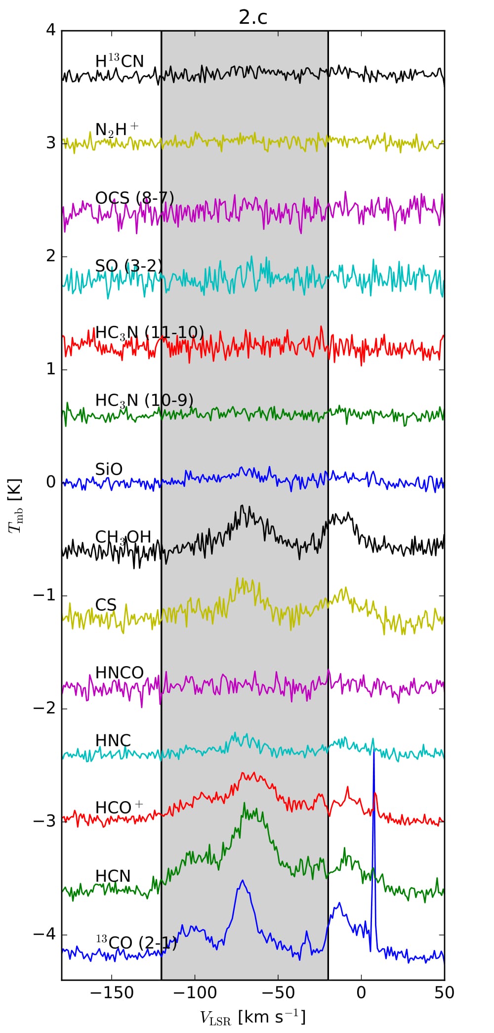
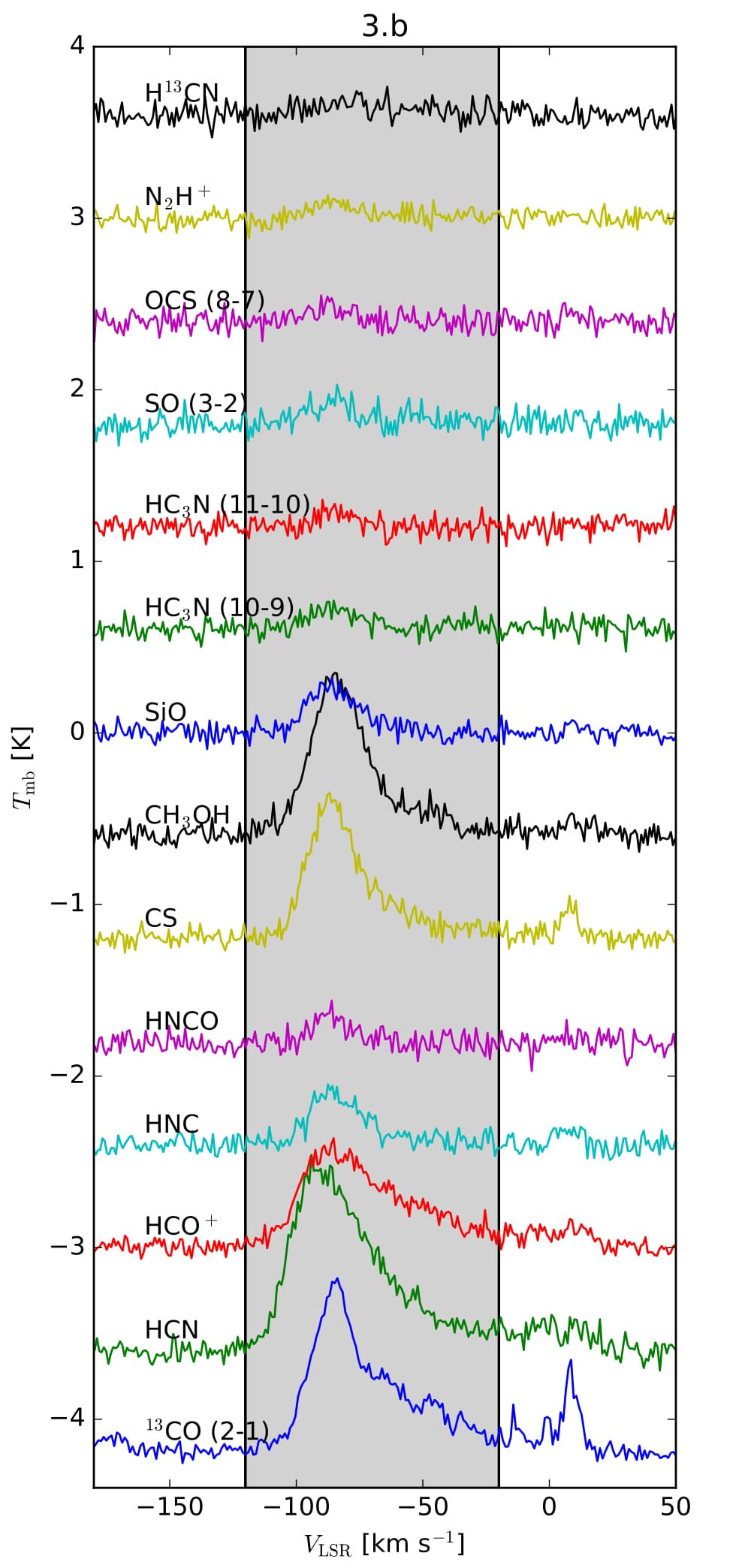
Figure 10: Average spectra for each box shown in Fig. 9. ¹³CO (2-1), HCO⁺, HCN, CH₃OH, CS spectra are scaled by a factor 0.5.

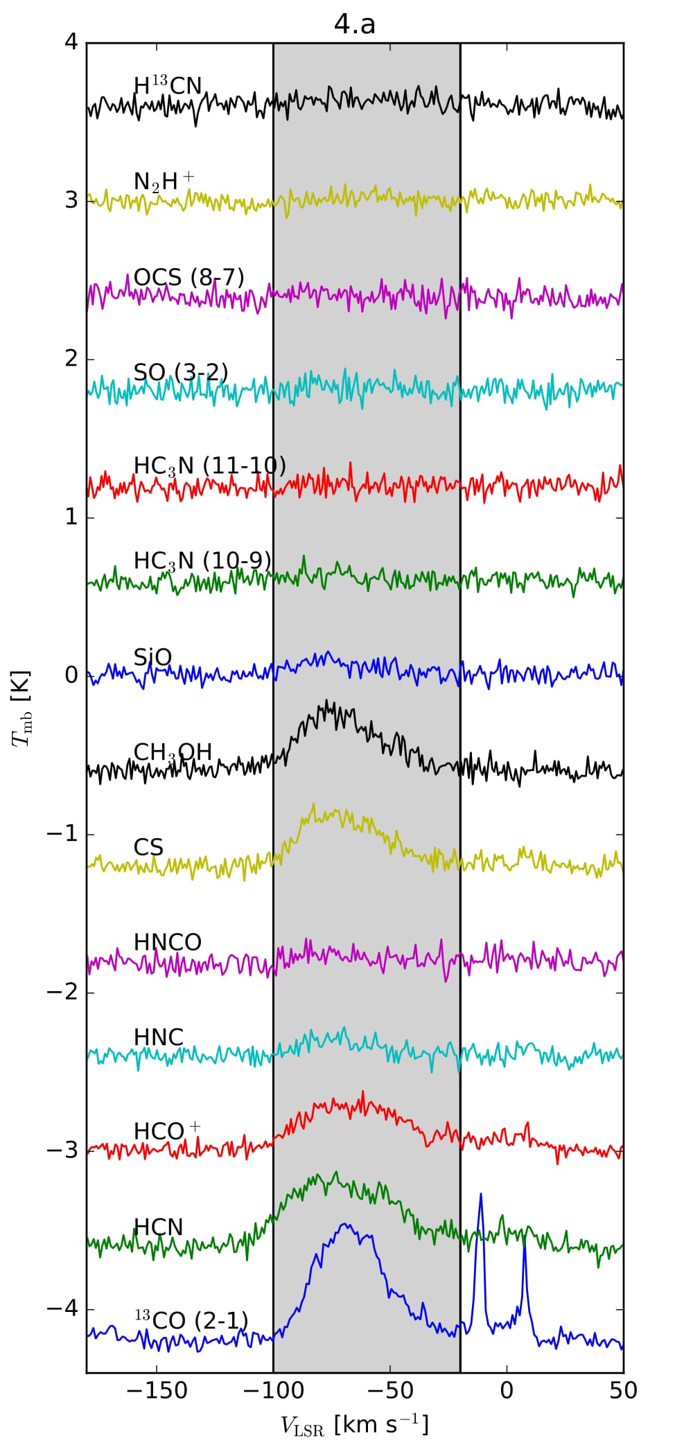
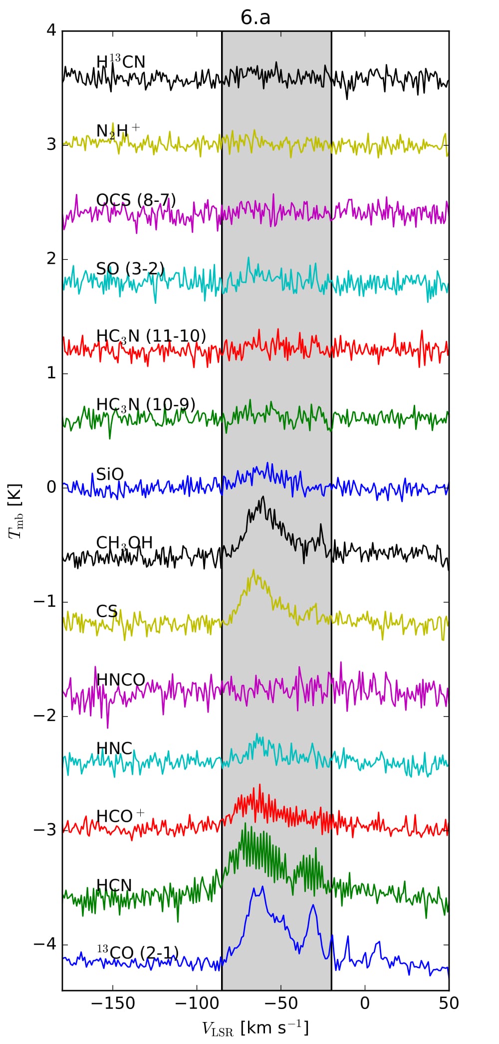
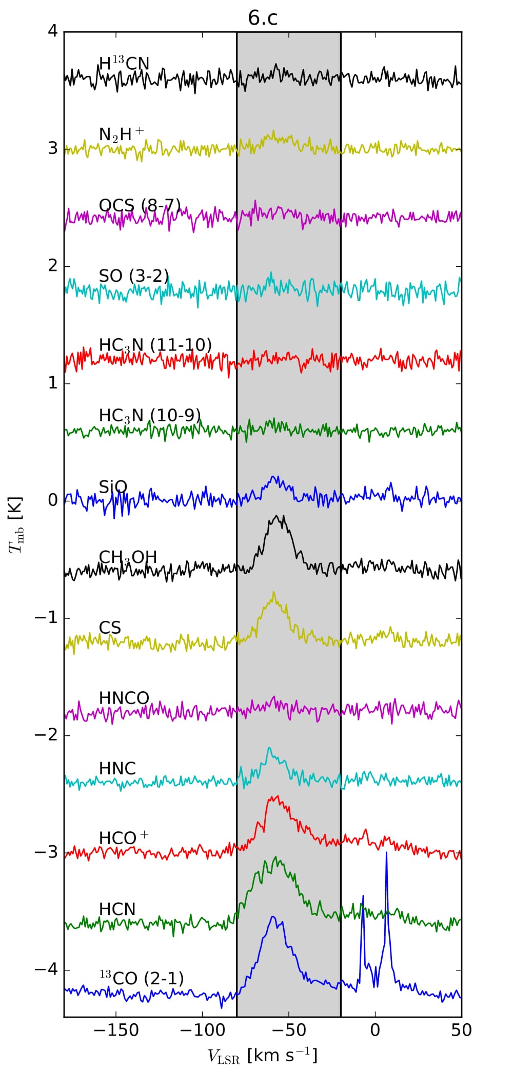
Figure 11: Average spectra for each box shown in Fig. 9.

4.2.3 Molecular abundances across the M$-3.8+0.9$ molecular cloud

The column density for all the detected molecules was derived as indicated in Section 3.2. Because we only have one transition for each molecule, we assume LTE at a $T_{\rm{ex}}=10$ K. If we assume a $T_{\rm{ex}}$ of, e.g., 24 K (Jones et al. 2012) column density varies a factor $\sim 1.5$ in most of the molecules considered here, as can be seen in Fig. 15 with the exception of CH₃OH which varies a factor of 2.5, and HC₃N (with a factor of 0.4). The molecular parameters are taken from the CDMS catalog for all the molecules with the exception of CH₃OH which are taken from the Jet Propulsion Laboratory (JPL) catalog (Pickett et al. 1998). The column density is derived for the 11 regions defined in Fig. 9 for the velocity range shown in the shadow rectangle in Fig. 10 and 11, and in the Table 6. The velocity range for each position was chosen to include all the emission for the M$-3.8+0.9$ cloud avoiding the possible contamination from local gas between $-20$ to $20$  km s^-1. Table 6 shows the results. HC₃N has two detected rotational transitions. This allows to better estimate the column density and rotational temperature using rotational diagrams (Goldsmith & Langer 1999). However, because the energy involved of both transitions are very close, the rotational temperature is poorly constrained, and only positions 3.a and 3.b have adequate signal-to-noise ratio in both transitions. Therefore, to derive the column density of HC₃N, we used only the (10-9) transition (which is the one with the better signal-to-noise ratio) assuming a temperature of 10 K like with the others species in this work.

To compare the emission from the different positions, we plot the fractional abundances ($X({\rm mol})=N({\rm mol})/N({\rm H_{2}})$, where mol corresponds to every detected molecule) normalized by the average value for each molecule. The fractional abundance is computed for the velocity range shown in Table 6, and Figs. 10 and 11. The plots show in the upper right corner, the average value and the standard deviation of the fractional abundance for each molecule, which is computed using only detected emission and not the upper limits. The error bars corresponds to the estimated 3-sigma uncertainties. Despite that the PCA analysis showed the large correlation between the most intense molecules across the M$-3.8+0.9$ molecular cloud, Fig. 12 shows that there are significant differences ($3-\sigma$) between the abundance of different molecules in the selected regions. The fractional abundances are shown in Table 4.

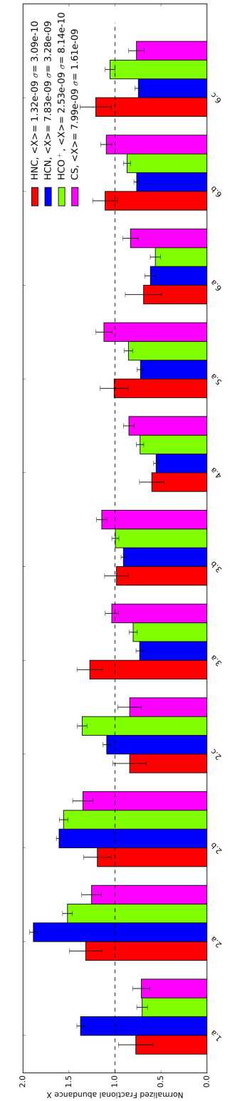
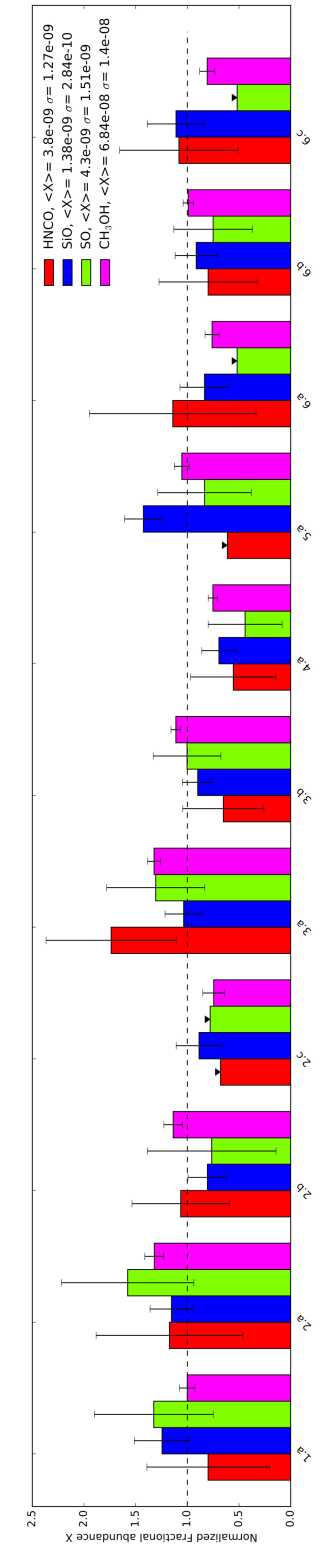
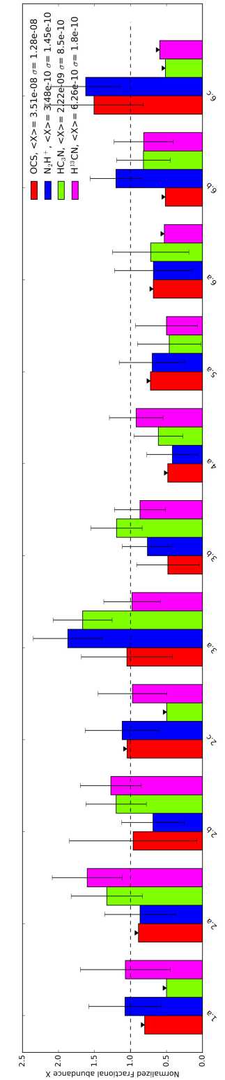
Figure 12: Molecular fractional abundance ($X({\rm mol})=N({\rm mol})/N({\rm H_{2}})$ normalized by the average value for each molecule. The label indicates the average value and the standard deviation for each molecule. We include all detected molecules shown in Table 2.

5 Discussion

5.1 Comparison between the molecular fractional abundances in the foot points and in the CMZ

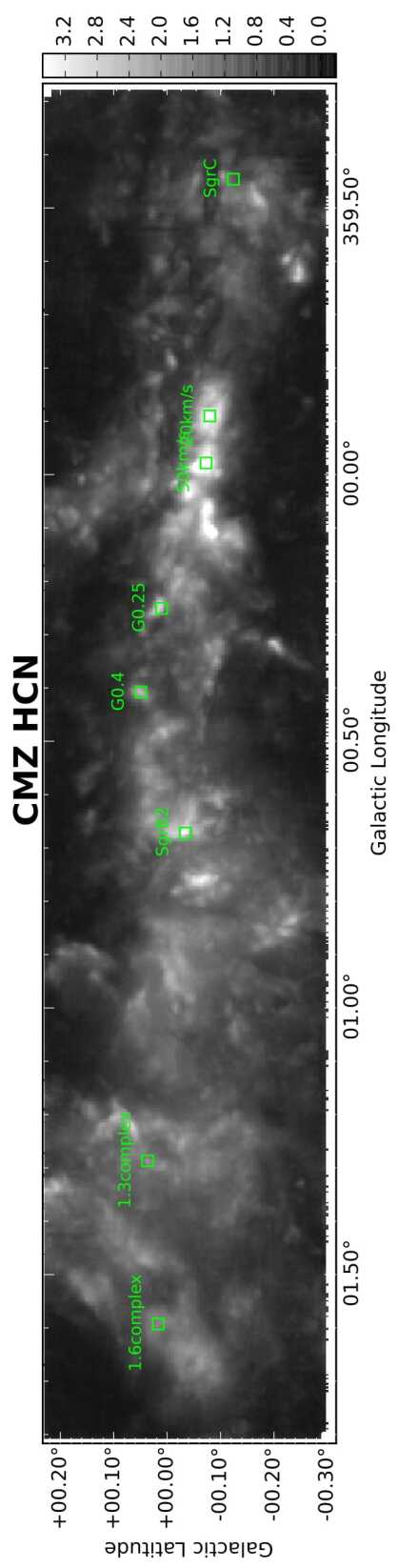
Figure 16: Selected regions for deriving the column densities for the detected molecules of this work overlaid on the peak brightness images of HCN from Jones et al. (2012)

The fractional abundances derived toward the foot points of the giant molecular loops are compared with those derived in the CMZ (Table 5). In order to obtain a set of fractional abundances values for the CMZ as homogeneous as the one presented in this work, we used the Mopra 3-mm data cubes from Jones et al. (2012) to derive the molecular column densities, and for estimating the H₂ column density, we used the “APEX CMZ SHFI-1 survey” ¹³CO (2-1) data cube from Ginsburg et al. (2016, available at http://doi.org/10.7910/DVN/27601). Since the ¹²C/¹³C isotopic value in the CMZ is 24 (Langer & Penzias 1990), we use a conversion factor [¹³CO/H₂] of $5\times 10^{-6}$]. We select representative clouds in the CMZ shown in Fig. 16. The regions were chosen to be of similar size in Fig. 9 $(75^{\prime\prime}x75^{\prime\prime})$. The column densities are derived assuming LTE with an excitation temperature of 10 K, using Eq. 1 for the optically thin emission; and for the optically thick emission (HCN, HCO⁺ and HNC), we use the equations in Jones et al. (2012), computing the optical depth along the velocity axis in the same way than in Jones et al. (2012). To assume that the ¹³CO emission is optically thin is a reasonable approximation as shown by Rodríguez-Fernández et al. (2001) from ¹³CO and C¹⁸O (J=1-0, 2-1) observations in many sources widespread in the CMZ and also in the clump 2 (Bania et al. 1986). We did not use the $T_{\rm ex}=24$ K because Jones et al. (2013) found that the excitation temperature for the lower rotational transitions of the molecules that they have 3-mm and 7-mm transitions observations available (SiO, HNCO, HC₃N, ¹³CS, HOCO⁺) was between 2 to 9 K, concluding that the excitation temperature have to be much lower than the kinetic temperature of 30 K. To derive the column density of CS, we use their optically thin isotopomer ¹³CS and a assumed ¹²C/¹³C isotopic value of 24. The SO emission from Jones et al. (2012) is not included because they observed a transition not detected by us, and because they only detected it clearly in Sgr B2. Using upper limit information is not meaningful because of the poor baselines of the spectra in the data cube. Table 5 also includes the fractional abundances derived in selected line-of-sights toward the CMZ from recent publications covering most of the species observed in this work. The ratio of the fractional abundances between the CMZ (Jones et al. (2012) data) and the GMLs range from a factor 1.1 up to 5.1 for the different molecules. The largest differences are found for HNCO, N₂H⁺, HNC. The smallest differences are found for SiO, with a factor of only $1.1$, which indicate similarities in the chemistry of this molecule in the CMZ and in the foot points. If we consider the same conversion factor between the CMZ and the M-3.8+0.9 cloud (see Section 4.1) the ratio of the fractional abundances between the CMZ and the GMLs is 0.5 up to 2 for the different molecules.

Table 4: Fractional abundances of all detected molecules in the selected regions defined in Fig. 9 integrated over the complete velocity range showed in Table 6.

Molecule	1.a	2.a	2.b	2.c	3.a	3.b	4.a	5.a	6.a	6.b	6.c
	[x 10-9]	[x 10-9]	[x 10-9]	[x 10-9]	[x 10-9]	[x 10-9]	[x 10-9]	[x 10-9]	[x 10-9]	[x 10-9]	[x 10-9]
H13CN	0.67 (0.13)	1.00 (0.10)	0.80 (0.09)	0.61 (0.10)	0.61 (0.08)	0.54 (0.07)	0.58 (0.08)	0.31 (0.09)	0.33	0.51 (0.09)	0.37
SiO	1.72 (0.12)	1.59 (0.10)	1.11 (0.09)	1.22 (0.10)	1.43 (0.08)	1.24 (0.07)	0.96 (0.08)	1.97 (0.08)	1.15 (0.11)	1.26 (0.09)	1.53 (0.13)
HNCO	3.04 (0.75)	4.46 (0.90)	4.04 (0.60)	2.58	6.60 (0.80)	2.48 (0.50)	2.11 (0.52)	2.33	4.33 (1.02)	3.03 (0.60)	4.11 (0.73)
HCN	10.77 (0.10)	14.79 (0.11)	12.59 (0.08)	8.54 (0.11)	5.73 (0.10)	7.12 (0.07)	4.33 (0.07)	5.66 (0.10)	4.82 (0.16)	5.99 (0.08)	5.84 (0.10)
HCO+	1.78 (0.05)	3.83 (0.04)	3.94 (0.04)	3.43 (0.04)	2.03 (0.04)	2.52 (0.03)	1.84 (0.03)	2.16 (0.04)	1.42 (0.05)	2.19 (0.03)	2.66 (0.04)
HNC	1.02 (0.08)	1.74 (0.08)	1.57 (0.07)	1.11 (0.08)	1.68 (0.06)	1.30 (0.06)	0.79 (0.06)	1.33 (0.07)	0.91 (0.09)	1.46 (0.06)	1.60 (0.08)
HC3N	1.11	2.94 (0.37)	2.66 (0.31)	1.10	3.69 (0.30)	2.64 (0.26)	1.36 (0.25)	1.02 (0.33)	1.59 (0.39)	1.82 (0.28)	1.14
N2H+	0.37 (0.06)	0.30 (0.06)	0.24 (0.05)	0.39 (0.06)	0.65 (0.06)	0.27 (0.04)	0.15 (0.04)	0.24 (0.05)	0.24 (0.06)	0.42 (0.04)	0.57 (0.06)
CH3OH	68.44 (1.70)	90.26 (2.09)	77.77 (2.05)	50.9 (2.42)	90.4 (1.44)	75.9 (1.08)	51.4 (1.05)	72.0 (1.63)	52.0 (1.55)	67.79 (1.13)	55.2 (1.68)
OCS	28.16	31.20	33.76 (10.3)	36.7	36.8 (7.39)	16.8 (5.07)	16.9	25.3	23.9	18.08	52.8 (8.02)
CS	5.71 (0.25)	10.04 (0.28)	10.79 (0.30)	6.72 (0.35)	8.27 (0.19)	9.15 (0.15)	6.78 (0.16)	8.96 (0.24)	6.65 (0.22)	8.75 (0.16)	6.13 (0.23)
SO	5.69 (0.83)	6.78 (0.92)	3.28 (0.89)	3.35	5.61 (0.68)	4.31 (0.47)	1.89 (0.51)	3.58 (0.65)	2.23	3.23 (0.55)	2.23

Table 5: Fractional abundances for the CMZ from previous works

Molecule	1.6 complexa	1.3 complexa	Sgr B2a	G0.4a	G0.25a	50km/sa	20km/sa	Sgr Ca
	(20,210)e	(40, 230)e	(20, 140)e	(-20,60)e	(5,100)e	(0,100)e	(-20, 80)e	(-80,-5)e
	[x 10-9]	[x 10-9]	[x 10-9]	[x 10-9]	[x 10-9]	[x 10-9]	[x 10-9]	[x 10-9]
H13CN	1.11 (0.06)	1.34 (0.03)	0.66 (0.02)	1.02 (0.03)	1.17 (0.02)	1.63 (0.01)	1.53 (0.02)	0.61 (0.03)
SiO	2.47 (0.08)	2.60 (0.04)	1.12 (0.02)	1.40 (0.03)	1.05 (0.02)	1.40 (0.01)	1.60 (0.03)	0.50 (0.05)
HNCO	41.13 (0.40)	10.39 (0.23)	26.32 (0.17)	21.12 (0.19)	14.32 (0.17)	10.52 (0.09)	17.62 (0.23)	3.62 (0.26)
HCN	14.92 (0.05)	17.18 (0.08)	¿10.34	13.27 (0.03)	15.95 (0.02)	¿23.19	22.30 (0.03)	8.22 (0.05)
HCO+	4.17 (0.04)	5.17 (0.03)	¿3.96	2.25 (0.01)	2.74 (0.02)	3.50 (0.01)	4.60 (0.01)	1.87 (0.02)
HNC	5.14 (0.05)	2.43 (0.02)	¿3.48	8.37 (0.02)	6.93 (0.02)	3.95 (0.01)	8.20 (0.02)	2.02 (0.02)
HC3N	7.84 (0.22)	4.71 (0.13)	12.41 (0.09)	5.16 (0.08)	7.00 (0.07)	7.46 (0.04)	8.45 (0.06)	1.63 (0.11)
N2H+	1.85 (0.04)	0.88 (0.02)	1.39 (0.01)	2.30 (0.02)	2.28 (0.01)	1.48 (0.01)	2.58 (0.01)	1.03 (0.01)
CH3OH
OCS
CS	9.34 (0.00)	18.60 (1.77)	32.40 (1.60)	12.43 (1.04)	10.69 (0.92)	23.37 (0.58)	23.27 (1.06)	15.39 (1.49)
SO
Molecule	+0.693c	-0.11c	Sgr B2Nd,f	Sgr B2M d,f	CNDg
					(-30,-30)
	[x 10-9]	[x 10-9]	[x 10-9]	[x 10-9]	[x 10-9]
H13CN	¿6	¿9	8.72	1.30	3.48
SiO	1.4 (0.2)	7.2 (0.2)	0.49	0.65	2.85
HNCO	24.7 (1.4)	28.3 (3.0)	2.78	85.07
HCN	¿12	¿180	173.70	25.94	121.25
HCO+	9.6 (2.2)	15.5 (3.0)	8.23	10.80	18.87
HNC	¿42	¿60	7.78	8.67	6.82
HC3N	9.4 (1.0)	11.2 (1.0)	19.48	0.65	1.03
N2H+		0.81	1.42	0.53
CH3OH	2160 (257)	¡1670	28571.43	23.62
OCS	31.8 (1.5)	36.4 (6.5)	292.21	4.06
CS	12.43 (1.04)		420.45	21.59	38.38
SO	10.4 (8.8)	7.8 (2.0)	1316.56	13.01	16.0

5.2 High velocity shocks

The species observed in this work provide a set of key molecules to derive the physical and chemical properties of the clouds. Emission from medium and high density tracers is intense and widespread in the M$-3.8+0.9$ molecular cloud. For example, CS can trace densities of $n>10^{4}$ cm^-3 (Mauersberger & Henkel 1989). It is only marginally enhanced in UV (Martín et al. 2008) and shock-dominated environments (Requena-Torres et al. 2006). HCN, HNC, HCO⁺ with higher critical densities ($n\sim 10^{5}-10^{6}$ cm^-3) are expected to trace higher density gas rather than diffuse emission from the surrounding lower density cloud. Other molecules such as, e.g. HNCO, can trace gas even denser ($n>10^{6}$ cm^-3 Jackson et al. 1984), but the abundance of this molecule is also driven by shock chemistry (see below).

We have three shock tracers in our samples: SiO, HNCO and CH₃OH. The enhancement of the SiO abundance can be explained by the sputtering of grain cores after the passage of magnetohydrodynamics shocks (see Jiménez-Serra et al. 2009, for details of the shocks properties). The Si or directly the SiO is released into the gas phase. However, the SiO emission could also be enhancement by X-rays, as suggested by the correlation between the 6.4 keV Fe line with the SiO emission (Martín-Pintado et al. 2000; Amo-Baladrón et al. 2009), and by cosmic-rays (Yusef-Zadeh et al. 2013) as suggested by the correlation with the 74 MHz nonthermal emission. Brogan et al. (2003) present large scale observations of the GC region at 74 MHz, and we can see that there is no enhancement of this emission at the position of M$-3.8+0.9$ cloud. The X-ray scenario requires a population of very small grains to produce the SiO abundance enhancement, together with a past episode of bright X-ray emission from some source in the GC (Amo-Baladrón et al. 2009). Only few X-ray sources are detected close to M$-3.8+0.9$ cloud (Roberts et al. 2001), therefore we do not expect that neither X-ray nor cosmic rays produce a significant enhancement of SiO in this cloud. SiO has been extensively studied in the GC region, finding high abundance which is associated with large scale shocks (see e.g., Martín-Pintado et al. 1997; Hüttemeister et al. 1998; Menten et al. 2009; Salii et al. 2002; Riquelme et al. 2010b; Minh et al. 2015; Tsuboi et al. 2015, among others). The fractional abundances of SiO derived in this work are similar to those derived in the CMZ, which is a clear indication that, like in the CMZ, the chemistry in the M$-3.8+0.9$ molecular cloud is driven by shocks. The highest SiO abundances are found in positions 1.a, 2.a, 3.a, 3.b and 5.a.

Large abundances of HNCO and CH₃OH can also be explained by shocks that release these species from the icy mantles of dust grains. HNCO is formed efficiently in the solid phase (Hasegawa & Herbst 1993), and also can be formed by gas-phase reactions (Iglesias 1977). Its abundance is enhanced by grain erosion and disruption by low-velocity shocks ($<26$ km s^-1) (Zinchenko et al. 2000) and decreases in the presence of high-velocity shocks (40-50 km s^-1). Therefore, the shocks that desorb the molecule should be slow enough ($<26$ km s^-1) in order do not to dissociate it. HNCO is also easily photodissociated in the presence of UV radiation, and also by the UV radiation field induced by shocks (Viti et al. 2002). Martín et al. (2008) performed a systematic study of 13 sources throughout the CMZ and found that this molecule is an excellent discriminator between chemistry driven by shocks and photodissociation. They determined differences up to a factor of 30 in the intensity ratio of HCNO/¹³CS between shielded molecular clouds mostly affected by shocks and those pervaded by intense UV radiation. Using this intensity ratio, they clustered the sources into three groups; typical Galactic center clouds, hot cores, and Photon Dominated Regions (PDRs) and high-velocity shocks, from higher to lower values of this ratio. The fractional abundances of HNCO derived in this work are lower than the ones derived for the typical Galactic center clouds which are affected by shocks, but similar to the hot core sources. It is clear that in the position-position-velocity space occupied by the foot point of the loops, the UV radiation field is not strong, as indicated by the enhanced HNCO abundances (Fig. 22). The highest abundances are found in positions 2.a, 2.b, 3.a, and 3.b. As discussed earlier, the HNCO line observed toward position 3.b has a typical shock profile, with a prominent wing, as also seen in the others shock tracer (SiO, CH₃OH). However, here HNCO is intense only in the peak of the profile, vanishing in the wing, consistent with the idea that this molecule in enhanced in low velocity shocks and is destroyed in higher velocity shocks, as shown by Zinchenko et al. (2000).

Methanol, also ejected from grain mantles by shocks, is another well known shock tracer. Requena-Torres et al. (2006) studied several complex organic molecules, in particular, CH₃OH, in 40 GC molecular clouds. They found high fractional abundances of CH₃OH ($2.4\times 10^{-8}$ to $1.1\times 10^{-6}$) similar to those in Table 5, and estimated that frequent ($\sim 10^{5}$ years) shocks with velocities $>6$  km s^-1are required to explain the high abundances in the gas phase of complex organic molecules in the GC molecular clouds. Jiménez-Serra et al. (2009) show that CH₃OH show high fractional abundances for low velocity shock (20  km s^-1) but the abundances are increased for moderate (30  km s^-1) and high velocity shock (40  km s^-1). The methanol line detected in this work corresponds to the $2_{k}-1_{k}$ quartet centered in 96.74 GHz, a blend of the $2_{-1}-1{-1}E,2_{0}-1_{0}A^{+},2_{0}-1_{0}E,2_{1}-1_{1}E$ lines, which is considered as one line with the spectroscopic parameters of the most intense one ($2_{0}-1_{0}A^{+}$). Menten et al. (2009) observed this line and also SiO and CS towards a molecular cloud affected by shocks at the edge of the CMZ and found that this methanol line was the most intense.

In our work, the CH₃OH emission is one of the most intense emission line (after those of HCN), with the largest fractional abundances in positions 2.a, 2.b, 3.a, 5.a. This, the large terminal velocity found in position 3.b (which indicate high velocity shock), and the similar abundances of SiO in the M$-3.8+0.9$ molecular cloud and in the CMZ, indicate that the chemistry in the M$-3.8+0.9$ molecular cloud may be driven by moderate or high velocity shocks.

5.3 High temperature gas

Amo-Baladrón et al. (2011) suggest a correlation between the abundance ratio HNC/HCN and temperature, with values close to 1 in quiescent cool dark clouds, a decrease by 1-2 orders of magnitudes in the warmer giant molecular clouds near sites of massive star formation, and with values ranging between $0.013-0.2$ near the PDR in the giant molecular cloud OMC-1, and in the immediate vicinity of the hot core Orion-KL (Schilke et al. 1992). The decrease of this ratio is due to destruction processes of HNC produced by neutral-neutral reactions with an activation barrier (Pineau des Fôrets et al. 1990) higher than 190 K (Hirota et al. 1998) or 300 K (Talbi et al. 1996). From our PCA analysis, Fig. 8 shows that the HCN and HNC molecular emission appears to be anti-correlated but only at 2% variance, in contrast with higher values found in other places in the Galaxy (Lo et al. 2009). Fig. 7 shows the spatial distribution of this anti-correlation, which indicates that in positions 1.a, 2.a, 2.b,and 2.c the HNC abundance decreases, suggesting that those regions should be the warmer regions in the M$-3.8+0.9$ molecular cloud. This is consistent with the kinetic temperatures derived by Torii et al. (2010a) who find their highest value in our position 2.b. From Table 6 we can see that the HNC/HCN abundance ratio ranges from 0.1 to 0.15 in those regions (1.a to 2.c).

5.4 Comparison with previous work on the Foot Points

Our results indicate that the chemistry of the M$-3.8+0.9$ molecular cloud is mainly driven by shocks. As discussed in Sect. 1, Fukui et al. (2006) proposed that the GMLs are formed by a magnetic buoyancy caused by a Parker instability, and they argue that the foot point of these loops, which are two bright spots at both ends, are formed by the accumulation of gas that flows down along the loops. If the GMLs scenario applies, two foot points should coexist in the M$-3.8+0.9$ cloud, the western side of the loop 1 and the eastern side of the loop 2. These foot points were studied by Torii et al. (2010a) and Kudo et al. (2011) using multi-transition observations of CO and ¹³CO. They found several features in the M$-3.8+0.9$ molecular cloud, in particular two “U-shapes” in the longitude-latitude and latitude-velocity space, which they explain as a consequence of the magnetic loops as predicted by magnetohydrodynamical (MHD) simulations (Takahashi et al. 2009). These features are also seen in the molecular emission presented in this work. Torii et al. (2010a) also found an inverted-triangle feature that they called “protrusion”, which corresponds to our Complex 6. Complexes 3 and 6 both show a sharp intensity gradient studied by Torii et al. (2010a) and both mark the eastern side of the “U-shape”, which is an indication that they share similar physical properties. They also identified three additional broad velocity features, which we identified as the positions 1.a, 2.b and 5.a in Fig. 7. They connect both sides of the “U-shapes” which are not explained yet by the MHD models.

6 Conclusions

We have mapped the M$-3.8+0.9$ molecular cloud in various 3-mm molecular lines using the 22-m Mopra telescope, and the J$=2-1$ rotational transition of ¹³CO using 12-m APEX telescope. Eleven molecular species were detected from the 3-mm survey and the ¹³C isotopic substitution of HCN. These molecules encompass tracers of different physical processes, such as shock tracer (SiO, HNCO, CH₃OH), medium and high density tracers (CS, HCN, HNC, HCO⁺, N₂H⁺), and one with a high photodissociation rate (HNCO).

The molecular cloud shows a velocity gradient from higher to lower velocities from the north-western to the south-eastern direction. Both the longitude-latitude and the latitude-velocity plots show the “U-shapes” observed in the CO emission in previous work which supports the giant molecular loops phenomenon. We identified 6 molecular complexes throughout the molecular cloud. We performed a PCA analysis using the 6 most intense and widespread lines. Based on it, 11 positions were selected that show higher/lower correlations between species. We derived the fractional abundances for these positions for all detected molecules. The ¹³CO emission was used as a tracer of the molecular hydrogen and to derive its column density, N(H₂). The fractional abundances in the foot point of the GMLs were compared with the fractional abundances in the CMZ, and we found that SiO abundance in the CMZ and GMLs are similar. Based on the high abundance of shock tracers in the M$-3.8+0.9$ molecular cloud, in particular SiO and the moderate abundance of HNCO and CH₃OH, we conclude that moderate (30 km/s) or even high velocity shocks (40-50 km/s) are the dominant physical process heating and driving the chemistry of the molecular gas in the M$-3.8+0.9$ molecular cloud.

Appendix A Complementary tables and figures

Table 6: Column density of the detected molecules.

	velocity range	H13CN	SiO	HNCO	HCN	HCO+	HNC	HC3N
	[km s-1]	[x 1013 cm-2]	[x 1013 cm-2]	[x 1013 cm-2]	[x 1013 cm-2]	[x 1013 cm-2]	[x 1013 cm-2]	[x 1013 cm-2]
1.a	-90 -20	0.29 $\pm$ 0.06	0.75 $\pm$ 0.05	1.33 $\pm$ 0.33	4.71 $\pm$ 0.05	0.78 $\pm$ 0.02	0.45 $\pm$ 0.04	0.48
2.a	-120 -20	0.61 $\pm$ 0.06	0.96 $\pm$ 0.06	2.70 $\pm$ 0.54	8.96 $\pm$ 0.07	2.32 $\pm$ 0.03	1.05 $\pm$ 0.05	1.78 $\pm$ 0.22
2.b	-120 -20	0.66 $\pm$ 0.07	0.92 $\pm$ 0.07	3.34 $\pm$ 0.49	10.39 $\pm$ 0.06	3.25 $\pm$ 0.03	1.30 $\pm$ 0.05	2.19 $\pm$ 0.26
2.c	-120 -20	0.44 $\pm$ 0.07	0.88 $\pm$ 0.07	1.85	6.12 $\pm$ 0.08	2.46 $\pm$ 0.03	0.79 $\pm$ 0.06	0.79
3.a	-120 -50	0.55 $\pm$ 0.07	1.29 $\pm$ 0.07	5.95 $\pm$ 0.72	5.17 $\pm$ 0.09	1.83 $\pm$ 0.03	1.52 $\pm$ 0.06	3.32 $\pm$ 0.27
3.b	-120 -20	0.65 $\pm$ 0.09	1.48 $\pm$ 0.08	2.96 $\pm$ 0.59	8.51 $\pm$ 0.08	3.01 $\pm$ 0.04	1.55 $\pm$ 0.07	3.16 $\pm$ 0.31
4.a	-100 -20	0.55 $\pm$ 0.07	0.92 $\pm$ 0.07	2.02 $\pm$ 0.50	4.15 $\pm$ 0.07	1.76 $\pm$ 0.03	0.76 $\pm$ 0.06	1.30 $\pm$ 0.24
5.a	-100 -20	0.21 $\pm$ 0.06	1.34 $\pm$ 0.06	1.59	3.87 $\pm$ 0.07	1.47 $\pm$ 0.03	0.91 $\pm$ 0.05	0.70 $\pm$ 0.22
6.a	-85 -20	0.25	0.88 $\pm$ 0.08	3.32 $\pm$ 0.78	3.69 $\pm$ 0.12	1.09 $\pm$ 0.04	0.70 $\pm$ 0.07	1.22 $\pm$ 0.30
6.b	-85 -30	0.39 $\pm$ 0.07	0.97 $\pm$ 0.07	2.35 $\pm$ 0.47	4.63 $\pm$ 0.06	1.70 $\pm$ 0.03	1.13 $\pm$ 0.05	1.40 $\pm$ 0.21
6.c	-80 -20	0.20	0.82 $\pm$ 0.07	2.20 $\pm$ 0.39	3.12 $\pm$ 0.05	1.42 $\pm$ 0.02	0.85 $\pm$ 0.04	0.61
	velocity range	N2H+	CH3OH	OCS	CS	SO	13CO	H2
	[km s-1]	[x 1013 cm-2]	[x 1013 cm-2]	[x 1013 cm-2]	[x 1013 cm-2]	[x 1013 cm-2]	[x 1016 cm-2]	[x 1021 cm-2]
1.a	-90 -20	0.16 $\pm$ 0.03	29.94 $\pm$ 0.74	12.32	2.50 $\pm$ 0.11	2.49 $\pm$ 0.36	0.83 $\pm$ 0.02	4.37 $\pm$ 0.12
2.a	-120 -20	0.18 $\pm$ 0.03	54.68 $\pm$ 1.26	18.90	6.08 $\pm$ 0.17	4.11 $\pm$ 0.56	1.15 $\pm$ 0.03	6.06 $\pm$ 0.14
2.b	-120 -20	0.20 $\pm$ 0.04	64.17 $\pm$ 1.69	27.86 $\pm$ 8.55	8.90 $\pm$ 0.24	2.71 $\pm$ 0.74	1.57 $\pm$ 0.02	8.25 $\pm$ 0.12
2.c	-120 -20	0.28 $\pm$ 0.04	36.51 $\pm$ 1.73	26.30	4.81 $\pm$ 0.25	2.40	1.36 $\pm$ 0.04	7.16 $\pm$ 0.21
3.a	-120 -50	0.59 $\pm$ 0.05	81.52 $\pm$ 1.29	33.19 $\pm$ 6.67	7.46 $\pm$ 0.17	5.06 $\pm$ 0.61	1.71 $\pm$ 0.02	9.01 $\pm$ 0.10
3.b	-120 -20	0.32 $\pm$ 0.05	90.86 $\pm$ 1.29	20.16 $\pm$ 6.06	10.93 $\pm$ 0.18	5.15 $\pm$ 0.56	2.27 $\pm$ 0.03	11.96 $\pm$ 0.13
4.a	-100 -20	0.14 $\pm$ 0.04	49.31 $\pm$ 1.01	16.19	6.50 $\pm$ 0.15	1.82 $\pm$ 0.49	1.82 $\pm$ 0.02	9.58 $\pm$ 0.10
5.a	-100 -20	0.17 $\pm$ 0.04	49.19 $\pm$ 1.11	17.31	6.12 $\pm$ 0.16	2.45 $\pm$ 0.44	1.30 $\pm$ 0.02	6.83 $\pm$ 0.09
6.a	-85 -20	0.18 $\pm$ 0.05	39.86 $\pm$ 1.19	18.34	5.09 $\pm$ 0.17	1.71	1.46 $\pm$ 0.02	7.66 $\pm$ 0.11
6.b	-85 -30	0.32 $\pm$ 0.03	52.39 $\pm$ 0.87	13.97	6.76 $\pm$ 0.12	2.49 $\pm$ 0.42	1.47 $\pm$ 0.02	7.73 $\pm$ 0.09
6.c	-80 -20	0.30 $\pm$ 0.03	29.53 $\pm$ 0.90	28.26 $\pm$ 4.29	3.28 $\pm$ 0.12	1.19	1.02 $\pm$ 0.02	5.35 $\pm$ 0.09

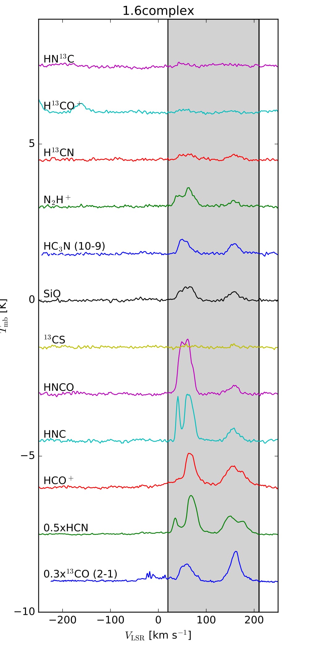
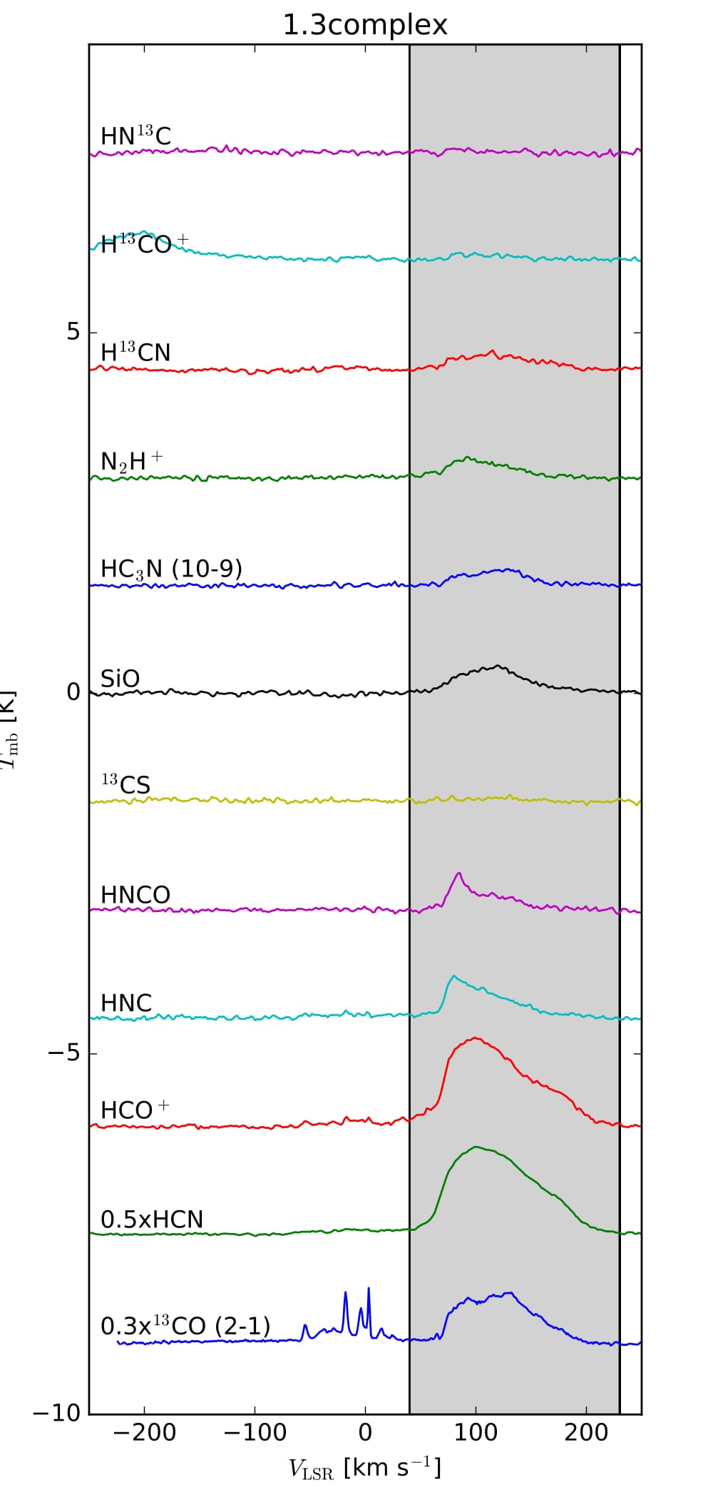
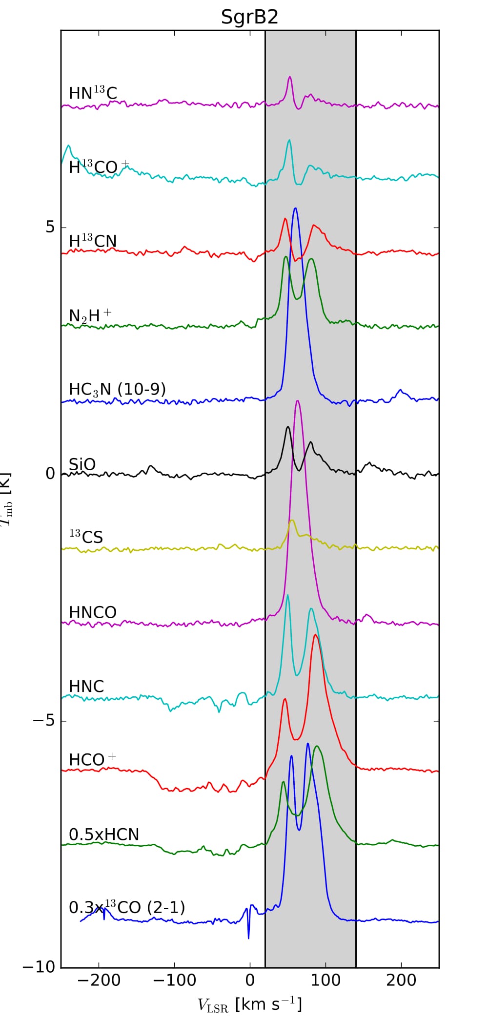
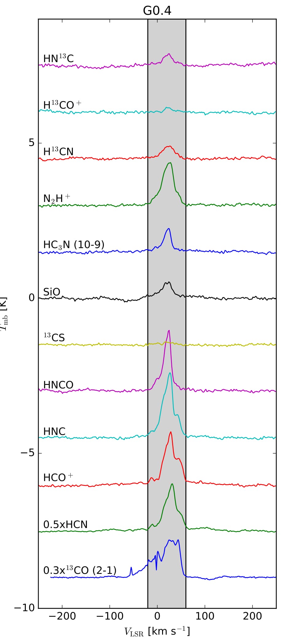
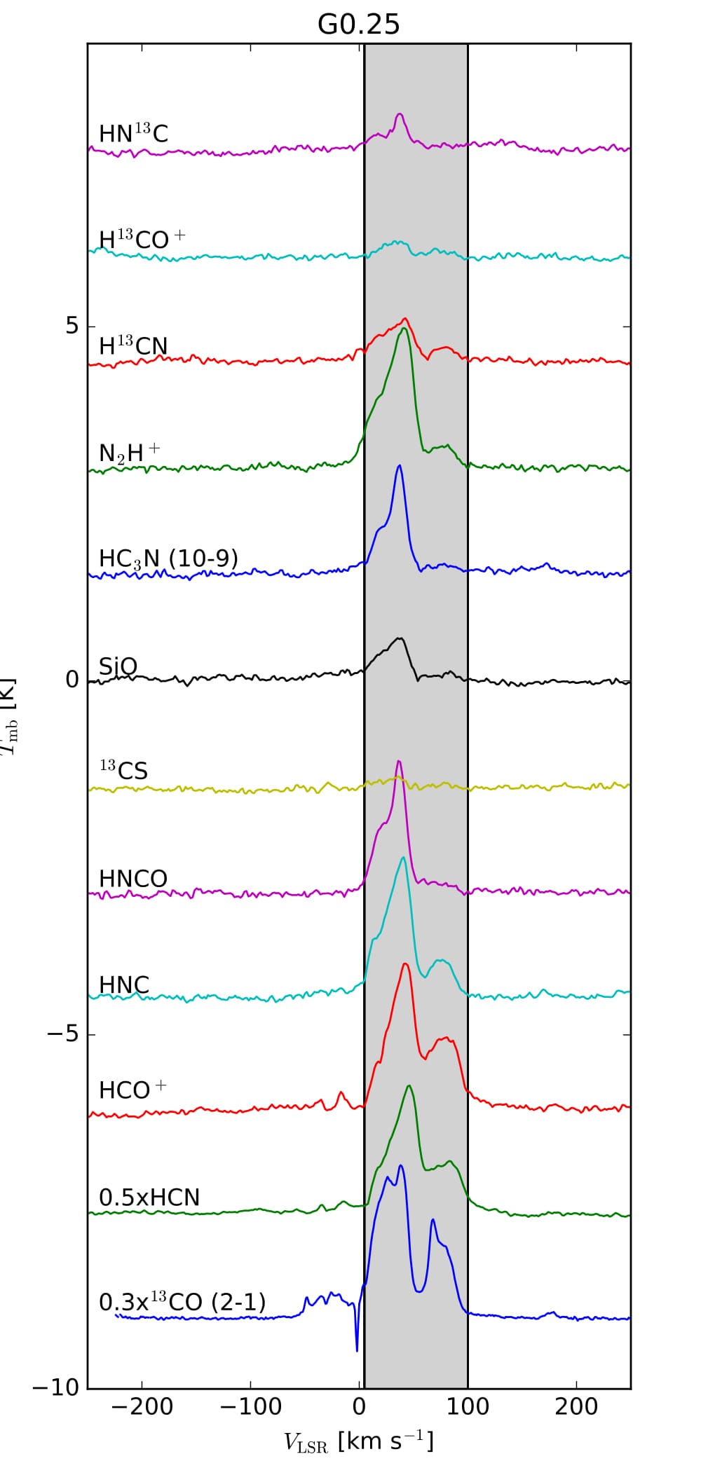
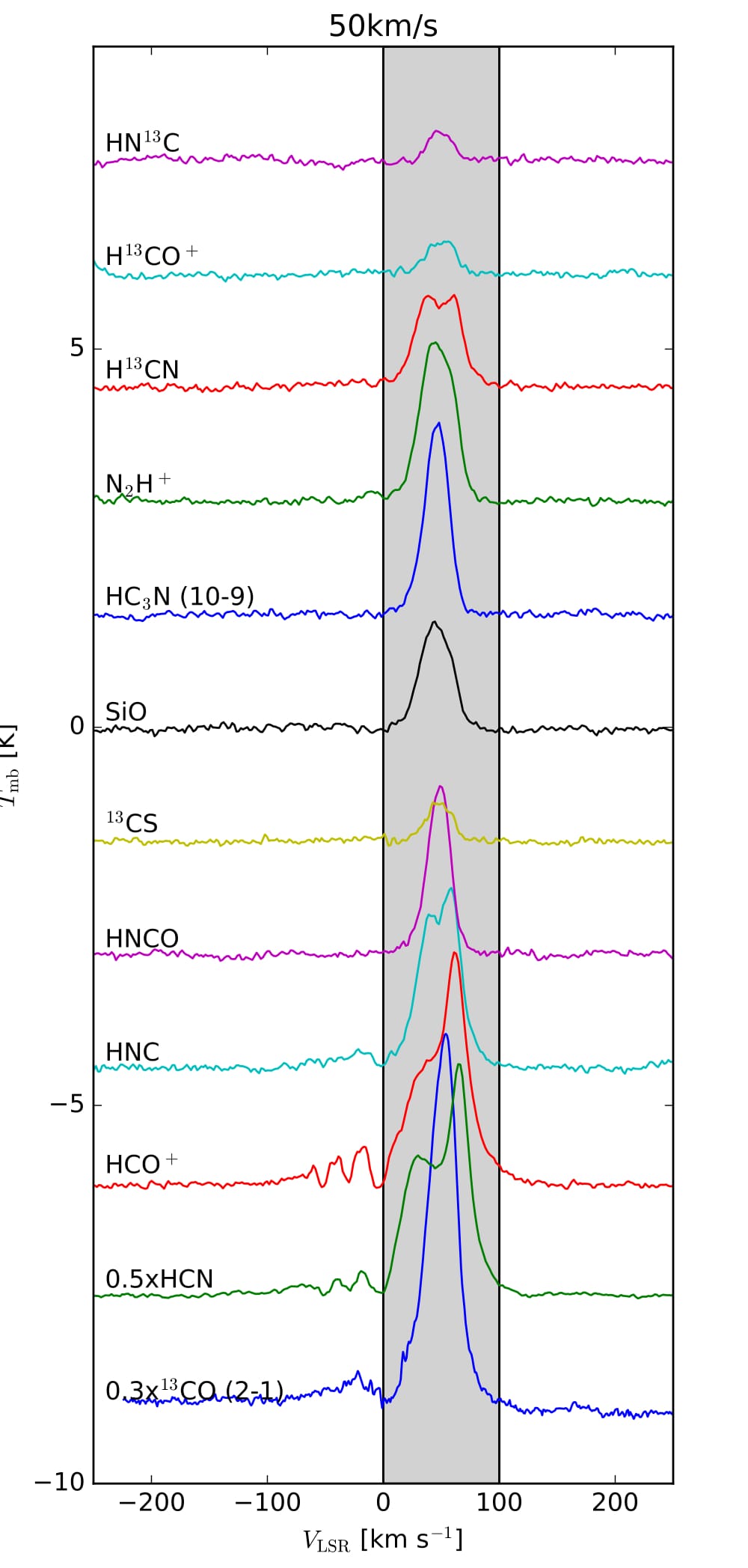
Figure 17: Average spectra for each region shown in Fig. 16. ¹³CO (2-1) spectra are scaled by a factor 0.3 and HCN spectra are scaled by a factor 0.5.

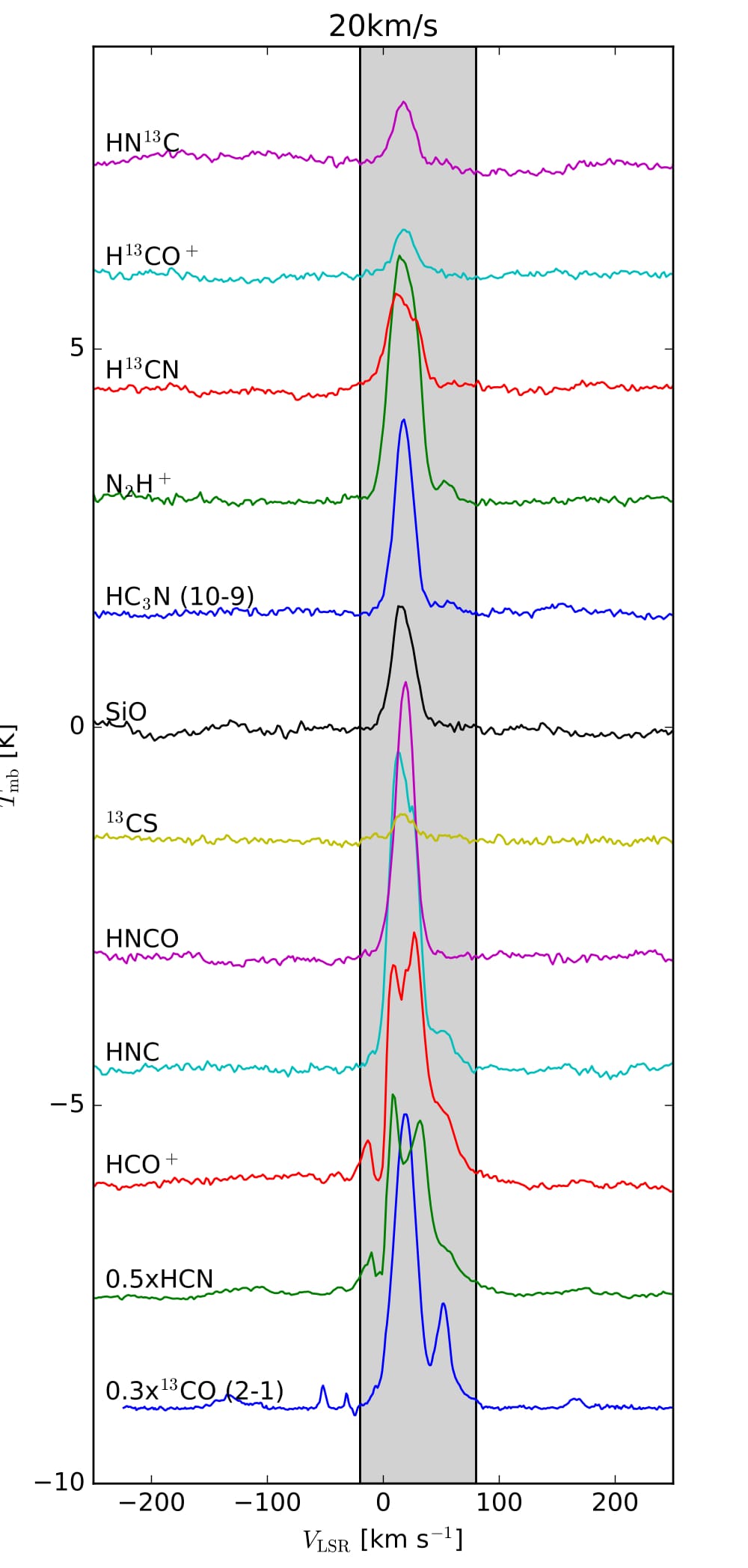
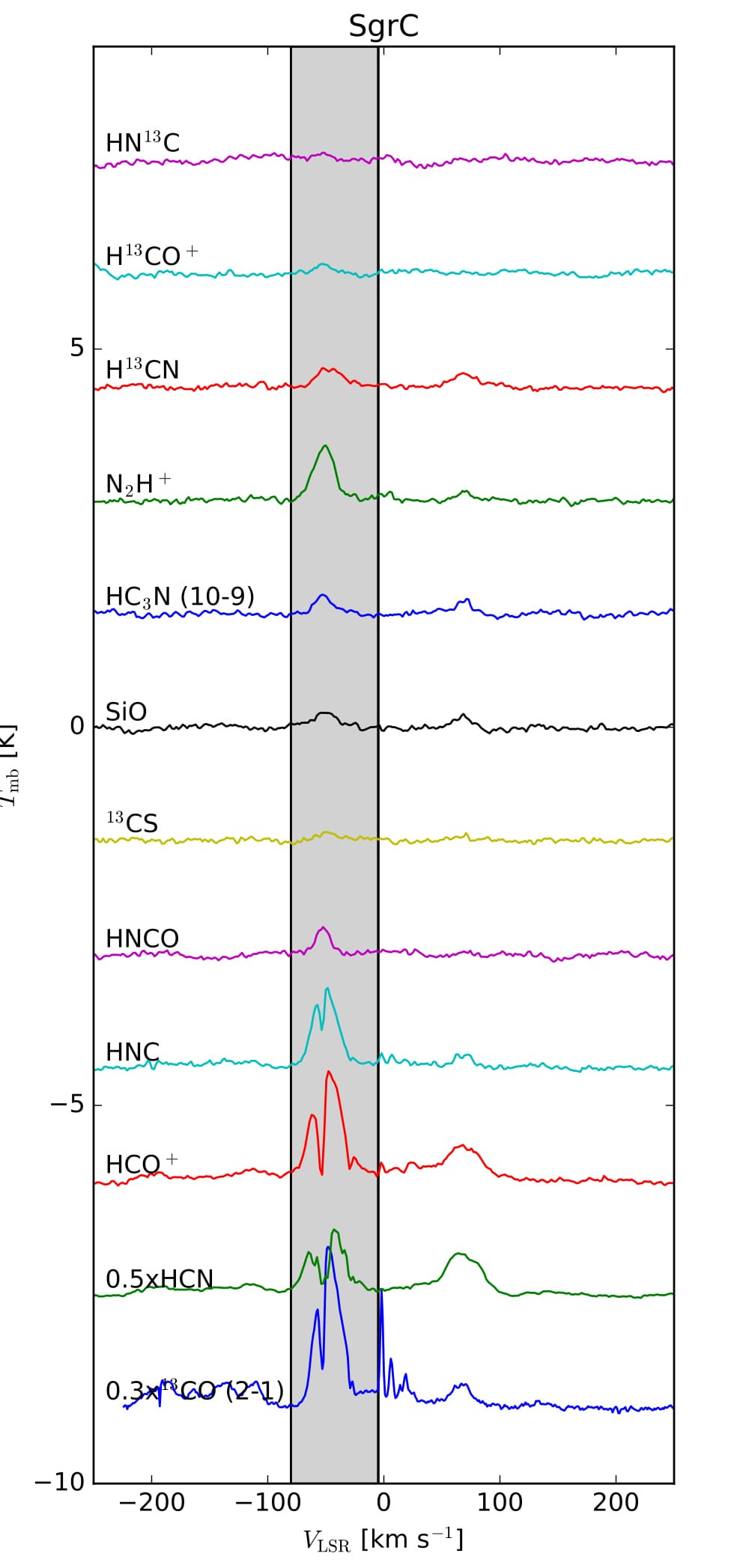
Figure 18: Average spectra for each region shown in Fig. 16. ¹³CO (2-1) spectra are scaled by a factor 0.3 and HCN spectra are scaled by a factor 0.5.

Appendix B Beam efficiency for APEX observations

Since the Galactic center molecular emission is extended in comparison with the beam size, we estimate the beam efficiency for the APEX telescope considering an extended source. Considering the main beam efficiencies measured in November 2012 using Jupiter (see Table 7), we performed a least squares fit for the Ruze formula to get the values for B₀ and $\sigma$ (B${}_{0}=0.69$, $\sigma=0.019$).

$$B_{\rm{eff}}(\lambda)=B_{0}*\exp(-(4\times\pi\times\sigma/\lambda)^{2})$$ (2)

Table 7: Beam efficiencies for APEX telescope using Jupiter

Frequency	Source	Source	Main beam	Forward	Beam
		size	size	efficiency	efficiency
$[$GHz$]$		[”]	[”]
349	Jupiter	44.8	17.6	0.95	0.67
466	Jupiter		13.2	0.95	0.58
691.9	Jupiter	47.4	8.9	0.95	0.49
807.1	Jupiter		7.7	0.95	0.48

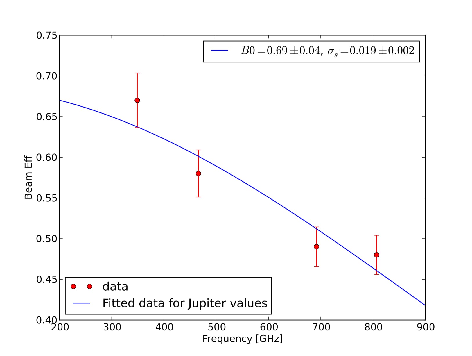
Figure 19: Least squares fit for the values of the main beam efficiency measured on November 2012 at the APEX telescope. We fit the Ruze formula to get the values for B₀ and $\sigma$.

Appendix C Velocity integrated emission

Figure 20: Velocity integrated emission in H¹³CN. From left to right: velocity range from -140 to 20  km s^-1(the complete velocity range covered by the GMLs); velocity range from -140 to -70  km s^-1; -70 to -40  km s^-1, -40 to -20 km s^-1and -20 to 20  km s^-1

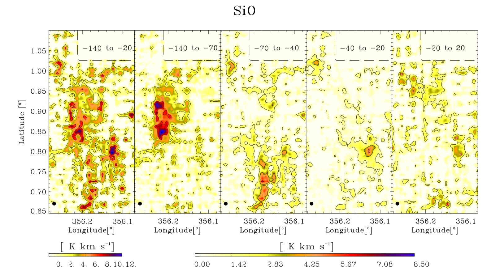
Figure 21: Velocity integrated emission in SiO. From left to right: velocity range from -140 to 20  km s^-1(the complete velocity range covered by the GMLs); velocity range from -140 to -70  km s^-1; -70 to -40  km s^-1, -40 to -20 km s^-1and -20 to 20  km s^-1

Figure 22: Velocity integrated emission in HNCO. From left to right: velocity range from -140 to 20  km s^-1(the complete velocity range covered by the GMLs); velocity range from -140 to -70  km s^-1; -70 to -40  km s^-1, -40 to -20 km s^-1and -20 to 20  km s^-1

Figure 24: Velocity integrated emission in HCO⁺. From left to right: velocity range from -140 to 20  km s^-1(the complete velocity range covered by the GMLs); velocity range from -110 to -70  km s^-1; -70 to -40  km s^-1, -40 to -20 km s^-1and -20 to 20  km s^-1

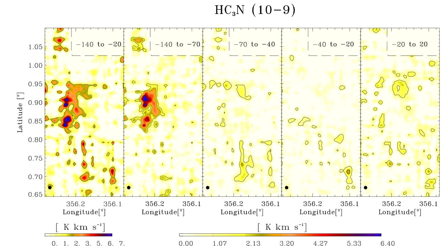
Figure 26: Velocity integrated emission in HC₃N (10-9). From left to right: velocity range from -140 to 20  km s^-1(the complete velocity range covered by the GMLs); velocity range from -140 to -70  km s^-1; -70 to -40  km s^-1, -40 to -20 km s^-1and -20 to 20  km s^-1

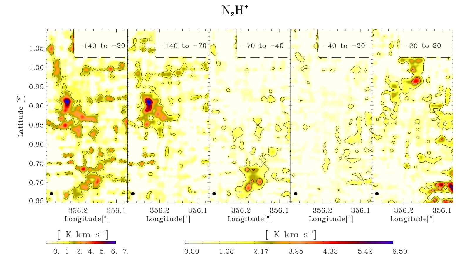
Figure 27: Velocity integrated emission in N₂H⁺. From left to right: velocity range from -140 to 20  km s^-1(the complete velocity range covered by the GMLs); velocity range from -140 to -70  km s^-1; -70 to -40  km s^-1, -40 to -20 km s^-1and -20 to 20  km s^-1

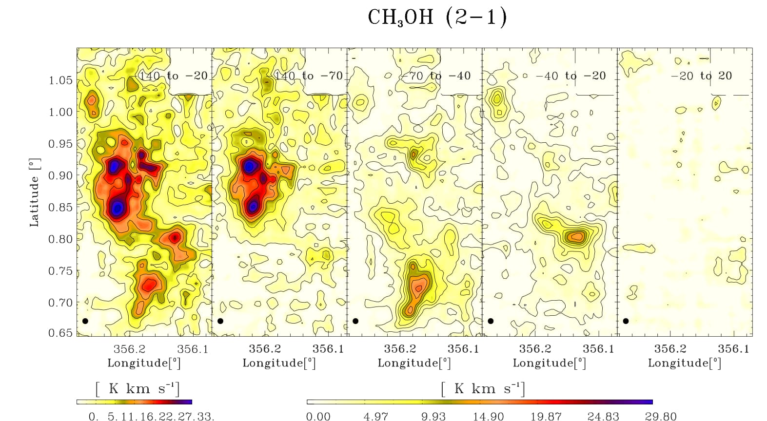
Figure 28: Velocity integrated emission in CH₃OH. From left to right: velocity range from -140 to 20  km s^-1(the complete velocity range covered by the GMLs); velocity range from -140 to -70  km s^-1; -70 to -40  km s^-1, -40 to -20 km s^-1and -20 to 20  km s^-1

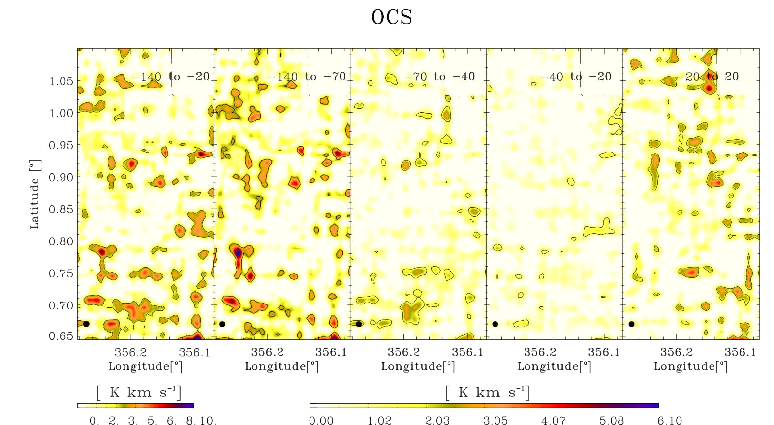
Figure 29: Velocity integrated emission in OCS. From left to right: velocity range from -140 to 20  km s^-1(the complete velocity range covered by the GMLs); velocity range from -140 to -70  km s^-1; -70 to -40  km s^-1, -40 to -20 km s^-1and -20 to 20  km s^-1

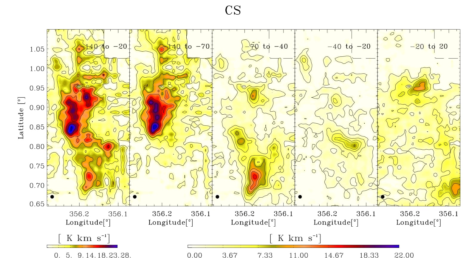
Figure 30: Velocity integrated emission in CS. From left to right: velocity range from -140 to 20  km s^-1(the complete velocity range covered by the GMLs); velocity range from -140 to -70  km s^-1; -70 to -40  km s^-1, -40 to -20 km s^-1and -20 to 20  km s^-1

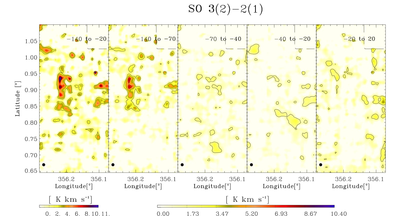
Figure 31: Velocity integrated emission in SO ($3_{2}-2_{1}$). From left to right: velocity range from -140 to 20  km s^-1(the complete velocity range covered by the GMLs); velocity range from -140 to -70  km s^-1; -70 to -40  km s^-1, -40 to -20 km s^-1and -20 to 20  km s^-1

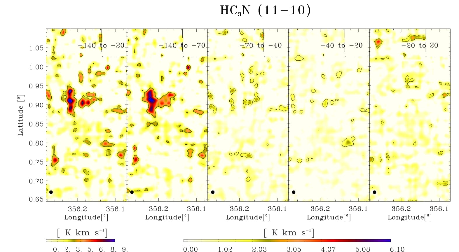
Figure 32: Velocity integrated emission in HC₃N (11-10). From left to right: velocity range from -140 to 20  km s^-1(the complete velocity range covered by the GMLs); velocity range from -140 to -70  km s^-1; -70 to -40  km s^-1, -40 to -20 km s^-1and -20 to 20  km s^-1

Appendix D Latitude-velocity maps

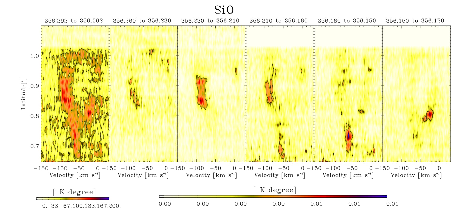
Figure 34: Latitude-velocity maps of the SiO emission integrated in the complete longitude range from 356^∘.29165 to 356^∘.06249 (Left), and in longitude steps of 108” (second panel to the right).

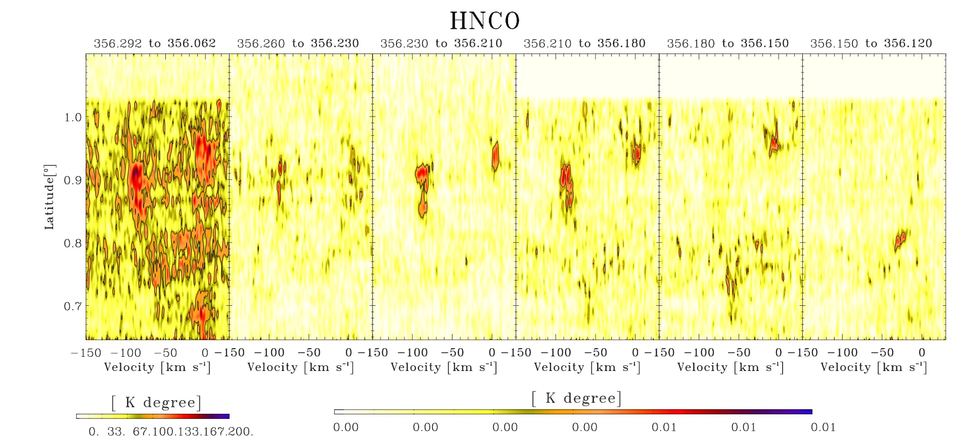
Figure 35: Latitude-velocity maps of the HNCO emission integrated in the complete longitude range from 356^∘.29165 to 356^∘.06249 (Left), and in longitude steps of 108” (second panel to the right).

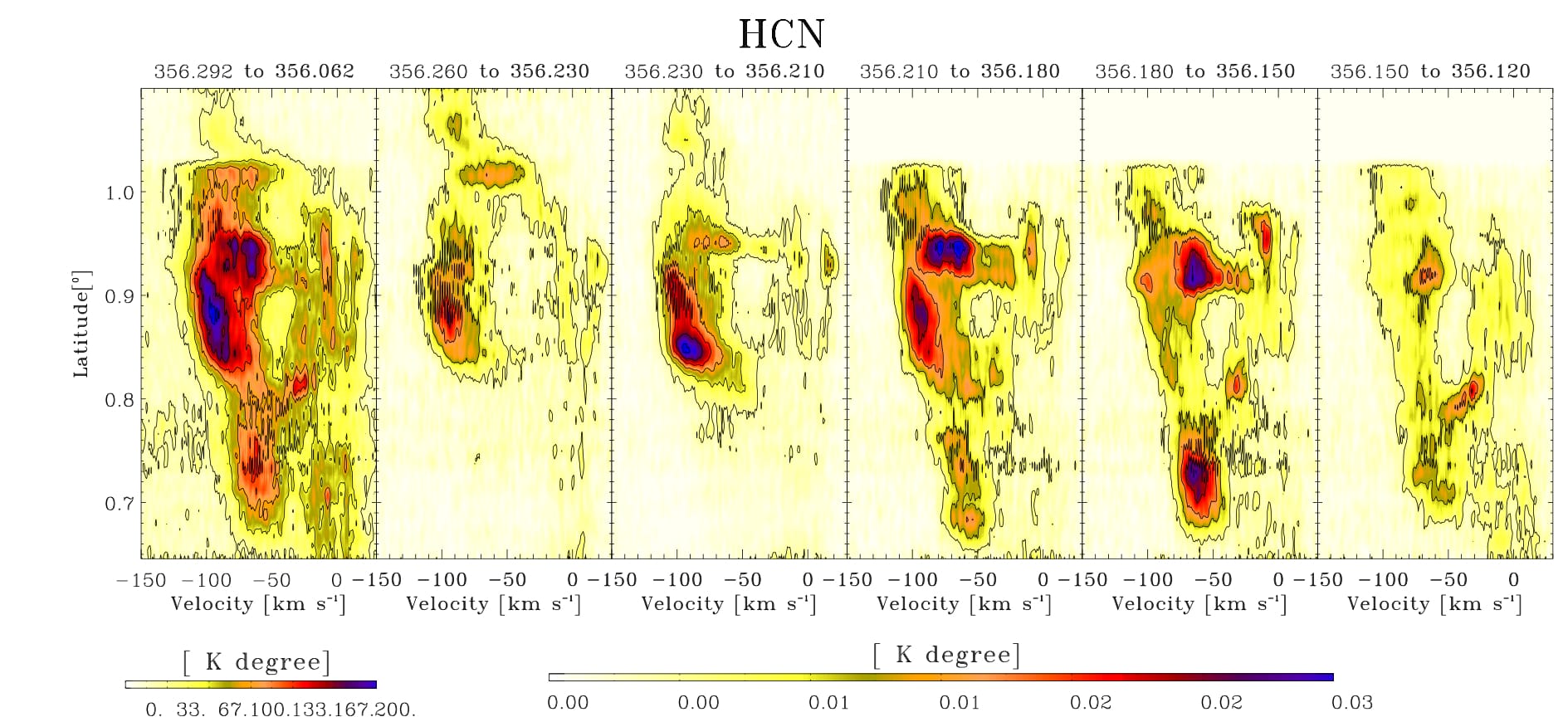
Figure 36: Latitude-velocity maps of the HCN emission integrated in the complete longitude range from 356^∘.29165 to 356^∘.06249 (Left), and in longitude steps of 108” (second panel to the right).

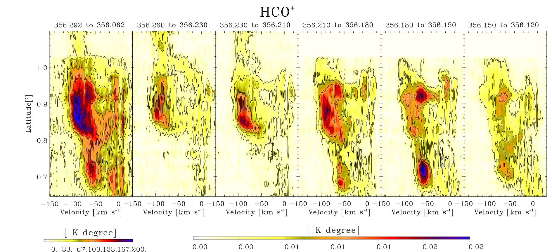
Figure 37: Latitude-velocity maps of the HCO⁺ emission integrated in the complete longitude range from 356^∘.29165 to 356^∘.06249 (Left), and in longitude steps of 108” (second panel to the right).

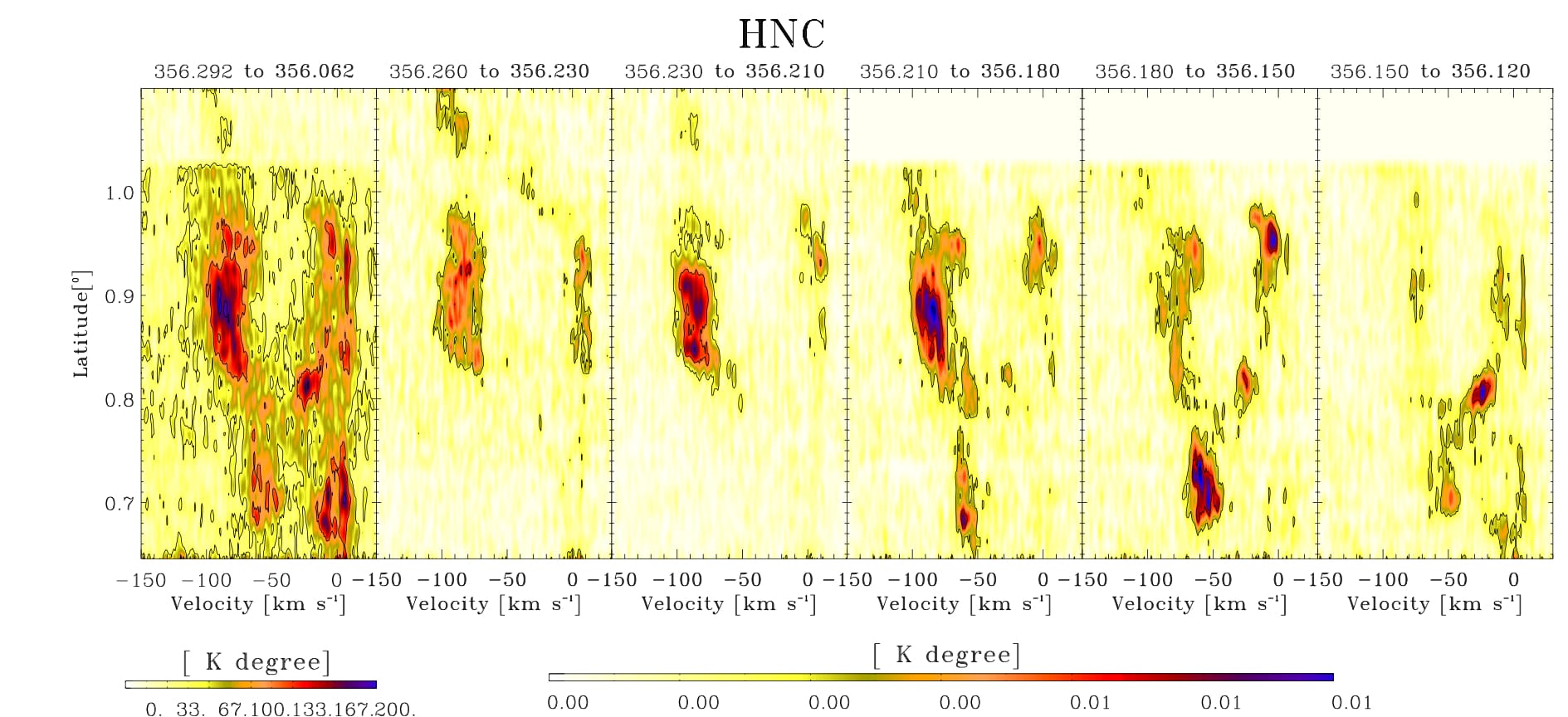
Figure 38: Latitude-velocity maps of the HNC emission integrated in the complete longitude range from 356^∘.29165 to 356^∘.06249 (Left), and in longitude steps of 108” (second panel to the right).

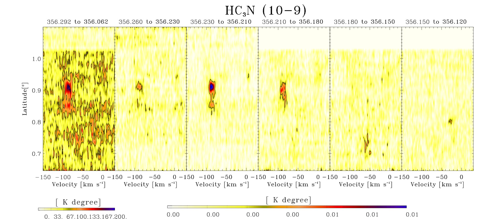
Figure 39: Latitude-velocity maps of the HC₃N (10-9) emission integrated in the complete longitude range from 356^∘.29165 to 356^∘.06249 (Left), and in longitude steps of 108” (second panel to the right).

Figure 40: Latitude-velocity maps of the N₂H⁺ emission integrated in the complete longitude range from 356^∘.29165 to 356^∘.06249 (Left), and in longitude steps of 108” (second panel to the right).

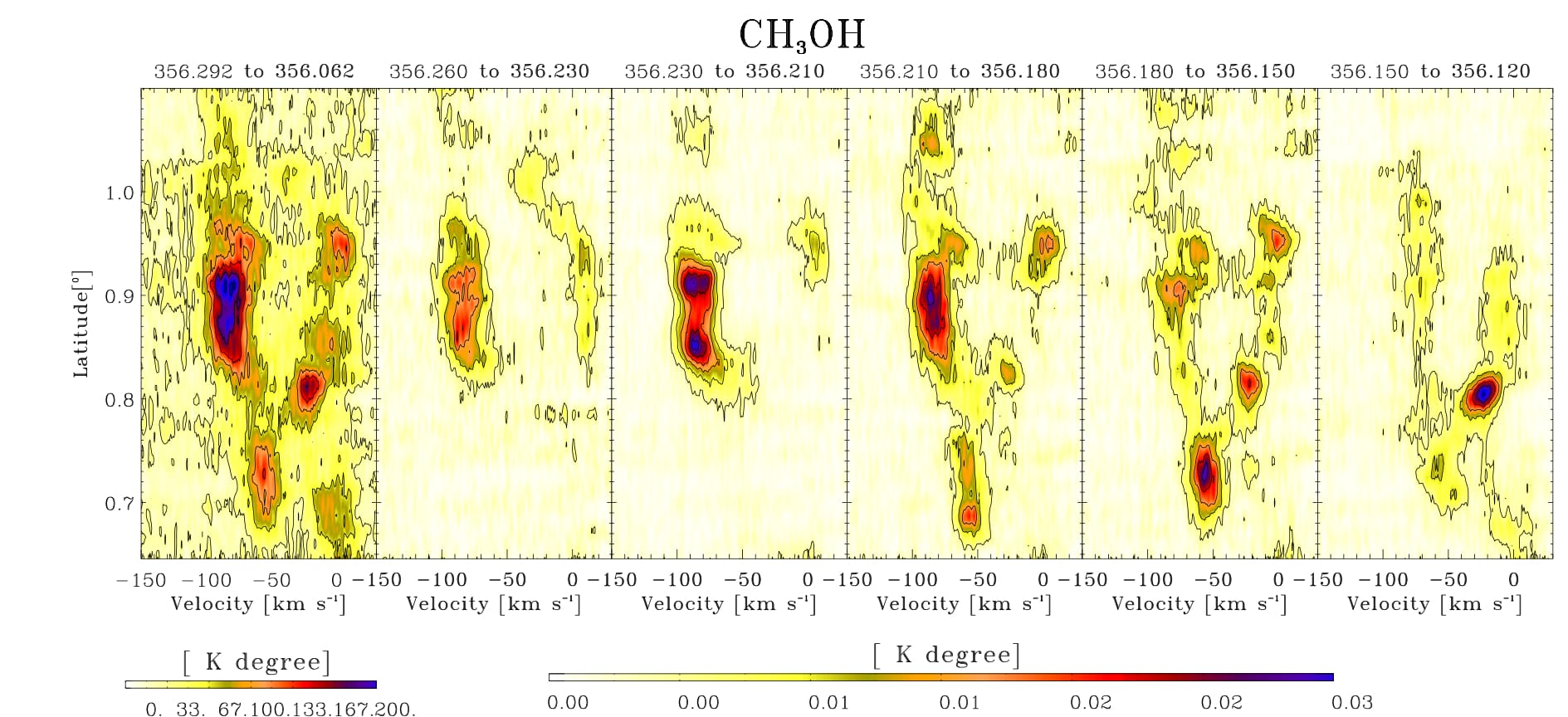
Figure 41: Latitude-velocity maps of the CH₃OH emission integrated in the complete longitude range from 356^∘.29165 to 356^∘.06249 (Left), and in longitude steps of 108” (second panel to the right).

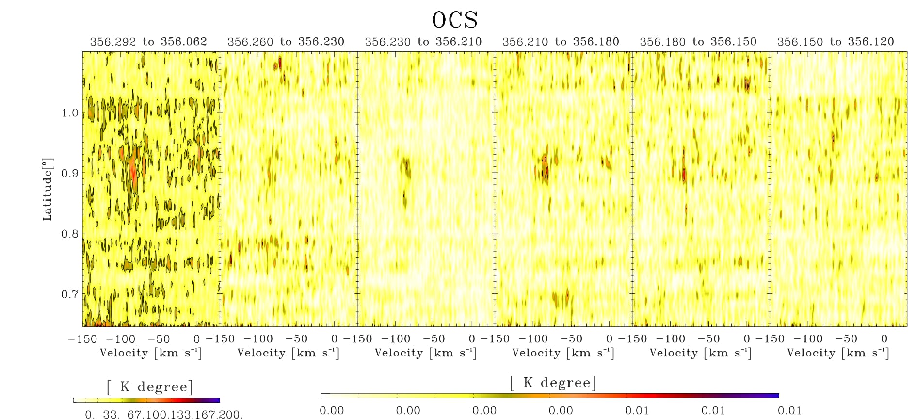
Figure 42: Latitude-velocity maps of the OCS emission integrated in the complete longitude range from 356^∘.29165 to 356^∘.06249 (Left), and in longitude steps of 108” (second panel to the right).

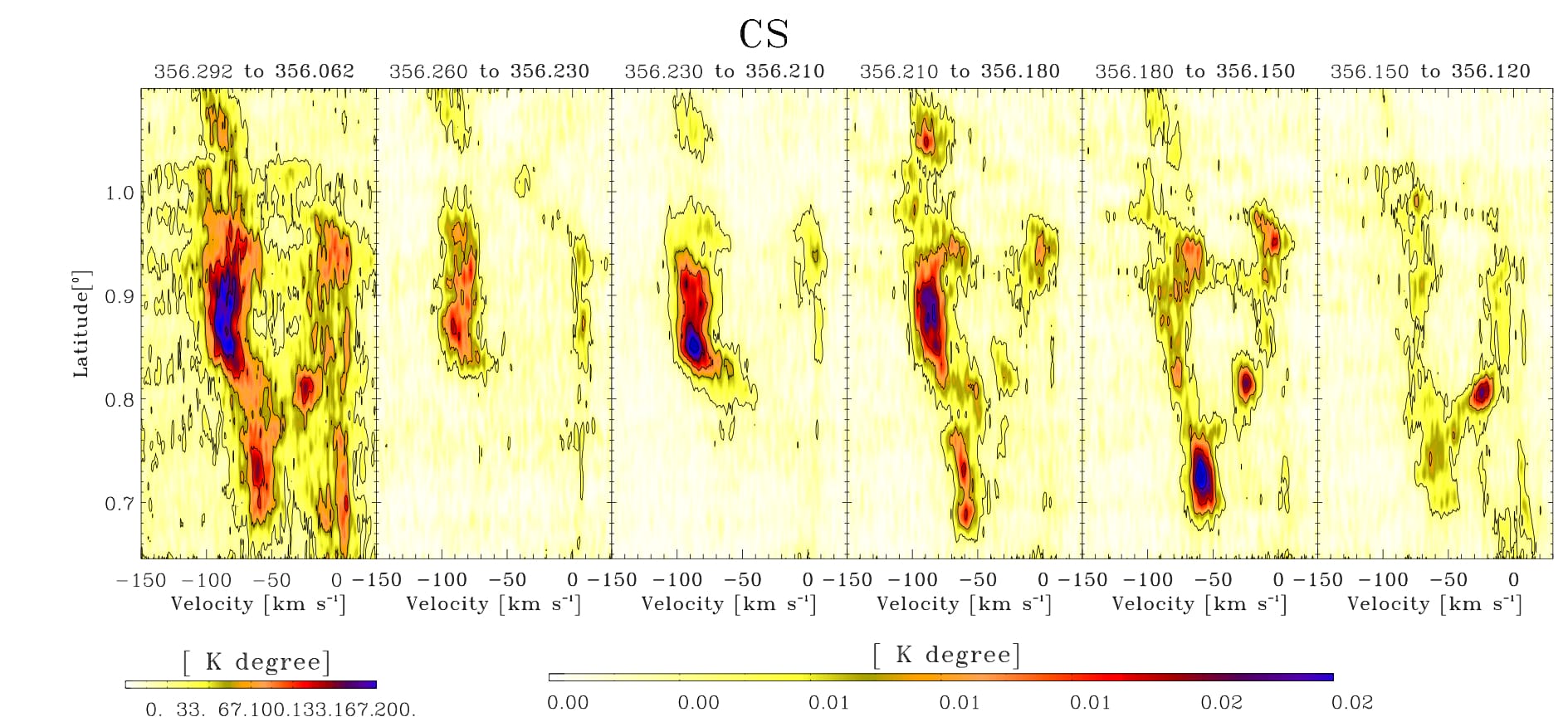
Figure 43: Latitude-velocity maps of the CS emission integrated in the complete longitude range from 356^∘.29165 to 356^∘.06249 (Left), and in longitude steps of 108” (second panel to the right).

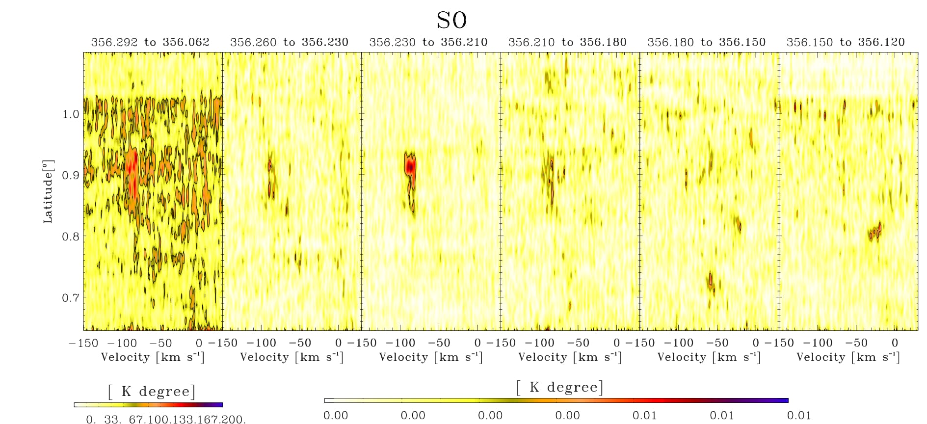
Figure 44: Latitude-velocity maps of the SO emission integrated in the complete longitude range from 356^∘.29165 to 356^∘.06249 (Left), and in longitude steps of 108” (second panel to the right).