Masses of the components of SB2 binaries observed with Gaia. IV. Accurate SB2 orbits for 14 binaries, and masses of 3 binaries

Abstract

The orbital motion of non-contact double-lined spectroscopic binaries (SB2), with periods of a few tens of days to several years, holds unique accurate informations on individual stellar masses, that only long-term monitoring can unlock. The combination of radial velocity measurements from high-resolution spectrographs and astrometric measurements from high-precision interferometers allows the derivation of SB2 components masses down to the percent precision. Since 2010, we observed a large sample of SB2 with the SOPHIE spectrograph at the Observatoire de Haute-Provence, aiming at the derivation of orbital elements with sufficient accuracy to obtain masses of components with relative errors as low as 1% when the astrometric measurements of the Gaia satellite will be taken into account. In this paper we present the results from six years of observations of 14 SB2 systems with periods ranging from 33 to 4185 days. Using the todmor algorithm we computed radial velocities from the spectra, and then derived the orbital elements of these binary systems. The minimum masses of the 28 stellar components are then obtained with a sample average accuracy of 1.0$\pm$0.2 %. Combining the radial velocities with existing interferometric measurements, we derived the masses of the primary and secondary components of HIP 61100, HIP 95995 and HIP 101382 with relative errors for components (A,B) of respectively (2.0, 1.7) %, (3.7, 3.7) %, and (0.2, 0.1) %. Using the Cesam2k stellar evolution code, we could constrain the initial He-abundance, age and metallicity for HIP 61100 and HIP 95995.

1 Introduction

Following the work of papers I-III (Halbwachs et al., 2014, 2016; Kiefer et al., 2016) we propose to measure masses of stars with an accuracy better than 1%. The loosely constrained single stars stellar evolution models still necessitate a confrontation to extremely accurate masses of stars. Non-contact binaries have the exclusive advantage to provide mass measurements of two separate objects with different masses but with the same age. They could thus provide a strong constraint on stellar models (Torres et al., 2012). To that end, we proposed in paper I (Halbwachs et al., 2014) to combine the high-resolution spectroscopy of the Spectrographe pour l’Observation des PHénomènes des Intérieurs Stellaires et des Exoplanètes (SOPHIE; Observatoire de Hautes-Provence) to the high-precision astrometry of the Gaia satellite on high-contrast large-period and bright spectroscopic binaries. SOPHIE provides radial velocities with an accuracy of a few tens of m s^-1, and Gaia will soon deliver photocenter positions with an accuracy of a few tens of microarcseconds. The combination of both will allow achieving better than 1% accuracy on binary masses.

In paper I (Halbwachs et al., 2014), we selected a sample of 68 SB2s for which we expect to reach that level of precision. We have been observing these stars since 2010 with SOPHIE. A first result of our program was the detection of the secondary component in the spectra of 20 binaries which were previously known as single-lined (paper I). A second result was the determination of masses for two particular SB2s with accuracy between 0.26 and 2.4 %, coupling astrometric measurements from PIONIER and radial velocities from SOPHIE (paper II; Halbwachs et al. 2015). In a third paper (paper III; Kiefer et al. 2016), we derived projected masses (M $\sin^{3}i$) with precision better than 1.2% for the two components of 10 binaries, and the masses of the binary HIP 87895 with an accuracy of $\sim$1% thanks to additional astrometric data.

Here, we present the accurate orbits measured for 14 SB2s (Table LABEL:tab:obs) with periods ranging from 33 to 4185 days. After 8 years of observations with SOPHIE, we collected a total of 203 spectra of these stars. A large number of previously published measurements is also available for each of these binaries in the SB9 catalog (Pourbaix et al., 2004). Four of these targets were identified as new SB2s in paper I. We combined the radial velocity (RV) measurements and existing interferometric data for HIP 61100, HIP 95995 and HIP 101382, to derive the masses of their components. This will enable us to validate the masses derived from our RVs and from Gaia astrometry, when the Gaia astrometric transits will be available. Meanwhile, in the present paper, these masses are confronted to evolutionary models.

The observations are presented in Section 2. The method of measurements of radial velocities from SOPHIE’s observations is explained in Section 3. We derive the orbital solutions in Section 4. The derivation of the masses of HIP 61100, HIP 95995 and HIP 101382 is presented in Section 5. Finally, in Section 6 we examine how they compare to stellar evolution models.

2 Observations

The observations were performed at the T193 telescope of the Haute-Provence Observatory, with the SOPHIE spectrograph (Perruchot et al., 2008). SOPHIE is dedicated to the search of extrasolar planets, and, its high resolution ($R$$\sim$$75,000$) enables accurate stellar radial velocities to be measured for SB2 components. Since the beginning of the programme, we have accumulated 49 nights of observations in visitor mode. Before each observation run, ephemerides were derived from existing orbits provided by the SB9 catalogue (Pourbaix et al., 2004), and priority classes were assigned on the basis of the orbital phase and of the observations already performed. In addition, we obtained observations in service mode for a total duration of 7 nights; these observations were essentially used to complete the phase coverage of short-period binaries.

The spectra were all reduced through SOPHIE’s pipeline, including localization of the orders on the frame, optimal order extraction, cosmic-ray rejection, wavelength calibration, flat-fielding and bias subtraction.

Among all the observed SB2s, we have selected those which were satisfying two conditions:

• They were observed over, at least, the part of the phase where the RVs of the components may be derived. Except for HIP 77122, a binary with a period of more than 11 years, the observations covered more than one period.

• They received a minimum of 11 observations. This limit was set for statistical reasons (see e.g. paper III): Although an SB2 orbit could be derived in principle from only 6 of those observations, a minimum of 5 degrees-of-freedom on each component are needed for a reliable rescaling of the RV errorbars to the stochastic noise level, as explained in Section 4.

Table LABEL:tab:obs summarizes this information.

Table 1: The SB2s analyzed in this paper.

Name	Alt. name	V	Perioda	$N_{\text{spec}}$ b	Spanc	SNRd
HIP/HD	HD/BD	(mag.)	(day)		(period)
Previously published SB2
HIP 9121	BD +41 379	9.01	695	16	3.1	48
HIP 21946	HD 285970	9.86	56	11	34	54
HIP 38018	HD 61994	7.08	552	12	3.9	96
HIP 61100	HD 109011	8.10	1284	13	2.8	98
HIP 77122	HD 141335	8.95	4290	12	0.54	48
HIP 95995	HD 184467	6.59	494	14	4.3	145
HIP 100046	HD 193468	6.73	289	18	7.5	136
HIP 101382	HD 195987	7.09	57	18	45	101
HIP 116360	HD 221757	7.22	348	15	9.8	97
HD 98031	BD +13 2380	8.40	271	15	7.9	48
SB2s identified in paper I, previously published as SB1s
HIP 7143	HD 9312	6.81	37	16	59	143
HIP 12472	HD 16646	8.10	329	13	6.7	90
HIP 48895	HD 86358	6.46	34	17	87	140
HIP 72706	HD 131208	7.61	84	13	18	97

3 Radial velocity measurements

The radial velocities of the components are derived using the TwO-Dimensional cross-CORrelation algorithm todcor (Zucker & Mazeh, 1994; Zucker et al., 2004). It calculates the cross-correlation of an SB2 spectrum and two best-matching stellar atmosphere models, one for each component of the observed binary system. The radial velocities of both components are measured at the optimum of this two-dimensional cross-correlation function (CCF). More specifically we employed the multi-order version of todcor that is named todmor (Zucker et al., 2004). We redirect the readers to our preceding articles (paper I-III) for more details on this algorithm.

All SOPHIE multi-orders spectra were first corrected for the blaze using the response function provided by SOPHIE’s pipeline; then for each of them, the pseudo-continuum was detrended using a p-percentile filter (paper II, Hodgson et al., 1985). Finally, before deriving the RVs, a best-matching model spectrum is determined for both SB2 components of each star.

3.1 Optimizing the model spectra

The theoretical spectra from the PHOENIX stellar atmosphere models (Husser et al., 2013) optimized for best-matching of the components of all 14 SB2s are given in Table 2. Contrary to the method presented in previous papers, instead of optimizing the CCF for all orders, we minimized the $\chi^{2}$ of the selected spectra compared to the PHOENIX models around the Ca I line at $\sim$6120 Å(order 33). This line is particularly sensitive to $T_{\text{eff}}$ and $\log g$ if conditions are close to LTE (Drake, 1991; Mashonkina et al., 2007). Moreover being on the red side of the spectrum it offers the best conditions with respect to signal-to-noise and strength of the second component. We used the full order $\#$ 33, which also incorporates a few Fe lines. Compared to the previous method explained in paper III, which consisted in optimizing the CCF, the above method led to more reliable values of stellar parameters, with in particular less biased values of metallicity. We verified that the two methods give consistent, and equally satisfying, results on radial velocities measurements.

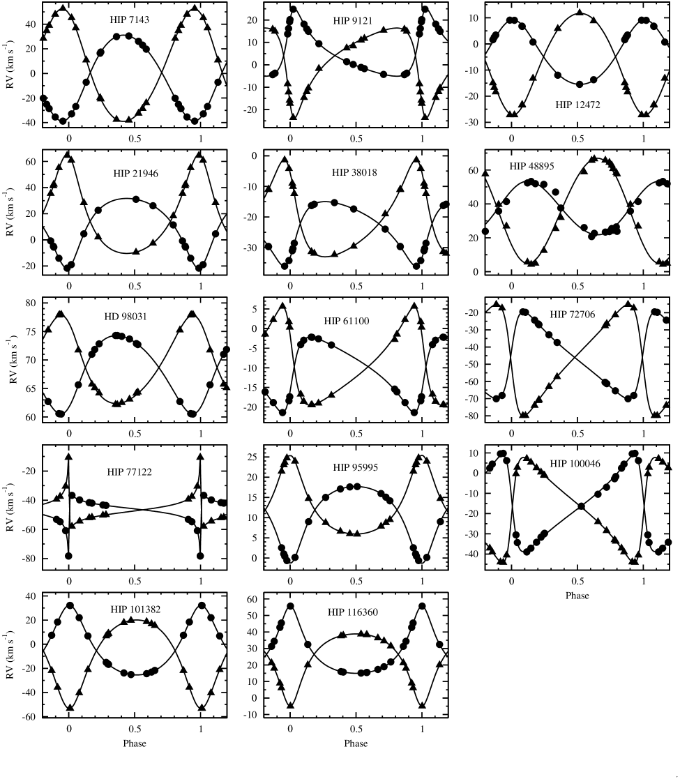
Figure 1: The spectroscopic orbits of the 14 SB2; the circles refer to the SOPHIE RVs of the primary component, and the triangles to the secondary. For each SB2, the RVs are shifted to the zero point of the SOPHIE measurements of the primary component.

We optimized the values of effective temperature $T_{\text{eff}}$, rotational broadening $v\sin i$, metallicity [Fe/H], surface gravity $\log(g)$, and flux ratio at $4916$ Å, $\alpha$$=$$F_{2}/F_{1}$. For binaries on the main sequence, if $\alpha$ is too low ($\alpha$$<$$0.1$) and the secondary $\log g$ cannot be properly derived, we fixed its value with respect to $T_{\text{eff}}$, following the empirical relation $\log g=12-2\log T_{\text{eff}}$, as derived from Fig. 1 of Angelov (1996). Each theoretical spectrum is convolved with the instrument line spread function, here modeled by a Gaussian, and pseudo-continuum detrended with the same techniques employed for detrending the observed spectra.

The values of the stellar parameters, and their uncertainties, given in Table 2 are the average and standard deviation of the individual estimations. The 1$\sigma$ uncertainties do not include known systematics, see e.g. Torres et al. (2012). To give a point of comparison, we measured the Sun’s parameters on SOPHIE spectra of Vesta and Ceres in Table 2. Metallicity was found to be off by $-0.12$ dex, $\Delta T_{\text{eff},\odot}$$\sim$$60$ K, and $\Delta\log(g)_{\odot}$$\sim$$0.1$. Given their small amplitude, and lacking an exhaustive analysis of benchmark stars spectra with this method, these errors could be considered as more realistic minimum uncertainties on $T_{\text{eff}}$, $\log(g)$ and [Fe/H], than the values given in Table 2. Furthermore, the uncertainty on the effective temperatures is actually larger than this, since varying by hand metallicity in a $\pm$0.1 dex range for a few targets, we found an amplitude of variations of $T_{\text{eff}}$ on the order of 100-200 K.

Table 2: The stellar parameters of the 14 SB2, determined by $\chi^{2}$ optimization around the Ca I line at 6121 Å. Sun’s parameters derived with the same protocol are given in the last row.

HIP	a ​$T_{\text{eff,1}}$	b ​$\log g_{1}$	c ​$V_{1}\sin i_{1}$	d ​$[\text{Fe/H}]$	$\alpha$
HD	$T_{\text{eff,2}}$	$\log g_{2}$	$V_{2}\sin i_{2}$
	(K)	(dex)	(km s-1)	(dex)	(flux ratio)
HIP 7143	5367	4.30	4.7	0.03	0.063
	$\pm$166	$\pm$0.13	$\pm$0.6	$\pm$0.03	$\pm$0.013
	5150	4.6${}_{\text{\tiny MS}}$	$<$8
	$\pm$228
HIP 9121	5789	4.40	2.7	0.11	0.083
	$\pm$21	$\pm$0.03	$\pm$0.3	$\pm$0.01	$\pm$0.010
	4544	4.89	$<$2
	$\pm$164	$\pm$0.10
HIP 12472	6253	4.4${}_{\text{\tiny MS}}$	10.5	-0.86	0.037
	$\pm$82		$\pm$0.3	$\pm$0.12	$\pm$0.012
	4802	4.6${}_{\text{\tiny MS}}$	$<$4
	$\pm$292
HIP 21946	4680	4.72	4.0	-0.13	0.035
	$\pm$21	$\pm$0.05	$\pm$0.4	$\pm$0.03	$\pm$0.004
	4164	4.8${}_{\text{\tiny MS}}$	$<$10
	$\pm$110
HIP 38018	5585	4.46	3.5	-0.04	0.069
	$\pm$13	$\pm$0.04	$\pm$0.2	$\pm$0.06	$\pm$0.011
	4484	4.7${}_{\text{\tiny MS}}$	$<$5
	$\pm$110
HIP 48895	6186	4.30	74.1	-0.59	0.253
	$\pm$152	$\pm$0.09	$\pm$2.5	$\pm$0.08	$\pm$0.010
	5697	4.69	21.4
	$\pm$79	$\pm$0.10	$\pm$1.0
HIP 61100	5105	4.75	5.7	-0.14	0.229
	$\pm$21	$\pm$0.10	$\pm$0.1	$\pm$0.10	$\pm$0.004
	4175	4.8	5.1
	$\pm$35	$\pm$0.1	$\pm$0.4
HIP 72706	4524	3.27	4.3	-0.13	0.099
	$\pm$8	$\pm$0.03	$\pm$0.4	$\pm$0.01	$\pm$0.023
	5272	4.50	2.9
	$\pm$280	$\pm$0.11	$\pm$1.1
HIP 77122	5638	4.22	$<$4	-1	0.195
	$\pm$45	$\pm$0.24			$\pm$0.060
	5035	4.60	$<$3
	$\pm$131	$\pm$0.31
HIP 95995	5114	4.62	2.7	-0.33	0.524
	$\pm$11	$\pm$0.05	$\pm$0.3	$\pm$0.01	$\pm$0.083
	4705	4.67	2.7
	$\pm$101	$\pm$0.05	$\pm$1.0
HD 98031	6018	4.55	2.4	-0.13	0.236
	$\pm$8	$\pm$0.07	$\pm$0.7	$\pm$0.04	$\pm$0.001
	5095	4.86	$<$3
	$\pm$19	$\pm$0.07
HIP 100046	6069	4.28	26.2	-0.71	0.585
	$\pm$53	$\pm$0.21	$\pm$1.0	$\pm$0.06	$\pm$0.016
	5623	4.36	13.7
	$\pm$43	$\pm$0.21	$\pm$0.5
HIP 101382	5296	4.71	3.9	-0.38	0.156
	$\pm$19	$\pm$0.03	$\pm$0.3	$\pm$0.01	$\pm$0.005
	4360	4.97	$<$2
	$\pm$87	$\pm$0.04
HIP 116360	6227	4.37	4.3	-0.21	0.624
	$\pm$68	$\pm$0.09	$\pm$0.4	$\pm$0.02	$\pm$0.026
	5915	4.49	3.5
	$\pm$10	$\pm$0.09	$\pm$1.1
Sun	5836	4.58	4.9	-0.12
	$\pm$40	$\pm$0.10	$\pm$0.2	$\pm$0.04

3.2 Deriving radial velocities

We then applied todmor to all multi-order spectra of each target and determined the radial velocities of both components discarding all orders harboring strong telluric lines, following the method of paper III.

In the cases where the S/N ratio and the secondary-to-primary flux ratio were large enough (SNR$>$90 and $\alpha$$>$$0.1$), we incorporated an enhancement on the 2D-CCF calculation. We employed the first-derivative of the spectra, rather than the spectra themselves. Using first derivative is equivalent to applying a linear filter on the spectra, filtering out low frequency components (like e.g. the continuum). Unfortunately, it enhances high frequency noise, and for that reason cannot be used on low S/N ratio spectra. We found that it greatly reduces systematics on RV measurements of those binaries with strong blend.

Final velocities for each component are displayed in Table 3. They are used to derive the orbital solutions for the 14 SB2s in the next section.

Table 3: New radial velocities from SOPHIE and obtained with todmor. The uncertainties must still be corrected as explained in Section 4. Outliers are marked with an asterisk (^∗) and are not taken into account in the analysis.

HIP 7143
BJD	$RV_{1}$	$\sigma_{RV1}$	$RV_{2}$	$\sigma_{RV2}$	$O_{1}-C_{1}$	$O_{2}-C_{2}$
-2400000	km s-1	km s-1	km s-1	km s-1	km s-1	km s-1
2455440.5949	-28.6137	0.0087	39.5047	0.0869	-0.0112	-0.2463
2455532.3039	29.9337	0.0088	-36.9342	0.0868	-0.0103	0.0246
2455783.6041	17.3891	0.0087	-20.3808	0.0806	-0.0093	0.1403
2455864.4055	30.4795	0.0089	-37.6110	0.0869	0.0215	0.0213
2456148.5899	16.4093	0.0087	-19.2077	0.0891	-0.0247	0.0498
2456243.3400	-25.1332	0.0087	35.2395	0.0865	0.0346	-0.0113
2456323.2855	-32.9010	0.0091	45.6786	0.0881	-0.0284	0.3327
2456525.5388∗	-6.8752∗	0.0087∗	-26.1124∗	0.1173∗	-29.9263∗	1.8151∗
2456525.5489	23.0257	0.0087	-28.0582	0.0882	0.0047	-0.1701
2456526.5759	19.7230	0.0087	-23.4145	0.0856	0.0054	0.1453
2456619.4717	-7.1678	0.0088	11.3499	0.0840	-0.0101	-0.3033
2456889.5967	26.0816	0.0089	-31.9416	0.0877	0.0086	-0.0546
2457009.3357	-20.1976	0.0088	28.8898	0.0874	0.0199	0.1252
2457414.3022	-35.4380	0.0109	48.4965	0.1051	0.0110	-0.2250
2457602.5998	-26.8715	0.0087	37.4743	0.0842	-0.0264	0.0259
2457635.5346	-38.7686	0.0087	53.2214	0.0843	0.0135	0.1327

HIP 9121
BJD	$RV_{1}$	$\sigma_{RV1}$	$RV_{2}$	$\sigma_{RV2}$	$O_{1}-C_{1}$	$O_{2}-C_{2}$
-2400000	km s-1	km s-1	km s-1	km s-1	km s-1	km s-1
2455440.6065	-4.4125	0.0097	15.9387	0.0857	-0.0110	0.3651
2455532.3126	20.1786	0.0097	-17.2062	0.0868	-0.0138	0.0057
2455605.3068	18.1418	0.0109	-14.5813	0.0939	-0.0412	-0.0481
2455864.4267	0.1595	0.0102	8.4879	0.0950	-0.0357	-0.9579
2456147.5908	-3.7162	0.0089	15.0394	0.0794	0.0164	0.3576
2456243.3503	24.8212	0.0098	-23.5053	0.0845	0.0156	-0.1438
2456323.3008	14.9387	0.0099	-10.3337	0.0958	0.0112	-0.1404
2456525.6005	1.4133	0.0100	7.5680	0.0781	-0.0094	-0.2414
2456618.4926	-1.6987	0.0099	11.8527	0.0976	0.0128	-0.1348
2456913.4916	16.2085	0.0099	-12.0895	0.0840	0.0032	-0.1928
2456919.4382	19.2128	0.0106	-15.7803	0.0949	-0.0096	0.1384
2457009.3471	16.0572	0.0093	-11.9517	0.0823	0.0135	-0.2704
2457073.2958	9.4184	0.0103	-1.5753	0.1178	0.0239	1.2421
2457295.6294	-1.1549	0.0095	11.0601	0.0913	0.0282	-0.2231
2457414.3261	-4.2774	0.0176	15.4326	0.1592	-0.0186	0.0493
2457603.5503	13.7650	0.0098	-8.4294	0.0887	-0.0101	0.2277

HIP 12472
BJD	$RV_{1}$	$\sigma_{RV1}$	$RV_{2}$	$\sigma_{RV2}$	$O_{1}-C_{1}$	$O_{2}-C_{2}$
-2400000	km s-1	km s-1	km s-1	km s-1	km s-1	km s-1
2455532.4082	1.6055	0.0441	-14.5375	0.0810	-0.0746	0.4260
2455605.3484	6.6888	0.0809	-22.8412	0.1327	0.0108	0.0023
2455783.6130	-13.7153	0.0469	9.2047	0.0741	-0.0131	-0.0843
2455864.5337	2.5696	0.0443	-16.3092	0.0803	0.0459	-0.0156
2455933.2717	6.7945	0.0901	-23.0360	0.1543	-0.0399	0.0543
2456148.6166∗	-8.1223∗	0.0412∗	2.5239∗	0.0800∗	0.1609∗	1.7787∗
2456243.3940	9.0360	0.0451	-26.7895	0.0804	0.0032	-0.2332
2456525.5750	3.4028	0.0455	-18.0037	0.0779	0.0256	-0.3644
2456618.5243	0.6876	0.0438	-12.7734	0.0642	0.0213	0.5918
2456889.6184	9.0899	0.0443	-26.7878	0.0744	0.0123	-0.1609
2457009.3760	-11.9803	0.0427	6.2414	0.0842	-0.0057	-0.3238
2457603.5777	0.9406	0.0407	-12.9910	0.0671	-0.0580	0.8981
2457721.5573	-15.4946	0.0431	12.2045	0.0737	-0.0072	0.1008

HIP 21946
BJD	$RV_{1}$	$\sigma_{RV1}$	$RV_{2}$	$\sigma_{RV2}$	$O_{1}-C_{1}$	$O_{2}-C_{2}$
-2400000	km s-1	km s-1	km s-1	km s-1	km s-1	km s-1
2455864.5931	30.9873	0.0119	-9.4994	0.1903	0.0049	-0.0450
2456243.5337	22.6048	0.0129	2.1410	0.2291	0.0031	-0.2630
2456323.4334	26.0735	0.0130	-2.6027	0.1837	-0.0138	-0.0747
2456619.5802	-5.5830	0.0129	42.5907	0.2249	-0.0007	0.3067
2457009.4399	11.3879	0.0126	18.2601	0.1442	-0.0030	-0.0070
2457014.5018	-4.8917	0.0128	41.3349	0.2290	-0.0147	0.0489
2457020.4023	-21.7157	0.0124	64.5834	0.2309	0.0133	-0.5478
2457073.3398	-14.1075	0.0134	55.1816	0.2816	-0.0206	0.8638
2457295.6463	-0.8778	0.0125	35.4673	0.2188	0.0024	-0.1632
2457699.5165	-18.9958	0.0149	60.8245	0.2310	-0.0132	-0.4207
2457761.3441	4.5465	0.0131	28.4629	0.2285	0.0065	0.5018

HIP 38018
BJD	$RV_{1}$	$\sigma_{RV1}$	$RV_{2}$	$\sigma_{RV2}$	$O_{1}-C_{1}$	$O_{2}-C_{2}$
-2400000	km s-1	km s-1	km s-1	km s-1	km s-1	km s-1
2455605.4554	-15.8212	0.0080	-31.6573	0.0610	-0.0658	-0.0322
2455966.3859	-29.6282	0.0076	-10.8293	0.0617	0.0218	-0.0811
2456034.3241	-36.0742	0.0115	-1.1332	0.1010	-0.0046	-0.0305
2456243.6090	-15.3134	0.0076	-32.0804	0.0613	0.0189	0.1804
2456324.3742	-17.3822	0.0075	-29.3241	0.0780	0.0105	-0.1591
2456619.6080	-31.0369	0.0075	-8.7959	0.0653	0.0025	-0.1352
2456700.4676	-16.2770	0.0084	-31.0950	0.0668	0.0377	-0.3103
2457009.5244	-23.9774	0.0072	-18.7759	0.0526	-0.0100	0.5106
2457073.3764	-29.7104	0.0062	-10.6737	0.0518	0.0035	-0.0214
2457159.3587	-34.2367	0.0087	-3.9517	0.0743	-0.0118	-0.0772
2457728.6301	-30.3165	0.0072	-9.8280	0.0596	-0.0067	-0.0711
2457734.6292	-28.5850	0.0070	-12.1420	0.0588	-0.0027	0.2105

HIP 48895
BJD	$RV_{1}$	$\sigma_{RV1}$	$RV_{2}$	$\sigma_{RV2}$	$O_{1}-C_{1}$	$O_{2}-C_{2}$
-2400000	km s-1	km s-1	km s-1	km s-1	km s-1	km s-1
2455966.4971	41.4163	0.1379	27.6481	0.0794	-2.7001	3.7556
2456243.6398	51.9407	0.1321	5.7655	0.0789	-0.3817	-2.0201
2456323.5312	26.0378	0.1738	59.6220	0.0749	1.6606	-3.0149
2456414.3350	51.5298	0.1408	13.2361	0.0804	2.6904	-1.3861
2456619.6215	46.9870	0.2076	26.1839	0.0769	5.5179	-2.9049
2456701.4324	25.4852	0.1369	63.5982	0.0748	0.4116	2.3281
2456764.3623	22.6437	0.1384	67.3399	0.0753	0.6953	-0.0644
2457009.5859	35.7275	0.1334	40.4026	0.0801	-2.0947	4.1557
2457073.4027	26.4163	0.1506	59.2057	0.0701	-0.9983	2.5305
2457160.3757	37.5641	0.1408	32.6651	0.0771	-0.2168	-3.6628
2457505.3652	20.7102	0.1568	66.4075	0.0792	-1.5991	-0.2883
2457759.6114	53.2215	0.1481	5.0854	0.0833	0.0073	-0.9498
2457792.3706	52.3538	0.1550	6.4234	0.0860	-1.0702	0.8000
2454845.6013	23.3993	0.1296	66.5367	0.0702	0.6445	0.7153
2454846.6471	23.7001	0.1339	65.2222	0.0700	-0.3565	1.9559
2454847.6167	24.5010	0.1368	61.5615	0.0692	-1.2396	1.6006
2454848.6314	23.7993	0.1569	58.3759	0.0726	-4.1640	2.7777

Table 3: Continued.

HIP 98031
BJD	$RV_{1}$	$\sigma_{RV1}$	$RV_{2}$	$\sigma_{RV2}$	$O_{1}-C_{1}$	$O_{2}-C_{2}$
-2400000	km s-1	km s-1	km s-1	km s-1	km s-1	km s-1
2455692.3492	72.8755	0.0109	64.6313	0.0348	0.0058	0.2213
2455933.6379	74.1453	0.0179	62.9888	0.0565	-0.0012	0.0166
2455966.5107	72.7083	0.0107	64.8335	0.0326	0.0266	0.2119
2456324.4501	62.7036	0.0129	75.7316	0.0386	0.0783	-0.2146
2456414.3490	70.9941	0.0109	66.2017	0.0307	-0.0852	-0.2245
2456619.6559	60.5365	0.0104	78.3963	0.0308	0.0011	0.0967
2456700.5552	72.8220	0.0106	64.6617	0.0330	-0.0164	0.2165
2456763.4017	73.6712	0.0104	63.6086	0.0334	0.0479	0.0473
2457009.6140	74.2814	0.0104	62.6262	0.0324	0.0175	-0.2138
2457159.3958	60.6343	0.0136	78.2756	0.0403	0.0247	0.0597
2457160.3675	60.5873	0.0109	78.3338	0.0325	0.0103	0.0811
2457436.6010	60.5133	0.0104	78.4542	0.0308	-0.0138	0.1452
2457471.5766	65.6334	0.0133	72.2121	0.0384	-0.0192	-0.3250
2457505.3820	71.8385	0.0108	65.6050	0.0305	-0.0450	0.0844
2457819.5101	74.2800	0.0102	62.6705	0.0316	0.0109	-0.1636

HIP 61100
BJD	$RV_{1}$	$\sigma_{RV1}$	$RV_{2}$	$\sigma_{RV2}$	$O_{1}-C_{1}$	$O_{2}-C_{2}$
-2400000	km s-1	km s-1	km s-1	km s-1	km s-1	km s-1
2454124.7212	-2.1884	0.0123	-19.3714	0.0703	0.0204	0.0195
2454889.6065∗	-14.1818∗	0.0147∗	-4.7802∗	0.0840∗	-0.0628∗	-0.9102∗
2455306.4091	-4.0880	0.0110	-16.6121	0.0709	0.0729	0.2349
2455605.5531	-4.1704	0.0095	-16.9148	0.0623	-0.0524	-0.0118
2456243.6803	-16.1346	0.0096	-1.3190	0.0642	-0.0225	-0.0463
2456323.5971	-18.8578	0.0095	2.4018	0.0570	-0.0414	0.1503
2456413.3839	-21.4210	0.0121	5.7921	0.0727	-0.0032	0.1504
2456619.6953	-2.9770	0.0095	-18.4678	0.0569	0.0052	-0.0846
2456700.5934	-2.2159	0.0096	-19.3730	0.0534	0.0059	0.0011
2456763.5299	-2.6145	0.0109	-18.9232	0.0639	0.0107	-0.0748
2457505.4205	-15.4310	0.0093	-2.6677	0.0635	0.0064	-0.5160
2457759.6959	-18.4149	0.0092	1.8460	0.0559	-0.0069	0.1266
2457767.6521	-17.3820	0.0088	0.4519	0.0530	0.0041	0.0643

HIP 72706
BJD	$RV_{1}$	$\sigma_{RV1}$	$RV_{2}$	$\sigma_{RV2}$	$O_{1}-C_{1}$	$O_{2}-C_{2}$
-2400000	km s-1	km s-1	km s-1	km s-1	km s-1	km s-1
2456033.5020	-61.2850	0.0075	-25.7871	0.1070	-0.0192	0.1112
2456147.3536	-19.4972	0.0073	-79.3190	0.1022	0.0474	0.1668
2456324.5831	-26.9623	0.0074	-70.0314	0.0976	-0.0366	-0.0260
2456414.4587	-32.8521	0.0073	-62.4272	0.1031	-0.0029	-0.0302
2456700.6800	-60.4920	0.0073	-27.0406	0.1136	-0.0494	-0.0850
2457073.6330	-24.3145	0.0067	-73.3307	0.0989	-0.0167	0.0499
2457159.4832	-26.5475	0.0072	-70.5603	0.0951	-0.0049	-0.0631
2457470.6254	-68.1682	0.0082	-16.7236	0.1115	0.0102	0.2961
2457475.6035∗	-49.3856∗	0.0154∗	-43.8833∗	0.1826∗	0.0671∗	-2.8120∗
2457505.5470	-37.3135	0.0072	-56.6873	0.1064	-0.0023	-0.0213
2457542.3640	-65.4462	0.0146	-21.0450	0.2545	-0.0316	-0.4755
2457542.4266	-65.4616	0.0077	-20.7041	0.1106	0.0008	-0.1960
2457550.5131	-70.0817	0.0076	-14.6032	0.1050	0.0109	-0.0421
2457819.5824	-19.7787	0.0072	-79.2520	0.1005	-0.0295	-0.0292

HIP 77122
BJD	$RV_{1}$	$\sigma_{RV1}$	$RV_{2}$	$\sigma_{RV2}$	$O_{1}-C_{1}$	$O_{2}-C_{2}$
-2400000	km s-1	km s-1	km s-1	km s-1	km s-1	km s-1
2455306.5079∗	-49.1723∗	0.0097∗	-44.2639∗	0.0300∗	-0.4494∗	-0.5203∗
2456033.5194	-53.1250	0.0125	-38.9871	0.0349	0.0055	-0.2407
2456148.3858	-54.7882	0.0124	-37.0043	0.0349	0.0060	-0.1444
2456324.6472	-60.8632	0.0117	-30.0466	0.0327	-0.0091	-0.0572
2456413.5714	-78.1954	0.0120	-10.2543	0.0345	0.0058	0.0674
2456414.4769	-78.2975	0.0119	-10.1390	0.0331	-0.0017	0.0754
2456525.3381	-36.6294	0.0119	-57.4821	0.0337	0.0001	-0.0273
2456764.5216	-39.7897	0.0115	-53.8866	0.0328	-0.0018	-0.0126
2457073.6595	-41.6506	0.0108	-51.5984	0.0312	0.0179	0.1433
2457159.4975	-42.0369	0.0112	-51.2538	0.0320	0.0088	0.0604
2457505.5611	-43.2999	0.0115	-49.8530	0.0337	-0.0202	0.0621
2457602.3944	-43.5835	0.0118	-49.5196	0.0359	-0.0104	0.0628

HIP 95995
BJD	$RV_{1}$	$\sigma_{RV1}$	$RV_{2}$	$\sigma_{RV2}$	$O_{1}-C_{1}$	$O_{2}-C_{2}$
-2400000	km s-1	km s-1	km s-1	km s-1	km s-1	km s-1
2455440.3925	14.1543	0.0130	9.6101	0.0166	-0.0109	-0.0654
2455693.5801	14.9946	0.0122	8.8627	0.0158	-0.0041	0.0420
2455784.4255	17.5962	0.0115	6.1163	0.0152	-0.0029	-0.0379
2456034.6088	0.4528	0.0115	23.7456	0.0151	-0.0055	0.0139
2456243.2705	17.0740	0.0116	6.7064	0.0153	0.0032	0.0105
2456414.5806	15.0522	0.0122	8.8434	0.0159	0.0010	0.0765
2456525.3813	1.0363	0.0114	23.1434	0.0150	0.0034	0.0009
2456618.3725	8.9973	0.0123	14.8330	0.0160	0.0057	-0.1480
2456890.4648	15.9419	0.0118	7.9785	0.0157	0.0063	0.1185
2457295.3224	17.6864	0.0114	6.0110	0.0151	0.0012	-0.0548
2457295.3224	17.6864	0.0114	6.0110	0.0151	0.0012	-0.0548
2457505.6066	2.5417	0.0113	21.5832	0.0148	-0.0038	-0.0081
2457525.5532	-0.6032	0.0115	24.8503	0.0149	-0.0002	0.0303
2457556.4625	0.1786	0.0114	24.0395	0.0147	-0.0016	0.0225

HIP 100046
BJD	$RV_{1}$	$\sigma_{RV1}$	$RV_{2}$	$\sigma_{RV2}$	$O_{1}-C_{1}$	$O_{2}-C_{2}$
-2400000	km s-1	km s-1	km s-1	km s-1	km s-1	km s-1
2455440.3983	-2.7679	0.0647	-32.9372	0.0372	-1.1721	-0.1793
2455693.5912	-10.4280	0.0563	-24.0270	0.0345	-0.8709	0.0598
2455864.2976	-30.1345	0.0683	-0.9387	0.0389	0.7532	-0.0845
2456034.6180	2.4505	0.0598	-37.1059	0.0326	-0.0083	0.0681
2456147.4411	-31.6547	0.0562	0.5238	0.0309	0.5029	-0.0051
2456414.5964	-37.1051	0.0567	5.3736	0.0328	-0.4000	-0.1083
2456525.4010	-16.3540	0.0549	-16.7767	0.0341	-0.1247	0.0429
2456619.3099	4.4352	0.0994	-38.9722	0.0569	0.3452	-0.0215
2456890.4961	-1.6800	0.0535	-33.6484	0.0312	-0.7823	-0.1301
2456940.3394	6.2028	0.0551	-40.5074	0.0332	0.5430	0.1531
2457159.5328	-6.9649	0.0548	-28.4290	0.0332	-1.2451	-0.1627
2457295.3591	-34.1782	0.0474	2.6393	0.0291	0.0230	-0.1154
2457505.6238	9.5644	0.0521	-43.9000	0.0317	0.9413	-0.0121
2457511.5904	9.7700	0.0514	-44.1377	0.0300	0.8712	0.0506
2457539.5993	-30.5416	0.0526	-0.3724	0.0314	0.4782	0.3380
2457542.4749	-34.3064	0.0557	2.8589	0.0337	-0.1168	0.1167
2457563.5620	-38.9690	0.0490	7.1852	0.0301	-0.7511	0.0556
2457602.4760	-29.7396	0.0512	-1.1213	0.0315	0.8755	0.0298

Table 3: Continued.

HIP 101382
BJD	$RV_{1}$	$\sigma_{RV1}$	$RV_{2}$	$\sigma_{RV2}$	$O_{1}-C_{1}$	$O_{2}-C_{2}$
-2400000	km s-1	km s-1	km s-1	km s-1	km s-1	km s-1
2455306.6279∗	27.4215∗	0.0056∗	-48.4736∗	0.0279∗	-0.5988∗	-0.7284∗
2455440.4752	-16.0573	0.0065	8.1802	0.0339	-0.0550	-0.0675
2456147.4603	-23.0348	0.0069	17.0744	0.0350	0.0072	-0.1270
2456243.2796	-16.4840	0.0068	9.0005	0.0344	0.0097	0.1278
2456525.4373	-7.2323	0.0064	-2.7826	0.0362	0.0153	0.1050
2456889.4781∗	-24.9314∗	0.0604∗	18.7325∗	0.3251∗	-0.0833∗	-0.7662∗
2456890.5346	-24.3951	0.0065	18.8520	0.0332	-0.0102	-0.0576
2456906.5610	7.4644	0.0066	-21.5996	0.0337	-0.0098	0.0128
2456914.4368	32.1885	0.0062	-53.0538	0.0316	-0.0126	0.0088
2456922.2759	6.8794	0.0065	-20.9364	0.0328	-0.0106	-0.0670
2457159.5648	-15.0283	0.0065	7.0422	0.0331	0.0041	0.0282
2457160.5553	-16.6925	0.0065	9.1756	0.0331	0.0054	0.0433
2457295.3722	-21.7360	0.0058	15.6240	0.0282	0.0032	0.0795
2457568.5135	-23.8142	0.0066	18.2184	0.0341	0.0142	0.0166
2457571.5894	-25.1569	0.0091	19.9035	0.0466	0.0011	0.0106
2457602.4876	32.1200	0.0066	-52.9594	0.0333	-0.0002	0.0005
2457606.3739	22.0613	0.0122	-40.1714	0.0607	0.0035	-0.0100
2457883.6019	18.4379	0.0065	-35.5057	0.0317	0.0264	0.0179

HIP 116360
BJD	$RV_{1}$	$\sigma_{RV1}$	$RV_{2}$	$\sigma_{RV2}$	$O_{1}-C_{1}$	$O_{2}-C_{2}$
-2400000	km s-1	km s-1	km s-1	km s-1	km s-1	km s-1
2454339.5767	15.9868	0.0096	37.7172	0.0119	-0.0488	-0.0609
2454345.4505	15.7252	0.0107	38.0853	0.0130	-0.0111	-0.0142
2454408.3317	15.4871	0.0096	38.3689	0.0118	-0.0028	0.0047
2454852.2873	31.2565	0.0198	21.3992	0.0241	-0.0501	0.0261
2455784.5553	15.0810	0.0119	38.8450	0.0147	0.0180	0.0222
2456147.5212	15.4694	0.0122	38.4331	0.0150	0.0177	0.0278
2456525.4971	17.2681	0.0116	36.4516	0.0140	0.0056	-0.0084
2456618.4151	45.4494	0.0117	6.1845	0.0144	-0.0116	0.0170
2456889.5524	18.9561	0.0111	34.6675	0.0136	-0.0164	0.0445
2456962.3075	42.7728	0.0077	9.0399	0.0095	-0.0214	0.0075
2456990.3484	55.6703	0.0113	-4.7991	0.0138	0.00001	0.0007
2457295.4256	34.3595	0.0097	18.0903	0.0119	-0.0182	0.0164
2457295.4256	34.3595	0.0097	18.0903	0.0119	-0.0182	0.0164
2457603.5447	21.8455	0.0108	31.5873	0.0131	0.0589	-0.0127
2457732.2988	32.4490	0.0109	20.1658	0.0134	0.0062	0.0133

4 The SB2 orbits

The orbits derived from the RVs in Table 3 have too large residuals in relation to uncertainties. This is clear when the $F_{2}$ indicator of the goodness-of-fit (GOF) is calculated (see paper II, equation 1): the values are too large to obey a normal distribution, because the uncertainties were underestimated. This results in underestimating the uncertainties of the parameters of the orbit, but also in assigning erroneous weights to the RVs of each component. Deriving an SB2 orbital solution necessitates attributing realistic errors to each dataset properly. The correction process was already used in paper III, we refer the reader to that paper for explanations. The corrected errors express as follow with respect to initial errorbars $\sigma_{RV}$:

$$\sigma^{\text{corr}}_{RV,1} =\varphi_{1}\times\sqrt{\sigma_{RV,1}^{2}+\varepsilon_{1}^{2}}$$ (1)

$$\sigma^{\text{corr}}_{RV,2} =\varphi_{2}\times\sqrt{\sigma_{RV,2}^{2}+\varepsilon_{2}^{2}}$$ (2)

The correction terms $\varphi_{1}$, $\varphi_{2}$, $\varepsilon_{1}$ and $\varepsilon_{2}$ are given in Table LABEL:tab:corsigRVprev. The references of previously published RVs are also displayed in this table, as well as the related correction terms.

The orbital solutions of the 14 SB2s were derived twice: from the SOPHIE RVs alone, and also combining them with the previously published RVs. The results are presented on Table LABEL:tab:orbSB2.

Only the period, $P$, the time of periastron passage, $T_{0}$, and the SOPHIE offset $d_{n-p}$ were taken from the combined solution, since $P$ and $T_{0}$ are more accurate than in the SOPHIE solution. The eccentricity $e$, the center-of-mass velocity $\gamma$, the periastron longitude $\omega$, the RV amplitudes $K_{1}$ and $K_{2}$ and the deducted minimum masses and minimum semi-major axes were all taken from the SOPHIE solution. The primary offset $d_{2-1}$ also refers to this solution. The secondary component velocities are often shifted by up to a few 100 m s^-1 compared primary’s velocities (paper II-III). This $d_{2-1}$ incorporates such shift as an additional parameter to the RV fit.

Table 4: Correction terms applied to the uncertainties of the previous and of the new RV measurements. The composition of these terms into a uncertainty correction is set out in Section 4, eqs. 1 and 2. When the original publication provides only weights for the previous measurements, $\varphi_{1,p}$ and $\varphi_{2,p}$ are the uncertainties corresponding to $W=1$, for the primary and for the secondary component, respectively.

HIP/HD	Reference of previous RV	Correction terms for previous measurements				Correction terms for new measurements
		$\varepsilon_{1,p}$	$\varphi_{1,p}$	$\varepsilon_{1,p}$	$\varphi_{2,p}$	$\varepsilon_{1,n}$	$\varphi_{1,n}$	$\varepsilon_{2,n}$	$\varphi_{2,n}$
		km s-1		km s-1		km s-1		km s-1
HIP 7143	Katoh et al. (2013)	0.017	1	$\ldots$	$\ldots$	0.0129	0.947	0.1768	0.947
HIP 9121	Goldberg et al. (2002)	0	0.599	0	3.962	0.0232	0.937	0.5146	0.937
HIP 12472	CGG95a	0	0.674	$\ldots$	$\ldots$	0	1.049	0.2515	1.049
HIP 21946	HMU12a	0	1	0	1	0.0068	1.116	0.2676	1.116
HIP 38018	DM88a	0	1	$\ldots^{b}$	$\ldots^{b}$	0.0338	0.921	0.2519	0.921
HIP 48895	Griffin (2006)c	$\ldots$	$\ldots$	0	1.409	1.4918	1.054	0.6993	1.054
HD 98031	Griffin (2005b)	0	0.316	0	0.822	0.0233	0.961	0.2224	0.961
HIP 61100	Halbwachs et al. (2003)	0	0.7359	1.467	1	0.0196	1.021	0.1965	1.021
HIP 72706	Massarotti et al. (2008)	0	1	$\ldots$	$\ldots$	0.0267	1.208	0	1.208
HIP 77122	Goldberg et al. (2002)d	0.770	1	3.416	1	0.0085	1.083	0.0993	1.083
HIP 95995	Pourbaix (2000)	0	1.070	0	1.060	0	0.489	0.0736	0.953
HIP 100046	Griffin (2005c)e	0	0.471	0	0.404	0.7031	1.060	0.0905	1.060
HIP 101382	Torres et al. (2002)	0	0.316	0	1.422	0.0206	0.938	0.0658	0.938
HIP 116360	Griffin (2005a)	0	0.325	0	0.433	0.0272	0.982	0.0238	0.982

Table 5: The orbital elements of the 14 SB2s. Apart for HIP 77122, $P$ and $T_{0}$ were derived from the previously published RV measurements and from the new ones, but the other elements correspond to the new RVs alone. The radial velocity of the barycentre, $V_{0}$, is in the reference system of the new measurements of the primary component. The minimum masses and minimum semi-major axes are derived from the true period ($P_{true}=P\times(1-V_{0}/c)$). The numbers in parentheses refer to the previously published RV measurements

HIP	$P$	$T_{0}$(BJD)	$e$	$V_{0}$	$\omega_{1}$	$K_{1}$	${\cal M}_{1}\sin^{3}i$	$a_{1}\sin i$	$N_{1}$	$d_{n-p}$	$\sigma(O_{1}-C_{1})$
HD/BD						$K_{2}$	${\cal M}_{2}\sin^{3}i$	$a_{2}\sin i$	$N_{2}$	$d_{2-1}$	$\sigma(O_{2}-C_{2})$
	(d)	2400000+		(km s-1)	(o)	(km s-1)	(${\cal M}_{\odot}$)	(Gm)		(km s-1)	(km s-1)
HIP 7143	36.519182	56614.6542	0.14321	0.7726	203.418	34.9715	1.0971	17.3808	15	-2.7542	0.012
HD 9312	$\pm 0.000031$	$\pm 0.0057$	$\pm 0.00018$	$\pm 0.0040$	$\pm 0.073$	$\pm 0.0057$	$\pm 0.0033$	$\pm 0.0028$	(12)	$\pm 0.0085$	(0.019)
						45.821	0.8373	22.773	15	0.490	0.173
						$\pm 0.065$	$\pm 0.0014$	$\pm 0.032$		$\pm 0.049$
HIP 9121	694.613	56921.910	0.56841	4.1302	313.220	15.108	1.003	118.725	16	0.338	0.020
BD +41 379	$\pm 0.022$	$\pm 0.069$	$\pm 0.00054$	$\pm 0.0068$	$\pm 0.081$	$\pm 0.012$	$\pm 0.020$	$\pm 0.082$	(40)	$\pm 0.097$	(0.517)
						20.14	0.7524	158.3	16	0.070	0.452
						$\pm 0.19$	$\pm 0.0080$	$\pm 1.5$	(39)	$\pm 0.135$	(3.52)
HIP 12472	328.800	56891.43	0.1451	-4.929	354.28	12.341	0.6478	55.19	11	0.076	0.031
HD 16646	$\pm 0.020$	$\pm 0.72$	$\pm 0.0021$	$\pm 0.021$	$\pm 0.84$	$\pm 0.022$	$\pm 0.0089$	$\pm 0.10$	(67)	$\pm 0.102$	(0.861)
						19.44	0.4112	86.94	11	0.383	0.274
						$\pm 0.12$	$\pm 0.0034$	$\pm 0.53$		$\pm 0.102$
HIP 21946	56.44365	56964.6923	0.35377	14.2337	191.221	26.7000	0.7515	19.3823	11	0.427	0.010
HD 285970	$\pm 0.00016$	$\pm 0.0079$	$\pm 0.00024$	$\pm 0.0064$	$\pm 0.067$	$\pm 0.0084$	$\pm 0.0077$	$\pm 0.0066$	(38)	$\pm 0.081$	(0.404)
						37.78	0.5312	27.42	11	0.011	0.406
						$\pm 0.18$	$\pm 0.0030$	$\pm 0.13$	(3)	$\pm 0.135$	(5.17)
HIP 38018	553.206	57163.64	0.4276	-22.194	222.21	10.549	0.4676	72.54	12	0.400	0.024
HD 61994	$\pm 0.037$	$\pm 0.19$	$\pm 0.0012$	$\pm 0.011$	$\pm 0.22$	$\pm 0.015$	$\pm 0.0067$	$\pm 0.11$	(17)	$\pm 0.115$	(1.26)
						15.85	0.3112	108.98	12	0.243	0.215
						$\pm 0.10$	$\pm 0.0026$	$\pm 0.70$		$\pm 0.078$
HIP 48895	33.71218	56574.65	0.0565	37.02	310.2	15.82	0.2373	7.32	17	-1.845	1.569
HD 86358	$\pm 0.00091$	$\pm 0.77$	$\pm 0.0087$	$\pm 0.40$	$\pm 8.9$	$\pm 0.51$	$\pm 0.0070$	$\pm 0.24$		$\pm 0.381$
						31.06	0.1209	14.37	17	0.776	0.576
						$\pm 0.26$	$\pm 0.0067$	$\pm 0.12$	(32)	$\pm 0.465$	(1.67)
HD 98031	271.265	56637.63	0.2216	68.664	213.63	6.8751	0.04309	24.996	14	-0.650	0.020
BD +13 2380	$\pm 0.017$	$\pm 0.37$	$\pm 0.0019$	$\pm 0.014$	$\pm 0.63$	$\pm 0.0088$	$\pm 0.00083$	$\pm 0.033$	(65)	$\pm 0.050$	(0.301)
						7.742	0.03827	28.15	14	0.482	0.202
						$\pm 0.072$	$\pm 0.00039$	$\pm 0.26$	(65)	$\pm 0.064$	(1.13)
HIP 61100	1284.11	56493.58	0.5119	-9.722	244.75	9.615	0.5186	145.94	12	0.343	0.016
HD 109011	$\pm 0.14$	$\pm 0.37$	$\pm 0.0012$	$\pm 0.011$	$\pm 0.20$	$\pm 0.013$	$\pm 0.0069$	$\pm 0.16$	(35)	$\pm 0.065$	(0.361)
						12.530	0.3980	190.2	12	0.122	0.203
						$\pm 0.078$	$\pm 0.0029$	$\pm 1.2$	(35)	$\pm 0.065$	(2.44)
HIP 72706	83.52955	56474.385	0.49100	-46.056	275.75	25.308	0.6218	25.328	12	0.107	0.022
HD 131208	$\pm 0.00085$	$\pm 0.036$	$\pm 0.00058$	$\pm 0.023$	$\pm 0.14$	$\pm 0.019$	$\pm 0.0020$	$\pm 0.014$	(16)	$\pm 0.091$	(0.388)
						32.506	0.48411	32.532	12	0.622	0.123
						$\pm 0.050$	$\pm 0.00099$	$\pm 0.048$		$\pm 0.062$
HIP 77122a	4185.42	56423.36	0.94077	-46.5890	239.00	21.363	0.8507	416.92	11	0.111	0.011
HD 141335	$\pm 0.55$	$\pm 0.20$	$\pm 0.00021$	$\pm 0.0061$	$\pm 0.11$	$\pm 0.018$	$\pm 0.0047$	$\pm 0.48$	(54)	$\pm 0.108$	(0.816)
						24.221	0.7503	472.7	11	0.426	0.112
						$\pm 0.055$	$\pm 0.0031$	$\pm 1.1$	(55)	$\pm 0.038$	(3.42)
HIP 95995	494.313	56549.487	0.38926	11.8933	180.300	9.4911	0.14399	59.424	13	0.592	0.0045
HD 184467	$\pm 0.012$	$\pm 0.046$	$\pm 0.00030$	$\pm 0.0018$	$\pm 0.043$	$\pm 0.0026$	$\pm 0.00076$	$\pm 0.015$	(36)	$\pm 0.106$	(0.596)
						9.733	0.14041	60.94	13	0.112	0.067
						$\pm 0.026$	$\pm 0.00038$	$\pm 0.16$	(36)	$\pm 0.021$	(0.860)
HIP 100046	289.4669	56661.48	0.5704	-16.52	83.28	23.90	1.078	78.13	18	-1.410	0.750
HD 193468	$\pm 0.0076$	$\pm 0.13$	$\pm 0.0013$	$\pm 0.18$	$\pm 0.24$	$\pm 0.24$	$\pm 0.011$	$\pm 0.79$	(70)	$\pm 0.311$	(1.57)
						26.031	0.990	85.11	18	0.017	0.079
						$\pm 0.040$	$\pm 0.020$	$\pm 0.11$	(70)	$\pm 0.188$	(0.809)
HIP 101382	57.32176	56627.3786	0.30514	-5.4108	357.195	28.8519	0.8088	21.6578	15	0.411	0.017
HD 195987	$\pm 0.00010$	$\pm 0.0075$	$\pm 0.00025$	$\pm 0.0057$	$\pm 0.064$	$\pm 0.0077$	$\pm 0.0012$	$\pm 0.0056$	(73)	$\pm 0.038$	(0.322)
						36.697	0.63590	27.547	15	0.187	0.063
						$\pm 0.025$	$\pm 0.00058$	$\pm 0.019$	(73)	$\pm 0.020$	(1.41)
HIP 116360	348.0437	56641.395	0.43503	26.4670	359.664	20.362	1.0271	87.734	14	-1.147	0.023
HD 221757	$\pm 0.0054$	$\pm 0.050$	$\pm 0.00036$	$\pm 0.0086$	$\pm 0.068$	$\pm 0.014$	$\pm 0.0015$	$\pm 0.057$	(52)	$\pm 0.048$	(0.307)
						21.874	0.9561	94.251	14	0.105	0.025
						$\pm 0.013$	$\pm 0.0015$	$\pm 0.055$	(52)	$\pm 0.013$	(0.452)

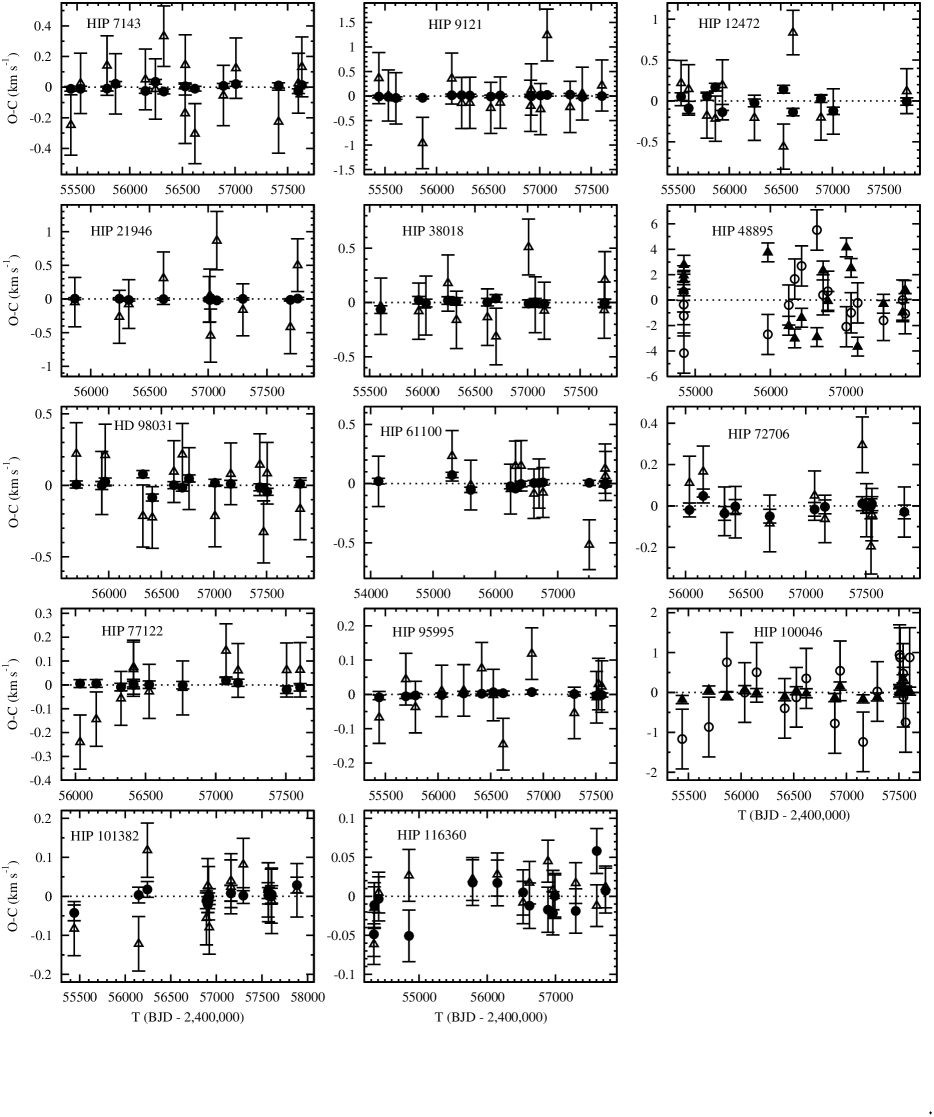
Figure 2: The residuals of the RVs obtained from todmor for the 14 SB2s. The circles refer to the primary component, and the triangles to the secondary component. For readability, the residuals of the most accurate RV measurements are in filled symbols.

5 Masses and parallaxes of HIP 61100, HIP 95995 and HIP 101382

When a visual orbit can be derived properly, an SB2 system with measured RV can be fully determined. Especially, the inclination can be evaluated and allows deriving the absolute mass of the system and of its components. Moreover with measurements independent of the Hipparcos 2 catalogue (van Leeuwen, 2007) it also allows verifying and correcting the Hippacos parallax taking into account the orbital motion. We found a visual orbit for 3 of the 14 SB2s presented in this paper; namely HIP 61100, HIP 95995 and HIP 101382.

5.1 HIP 61100

Our RV measurements were combined to the speckle and interferometric observations used by Schlieder et al. (2016), which are summarized in Table 6. The uncertainties of the interferometric measurements were corrected by 0.71 in order to obtain a visual orbit with a GOF $F_{2}=0$. These measurements are combined with our RV measurements and led to the orbital elements given in Table 7. The apparent orbit and its residuals are presented in Fig. 3. Our results are not really different from the preceding ones of Schlieder et al. (2016), but slightly more accurate, with masses ${\mathcal{M}}_{1}$=(0.834$\pm$0.017) ${\cal M}_{\odot}$ and ${\mathcal{M}}_{2}$=(0.640$\pm$0.011) ${\cal M}_{\odot}$, improving the mass measurement accuracy for these stars by a factor of 2.5 compared to Masda et al. (2016).

Our estimation of the parallax in Table 7, is more accurate, but compatible, with that given by the Hipparcos 2 catalogue: $\varpi=(39.84\pm 1.07)$ mas. However, this value was derived ignoring the orbital motion. A correction of the Hipparcos parallax was derived from the elements in Table 7 and from the residuals of the Hipparcos astrometric solution. The new value is then $\varpi=(40.75\pm 1.24)$ mas, in reasonable agreement with our result. No Tycho-Gaia Astrometric Solution (TGAS hereafter; see Michalik, Lindegren & Hobbs 2015; Gaia Collaboration, 2016) is available for this star, probably because of its orbital motion.

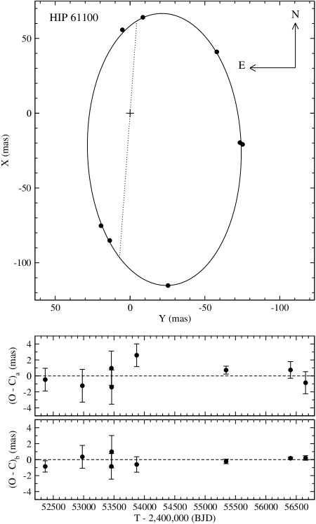
Figure 3: The visual part of the combined orbit of HIP 61100.Upper panel: the visual orbit; the circles are the positions from Table 8; the node line is in dashes. Middle panel: the residuals along the semi-major axis of the error ellipsoid. Lower panel: the residuals along the semi-minor axis of the error ellipsoid.

Table 6: The interferometric measurements of HIP 61100, taken from Schlieder et al. (2016) and adapted to our purpose. $X$ is oriented to North and $Y$ to East. $\sigma_{a}$ and $\sigma_{b}$ are the semi-major axis and the semi-minor axis of the ellipsoid error, respectively; they are corrected as explained in the text. $\theta_{a}$ is the position angle of the major axis of the ellipsoid error. $X$, $Y$ and $\theta_{a}$ are for equinox 2000.

$T$-2,400,000	$X$	$Y$	$\sigma_{a}$	$\sigma_{b}$	$\theta_{a}$
(BJD)	(mas)	(mas)	(mas)	(mas)	(o)
52367.9a	41.031	-57.944	1.425	0.706	125.3
52978.4	-115.245	-25.349	2.053	1.425	102.4
53456.7	-19.661	-73.413	2.138	1.604	75.0
53460.6	-20.835	-75.166	2.138	2.031	74.5
53872.8	55.760	5.181	1.425	0.969	5.3
55344.1	-75.230	19.436	0.499	0.285	165.5
56405.2	64.134	-8.537	1.041	0.143	82.4
56653.2a	-85.120	13.605	1.390	0.285	80.9

5.2 HIP 95995

This star is the close visual binary MCA 56. Masda et al. (2016) combined RV measurements and the interferometric measurements provided by the Fourth Catalog of Interferometric Measurements of Binary Stars (Third catalogue: Hartkopf et al., 2001) to derive the masses of the components: ${\cal M}_{1}$=(0.89$\pm$0.08) ${\cal M}_{\odot}$ and ${\cal M}_{2}$=(0.83$\pm$0.07) ${\cal M}_{\odot}$. We found that the less accurate measurements in the “Fourth Catalog” were also the less reliable ones, since their errors are much larger than their uncertainties; therefore, we derived the visual orbit taking into account only the measurements with uncertainties smaller than 2 mas. These measurements are presented in Table 8. We applied to these uncertainties a correcting factor of 0.81 in order to get the apparent orbit with the GOF $F_{2}=0$. The combination of the relative positions with our RVs leads to the parameters in Table 7. The apparent orbit and its residuals are presented in Fig. 4. We found the masses ${\cal M}_{1}$=(0.833$\pm$0.031) ${\cal M}_{\odot}$ and ${\cal M}_{2}$=(0.812$\pm$0.030) ${\cal M}_{\odot}$

We found the parallax $\varpi=(56.10\pm 0.81)$ mas, which is slightly different from that given in the Hipparcos 2 catalogue: $\varpi=(58.96\pm 0.65)$ mas. This is due to the orbital motion with a period close to one year: Correcting the Hipparcos parallax for this motion leads to $\varpi=(57.15\pm 0.31)$ mas, in acceptable agreement with our result. The parallax from TGAS (Michalik et al., 2015; Gaia Collaboration, 2016) is $\varpi=(58.37\pm 0.54)$ mas; the difference probably comes from the fact that the orbital motion was ignored in the calculation of TGAS.

Table 7: The combined VB+SB2 elements of HIP 61100, HIP 95995 and HIP 101382. For HIP 61100 and HIP 95995, the elements are derived from a combined VB+SB2 solution. For consistency with the SB orbits and with the forthcoming astrometric orbit, $\omega$ refer to the motion of the primary component.

	HIP 61100	HIP 95995	HIP 101382
$P$ (days)	1285.31 $\pm$ 0.27	494.307 $\pm$ 0.012	57.32176 $\pm$ 0.00010a
$T_{0}$ (BJD-2400000)	56492.13 $\pm$ 0.35	56549.505 $\pm$ 0.043	56627.3786 $\pm$ 0.0075a
$e$	0.51130 $\pm$ 0.00093	0.38933 $\pm$ 0.00029	0.43503 $\pm$ 0.00036a
$V_{0}$ (km s-1)	-9.7113 $\pm$ 0.0096	11.8932 $\pm$ 0.0018	-5.4108 $\pm$ 0.0057a
$\omega_{1}$ (o)	244.50 $\pm$ 0.16	180.325 $\pm$ 0.041	357.195 $\pm$ 0.064a
$\Omega$(o; eq. 2000)	355.83 $\pm$ 0.24	245.72 $\pm$ 0.13	334.960 $\pm$ 0.070b
$i$ (o)	58.63 $\pm$ 0.46	146.15 $\pm$ 0.46	99.364 $\pm$ 0.080b
$a$ (mas)	102.19	81.03	15.378 $\pm$ 0.027b
${\cal M}_{1}$ (${\cal M}_{\odot}$)	0.834 $\pm$ 0.017	0.833 $\pm$ 0.031	0.8420 $\pm$ 0.0014
${\cal M}_{2}$ (${\cal M}_{\odot}$)	0.640 $\pm$ 0.011	0.812 $\pm$ 0.030	0.66201 $\pm$ 0.00076
$\varpi$ (mas)	38.82 $\pm$ 0.23	56.10 $\pm$ 0.81	46.131 $\pm$ 0.084
$d_{2-1}$ (km s-1)	0.097 $\pm$ 0.064	0.112 $\pm$ 0.021	0.187 $\pm$ 0.020a
$\sigma_{(o-c)\;VB}$ (mas)	1.04	0.673	-
$\sigma_{(o-c)\;RV}$ (km s-1)	0.019, 0.202	0.0049, 0.066	0.017, 0.063a
$M_{A}$ (mag)	4.06 $\pm$ 0.25d	5.98 $\pm$ 0.02e	$\ldots$
$M_{B}$ (mag)	4.77 $\pm$ 0.27d	6.24 $\pm$ 0.03e	$\ldots$
$Y$	$0.245-0.27$	$0.245-0.279$	$\ldots$
age (Gyr)	0.4c	$2.2-7.9$	$\ldots$
${\rm[Fe/H]}$ (dex)	-0.17	-0.33$~{}-~{}$-0.17	$\ldots$

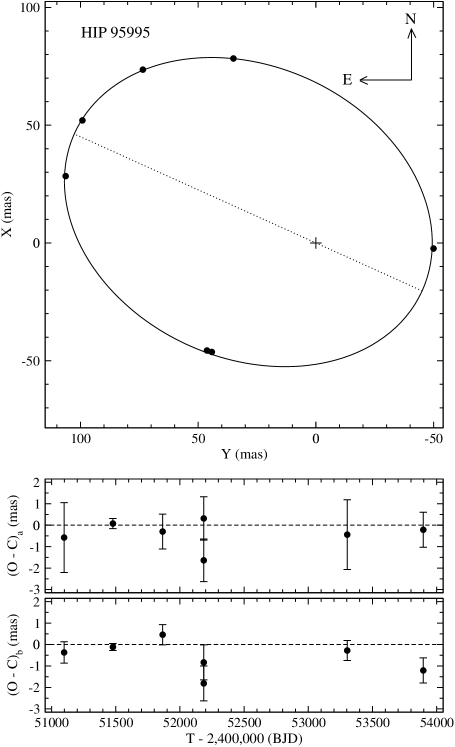
Figure 4: The visual part of the combined orbit of HIP 95995.Upper panel: the visual orbit; the circles are the positions from Table 8; the node line is in dashes. Middle panel: the residuals along the semi-major axis of the error ellipsoid. Lower panel: the residuals along the semi-minor axis of the error ellipsoid.

Table 8: Same as Table 6, but for HIP 95995. Only the positions more accurate than 2 mas are selected from the Fourth Catalogue of Interferometric Measurements of Binary Stars.

$T$-2,400,000	$X$	$Y$	$\sigma_{a}$	$\sigma_{b}$	$\theta_{a}$
(BJD)	(mas)	(mas)	(mas)	(mas)	(o)
51097.8	-2.366	-49.944	1.628	0.497	87.3
51478.0	78.322	35.032	0.236	0.163	114.1
51865.3	52.047	99.172	0.814	0.472	62.3
52185.5	-46.283	44.203	0.993	0.814	46.3
52185.5	-45.654	46.268	1.009	0.814	44.6
53303.2	28.382	106.275	1.628	0.464	75.0
53896.0	73.586	73.492	0.814	0.586	44.9

5.3 HIP 101382

For this system, Torres et al. (2002) already derived the orbital elements from the combination of observations made at the Palomar Testbed Interferometer, with RV measurements. Unfortunately, they did not provide the positions of the secondary component with respect to the primary, so we cannot compute a combined orbit as for the two preceding binaries. However, comparing the elements of their “full fit” with those derived from our RVs, it appears that, expressed in unit of uncertainties, the discrepancies for period, periastron epoch, eccentricity and periastron longitude are -0.41, 0.91, 1.81 and 0.69 respectively. These values are all between -2 and +2, indicating a nice agreement between their elements and our solutions. With the inclination derived from their ”full fit”, we found the new masses: ${\cal M}_{1}$=(0.8420$\pm$0.0014) ${\cal M}_{\odot}$ and ${\cal M}_{2}$=(0.66201$\pm$0.00076) ${\cal M}_{\odot}$, improving the accuracy on these masses by a factor of 10 compared to Torres et al. (2002).

Moreover, we evaluated a new measurement of the parallax $\varpi=(46.131\pm 0.084)$ mas. For comparison, the Hipparcos 2 catalogue gives $(45.35\pm 0.43)$ mas, which becomes $(45.31\pm 0.44)$ mas when our orbital elements are applied to the residuals of the Hipparcos astrometric solution. The Hipparcos 2 parallax is thus marginally compatible with ours, although slightly underestimated. The parallax from TGAS (Michalik et al., 2015; Gaia Collaboration, 2016) is $\varpi=(46.61\pm 0.83)$ mas, in good agreement with our result, although the orbital motion was not taken into account in the calculation.

6 Initial stellar parameters of HIP 61100 and HIP 95995

Having derived very accurate masses for HIP 61100 and HIP 95995 allowed us to characterize the two components of these binaries in terms of initial helium content and age. For that purpose, we modeled the two components following the stellar model optimisation method described in Lebreton & Goupil (2014). We adopted the reference set of stellar input physics described in that paper and the Cesam2k stellar evolution code (Morel & Lebreton, 2008). The observational constraints considered for the models are the masses of the two components herebefore determined, their effective temperatures and luminosities, and the present metallicity of the primary component. We point out that we decided not to model HIP 101382 because this binary system is enriched in $\alpha$-elements, with [$\alpha\text{/Fe}$]=$0.36$ (Torres et al., 2002). As discussed by Torres et al. (2002), a proper modeling would require to calculate new opacity tables which is beyond the scope of the present paper.

In support of the previous estimation of stellar parameters given in Table 2, we used the code iSpec (Blanco-Cuaresma et al., 2014) to verify the primary stellar parameters. Results for HIP 61100 and HIP 95995 are discussed below and appended to Table 7.

6.1 HIP 61100

To derive the luminosities of the components, we proceeded as follows. First, we used the system K band magnitude, $K$=5.662$\pm$0.020 from 2MASS (Cutri et al., 2003), the magnitude difference of the two components in the K band, $\Delta K$=0.71$\pm$0.02 (Schlieder et al., 2014), and the spectroscopic parallax derived in the present study. We obtained the absolute magnitudes $M_{K,A}$=4.06$\pm$0.25 and $M_{K,B}$=4.77$\pm$0.27 mag. Then, in the calculation of the stellar models, we derived the luminosity using the bolometric corrections $BC_{K}(T_{\mathrm{eff}},\log g,\mathrm{[Fe/H]})$ of Casagrande & VandenBerg (2014).

The iSpec derivation gave $T_{\text{eff}}$=5049$\pm$43 K, $\log g$=4.52$\pm$0.15 dex, and [Fe/H]=-0.13$\pm$0.10, as consistent with what derived in Table 2. Therefore, we constrained the stellar models with the effective temperatures of Table 2. The choice of the metallicity is more delicate. We therefore considered three possible values of the metallicity ($\mathrm{[Fe/H]}$=-0.13, -0.18, -0.33 dex) covering the range reported in the literature displayed in the SIMBAD database (Wenger et al. 2000)..

We further assumed that the stars have a common origin and therefore share the same initial metallicity, helium abundance and age. Their initial helium abundance in mass fraction should be higher than the primordial value $Y_{p}$ ​$\sim$0.245 (see e.g. Peimbert, Peimbert, & Luridiana, 2016; Izotov, Thuan, & Guseva, 2014). Furthermore, according to King et al. (2003), the system is a bona-fide member of the UMA Group nucleus. Therefore, we assumed that the common age of the components is 400 Myr, i.e. the age of the UMa group (Jones et al., 2015).

The model optimisation provides the initial helium abundance for each star. The results are shown in Fig. 5.

We first note that low values of the metallicity ($\mathrm{[Fe/H]}$=$-0.33$ dex) can be excluded because they would lead to a sub-primordial initial helium abundance of the system. On the other hand, considering also the constraint that the two components have the same initial helium abundance, we find good compatibility with models on the higher metallicity case, with $\mathrm{[Fe/H]}\sim-0.15$, provided that the primary mass is on the lower bound and secondary mass on the upper bound of their confidence interval. Finally, we also explored the possibility that the stars have an age of 500 Myr, as assumed by Schlieder et al. (2016) but did not find any satisfactory solution with the subsolar $\mathrm{[Fe/H]}$ values considered here.

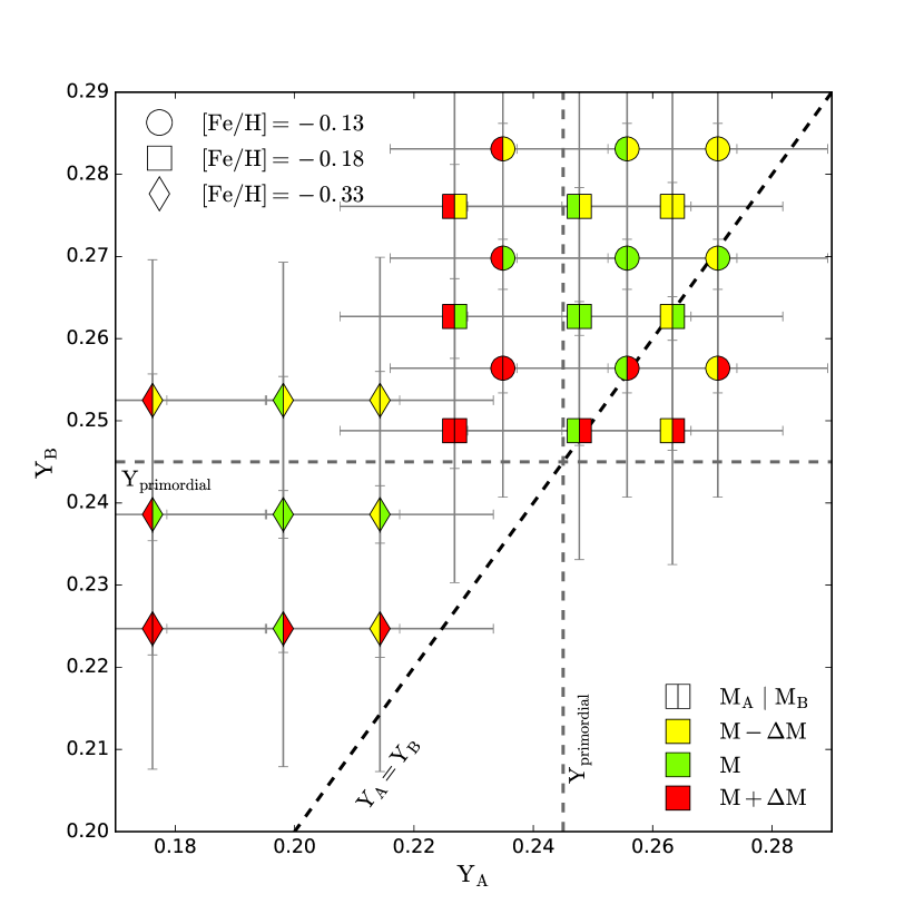
Figure 5: Initial He abundance of the primary and secondary components of HIP 61100 inferred from different sets of optimized models. Different symbols correspond to different assumptions on the measured metallicity [Fe/H], as found for the same star HIP 61100A in the literature. Independent iSpec derivation of HIP 61100 metallicity gives [Fe/H]=-0.13$\pm$0.10 dex. Each symbol is separated in two, primary star on the left side and secondary on the right. Each mass is varied on its confidence interval, leading to different estimation of the He abundance.

6.2 HIP 95995

To derive the luminosities, we took the parallax derived here, the system V band magnitude ($V$=6.607$\pm$0.010) from Tycho 2 (Høg et al., 2000), and the magnitude difference of the two components in the $V$ band ($\Delta V$=0.26$\pm$0.03) which we calculated as the mean of interferometric values listed in Table 2 of Masda et al. (2016), but keeping the values with given error bars only. We obtained the absolute magnitudes $M_{V,A}$=5.98$\pm$0.02 and $M_{V,B}$=6.24$\pm$0.03 mag. Then, we applied the bolometric corrections of Casagrande & VandenBerg (2014). We did not include extinction, since it is usually expected to be very small for a star at less than 20 pc.

The primary stellar parameters derived from iSpec are $T_{\mathrm{eff}}$=4972$\pm$32 K and $\mathrm{[Fe/H]}$=-0.45$\pm$0.27, in reasonable agreement with those derived in Table 2. Therefore, we constrained the stellar models with the effective temperatures of Table 2. Since Casagrande et al. (2011) rather derived $\mathrm{[Fe/H]}$=-0.17, we performed two sets of models, one with the metallicity determined here ($\mathrm{[Fe/H]}$=-0.33) and one with $\mathrm{[Fe/H]}$=-0.17.

In the case of HIP 95995, we do not have constraints on the age. However, the star is classified as inactive by Gray et al. (2003) which is not in favor of young ages. Moreover, Casagrande et al. (2011) gives a rough estimation of the age of this system, 13.8$\pm$6 Gyr.

To model the system, we first optimized models of the primary component, adjusting the age, initial helium abundance and metallicity; and then we searched for a model of the secondary component by fixing its age and initial composition equal to those of the primary. Unfortunately, despite the improvement on the mass, the stellar model of HIP 95995 remains rather poorly constrained, due to possible misestimation of the secondary’s stellar parameters. We thus eventually discarded the secondary’s constraint and only considered the contribution of the primary in the following.

No acceptable solution (Y$>$Y${}_{\text{primordial}}$ and age$>$1 Gyr) is found for the upper part of the mass confidence interval (${\cal M}_{A}$ ​$>$0.833 ${\cal M}_{\odot}$), and decreasing or increasing the metallicity still leads to reject the models. At ${\cal M}_{A}$=0.833 ${\cal M}_{\odot}$, the best models stand around $\mathrm{[Fe/H]}$=-0.17; they lead to an age range $\sim$2.2-5.3 Gyr and initial helium abundance $Y_{0}$=0.250-0.265. Finally, for ${\cal M}_{A}$ ​$<$0.833 ${\cal M}_{\odot}$, the most suitable models have ages in the range 2.4-7.9 Gyr, initial helium abundance in the range 0.245-0.279, and metallicity between -0.17 and -0.33.

7 Summary and conclusion

Thanks to new SOPHIE spectra of 14 SB2s, four of which are newly identified SB2 (paper I), and the use of the todmor code, we derived new better accurate orbital solutions to the RV measurements of these binaries. The projected masses ${\cal M}\sin^{3}i$ were calculated for all 14 SB2s, with an average accuracy of 1.0$\pm$0.2 %, with extreme cases such as the rapid rotator HIP 48898 with $\sigma({\cal M}\sin^{3}i)$ ​$\sim$4 %, or HIP 101382 with $\sigma({\cal M}\sin^{3}i)$ ​$\sim$0.12 %.

For HIP 61100, HIP 95995 and HIP 101382, archival interferometric measurements allowed us to fully constraint the systems and derive masses for components (A,B) with accuracies respectively (2.0, 1.7) %, (3.7, 3.7) %, and (0.2, 0.1) %. The stellar evolution code Cesam2k (Morel & Lebreton, 2008) applied to HIP 61100 and HIP 95995, led to constrain their age, metallicity and initial helium content. HIP 61100 was found slightly overabundant in He with respect to primordial helium abundance, with $\mathrm{[Fe/H]}\sim-0.15$ dex and an age close to 400 Myr, while HIP 95995 was harder to constrain, assuming a relatively old star with age$>$1 Gyr, and using only primary star’s mass and stellar parameters, led to a possible overabundance in He, with -0.33$<$[Fe/H]$<$0.17.

Although we could not calculate stellar evolution models of HIP 101382, the masses of the SB2 components that we derived reached the level of 0.1 % accuracy. In the future, this star will likely become a reference for validating masses derived from Gaia.

Added to the systems already published in papers II and III, we have now 6 binaries observed with SOPHIE and interferometric instruments which may be used to verify the masses that will be derived from Gaia. This number will continue to increase until the completion of the programme.

References

- Angelov (1996) Angelov T., 1996, BABel, 154, 13
- Blanco-Cuaresma et al. (2014) Blanco-Cuaresma S., Soubiran C., Heiter U., Jofré P., 2014, A&A, 569, A111
- Carquillat, Griffin & Ginestet (1995) Carquillat J.-M., Griffin R.F., Ginestet N., 1995, A&AS 109, 173
- Casagrande et al. (2011) Casagrande L., Schönrich R., Asplund M., Cassisi S., Ramírez I., Meléndez J., Bensby T., Feltzing S., 2011, A&A, 530, A138
- Casagrande & VandenBerg (2014) Casagrande L., VandenBerg D. A., 2014, MNRAS, 444, 392
- Cutri et al. (2003) Cutri R. M., et al., 2003, tmc..book,
- Drake (1991) Drake J. J., 1991, MNRAS, 251, 369 et al.
- Duquennoy & Mayor (1988) Duquennoy A., Mayor M., 1988 A&A 195, 129
- Gaia Collaboration (2016) Gaia Collaboration, 2016 A&A 595, A2
- Goldberg et al. (2002) Goldberg D., Mazeh T., Latham D.W., Stefanik R.P., Carney B.W., Laird J.B., 2002, AJ, 124, 1132
- Gray et al. (2003) Gray R.O., Corbally C.J., Garrison R.F., McFadden M.T., Robinson P.E., 2003, AJ 126, 2048
- Griffin (2005a) Griffin R.F., 2005a, Observatory, 125, 134
- Griffin (2005b) Griffin R.F., 2005b, Observatory 125, 253
- Griffin (2005c) Griffin R.F., 2005c, Observatory 125, 367
- Griffin (2006) Griffin R.F., 2006, Observatory 126, 119
- Halbwachs et al. (2003) Halbwachs, J. L., Mayor, M., Udry, S., & Arenou, F. 2003, A&A, 397, 159
- Halbwachs, Mayor & Udry (2012) Halbwachs J.-L., Mayor M., Udry S., 2012, MNRAS 422, 14
- Halbwachs et al. (2014) Halbwachs J.L., Arenou F., Pourbaix D., Famaey B., Guillout P. et al., 2014, MNRAS 445, 2371 (paper I)
- Halbwachs et al. (2016) Halbwachs J.L., Boffin H.M.J., Le Bouquin J.-B., Kiefer F., Famaey B. et al., 2016, MNRAS 455, 3303 (paper II)
- Hartkopf et al. (2001) Hartkopf W.I., McAlister H.A, Mason B.D., 2001, AJ 122, 3480
- Hodgson et al. (1985) Hodgson R.M., Bailey D.G., Naylor M.J., Ng A.L.M., McNeil S.J., 1985, Image Vision Comput., 3(1), 4-14
- Høg et al. (2000) Høg E., Fabricius C., Makarov V.V. et al., 2000 A&A 355, L27
- Husser et al. (2013) Husser T.-O. et al., 2013, A&A, 553, A6
- Izotov, Thuan, & Guseva (2014) Izotov Y. I., Thuan T. X., Guseva N. G., 2014, MNRAS, 445, 778
- Jones et al. (2015) Jones J., et al., 2015, ApJ, 813, 58
- Katoh et al. (2013) Katoh N., Itoh Y., Toyota E., Sato B., 2013, AJ 145, 41
- Kiefer et al. (2016) Kiefer, F., Halbwachs, J.-L., Arenou, F., et al. 2016, MNRAS, 458, 3272 (paper III)
- King et al. (2003) King J. R., Villarreal A. R., Soderblom D. R., Gulliver A. F., Adelman S. J., 2003, AJ, 125, 1980
- Lebreton & Goupil (2014) Lebreton Y., Goupil M. J., 2014, A&A, 569, A21
- Masda et al. (2016) Masda S.G., Al-Wardat M.A., Neuhäuser R., Al-Naimiy H.M., 2016, Research in A.A., 16, 112
- Mashonkina et al. (2007) Mashonkina, L., Korn, A. J., Przybilla, N., 2007, A&A, 461, 261-275
- Massarotti et al. (2008) Massarotti A., Latham D.W., Stefanik R.P., Fogel J., 2008, AJ, 135, 209
- Michalik et al. (2015) Michalik D., Lindegren L., Hobbs D., 2015, A&A, 574, A115
- Morel & Lebreton (2008) Morel P., Lebreton Y., 2008, Ap&SS, 316, 61
- Peimbert, Peimbert, & Luridiana (2016) Peimbert A., Peimbert M., Luridiana V., 2016, RMxAA, 52, 419
- Perruchot et al. (2008) Perruchot S., et al., 2008, SPIE, 7014, 70140J
- Pourbaix (2000) Pourbaix D., 2000, A&AS 145, 215
- Pourbaix et al. (2004) Pourbaix D., Tokovinin A. A., Batten A. H., Fekel F. C., Hartkopf W. I., Levato H., Morell N. I., Torres G., Udry S., 2004, A&A, 424, 727
- Schlieder et al. (2014) Schlieder J. E., et al., 2014, ApJ, 783, 27
- Schlieder et al. (2016) Schlieder J.E., Skemer A.J., Maire A.-L., Desidera S., Hinz P. et al., 2016, AJ 818, 1
- Torres et al. (2002) Torres G., Boden A.F., Latham D.W., Pan M., Stefanik R.P., 2002, AJ 124, 1716
- Torres et al. (2012) Torres G., Fischer D. A., Sozzetti A., Buchhave L. A., Winn J. N., Holman M. J., Carter J. A., 2012, ApJ, 757, 161
- van Leeuwen (2007) van Leeuwen F., 2007, A&A 474, 653
- Zucker & Mazeh (1994) Zucker S., Mazeh, T., 1994, ApJ, 420, 806
- Zucker et al. (2004) Zucker S., Mazeh T., Santos N. C., Udry S., Mayor M., 2004, A&A, 426, 695