Time-Resolved Two Million Year Old Supernova Activity Discovered in the Earth’s Microfossil Record

Abstract

Massive stars ($M\gtrsim 10\leavevmode\nobreak\ M_{\odot}$), which terminate their evolution as core collapse supernovae, are theoretically predicted to eject $>10^{-5}M_{\odot}$ of the radioisotope ⁶⁰Fe (half-life $2.61$ Ma). If such an event occurs sufficiently close to our solar system, traces of the supernova debris could be deposited on Earth. Herein, we report a time-resolved ⁶⁰Fe signal residing, at least partially, in a biogenic reservoir. Using accelerator mass spectrometry, this signal was found through the direct detection of live ⁶⁰Fe atoms contained within secondary iron-oxides, among which are magnetofossils; the fossilized chains of magnetite crystals produced by magnetotactic bacteria. The magnetofossils were chemically extracted from two Pacific Ocean sediment drill cores. Our results show that the ⁶⁰Fe signal onset occurs around $2.6-2.8$ Ma, near the lower Pleistocene boundary, terminates around $1.7$ Ma, and peaks at about $2.2$ Ma.

This manuscript was compiled on

-2pt

The isotope ⁶⁰Fe is mostly produced during the evolution of massive stars ($M\gtrsim 10\leavevmode\nobreak\ M_{\odot}$) in two steps along the course of their evolution. In the first step, during their quiescent helium and carbon shell burning phases, ⁶⁰Fe is synthesized at the base of these shells by a slow neutron capture process on pre-existing stable seed nuclei, mostly by two successive neutron captures starting on stable ⁵⁸Fe [1]. In the second step, shock heating within the carbon-shell, driven by the passage of the supernova (SN) blast wave, allows for the synthesis of a modest amount of ⁶⁰Fe just prior to the subsequent disruption of the star and the concomitant explosive ejection of these shell mass zones, and the ⁶⁰Fe within them, into the interstellar medium. The subsequent beta-decay of ⁶⁰Fe, which has a half-life of $t_{1/2}=(2.61\pm 0.04)\leavevmode\nobreak\$Ma [weighted average of refs. 2, 3], gives rise to two characteristic gamma-ray lines, which have been detected in the central part of the galactic plane [4], known to be a site of massive stars, confirming the association of ⁶⁰Fe formation with regions of ongoing massive star nucleosynthesis.

If a core-collapse supernova (CCSN) occurs sufficiently close to our solar system, part of the ejected matter should arrive in our solar system. The best candidate mechanism for overcoming the solar wind pressure and penetrating to the Earth’s orbit is dust transport [5, 6]. Recent investigations with far-infrared to sub-millimeter telescopes suggest that CCSN ejecta are efficient dust sources [7]. For instance, copious amounts of dust with a large mass fraction contained in grains of above $0.1\leavevmode\nobreak\ \mu$m size (and up to $4.2\leavevmode\nobreak\ \mu$m) have recently been observed in the ejecta of supernova 2010jl [8]. During atmospheric entry, dust grains are expected to be partially or totally ablated, depending on composition, incident velocity, and angle of entry [9]. The ⁶⁰Fe released in the ablated fraction will enter the terrestrial iron cycle [10] and become deposited into geological reservoirs such as marine sediments.

An excess of ⁶⁰Fe was already observed in $\sim 2$ Ma old layers of a ferromanganese (FeMn) crust retrieved from the Pacific Ocean [5, 11, 12] and recently in lunar samples [13]. However, due to the slow growth rate of the FeMn crust, the ⁶⁰Fe signal had a poor temporal resolution. This ⁶⁰Fe has been attributed to a deposition of SN ejecta; though, this interpretation has been challenged by an alternate hypothesis attributing the ⁶⁰Fe excess to micrometeorites [14, and references therein]. An independent indication of a recent SN interaction with our solar system was recently deduced from the spectra of cosmic ray particles [15]. In our work herein, we aimed at the analysis of the entire temporal structure of the ⁶⁰Fe signature in terrestrial samples. This requires a geological reservoir with an excellent stratigraphic resolution, high ⁶⁰Fe sequestration and low Fe mobility, which preserves ⁶⁰Fe fluxes as they were (or nearly so) at the time of deposition, apart from radioactive decay. Both conditions were fulfilled in the carefully selected marine sediments used in this study.

One particularly interesting mechanism by which Fe is sequestered within sediments is through biomineralization, e.g. by dissimilatory metal reducing bacteria (DMRB) [16], and by magnetotactic bacteria (MTB) [17]. MTB are single-cell prokaryotes, which produce intracellular chains of magnetite (Fe₃O₄) nanocrystals called magnetosomes [18, 19]. These bacteria achieve their highest population densities near the so-called oxic-anoxic transition zone [20], where the oxygen concentration drops, producing a well-defined redox boundary. In pelagic sediments, this boundary occurs within few centimeters below the sediment-water interface [21], forcing the MTB populations to move upwards as the sediment column grows, with dead cells being left behind. After decomposition of the dead cells, the magnetosomes remain embedded within the sediment bulk and are subsequently called magnetofossils [22].

The ablated Fe fraction of SN dust grains arriving in the oceans is expected to undergo dissolution and re-precipitation upon reaching the sediment in the form of nano-minerals, such as poorly crystalline ferric hydroxides [10]. The poor solubility of Fe(III) minerals at circumneutral pH values ($\sim 0.1$ nmol/L) means that Fe is hardly mobilizable under oxygenated conditions. Many microorganisms, including DMRB and MTB, get around this problem by excreting organic compounds known as siderophores, which specifically complex Fe(III). DMRB reduce Fe(III) to highly soluble Fe(II), which in turn leads to the precipitation of new minerals, among which is magnetite (Fe₃O₄) [16]. Other bacteria perform Fe(II) oxidation [23]. The Fe uptake capability of DMRB from particulate sources depends on the type of source mineral and particle size. Poorly crystalline hydroxides, such as ferrihydrite (FeOOH), are preferred over goethite ($\alpha$-FeOOH) and hematite ($\alpha$-Fe₂O₃), and Fe reduction rates are proportional to the specific surface area of particles [24, 25, 26]. In particular, surface normalized bacterial Fe-reducing reaction rates are $\sim 1.5-2$ orders faster [26] for nano-sized ferrihydrite particles as compared to grains with sizes comparable to bulk detrital grains. The Fe uptake capability of MTB has been investigated less extensively. Common constituents of the DMRB iron metabolism, such as genes for ferrous and ferric iron uptake, siderophore synthesis, iron reductases, as well as iron-regulatory elements, are present in MTB [19]. MTB are therefore able to take up ferric and ferrous iron from various sources [27] with similar capabilities as for DMRB. This is also supported by the fact that MTB are the main source of one reduction product – magnetite – in many types of sediments [28, 29, 30, 31]. The combination of Fe reducing and oxidizing reactions supports the Fe cycle in sediments, yielding ultrafine ($<100$ nm) secondary Fe minerals [32, 33] (see Supporting Information).

MTB extant at the time of supernova ⁶⁰Fe input to the ocean floor are expected, therefore, to have incorporated ⁶⁰Fe into their magnetosomes, biogenically recording the supernova signal. Unlike other Fe minerals and biomineralization products, magnetofossils have unique magnetic signatures enabling their detection down to mass concentrations in sediment of the order of few ppm [29]. As an essential point for this work, magnetofossil preservation ensures that the ⁶⁰Fe signal is not altered, because the very existence of these microfossils means that post-depositional Fe mobilization through reductive diagenesis [34, 28] did not occur.

In general, Fe(III) sources accessible to bacterial reduction can be extracted with buffered solutions of reducing agents such as citrate-bicarbonate-dithionite (CBD) and, to a lesser extent, ammonium oxalate [35]. The CBD protocol [36] has been specially conceived to selectively dissolve fine-grained ($<200\leavevmode\nobreak\$nm) secondary oxides in soils, but not larger particles of lithogenic origin [37, 38] (see Supporting Information). Therefore, CBD can be used to selectively extract Fe from magnetofossils and other secondary minerals along with ⁶⁰Fe, thereby minimizing any dilution from large-grained, ⁶⁰Fe-free primary mineral phases.

Materials and Methods

In our search for a biogenic supernova signal, we selected two sediment cores, core 848 and core 851, from the equatorial Pacific (2°59.6’S, 110°29’W, 3.87 km water depth), recovered by the Ocean Drilling Program during Leg 138 [39]. The sediment of both cores is a pelagic carbonate (60–80% CaCO₃, 20–30% SiO₂) with a total iron content of 1.5–3.5 wt% [40]. Both cores are characterized by an excellent bio- and magnetostratigraphic record and almost constant sedimentation rates of ($6.1\leavevmode\nobreak\ \pm\leavevmode\nobreak\ 0.1$) m/Ma and ($19.3\leavevmode\nobreak\ \pm\leavevmode\nobreak\ 0.2$) m/Ma for core 848 and 851, respectively, over the 1.7-2.7 Ma age range of interest [41], as shown in Fig. 1.

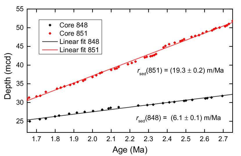
Figure 1: Age model data [taken from 41] of ODP drill cores 848 and 851 with linear fits overlaid. The X-axis represents the depth in the respective drill cores in meters core depth (mcd). The slopes of the fits yield sedimentation rates as shown. No significant departure from linearity is observed across the displayed time range, indicating both cores had constant sedimentation rates. The errors represent 1-$\sigma$ standard deviations.

The presence of magnetofossils in these cores was confirmed by electron microscopy and magnetic analysis techniques based on first-order reversal-curve measurements [42, 29] (see Supporting Information). The average magnetofossil Fe concentration over the 1.7–3.4 Ma interval was determined to be 25–30 $\mu$g/g for core 848, and 15–20 $\mu$g/g for core 851, respectively. Along with a constant sedimentation rate (Fig.1) and sediment composition [43], the lack of significant magnetofossil concentration variations, both absolute and relative to other magnetic Fe minerals, indicates that the depositional environment was stable during the period of time period under investigation. An additional confirmation of stable sedimentation conditions was obtained by measurements of the ¹⁰Be/⁹Be ratio in representative samples of core 851, which show no significant deviation from exponential radioactive decay (see Supporting Information).

In order to maximize the ⁶⁰Fe/Fe atom ratio, a highly selective version of the CBD procedure [36] was developed (see Supporting Information). This is a very mild chemical leaching technique, able to completely dissolve secondary iron oxides such as magnetofossils, while leaving larger grains, which may not contain ⁶⁰Fe, essentially intact [29]. At least 27% of the total Fe extracted with this technique is contained in magnetofossils [29], which therefore represent a significant contribution to the analyzed Fe pool. Even with this carefully designed extraction protocol, the expected ⁶⁰Fe concentrations are so low that the only viable measurement technique is ultra-sensitive AMS, which has been carried out at the GAMS (Gas-filled Analyzing Magnet System) setup [44] at the Maier-Leibnitz-Laboratory (MLL) in Garching (Germany) over several beamtimes. The MLL features a 14 MV MP Tandem accelerator with an energy stability of $\Delta E/E\approx 10^{-4}$. For AMS measurements of ⁶⁰Fe, the samples are prepared as Fe₂O₃ powder mixed 50/50 by volume with Ag powder (-120 mesh, Alfa Aesar, Lot Nr. J07W011), which is subsequently hammered into a 1.5 mm wide hole, drilled into a silver sample holder.

Fe was extracted as FeO^- from a single-cathode, cesium sputter ion source, and injected into the accelerator after a pre-acceleration to 178 keV. The tandem terminal voltage for the experiments described here was between 11 MV and 12 MV, which favored selection of the charge state 10⁺ for the radioisotope ⁶⁰Fe after passing through a 4 $\mu$m thick carbon stripper foil at the accelerator terminal. A charge state of 9⁺ was selected for the stable beam of ⁵⁴Fe, since it has nearly the same magnetic rigidity as ⁶⁰Fe¹⁰⁺ at the same terminal voltage. After acceleration to 110–130 MeV (depending on the available terminal voltage), the ions exit the accelerator and pass another dipole magnet for selection of the correct magnetic rigidity, as well as two Wien-velocity filters. Finally, the ions are directed towards the dedicated GAMS (Gas-filled Analyzing Magnet System) beamline by way of a switching magnet. Through use of the GAMS magnet, the challenging suppression of the stable isobar ⁶⁰Ni is achieved.

The GAMS magnet chamber is filled with 4–7 mbar of N₂ gas. Through electron exchange reactions with the N₂ gas, each ion species adopts an equilibrium charge state which depends on its atomic number $Z$. Thus, isobars will be forced on different trajectories if a magnetic field is applied. Since ⁶⁰Fe and ⁶⁰Ni have $\Delta Z=2$, their trajectories on the exit-side of the magnet can be spatially separated by 10 cm. The GAMS magnetic field can then be adjusted to make ⁶⁰Fe to reach the particle identification detector, while most ⁶⁰Ni is blocked using a suitable aperture in front of the detector entrance. The detector itself is an ionization chamber featuring a Frisch-grid and a five-fold split anode and is filled with $30-50$ mbar isobutane as counting gas. Individual ⁶⁰Fe ions can thus be identified by their energy deposition (Bragg-curve), which is described in more detail in the Supporting Information.

For measurements of the atom ratio ⁶⁰Fe/Fe, the stable beam of ⁵⁴Fe⁹⁺ is tuned into a Faraday cup in front of the GAMS, where the typical current is $30-150\leavevmode\nobreak\$enA (sample dependent). Then, the terminal voltage and the injector magnet are switched to allow ⁶⁰Fe¹⁰⁺ to pass and the Faraday cup is retracted. ⁶⁰Fe ions are then individually identified and counted in the ionization chamber, while the ⁶⁰Ni background count-rate is only about $10-100\leavevmode\nobreak\$Hz. In this manner, a highly selective discrimination of ⁶⁰Fe against ⁶⁰Ni and other background sources is achieved, as demonstrated by the extremely low blank levels obtained with different blank materials, such as processing blanks and environmental samples. The concentration of ⁶⁰Fe/Fe is calculated from the number of ⁶⁰Fe events counted by the detector, the measurement time, and the average current of ⁵⁴Fe⁹⁺ in front of the GAMS. The transmission between the Faraday cup and the detector is canceled out by relating the result to the known concentration of a standard sample, which is measured periodically during a beamtime. For this work, the standard sample PSI-12, with a concentration ${}^{60}\text{Fe/Fe}=(1.25\pm 0.06)\times 10^{-12}$, was used (see Supporting Information). The transmission efficiency of the entire system (including ion source yield, stripping yield, ion-optical transmissions, and software cuts) during ⁶⁰Fe measurements is in the range $(1-4)\times 10^{-4}$.

Results

A total of 111 sediment samples (67 from core 848 and 44 from core 851), each with a mass of $\sim 35\leavevmode\nobreak\$g, were treated with the CBD protocol, yielding $\sim 5$ mg AMS samples consisting of Fe₂O₃. Each AMS sample was measured for an average of 4 hours until the sample material was exhausted, yielding one ⁶⁰Fe event on average and a total of 86 events integrated over both cores (42 in core 848, 47 in core 851). Thus, several AMS samples have been grouped together to increase counting statistics, as displayed in Fig. 2. Owing to the availability of several near-surface ($0-1$ Ma) and very deep ($7-8$ Ma) samples in core 848, the presence of a distinct ⁶⁰Fe signal could be clearly identified (Fig. 2A). The data is complemented by the observation of a similar signal in core 851 (Fig. 2B), which is characterized by a $\sim$ 1.5 times lower ⁶⁰Fe/Fe ratio. The onset of the ⁶⁰Fe signal occurs at $(2.7\pm 0.1)$ Ma and is centered at ($2.2\pm 0.1$) Ma. The signal termination is not as clear, since it remains slightly above the 1-$\sigma$ blank level until around 1.5 Ma, according to the data grouping used in Fig. 2A. A detailed analysis averaging over both sediment cores and several data groupings yields a more conservative estimate for the termination time of ($1.7\pm 0.2$) Ma. This results in a ($1.0\pm 0.3$) Ma long exposure of the Earth to the influx of ⁶⁰Fe.

An overview of the collected AMS data split into three age regions ($<1.8$ Ma, $1.8-2.6$ Ma, $>2.6$ Ma) is shown in Tab. LABEL:Tab:1. An estimate for the significance of the ⁶⁰Fe signal in the peak region can be obtained by applying the procedure suggested by ref. [45] for the superposition of two Poisson processes (i.e. signal and background). As a control region (no expected signal), we selected (1) the processing blank and, for comparison, (2) the $<1.8$ Ma age interval of each respective sediment core. The second choice is rather conservative, since this overestimates the background signal. In the case of (1), the procedure yields a significance (in multiples of $\sigma$) of 5.2 and 3.9 (for core 848 and 851, respectively). In the case of (2) these values become 7.2 and 2.0. The significance for core 851 is low in the case of (2), since only little data was collected in the control region.

A useful measure for the intensity of the total ⁶⁰Fe exposure is given by the terrestrial ($\Phi_{\text{ter}}$) fluence of ⁶⁰Fe. $\Phi_{\text{ter}}$ represents the time-integrated, decay corrected flux of ⁶⁰Fe into a given terrestrial reservoir over the entire exposure time. In order to sum up the contributions of all sediment layers in the signal range, the following integral is computed to calculate the average concentration of ⁶⁰Fe/Fe in the signal range:

$$\overline{\mathcal{C}}=(t_{2}-t_{1})^{-1}\int_{t_{1}}^{t_{2}}\mathcal{C}(^{60}\text{Fe/Fe})\text{d}t$$ (1)

The average terrestrial ⁶⁰Fe fluence, $\Phi_{\text{ter}}$, is then given by

$$\Phi_{\text{ter}}=\overline{\mathcal{C}}\rho r_{\text{sed}}(t_{2}-t_{1})Y_{\text{CBD}}N_{\text{A}}/W_{\text{Fe}}$$ (2)

where $\rho$ is the dry sediment density, $r_{\text{sed}}$ is the sedimentation rate, $Y_{\text{CBD}}$ is the efficiency corrected CBD yield of extracted iron from per unit mass of dry sediment, $N_{\text{A}}$ is Avogadro’s number, and $W_{\text{Fe}}$ is the molecular weight of iron. Using $(t_{2}-t_{1})=(1.0\pm 0.3)$ Ma as a nominal signal duration results in a terrestrial fluence into our sediments of $\Phi_{\text{ter}}^{\text{848}}=(4.7\pm 1.6)\times 10^{5}$ at/cm² and $\Phi_{\text{ter}}^{\text{851}}=(8.8\pm 2.9)\times 10^{5}$ at/cm² for cores 848 and 851, respectively. The slightly different values and larger errors compared to Tab. 1 result from an averaging over different exposure times $(t_{2}-t_{1})$, whereas the fluences in Tab. 1 were calculated for a fixed $(t_{2}-t_{1})=0.8\leavevmode\nobreak\$Ma. For the following discussion, we use the error-weighted mean of the fluences determined in both sediment cores, which is $\Phi_{\text{ter}}^{\text{sed}}=(5.6\pm 1.4)\times 10^{5}$ at/cm².

In order to compare this result with the fluence obtained by ref. [11] for the Pacific Ocean FeMn crust, several correction factors must first be applied. Since those results were published, the half-life of ⁶⁰Fe has undergone a revision [2, 3]; the half-life of ¹⁰Be, which was used to convert the crust growth rate to geological time, has also been re-determined [46, 47]. A correction for the different ⁶⁰Fe standard samples used (which became available due to advanced cross-calibration measurements), must be taken into account. The resulting, decay corrected, terrestrial fluence derived from the FeMn crust now becomes $\Phi_{\text{ter}}^{\text{crust}}=(2.5\pm 1.3)\times 10^{6}$ at/cm², which is about a factor of $4-5$ higher than our result and does not take an uptake efficiency for Fe of the FeMn crust into account. Interestingly, another recently reported fluence value deduced from Indian Ocean sediments [48] ($\Phi_{\text{ter}}^{\text{ind}}=(35.4\pm 2.6)\times 10^{6}$ at/cm²) is 1-2 orders of magnitude higher than the value reported in this work. Possible explanations for such differences are (1) a non-uniform ⁶⁰Fe deposition at the respective locations of the geological reservoirs [see e.g. 49] and (2) a selective chemical Fe uptake from bottom water currents at certain locations leading to fluence values above those related to the depositional flux.

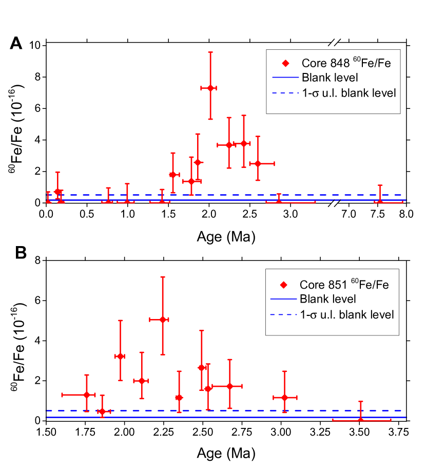
Figure 2: ⁶⁰Fe/Fe atom ratio determined in all sediment samples of core 848 (A) and 851 (B). Y-error bars indicate 1-$\sigma$ statistical uncertainties. The X-axes limits were chosen according to the availability of sample material, which also explains the broke X-axis in (A). X-error bars represent core depth of sample material used for each data point. Each data point contains 3-6 adjacent individual AMS samples grouped together. The blank level and its 1-$\sigma$ upper limit (u.l.) are shown for a chemical processing blank. Note that panel (A) has a broken time axis relative to panel (B).

Table 1: Summary of all ⁶⁰Fe data presented in this work. Lines indicate separation of the sediment cores into three intervals. The last line represents data obtained from processing blank material. The corrected (corr.) ⁶⁰Fe/Fe concentrations are corrected for radioactive decay and the blank level. All errors are given as 1-$\sigma$ uncertainties.

Sample	Age range	Number of	60Fe events	60Fe/Fe AMS	60Fe/Fe corr.	Deposition rate	Terrestrial fluence $\Phi_{\text{ter}}$
	(Ma)	samples		($\times 10^{-16}$)	($\times 10^{-16}$)	(at. 60Fe a-1 cm-2)	($10^{5}$ at.60Fe cm-2)
Core 848	$0.0-1.8$	$25$	$4$	$0.3^{+0.2}_{-0.1}$	$0.2^{+0.3}_{-0.2}$	$0.02^{+0.03}_{-0.02}$	$0.10^{+0.18}_{-0.10}$
Core 848	$1.8-2.6$	$27$	$38$	$4.3\pm 0.9$	$7.4\pm 1.2$	$0.50\pm 0.14$	$4.0\pm 1.0$
Core 848	$2.6-8.0$	$15$	$0$	$<0.3$	$<0.9$	$<0.06$	$<0.48$
Core 851	$1.6-1.8$	$3$	$2$	$1.6^{+1.8}_{-1.0}$	$2.4^{+2.9}_{-1.6}$	$0.47^{+0.56}_{-0.32}$	$3.4^{+4.5}_{-2.5}$
Core 851	$1.8-2.6$	$22$	$40$	$2.7\pm 0.4$	$4.6\pm 0.8$	$0.92\pm 0.23$	$7.5\pm 2.5$
Core 851	$2.6-3.7$	$19$	$5$	$1.1^{+0.6}_{-0.5}$	$2.2^{+1.4}_{-1.1}$	$0.44^{+0.26}_{-0.22}$	$3.5^{+2.0}_{-1.8}$
Blank		$18$	$1$	$0.2^{+0.3}_{-0.1}$

Conclusions

In summary, we have extracted magnetofossils and other iron-bearing secondary minerals from two Pacific Ocean sediment cores, 848 and 851 of the ODP Leg 138. Using AMS on samples derived from these mineral phases, we have detected a time-resolved ⁶⁰Fe signal; and this signal coincides with independently observed ones in a deep ocean FeMn crust [11, 12]. In view of our results here, we would also note that the North Atlantic sediment results of ref. [12] possibly show a weak ⁶⁰Fe signal in the same time range as ours. More recently, two other studies have found a compatible ⁶⁰Fe signature in lunar samples [13]; and in Indian Ocean marine sediments [48], with high statistical significance. Our results derive from two independent Pacific Ocean sediment cores, each possessing a continuous time record spanning the entire time window of the ⁶⁰Fe signal and with no detectable changes in sedimentation rate (Fig. 1,and Fig. S8), no detectable changes of the depositional environment, and a relatively constant concentration of magnetofossils, respectively, (see Fig. S1 and ref. [42]) across the time span of the ⁶⁰Fe signal. For these reasons, our cores 848 and 851 data should be faithful recorders of the temporal profile of the SN material during its arrival on Earth. Because our Fe extraction protocol specifically targets authigenic Fe oxides including magnetofossils, rather than the total Fe mineral pool (which is $\approx 3\%$ of dry sediment mass), as would aggressive leaching procedures, we potentially avoided a ⁶⁰Fe dilution by up to $\sim 2$ orders of magnitude, because the majority of the total Fe mass is of detrital origin. This conclusion is supported by the fact that only $\approx 1\%$ of the total Fe mineral pool is extracted by the CBD procedure (see Supporting Information), which, as seen with magnetic minerals, does not leach lithogenic minerals. Such a strong dilution would have placed our ⁶⁰Fe/Fe ratio below the blank level, and thereby beyond detectability.

We attribute this ⁶⁰Fe signal to SN provenance, rather than to micrometeorites, for the following reasons: first, MTB are expected to obtain their iron budget from poorly crystalline hydroxides (see Supporting Information), and not from silicate and magnetite micrometeorite grains of $>\leavevmode\nobreak\ 20\leavevmode\nobreak\ \mu$m diameter [14]; second, our CBD protocol was designed to selectively dissolve only fine grain magnetite $<200$ nm in size, thereby avoiding dissolution of any large-scale micrometeorites. Thus, the ${}^{60}\mbox{Fe}$ we have extracted cannot be from such micrometeorites.

The Local Bubble [50] is a low density cavity $\sim 150$ pc in diameter, within the interstellar medium of our galactic arm, in which the solar system presently finds itself. It has been carved out by a succession of $\sim 20$ supernovae over the course of the last $\sim 10$ Ma likely having originated from progenitors in the Scorpius-Centaurus OB star association [50, 51]; a gravitationally unbound cluster of stars $\sim 50$ pc in radius. Analyses [52, 51] of the relative motion of this star association has shown that around 2.3 Ma, it was located at minimum distance, of $\sim 100$ pc from the solar system, making it the most plausible host for any supernova responsible for the ${}^{60}\mbox{Fe}$ signal. The geological time span covered by our ${}^{60}\mbox{Fe}$ signal is intriguing, in that there is an established and overlapping marine extinction event of mollusks [53, 54], marine snails [55] and bivalve fauna [56, 57], in addition to a coeval global cooling period [58, 56, 57]. The question whether this supernova could have contributed to this extinction has been previously raised [51], where it is considered that a supernova-induced UV-B catastrophe [59], and its concomitant knock-on effects in the marine biosphere via phytoplankton die off, could have been a proximate factor in this extinction. However, consensus now indicates that a canonical CCSN would need to be within 10 pc of our Solar System for there to be a significant and lasting depletion of the ozone layer strong enough to give rise to sudden extinction events [60, 61, 62], disfavoring a direct and sudden causal connection, such as a UV-B catastrophe, between a Scorpius-Centaurus CCSN and the Plio-Pleistocene marine extinction.

The search for ⁶⁰Fe supernova signatures is supported by the German Research Foundation (DFG), Grant DFG-Bi1492/1-1 and by the DFG Cluster of Excellence “Origin and Structure of the Universe” (www.universe-cluster.de). We are grateful to three anonymous reviewers for their constructive comments, which helped improve the original manuscript and to the operators of the MLL and the Ion Beam Center at HZDR for their help during beamtimes.

-2pt

1 Sedimentary Fe cycle and Fe-reducing bacteria

Core selection

Sediment cores suitable for an ⁶⁰Fe search should contain the maximum possible ⁶⁰Fe/Fe ratio. Assuming a homogeneous ⁶⁰Fe flux over the Earth’s surface, this corresponds to a minimum of terrestrial Fe inputs. Because such inputs originate mainly from continents in the forms of river discharge and dust [63], pelagic sediments with a continuous sedimentation record over the time of interest (e.g. $1.7-2.7$ Ma) represent the preferred source. Furthermore, selected cores must not have been subjected to major Fe mobilization events, e.g. by reductive diagenesis [34], because such events would redistribute Fe over a much larger depth range, causing (1) ⁶⁰Fe dilution, possibly below the detection limit, and (2) incorrect deductions about the event dating and timing. Magnetic iron minerals, and in particular the most strongly magnetic one, magnetite (Fe₃O₄), are ideally-suited for a systematic characterization of whole core sections in order to check the above-mentioned requirements. In particular, a distinction can be made between coarse primary magnetite crystals originating from rock erosion on one hand, and fine secondary magnetite crystals forming in the water column and the topmost sediment layers on the other hand [e.g. refs. 64, 65, 66]. The latter crystals grow in aqueous solution, inorganically and/or by bacterial mediation, from easily mobilizable Fe sources [23, 33, 67, 68] which include ⁶⁰Fe.

The magnetic properties of magnetite crystals depend on their magnetic domain configuration, which is mainly controlled by the crystal size with the following approximate ranges at room temperature: (1) $<\leavevmode\nobreak\ 20\leavevmode\nobreak\$nm unstable (superparamagnetic) single-domain (SD), (2) $20-100$ nm stable SD, (3) $0.1-1\leavevmode\nobreak\ \mu$m pseudo-SD, and (4) $>\leavevmode\nobreak\ 1\leavevmode\nobreak\ \mu$m multidomain [69, 70]. Because the grain size distribution of secondary magnetite extends almost exclusively over ranges (1) and (2) [71, 72, 73, 74] the origin of sedimentary magnetite can be verified with magnetic measurements. Such measurements have allowed us to characterize and quantify the secondary and biogenic magnetite of our sediment cores. A precise, but time-consuming characterization method is described in Sec. 2 below.

A much faster technique suitable for characterizing the magnetic mineralogy of whole core sections consists in imparting a so-called anhysteretic remanent magnetization (ARM) in the laboratory, which is very selective towards stable-single domain crystals [75] and normalizing it with a so-called isothermal remanent magnetization (IRM), which magnetizes all grain size ranges except those of previously mentioned category (1) [e.g. refs. 66, 76]. ARM is acquired in a slowly decaying alternating magnetic field superimposed to a small constant bias field. We used alternating fields with an initial amplitude of 0.1 T and a bias field $h_{\text{DC}}\leavevmode\nobreak\ =\leavevmode\nobreak\ 0.1\leavevmode\nobreak\$mT, which correspond to typical settings reported in the literature [75]. On the other hand, IRM was acquired applying a field of 0.1 T or 1 T using an electromagnet. ARM and IRM imparted to dried sediment powder pressed into plastic containers have been measured with a 2G Enterprises 755 SRM superconducting rock magnetometer at the paleomagnetic laboratory [77] of the Ludwig Maximilians University (Munich, Germany). This magnetometer has a sensitivity of 10 pAm², which is fully sufficient for measuring the magnetic moment ($>50$ nAm²) of the imparted magnetizations.

Because ARM intensity is proportional to $h_{\text{DC}}$, the ARM/IRM ratio is usually expressed through the so-called ARM susceptibility $\chi_{\text{ARM}}$, which is the ARM divided by $h_{\text{DC}}$. Accordingly, $\chi_{\text{ARM}}$/IRM is a grain-size sensitive parameter with values $\geq$ 3 mA/m characteristic for well-dispersed, inorganic SD magnetite crystals [75] and magnetofossils [78]. Magnetofossil-bearing sediments are systematically characterized by $\chi_{\text{ARM}}$/IRM > 1 mA/m [31]. ODP cores 848 and 851 considered in this work fulfill this condition over the whole age range under consideration $1.7-2.7$ Ma [42] (see also Fig. S1).

2 Magnetofossil detection and quantification

Reliable magnetofossil detection requires a combination of at least two techniques: (1) TEM observation of magnetic extracts, which serves as a proof for the presence of magnetite crystals with the proper morphology and chemical purity, and (2) magnetic characterization of the bulk sediment for a semi-quantitative assessment of magnetofossil abundance. For better quantification of secondary Fe sources and in particular magnetofossils, we also relied on selective chemical extraction as explained in the following.

TEM observations

Because of the extremely low concentration of magnetofossils in the sediment samples ($15-35\leavevmode\nobreak\ \mu$g/g), their observation with the electron microscope is only possible after proper magnetic extraction. The magnetic extraction apparatus was built according to the design of ref. [79], which is in turn similar to other devices used for the same purpose [80]. The extraction procedure starts with the dispersion of $\sim$ 7 g sediment in 2 L of distilled and deionised water with an ultrasonic rod. After this step, the sediment suspension is constantly circulated by a peristaltic pump through a glass extraction vessel with a water-tight opening in which a magnetic finger, covered by a teflon sleeve, is inserted. The strong magnetic field gradient in the proximity of the fingertip attracts suspended magnetic particles so that they adhere to the teflon surface. After 24 hours of continuous circulation of the sediment suspension, the magnetic finger is removed and the collected material ($1-2$ mg) is easily harvested once the teflon sleeve is removed from the magnetic fingertip. The iron concentration in the magnetic extract is low (few %), due to electrostatic adhesion of magnetite crystals to sediment particles [e.g ref. 81] and incomplete extraction, but sufficient for electron microscope observations.

Scanning electron microscope analyses (SEM), including energy-dispersive X-ray spectroscopy (EDX) and transmission electron microscope (TEM) analyses, were performed at the Chemistry Department of the Technical University Munich (Germany) for three samples of core 851 in the $2.41-2.62$ Ma age interval where ⁶⁰Fe has been found. SEM images (Fig. S2) reveal the presence of large (> 5 $\mu$m) grains of CaCO₃ and SiO₂, as well as diatom skeletons, which reflect the typical composition of these pelagic carbonates [82, 83]. Large magnetic minerals of lithogenic origin (e.g. titanomagnetite) can also be recognized. TEM images, on the other hand, show abundant iron oxide crystals whose size and shape match those of equidimensional, prismatic, and tooth-shaped magnetosomes (Fig. S3) [22, 73, 84, 85]. EDX mapping of Fe and O matches with these crystals, compatible with magnetite (Fe₃O₄) composition. Few fragments of the original chain structure can be recognized; however, the original structures are not likely to be preserved by the magnetic extraction procedure, as seen from the comparison of magnetic signatures of extracts [86] with respect to that of chemically extractable single-domain magnetite as explained below. The observed magnetofossil crystals are extremely well-preserved, completely lacking corrosion signs indicative of incipient reductive diagenesis [87].

Detailed magnetic characterization

Electron microscopy of magnetic extracts does not enable quantitative assessments of magnetofossil concentration, especially in relation to lithogenic minerals; nor is it possible to obtain information about the structural integrity of chains, due to the necessity of a possibly disruptive magnetic extraction for sample preparation. Therefore, our electron microscopy observations have been integrated with the most advanced magnetic characterization techniques based on the measurement of partial magnetic hysteresis, in the form of so-called first-order reversal curves (FORC) [88, 89]. These curves sweep the whole area enclosed by the major hysteresis loop, thereby enabling a systematic investigation of irreversible magnetic processes, which can be represented as a two-dimensional function [90] called a FORC distribution. In the context of the Preisach theory [91], each value of the FORC distribution $f(H_{\text{c}},H_{\text{b}})$ represents the contribution of an elemental rectangular hysteresis loop (hysteron) with coercivity $H_{\text{c}}$ and horizontal bias field $H_{\text{b}}$. In case of uniaxial SD particles, hysterons approximate the hysteresis loops of individual crystals [92]. Hysterons no longer have a physical meaning in case of other magnetic systems; however, natural particle assemblages have typical FORC signatures which reflect their domain state [93], and, to a certain extent, mineralogical composition [94].

The advantage of FORC distributions over other magnetic measurements resides in the fact that the signatures of specific magnetic mineral components remain recognizable also in case of complex mixtures [95]. This is particularly true for SD magnetite particles and magnetosome chains that are well dispersed in a sediment matrix. In this case, their signature consists of a sharp horizontal ridge at $H_{b}=0$ [31, 96], which can be separated from other contributions using appropriate numerical procedures [97]. The separated central ridge is a pure coercivity distribution from which the total saturation magnetization of SD particles contributing to it can be calculated [31], obtaining a direct estimate of their mass concentration in sediment. This technique has become a standard method for magnetofossil detection, revealing their widespread occurrence in marine and freshwater sediments [28, 98, 99]. A detailed FORC investigation of sediment material from the $1.7-3.8$ Ma age interval of core 848 has been reported in ref. [29]. Here, the FORC analysis protocol of ref. [97] has been applied to the untreated sediment material, and to the same material after selective dissolution of ultrafine magnetite particles with a citrate-bicarbonate-dithionite (CBD) solution. Because this treatment removes most secondary Fe minerals while leaving large lithogenic crystals intact [37, 38], it provides an independent manner for identifying magnetofossils and other secondary magnetite crystals, thereby excluding possible contributions from SD magnetite particles enclosed in primary silicate minerals, which would not contain ⁶⁰Fe. A summary of FORC analysis results from ref. [29] is provided with Fig. S4. The main outcomes of such analysis are summarized in the following:

1. The sediment contains SD particles and chains of such particles, which are directly dispersed in the sediment matrix and not hosted inside lithogenic minerals. This proves their secondary origin as inorganic or biologically mediated precipitate, and as magnetofossils. The presence of magnetofossils is confirmed by TEM observations, while few irregularly shaped magnetite crystals compatible with a non-magnetofossil origin could be found. The saturation magnetization of these particles, as deduced from the central ridge of the FORC function, corresponds to a Fe mass concentration of $2.7\times 10^{-5}$, which represents at least 27% of our CBD-extractable iron. Details about the calculation of Fe mass concentrations from SD magnetite particles are reported in ref. [19].

2. The difference between FORC diagrams measured before and after CBD treatment reveals a second contribution to the FORC function, which is also attributable to ultrafine (SD) magnetic particles. This contribution bears the signature of magnetostatic interactions and might be attributed to particle clusters, whose origin is not clear. They might be the product of chemical precipitation, as well as the result of magnetofossil chain collapse [100]. Nevertheless, their secondary origin is supported by the fact that such particles are not located inside lithogenic minerals (e.g., silicates), and that application of the same chemical treatment to volcanic ash, which represents one of the major lithogenic sources of equatorial Pacific sediment [e.g. ref. 101] did not remove a significant amount of magnetic minerals. The saturation magnetization of these particles corresponds to a Fe mass concentration of $1.5\times 10^{-5}$, i.e. 15% of our CBD-extractable iron.

3. From the above-mentioned estimates, the total mass concentration of Fe from secondary magnetite crystals is $4.2\times 10^{-5}$, totaling 42% of CBD-extractable iron. This also represents an upper limit for the contribution of magnetofossils.

4. The FORC signature of sedimentary greigite (Fe₃S₄) [28], an iron sulphide produced exclusively during reductive diagenesis [102], is completely absent from the investigated sediment. This is also confirmed by the lack of magnetosomes with signs of corrosion in TEM images of magnetic extracts. Magnetofossil preservation implies that no major Fe transport or diagenesis occurred after the formation of magnetosomes, i.e. after their permanence in the so-called benthic mixed layer (BML), i.e. the topmost layer of the sediment column that is permanently mixed by benthic organisms.

5. Assuming $L\approx$ 7 cm for the typical thickness of the surface mixed layer in pelagic carbonates, along with an estimated sedimentation rate $r_{\text{sed}}\approx 0.61$ cm/ka for core 848 over the $1.7-2.7$ Ma age interval (Fig. 1 and ref. [103]), we obtain a mean residence time $t_{\text{BML}}\approx 13\leavevmode\nobreak\$ka for magnetofossils in the BML. Variations in $L$ and/or $r_{\text{sed}}$ over time produce an age uncertainty related to the change of $t_{\text{BML}}$. If maximum variations in total Fe concentration and $\chi_{\text{ARM}}$/IRM over the time range of interest, which correspond to a factor $\sim$ 2, are attributed to environmental changes that have a similar effect on $t_{\text{BML}}$, the maximum age uncertainty of Fe in secondary magnetite can be set to 26 ka, i.e., a negligible fraction of the total duration of the ⁶⁰Fe signal ($1.0\pm 0.3$ Ma).

3 ⁶⁰Fe AMS sample preparation

The main goal of the chemical extraction and purification procedure was the production of AMS samples with a ⁶⁰Fe/Fe ratio being as close as possible to the ratio in the targeted minerals, namely secondary iron oxides such as magnetofossils. This requires, on the one hand, that the dilution with stable Fe from other sources is minimized, and that no contaminations with ⁶⁰Fe from other sources can occur. The following procedure has been shown to accomplish these goals remarkably well, as described in ref. [29], where a more detailed description can be found.

For the preparation of the CBD procedure, $\sim$ 35 g of dry sediment were crushed in an agate mortar and then added to 200 ml of distilled and deionised H₂O. Under constant stirring, the temperature was brought to ($50\pm 2$)^∘C on a hot plate while adding 3.4 g of sodium bicarbonate and 12.6 g of sodium citrate. The reaction is then started by adding 5.0 g of sodium dithionite, a strong reducing agent. This corresponds to the concentrations suggested by ref. [37]. The main extraction mechanism relies on Fe(III) reduction to Fe(II) by sodium dithionite on mineral surfaces. Fe(II) is then chelated by sodium citrate, while the pH is kept stable at 7.3 by the sodium bicarbonate.

The procedure was fine-tuned to selectively dissolve $<\leavevmode\nobreak\ 200$ nm Fe₃O₄ crystals. This ensures that secondary iron oxides are completely dissolved, while primary ones are left essentially intact. To this end, an extraction temperature of 50^∘C and an extraction time of 1 h were chosen.

After the extraction, the remaining undissolved sediment material was separated from the Fe(II) solution using a filter paper of 0.1 $\mu$m pore size. The Fe(II) solution (clear yellow in color due to the presence of dissolved Fe(II)) was then evaporated to dryness. In order to destroy the sodium citrate chelation, the sample was then heated for 1 h at 300^∘C, decomposing the citrate, until a black, carbon-rich solid was obtained. Fe(II) was then oxidized by adding 50 mL HNO₃ (65%). After another heating step for 1 h at 400^∘C, all carbon was oxidized and the sample became a colorless liquid that solidified upon cooling to room temperature. Fe(III) was then extracted using 30 mL HCl (7.1 M), which was evaporated to dryness. Another 20 mL HCl were added and much of the organic residuals could be removed by centrifugation. This step was repeated by dissolving in another 20 mL HCl, evaporating again, adding another 20 mL HCl and centrifugation. From the final HCl solution containing Fe(III), iron hydroxide was precipitated by adding NH₃(aq) (25%) was possible. The precipitate was washed 3 times with slightly alkaline solution (pH 8-9) and then re-dissolved in 1.5 mL HCl (10.2 M). In order to remove unwanted contaminations by other metals that might have precipitated along, an anion exchange (DOWEX 1x8) step followed. This was done similarly to the procedure described in ref. [104]. After re-precipitating the iron hydroxide and another 3 washing steps with deionized water, the samples were transferred to quartz crucibles and baked at 600^∘C for 3 hours, resulting in samples of Fe₂O₃ with a typical mass of 3-5 mg, sufficient to fill one AMS sample holder.

The recovery efficiency of this procedure was determined using commercial magnetite grains (40-60 nm, Alfa Aesar, Lot Nr. E08T027) to be ($85\pm 5$)%. The contamination with stable Fe from the chemicals was found to be less than 0.05 mg per sample.

4 ⁶⁰Fe measurements at the GAMS setup at MLL

Ion source

The ion source used for the experiments described here is a home-made [105], single cathode, Middleton type [106] cesium sputter ion source with a spherical ionizer [107] optimized for optimum mass resolution. The Cs vapor is ionized on the tantalum ionizer and accelerated towards the sample using a 5 kV sputtering voltage. The negative ion beam is then extracted by applying an additional voltage of 23 kV. After preliminary mass separation by a dipole magnet, a beam of ⁵⁴FeO^- is selected and directed towards the accelerator entrance with several electrostatic lenses. After a further pre-acceleration to 178 keV, the beam is injected into the accelerator, at which point the typical current of ⁵⁴FeO^- is 30–150 enA.

Ionization chamber

The particle identification detector is an ionization chamber filled with 40–60 mbar of isobutane, featuring a 5-fold split anode. The first two anodes sections are additionally split diagonally, to provide the x-position and angle of the incoming particles by comparing the left and right energy loss signals each. In total, particle discrimination is possible with the 5 $\Delta$E anode signals, the Frisch grid signal (proportional to the sum of all $\Delta$E signals), the x- and y-angle of the incident particles, and their x-position. The discrimination between the detector signals, from each anode, arising from the passage of ions of different atomic charge is possible on the basis of differential ionization energy loss (Bragg curve spectroscopy) of the ions passing through the detector gas. This also provides additional discrimination between the isobars ⁶⁰Fe and ⁶⁰Ni since they differ in their proton number, but also between different isotopes of the same element and other background.

Standard sample

For all measurements discussed in this work, ⁶⁰Fe was measured relative to the standard sample PSI-12. The starting point for the production of this standard was material extracted from a beam-dump at the Paul Scherrer Institute (Switzerland), which was later used for the half-life measurement of ⁶⁰Fe in ref. [2]. The high concentration of ⁶⁰Fe/Fe was precisely measured by ICP-MS. This material was diluted, by stable Fe, to a ratio of ⁶⁰Fe/Fe$\leavevmode\nobreak\ =\leavevmode\nobreak\ (1.25\leavevmode\nobreak\ \pm\leavevmode\nobreak\ 0.06)\times\leavevmode\nobreak\ 10^{-12}$ and referred to as PSI-12 for clarity. In order to avoid cross-talk in the ion source, during each standard run (about every 3 hours), only about 200 events of ⁶⁰Fe are recorded, since the exposure of the ion source to a highly concentrated sample (in this case 4-5 orders of magnitude above the blank level) must be minimized. The possibility of cross-talk was examined by first sputtering a sample with a concentration of ⁶⁰Fe/Fe $\approx\leavevmode\nobreak\ 10^{-9}$ for 20 minutes (typical time for a standard measurement) and subsequently measuring a blank. This way, cross-talk from one sample to the next could be determined to be $\sim 10^{-6}$.

⁶⁰Fe event selection

The ⁶⁰Fe events from the standard sample PSI-12 allow for empirically constructing, for each anode, their respective distribution/histogram of collected ionization charge from the transit of ⁶⁰Fe in the detector. Knowing these distributions/histograms then allows for the identification of ⁶⁰Fe from the actual sediment samples, of much lower ⁶⁰Fe concentration. This procedure is illustrated in Fig. S5. In order to reduce the 6-dimensional space of the energy signals of an event, it is useful to introduce the $\chi^{2}$-value determined as the sum of squared deviations of an event from the standard sample position of ⁶⁰Fe normalized to the width of each respective peak, i.e.

$$\chi^{2}=\sum_{i=0}^{5}\frac{(E_{i}-\mu_{i})^{2}}{\sigma_{i}^{2}}$$ (3)

Here, $E_{i}$ represent the 6 energy signals from the detector (with corresponding to the Frisch-grid signal) for the candidate event of ⁶⁰Fe under consideration, and $\mu_{i}$ and $\sigma_{i}$ are the position and width of the ⁶⁰Fe event distribution obtained from the standard sample, respectively. The maximum of the distribution for a standard sample is not (as would be expected for a $\chi^{2}$ distribution with 6 degrees of freedom) about 4, but rather around 2.5, as shown in Fig. S6(A), which can be explained by taking into account that the energy signals are not completely independent and that for some parameters the tails of the distributions are not in the accepted signal range. Nonetheless, the $\chi^{2}$-value of a candidate event has high predictive power, i.e. a low $\chi^{2}$ favors a real ⁶⁰Fe event. In most cases of ⁶⁰Fe measurements, a 1-dimensional cut on the $\chi^{2}$ (accepting only events with $\chi^{2}\leavevmode\nobreak\ <\leavevmode\nobreak\ 15$), combined with a 2-dimensional cut on the X-position and one of the energy signals (choosing the one with best separation - typically $\Delta$E3) was sufficient for event discrimination. The $\chi^{2}$ distributions obtained from the ⁶⁰Fe events from both the standard sample and all sediment samples can be seen in Fig. S6(B). Both distributions agree extremely well, confirming the authenticity of the observed ⁶⁰Fe signal.

Discussion of AMS uncertainties

All AMS results in this work are presented with 1-$\sigma$ confidence intervals. Owing to the relative measurements to a standard sample, all systematic uncertainties related to transmissions and efficiencies cancel. The only systematic uncertainty that cannot be avoided is the uncertainty of the concentration of the standard sample itself (4.8%). This would however only shift the entire AMS ⁶⁰Fe/Fe data up or down and was thus omitted.

The statistical errors that were included in all AMS results have several origins. The low count-rate of ⁶⁰Fe events is the main source of uncertainty. This was treated by employing the confidence intervals suggested by ref. [108] for zero background. The uncertainty in the ion current reading was estimated to be 15% in each data run. Additionally, the fluctuation of the atom ratio ⁶⁰Fe/Fe measured in the standard sample was typically 15%. Another 20% uncertainty is added due to the unknown behavior of the ion current during runs. With an average of 4 data runs per sample, the quadratic summation yields a statistical uncertainty of 15% for each sample, which is a rather conservative estimate. For each data point (e.g. grouped samples in Fig. 3), this number is divided by the square-root of the number of samples used to produce the grouped data point. This is then added in quadrature to the relative uncertainty of the confidence intervals given by ref. [108] , except in the case of zero events, where the 1-$\sigma$ upper limit of 1.29 events is conservatively increased in all cases by 0.15 (corresponding to 15% at 1 event) to yield 1.44 events.

The horizontal error bar associated with each data point in the ⁶⁰Fe/Fe plots represents the time-span interval over which raw sediment material was used in our CBD protocol in order to obtain a sufficiently large mass of Fe₂O₃ extract suitable for an AMS sample (at least 3 mg). The x-position of each data point is the average x-position of individual samples used for the grouping, weighted by the amount of statistics collected for each sample (i.e. the product of average beam current and measuring time). The systematic uncertainty in core dating is not included in these error bars. One possible such data grouping is shown in Fig. 4, after correction for radioactive decay of ⁶⁰Fe.

5 Temporal structure of ⁶⁰Fe signal

In order to extract the temporal structure of the ⁶⁰Fe input into the sediment samples, the obtained ⁶⁰Fe/Fe AMS data has to be corrected for the blank level and the radioactive decay of ⁶⁰Fe. Using the established constant sedimentation rates (Fig. 1), this ratio is directly proportional to the deposition rate of ⁶⁰Fe atoms, as shown in Tab. 1 for representative time intervals. The deposition rates corresponding to the data grouping of Fig. 2 are shown in Fig. S7 and take into account variations in the CBD-extracted Fe yield of every AMS sample.

6 Sample preparation and ¹⁰Be measurements at DREAMS

To further independently establish the constancy of the sedimentation rate, 13 sediment samples of core 851, in the depth (age) range 1.7 Ma to 3.0 Ma, were analyzed for ¹⁰Be ($t_{1/2}=1.38$ Ma, refs. [46, 47]). ¹⁰Be is mainly produced in atmospheric spallation reactions and can be transported to Earth’s surface by dust, rain, and snow. Upon its deposition into geological reservoirs such as ice cores and marine sediments, it can be used for dating over several Ma [109].

From each depth, $\sim$ 3 g of sediment were subjected to a hydroxylamine-based leaching technique, described in ref. [110]. The AMS measurements of ¹⁰Be were performed at the DREAMS facility at the Helmholtz-Zentrum Dresden-Rossendorf, using the procedure described in ref. [111]. The determined concentrations of ¹⁰Be/⁹Be follow the general trend of the exponential decay, which is expected for an undisturbed core of constant sedimentation rate. This is shown in Fig. S8. The exponential fit to the data using the known ${}^{10}\mbox{Be}$ half-life ($t_{1/2}=1.387$ Ma) produces a reduced $\chi^{2}$ of 1.25 and no significant deviation from an exponential decay as a function of age are evident, demonstrating again that our cores are characterized by constant sedimentation rates across the time window spanning 1.7 Ma to 3.0 Ma, consistent with the magnetostratigraphic models of ref. [41].

Supplementary Figure captions

• Figure S1 $\chi_{\text{ARM}}$/IRM vs. sediment age for core 851 composed from two different measurements. The systematic offset between the blue and the red curve is due to the maximum field used to impart the IRM, which was 0.1 T for the red curve and 1 T for the blue curve. IRM acquired in the larger field includes the contribution of high-coercivity minerals which are not magnetized during the measurement of $\chi_{\text{ARM}}$, therefore yielding lower values of $\chi_{\text{ARM}}$/IRM. Overall, $\chi_{\text{ARM}}$/IRM displays minor variations and is consistently compatible with values expected for magnetofossil-rich sediments.

• Figure S2 Scanning electron microscopy images of magnetic extracts obtained from representative sediment samples of core 848 over the 2.41–2.62 Ma age interval. (A) Overview of the extract showing prominent features including (1) the copper sample holding grid, (2) large grains consisting mainly of CaCO₃ and SiO₂, and (3) diatoms. (B) High-resolution image of a titanomagnetite grain (dark-gray octahedron in the center) of most likely lithogenic origin. (c) High-resolution image of a silicate grain (dark, in the center) with small-grained Fe-bearing minerals adhering on its surface (bright spots). All images have been obtained with a JSM5900V SEM (Jeol, Japan).

• Figure S3 Transmission electron microscopy images of magnetic extracts obtained from representative sediment samples of core 848 over the 2.41–2.62 Ma age interval showing abundant magnetofossils. All images have been obtained with a JEM2011 (Jeol, Japan).

• Figure S4 Magnetic analyses of a representative sample from core 841. (A) FORC measurements of the untreated sediment (every 8th curve shown for clarity). (B) Same as (A) for the residue of CBD extraction. (C) FORC diagram calculated from measurements in (A). (D) FORC diagram calculated from measurements in (B). Notice the $\sim 20$ times smaller amplitudes in comparison to (C). (E) Difference between C and D, which can be identified with the magnetic signature of CBD-extractable particles. (F) Coercivity distributions associated with the central ridges in (C-E) (i.e. the ridges along $H_{b}=0$). Almost all SD particles responsible for these ridges can be extracted with the CBD procedure. (G) Same as (F), where the central ridge coercivity distribution of the CBD residue has been multiplied by 10 in order to show the fundamentally different distribution shape with respect to that of extractable particles.

• Figure S5 Illustration of the event selection process for ⁶⁰Fe data analysis with representative data from sediment core 851 – 2.35-2.36 Ma. Energy loss in anode 3 and X-position spectra from a standard sample (A), a blank sample (B), the representative sediment sample (C) are compared. Spectra (D-F) are produced by applying 1-dimensional cuts on all energy signals except $\Delta$E3 and the incident X- and Y-angles. If necessary, a final 2-dimensional cut is applied to one of the energy-loss signals (in this case $\Delta$E3) and the X-position, as indicated in (D). This results in a final, 9-dimensional region of interest for ⁶⁰Fe events, which can be applied to the blank (E) and the sediment sample (F), yielding the number of events and thus the concentration of ⁶⁰Fe/Fe.

• Figure S6 (A) The $\chi^{2}$ distribution of all ($\sim 30.000$) ⁶⁰Fe events collected from standard samples over all beamtimes (black histogram) is fitted with a $\chi^{2}$-density function of variable amplitude and number of degrees of freedom (NDF). The best fit is produced using NDF = 4.5 (red line). The fit has a $\chi^{2}$/NDF-value of 1.7. (B) A comparison between the $\chi^{2}$ distribution of all 89 ⁶⁰Fe events in the sediment samples with the expected distribution obtained from the events in the standard sample (scaled from (A)). The last bin of (B) sums up all events in the range $7\leq\chi^{2}\leq 15$.

• Figure S7 Flux of ⁶⁰Fe into the sediment cores deduced from the decay and blank corrected ⁶⁰Fe/Fe ratios determined in all sediment samples of core 848 (A) and 851 (B). The data use constant sedimentation rate and assume constant influx of CBD extractable Fe. Y-error bars indicate 1-$\sigma$ statistical uncertainties. X-error bars represent core depth of sample material used for data point. Each data point contains 3-6 adjacent individual samples grouped together. These data are representative of the temporal structure of the SN ⁶⁰Fe signal. Note that panel (A) has a broken time axis relative to panel (B).

• Figure S8 AMS results of ¹⁰Be from core 851 sediment samples. Horizontal error bars (almost negligible) represent the sampling range and vertical error bars correspond to 1-$\sigma$ confidence intervals. The red line is a least-squares ($\chi^{2}$/NDF = 1.25) fit obtained using a fixed ¹⁰Be half-life of 1.387 Ma.

References

- [1] Limongi M, Chieffi A (2006) The Nucleosynthesis of 26Al and 60Fe in Solar Metallicity Stars Extending in Mass from 11 to 120 M⊙: The Hydrostatic and Explosive Contributions. Astrophys J 647:483–500.
- [2] Rugel G et al. (2009) New Measurement of the 60Fe Half-Life. Phys Rev Lett 103(7):072502.
- [3] Wallner A et al. (2015) Settling the Half-Life of 60Fe: Fundamental for a Versatile Astrophysical Chronometer. Phys Rev Lett 114:041101.
- [4] Wang W et al. (2007) SPI observations of the diffuse 60Fe emission in the Galaxy. Astron Astrophys 469:1005–1012.
- [5] Knie K et al. (1999) Indication for supernova produced 60Fe activity on Earth. Phys Rev Lett 83(1):18–21.
- [6] Athanassiadou T, Fields B (2011) Penetration of nearby supernova dust in the inner solar system. New Astron 16(4):229–241.
- [7] Gomez H (2014) Astrophysics: Survival of the largest. Nature 511:296–297.
- [8] Gall C et al. (2014) Rapid formation of large dust grains in the luminous supernova SN 2010jl. Nature 511:326–329.
- [9] Plane J (2012) Cosmic dust in the Earth’s atmosphere. Chem Soc Rev 41:6507–6518.
- [10] Jickells T et al. (2005) Global iron connections between desert dust, ocean biogeochemistry, and climate. Science 308:67–71.
- [11] Knie K et al. (2004) 60Fe Anomaly in a Deep-Sea Manganese Crust and Implications for a Nearby Supernova Source. Phys Rev Lett 93(17):171103.
- [12] Fitoussi C et al. (2008) Search for Supernova-Produced 60Fe in a Marine Sediment. Phys Rev Lett 101:121101.
- [13] Fimiani L et al. (2016) Interstellar 60Fe on the Surface of the Moon. Phys Rev Lett 116:151104.
- [14] Stuart F, Lee M (2012) Micrometeorites and extraterrestrial He in a ferromanganese crust from the Parific Ocean. Chem Geol 322–323:209–214.
- [15] Kachelriess M, Neronov A, Semikoz D (2015) Signatures of a two million year old supernova in the spectra of cosmic ray protons, antiprotons and positrons. arXiv [astro-ph.HE] arXiv:1504.06472.
- [16] Zachara J, Kukkadapu R, Fredrichson J, Groby Y, Smith S (2002) Biomineralization of poorly crystalline Fe(III) oxides by dissimilatory metal reduncing bacteria (DMRB). Geomicrobiol J 19:179–207.
- [17] Bellini S (2009) On a unique behaviour of freshwater bacteria. Chin J Oceanol Limn 27:3–5.
- [18] Blakermore R (1975) Magnetotactic bacteria. Science 190:377–379.
- [19] Faivre D, Schüler D (2008) Magnetotactic bacteria and magnetosomes. Chem Rev 108:4875–4898.
- [20] Bazylinski D, Frankel R (2004) Magnetosome formation in prokaryotes. Nat Rev Microbiol 2:217–230.
- [21] Petermann H, Bleil U (1993) Detection of live magnetotactic bacteria in South Atlantic deepsea sediments. Earth Planet Sci Lett 117:223–228.
- [22] Kopp R, Kirschvink J (2008) The identification and biochemical interpretation of fossil magnetotactic bacteria. Earth Sci Rev 86:42–61.
- [23] Konhauser K, Kappler A, Roden E (2011) Iron in microbial metabolism. Elements 7:89–93.
- [24] Roden E, Zachara J (1996) Microbial reduction of crystalline iron(III) oxides: influence of oxide surface area and potential for cell growth. Environ Sci Technol 30:1617–1628.
- [25] Zachara J et al. (1998) Bacterial reduction of crystalline Fe(III) oxides in single phase suspensions and subsurface materials. American Mineralogist 83:1426–1443.
- [26] Bosh J, Heister K, Hofmann T, Meierstock R (2010) Nanosized iron oxide colloids strongly enhance microbial iron reduction. App Environ Microbiol 76:184–189.
- [27] Yan L et al. (2012) Magnetotactic bacteria, magnetosomes and their application. Microbiol Res 167:507–519.
- [28] Roberts A, Chang L, Heslop D, Florindo F, Larrasoaña J (2012) Searching for single domain magnetite in the ’pseudo-single-domain’ sedimentary haystack: Implications of biogenic magnetite preservation for sediment magnetism and relative paleointensity determinations. J Geophys Res 117:B08104.
- [29] Ludwig P et al. (2013) Characterization of primary and secondary magnetite in marine sediment by combining chemical and magnetic unmixing techniques. Global Planet Change 110:321–339.
- [30] Egli R (2004) Characterization of individual rock magnetic components by analysis of remanence curves, 1. Unmixing natural sediments. Studia Geophysica et Geodaetica 48:391–446.
- [31] Egli R, Chen A, Winkelhofer M, Kodama K, Horng C (2010) Detection of noninteracting single domain particles using first-order reveral curve diagrams. Geochem Geophys Geosyst 11(1):Q01Z11.
- [32] Sobolev D, Roden E (2002) Evidence for rapid microscale bacterial redox cycling of iron in circumneutral environments. Antonie Van Leeuwenhoek 81:587–597.
- [33] Taylor K, Macquaker J (2011) Iron minerals in marine sediments record chemical environments. Elements 7:113–118.
- [34] Rowan C, Roberts A, Broadbent T (2009) Reductive diagenesis, magnetite dissolution, greigite growth and paleomagnetic smoothing in marine sediments: A new review. Earth Planet Sci Lett 277:223–235.
- [35] Roden E (2004) Analysis of long-term bacterial vs chemical Fe(III) oxide reduction kinetics. Geochim Cosmochim Acta 68:3205–3216.
- [36] Mehra O, Jackson M (1958) Iron oxide removal from soils and clays by a dithionite-citrate system buffered with sodium bicarbonate. Clays Clay Miner 7:317–327.
- [37] Hunt C, Singer M, Kletetschka G, TenPas J, Verosub K (1995) Effect of citrate-bicarbonate-dithionite treatment on fine-grained magnetite and maghemite. Earth Planet Sci Lett 130:87–94.
- [38] Vidic N, TenPas J, Verosub K, Singer M (2000) Separation of pedogenic and lithogenic components of magnetic susceptibility in the Chinese loess/paleosol sequence as determined by the CBD procedure and a mixing analysis. Geophys J Int 142:551–562.
- [39] Mayer L, Pisias N, Janecek T, et al. (1992) Shipboard Scientific Party. Site 848. Proceedings of the Ocean Drilling Programm, Initial Reports, College Station, TX, 138:677–734.
- [40] Billeaud L, Lewis Pratson E, Broglia C, Lyle M, Dadey K (1995) Data report: geochemical logging results from three lithospheric plates; Cocos, Nazca, and Pacific: Leg 138, sites 844 through 852. Proceedings of the Ocean Drilling Program, Scientific Results 138:857–884.
- [41] Shackleton N, Crowhurst S, Hagelberg T, Pisias N, Schneider D (1995) A new late neogene time scale: Application to leg 138 sites in Proceedings of the Ocean Drilling Program, Scientific Results, eds. Pisias N, Mayer L, Janecek T, Palmer-Julson A, van Andel T. (College Station, TX (Ocean Drilling Program)), Vol. 138, pp. 73–101.
- [42] Bishop S, Egli R (2011) Discovery prospects for a supernova signature of biogenic origin. Icarus 212:960–962.
- [43] Farrell J, et al. (1995) Late Neogene sedimentation patterns in the Eastern Equatorial Pacific Ocean in Proceedings of the Ocean Drilling Program, Scientific Results, eds. Pisias N, Mayer L, Janecek T, Palmer-Johnson A, van Andel TH. (College Station, TX (Ocean Drilling Program)), Vol. 138, pp. 717–756.
- [44] Knie K et al. (2000) High-sensitivity AMS for heavy nuclides at the Munich Tandem Accelerator. Nucl Instrum Methods Phys Res B 172:717–720.
- [45] Cousins R, Linnemann J, Tucker J (2008) Evaluation of three methods for calculating statistical significance when incorporating a systematic uncertainty into a test of the background-only hypothesis for a Poisson process. Nucl Instrum Methods Phys Res A 595:480–501.
- [46] Chmeleff J, Blanckenburg FV, Kossert K, Jakob D (2010) Determination of the 10Be half-life by multicollector ICP-MS and liquid scintillation counting. Nucl Instrum Methods Phys Res B 268:192–199.
- [47] Korschinek G et al. (2010) A new value for the half-life of 10Be by Heavy-Ion Elastic Recoil Detection and liquid scintillation counting. Nucl Instrum Methods Phys Res B 268:187–191.
- [48] Wallner A et al. (2016) Recent near-Earth supernova probed by global deposition of interstellar radioactive 60Fe. Nature 532:69–72.
- [49] Fry B, Fields B, Ellis J (2016) Radioactive Iron Rain: Transporting 60Fe in Supernova Dust to the Ocean Floor. arXiv [astro-ph.SR] 1604.00958.
- [50] Maíz Appelíniz J (2001) The origin of the local bubble. Astrophys J 560:L83–L86.
- [51] Benítez N, Maíz-Apellániz J, Canelles M (2002) Evidence for Nearby Supernova Explosions. Phys Rev Lett 88(8):081101.
- [52] Breitschwerdt D et al. (2016) The locations of recent supernovae near the Sun from modelling 60Fe transport. Nature 532:73–76.
- [53] Allmon WD, Rosenberg G, Portell RW, Schindler KS (1993) Diversity of Atlantic coastal plain mollusks since the Pliocene. Science 260:1626–1629.
- [54] Petuch EJ (1995) Molluscan diversity in the late neogene of Florida: evidence for a two-staged mass extinction. Science 270:275–277.
- [55] Dietl G, Herbert GS, Vermeij GJ (2004) Reduced competition and altered feeding behavior among marine snails after a mass extinction. Science 306:2229–2231.
- [56] Raffi S, Stanley SM, Marasti R (1985) Biogeographic patterns and Plio-Pleistocene extinction of Bivalvia in the Mediterranean and southern North Sea. Paleobiology 11:368–388.
- [57] Stanley SM (1986) Anatomy of a regional mass extinction: Plio-Pleistocene decimation of the western Atlantic bivalve fauna. Palaios 1:17–36.
- [58] Berkman PA, Prentice ML (1996) Pliocene extinction of Antarctic pectnid mollusks. Science 271:1606–1607.
- [59] Cockell CS (1999) Crises and extinction in the fossil record – a role for ultraviolet radiation? Paleobiology 25:212–225.
- [60] Gehrels N et al. (2003) Ozone depletion from nerby supernovae. Astrophys J 585:1169–1176.
- [61] Beech M (2011) The past, present and future supernova threat to Earth’s biosphere. Astrophys Space Sci 336:287–302.
- [62] Melott A, Thomas BC (2016) Brief review and census of intermittent intense sources. arXiv [astro-ph] arXiv:1605.04926v1.
- [63] Raiswell R (2011) Iron transport from the continents to the open ocean: the aging-rejuvination cycle. Elements 7:101–106.
- [64] Watkins S, Maher B (2003) Magnetic characterization of present-day deep-sea sediments and sources in the North Atlantic. Earth Planet Sci Lett 214:379–394.
- [65] Franke C, Dobeneck TV, Drury M, Meeldijk J (2007) Magnetic petrology of equatorial Atlantic sediments: Electron microscopy results and their implications for environmental magnetic interpretation. Paleoceanography 22:PA4207.
- [66] Yamazaki T (2009) Environmental magnetism of Pleistocene sediments in the North Pacific and Ontong-Java Plateau: Temporal variations of detrital and biogenic components. Geochem Geophys Geosyst 10:Q07Z04.
- [67] Canfield D (1988) Reactive iron in marine sediments. Geochim Cosmochim Acta 53:619–632.
- [68] Fortin D, Langley S (2005) Formation and occurrence of biogenic iron-rich minerals. Earth Sci Rev 72:1–19.
- [69] Butler R, Banerjee S (1975) Theoretical single-domain grain-size range in magnetite and titatomagnetite. J Geophys Res 80:4049–4058.
- [70] Dunlop D, Özdemir Ö (1997) Rock magnetism. (Cambridge University Press, Cambridge, United Kingdom).
- [71] Lovley D, Stolz J, Jr. GN, Phillips E (1987) Anaerobic production of magnetite by a dissimilatory iron-reducing microorganism. Nature 330:252–254.
- [72] Maher B (1988) Magnetic properties of some synthetic sub-micron magnetites. Geophys J 94:83–96.
- [73] Devourad B et al. (1998) Magnetite from magnetotactic bacteria: Size distribution and twinning. American Mineralogist 83:1387–1398.
- [74] Fairve D et al. (2004) Mineralogical and isotopic properties of inorganic nanocrystalline magnetites. Geochim Cosmochim Acta 68:4395–4403.
- [75] Egli R, Lowrie W (2002) Anhysteretic remanent magnetization of fine magnetic particles. J Geophys Res 107:1–21.
- [76] Snowball I, Zillén L, Sandgren P (2002) Bacterial magnetite in Swedish varved lake-sediments: a potential bio-marker of environmental change. Quat Int 88:13–19.
- [77] Wack M, Gilder S (2012) The SushiBar: An automated system for paleomagnetic investigations. Geochem Geophys Geosyst 13:Q12Z38.
- [78] Moskowitz B, Frankel R, Bazylinski D (1993) Rock magnetic criteria for the detection of biogenic magnetite. Earth Planet Sci Lett 120:283–300.
- [79] Dobeneck T, Petersen N, Vali H (1987) Bakterielle Magnetofossilien. Geowissenschaften in unserer Zeit 5:25–27.
- [80] Hounslow M, Maher B (1996) Quantitative extraction and analysis of carriers of magnetization in sediments. Geophys J Int 124:57–74.
- [81] Galindo-González C et al. (2009) Magnetic and microscopic characterization of magnetite nanoparticles adhered to clay surfaces. American Mineralogist 94:1120–1129.
- [82] Baldaug J, Iwai M (1995) Neogene diatom biostratigraphy for the eastern equatorial Pacific Ocean, Leg 138, eds. Pisias N, Mayer L, Janecek T, Palmer-Julson A, van Andel T. Vol. 138, pp. 105–128.
- [83] Gurvich E, Levitan M, Kuzmina T (1995) Chemical composition of Leg 138 sediments and history of hydrothermal activity., eds. Pisias N, Mayer L, Janecek T, Palmer-Julson A, van Andel T. Vol. 138, p. 769–778.
- [84] Mann S, Sparks N, Blakermore R (1987) Structure, morphology, and crystal growth of anisotropic crystals in magnetotactic bacteria. Proc R Soc Lond B Biol Sci 231:477–487.
- [85] Arató B et al. (2005) Crystal-size and shape distributions of magnetite from uncultured magnetotactic bacteria as a potential biomarker. American Mineralogist 90:1233–1241.
- [86] Chen A, Egli R, Moskowitz B (2007) First-order reversal curve (FORC) diagrams of natural and cultured biogenic magnetic particles. J Geophys Res Solid Earth 112:B08S90.
- [87] Vali H, Förster O, Amarantidis G, Petersen N (1987) Magnetotactic bacteria and their magnetofossils in sediments. Earth Planet Sci Lett 86:389–400.
- [88] Hejda P, Zelinka T (1990) Modelling of hysteresis processes in magnetic rock samples using the Preisach diagram. Physics of the Earth and Planetary Interiors 63:32–40.
- [89] Pike C, Fernandez A (1999) An investigation of magnetic reversal in submicron-scale Co dots using first order reversal curve diagrams. J Appl Phys 85:6668–6676.
- [90] Mayergoyz I (1986) Mathematical Models of Hysteresis. Phys Rev Lett 56(15):1518–1521.
- [91] Preisach F (1935) Über die magnetische Nachwirkung. Z Phys 94:277–302.
- [92] Néel L (1958) Sur les effets d’un couplage entre grains ferromagnétiques doués d’hystérésis. Academie des sciences Seance du 24.4.:2313–2319.
- [93] Roberts A, Pike C, Verosub K (2000) First-order reversal curve diagrams: A new tool for characterizing the magnetic properties of natural samples. J Geophys Res 105:28461–28475.
- [94] Roberts A et al. (2006) Characterization of hematite (alpha-Fe2O3), geothite (alpha-FeOOH), greigite (Fe3S4), and pyrrhotite (Fe7S8) using first-order reversal curve diagrams. J Geophys Res 11:B12S35.
- [95] Muxworthy A, Williams W (2005) Magnetostatic interaction fields in first-order-reversal-curve diagrams. J Appl Phys 97:063905.
- [96] Newell A (2005) A high-precision model of first-order reversal curve (FORC) functions for single-domain ferromagnets with uniaxial anisotropy. Geochem Geophys Geosyst 6:Q05010.
- [97] Egli R (2013) VARIFORC: an optimized protocol for the calculation of non-regular first-order reversal curves (FORC) diagrams. Glob Planet Change 110:302–320.
- [98] Heslop D et al. (2013) Quantifying magnetite magnetofossil contributions to sedimentary magnetizations. Earth and Planet Sci Lett 382:58–65.
- [99] Heslop D, Roberts A, Chang L (2014) Characterizing magnetofossils from first-order reversal curve (FORC) central ridge signatures. Geochem Geophys Geosyst 15(6):2170–2179.
- [100] Kobayashi A et al. (2006) Experimental observation of magnetosome chain collapse in magnetotactic bacteria: Sedimentological, paleomagnetic, and evolutionary implications. Earth Planet Sci Lett 245:538–550.
- [101] Straub S, Schmincke H (1998) Evaluating the tephra input into Pacific Ocean sediments: Distribution in space and time. Geol Rundsch 87:461–476.
- [102] Fu Y, Von Dobeneck T, Franke C, Heslop D, Kasten S (2008) Rock magnetic identification and geochemical process models of greigite formation in Quaternary marine sediments from the Gulf of Mexico, (IODP Hole U1319A). Earth Planet Sci Lett 275:233–245.
- [103] Pisias N, Mayer L, Mix A (1995) Paleoceanography of the eastern equatorial Pacific during the Neogene: synthesis of Leg 138 drilling results. Proceedings of the Ocean Drilling Program, Scientific Results 138:5–21.
- [104] Merchel S, Herpers U (1999) An Update on Radiochemical Separation Techniques for the Determination of Long-Lived Radionuclides via Accelerator Mass Spectrometry. Radiochim Acta 84:215–219.
- [105] Schubert, M. (2007) Ph.D. thesis (Ludwig-Maximilians-Universität, München).
- [106] Middleton R (1983) A versatile high intensity negative ion source. Nucl Instrum Methods Phys Res 214:139–150.
- [107] Urban A (1986) Master’s thesis (Technische Universität München).
- [108] Feldmann G, Cousins R (1998) A Unified Approach to the Classical Statistical Analysis of Small Signals. Phys Rev D 57(7):3873–3889.
- [109] Bourlès D, Raisbeck G, Yiou F (1989) 10Be and 9Be in marine sediments and their potential for dating. Geochim Cosmochim Acta 53:443–452.
- [110] Feige J et al. (2013) AMS measurements of cosmogenic and supernova-ejected radionuclides in deep-sea sediment cores. arXiv [astro-ph.EP] 1311.3481 [astro-ph.EP].
- [111] Akhmadaliev S, Heller R, Hanf D, Rugel G, Merchel S (2013) The new 6 MV AMS-facility DREAMS at Dresden. Nucl Instrum Methods Phys Res B 294:5–10.
-2pt