Duality-free Methods for Stochastic Composition Optimization

Abstract

We consider the composition optimization with two expected-value functions in the form of $\frac{1}{n}\sum\nolimits_{i=1}^{n}F_{i}(\frac{1}{m}\sum\nolimits_{j=1}^{m}G_{j}(x))+R(x)$, which formulates many important problems in statistical learning and machine learning such as solving Bellman equations in reinforcement learning and nonlinear embedding. Full Gradient or classical stochastic gradient descent based optimization algorithms are unsuitable or computationally expensive to solve this problem due to the inner expectation $\frac{1}{m}\sum\nolimits_{j=1}^{m}G_{j}(x)$. We propose a duality-free based stochastic composition method that combines variance reduction methods to address the stochastic composition problem. We apply SVRG and SAGA based methods to estimate the inner function, and duality-free method to estimate the outer function. We prove the linear convergence rate not only for the convex composition problem, but also for the case that the individual outer functions are non-convex while the objective function is strongly-convex. We also provide the results of experiments that show the effectiveness of our proposed methods.

1 Introduction

Many important machine learning and statistical learning problems can be formulated into the following composition minimization:

$$\mathop{\min}\limits_{x\in{\mathbb{R}^{N}}}\left\{{P(x)\mathop{=}\limits^{def}\frac{1}{n}\sum\limits_{i=1}^{n}{{F_{i}}}(\frac{1}{m}\sum\limits_{j=1}^{m}{{G_{j}}}(x))+R(x)}\right\},$$ (1)

where each $F_{i}$: ${\mathbb{R}^{M}}\to\mathbb{R}$ is a smooth function, each $G_{i}$: ${\mathbb{R}^{N}}\to{\mathbb{R}^{M}}$ is a mapping function, and $R(x)$ is a proper and relatively simple convex function. We call $G(x)$:$={\frac{1}{m}\sum\nolimits_{j=1}^{m}{{G_{j}}(x)}}$ the inner function, and $F({G(x)})$:$=\frac{1}{n}\sum\nolimits_{i=1}^{n}{{F_{i}}(G(x))}$ the outer function. The composition optimization problem arises in large-scale machine learning and reinforcement learning tasks [1, 2], such as solving Bellman equations in reinforcement learning [3]:

$$\mathop{\min}\limits_{x}{\|{\mathbb{E}[B]x-\mathbb{E}[b]}\|^{2}},$$

where $\mathbb{E}[B]=I-\gamma{P^{\pi}}$, $\gamma\in(0,1)$ is a discount factor, $P^{\pi}$ is the transition probability, $\mathbb{E}[b]={r^{\pi}}$, and $r^{\pi}$ is the expected state transition reward. Another example is the mean-variance in risk-averse learning:

$$\mathrm{min}_{x}\,\mathbb{E}_{a,b}[h({x;a,b})]+\lambda\mathrm{Var}_{{a,b}}[{h({x;a,b})}],$$

where $h(x;a,b)$ is the loss function with random variables $a$ and $b$. $\lambda>0$ is a regularization parameter.

The commonly used gradient or stochastic gradient descent based optimization algorithms are unsuitable or too computationally expensive to solve this problem due to the inner expectation ${\frac{1}{m}\sum\nolimits_{j=1}^{m}{{G_{j}}(x)}}$. Recently, [1] provided two plausible schemes for the composition problem. The first is based on the stochastic composition gradient method (SCGD), which adopt a quasi-gradient approach and sample method to approximate $G$ and estimate the gradient of $F(G(x))$. The other is the Fenchel’s transform approach, which is analogous to the stochastic primal-dual coordinate (SPDC) [4] method. This approach is based on the primal-dual algorithm to solve the convex-concave saddle problem, in which problem (1) can be reformulated as

$$\mathop{\min}\limits_{x}\mathop{\max}\limits_{z}\left\{{\left\langle{z,G\left(x\right)}\right\rangle-{F^{*}}\left(z\right)+R\left(x\right)}\right\},$$ (2)

where ${F^{*}}(z)=\mathop{\max}\nolimits_{G(x)}\{{\langle{z,G(x)}\rangle-F({G(x)})}\}$. However, the above reformulation (2) destroys the convexity of the original problem, since the reformulation does not necessarily result in a convex-concave structure even if the original problem is convex. This means that we lose global optimality. Specifically, when using the cross-iteration method to minimize $\langle{z,G(x)}\rangle+R(x)$ with respect to $x$ while fixing $z$, it may not converge to the optimal point since the subproblem is not necessarily convex. In such cases, the dual problem becomes meaningless.

In this paper, we propose the stochastic composition duality-free (SCDF) method. The SCDF method belongs to the family of stochastic gradient descent (SGD) methods and, while based on the gradient estimation, is different to the vanilla SGD. Variance reduction method have become very popular for estimating the gradient and are investigated in stochastic variance reduction gradient (SVRG) [5], SAGA [6], stochastic dual coordinate ascent (SDCA) [7] and duality-free SDCA [8]. However, these methods only consider one finite-sum function. The Composition-SVRG1 and Composition-SVRG2 [9] methods apply variance reduced technology to the two finite-sum functions that estimate the gradient of $(\partial G(x))^{\mathsf{T}}\nabla F(G(x))$, the inner function $G$ and the corresponding partial derivative $\partial G$. However, SVRG-based methods cannot directly deal with the dual problem. Here we design a new algorithm that not only disposes of the dual function, but also reduces the gradient variance. The main contributions of this paper are three-fold:

• We apply the duality-free based method to the composition of two finite-sum functions. Even though the gradient estimation $(\partial G(x))^{\mathsf{T}}\nabla F(G(x))$ is biased using the SVRG-based method to estimate the inner function $G$, we obtain the linear convergence rate.

• Besides the SVRG-based method to estimate the inner function $G$ and the partial gradient $\partial G$, we also provide the SAGA-based method to estimate $G$ and $\partial G$ and provide the corresponding convergence analysis.

• Our proposed SCDF method also deals with the scenario that the individual function $F_{i}(\cdot)$ is non-convex but the function $F$ is strongly convex. We also proof the linear convergence rate for such case.

1.1 Related work

Stochastic gradient methods have often been used to minimize the large-scale finite-sum problem. However, stochastic gradient methods are unsuitable for the family of nonlinear functions with two finite-sum structures. [1] first proposed the first-order stochastic method SCGD to solve such problems, which used two steps to alternately update the variable and inner function. SCGD achieved a convergence rate of $O(K^{-2/7})$ for the general function and $O(K^{-4/5})$ for the strongly convex function, where $K$ is the number of queries to the stochastic first-order oracle. Furthermore, in the special case that the inner function $G$ is a linear mapping, [10] also proposed an accelerated stochastic composition proximal gradient method with a convergence rate of $O(K^{-1})$.

Recently, variance-reduced stochastic gradient methods have attracted attention due to their fast convergence. [11] [12] proposed a stochastic average gradient method with a sublinear convergence rates. Two popular gradient estimator methods, SVRG [5] and SAGA [6], were later introduced, both of which have linear convergence rates. [13] went on to introduce the proximal-SVRG method to the regularization problem and in doing so provided a more succinct convergence analysis. Other related SVRG-based or SGAG-based methods have also been proposed, including [14] who applied SVRG to the ADMM method. [15] reported practical SVRG to improve the performance of SVRG , [16] introduced the Katyusha method to accelerate the variance-reduction based algorithm, and [17] used the SVRG-based algorithm to explore the non-strongly convex objective and the sum-of-non-convex objective. Moreover, [9] first applied the SVRG-based method to the stochastic composition optimization and obtained a linear convergence rate.

Dual stochastic and primal-dual stochastic methods have also been proposed, and these also included ”variance reduction” procedure. SDCA [7] randomly selected the coordinate of the dual variable to maximize the dual function and performed the update between the dual and primal variables. Accelerated SDCA [18] dealt with the ill-conditioned problem by adding a quadratic term to the objective problem, such that it could be conducted on the modified strongly convex subproblem. Accelerated randomized proximal coordinate (APCG) [19] [20] was also based on SDCA but used a different accelerated method. Duality-free SDCA [8] exploited the primal and dual variable relationship to approximately reduce the gradient variance. SPDC [4] is based on the primal-dual algorithm, which alternately updates the primal and dual variables. However, these methods can only be applied to the single finite-sum structure problem. [2] proposed the dual-based method for stochastic composition problem but with additional assumptions that limited the general composition function to two finite-sum structures.

Finally, [21] considered corrupted samples with Markov noise and proved that SCGD could almost always converge to an optimal solution. [22] applied the ADMM-based method to the stochastic composition optimization problem and provide an analysis of the convex function without requiring Lipschitz smoothness.

2 Preliminaries

In this paper, we denote the Euclidean norm with $\left\|\cdot\right\|$. $i\in[n]$ and $j\in[m]$ denote that $i$ and $j$ are generated uniformly at random from $[n]=\{{1,2,...,n}\}$ and $[m]=\{{1,2,...,m}\}$. $(\partial G(x))^{\mathsf{T}}\nabla F({G(x)})$ denotes the full gradient of function $F({G(x)})$, where $\partial G$ is the partial gradient of $G$. We first revisit some basic definitions on conjugate, strongly convexity and smoothness, and then provide assumptions about the composition of the two expected-value functions.

Definition 1.

For a function f: ${\mathbb{R}^{M}}\to\mathbb{R}$,

• $f^{*}$ is the conjugate of function $f(x)$ if $\forall x,y\in{\mathbb{R}^{M}}$, it satisfies ${f^{*}}(y)={\max_{x}}(\langle x,y\rangle-f(x))$.

• $f$ is $\lambda$-strongly convex if $\forall x,y\in{\mathbb{R}^{M}}$, it satisfies $f(x)\geq f(y)+\langle{\nabla f(y),x-y}\rangle+{\lambda}/{2}\|{x-y}\|^{2}$. For $\forall a\in[0,1]$, it also satisfies $f({ax+({1-a})y})\leq af(x)+({1-a})f(y)-a({1-a}){\lambda}/{2}{\|{x-y}\|^{2}}.$

• $f$ is L-smooth function if $\forall x,y\in\mathbb{R}^{M}$, it satisfies $f(x)\leq f(y)+\langle{\nabla f(y),x-y}\rangle+{L}/{2}\|{x-y}\|^{2}$. If $f$ is convex, it also satisfies $f(x)\geq f(y)+\langle{\nabla f(y),x-y}\rangle+{1}/{(2L)}{\|{\nabla f(x)-\nabla f(y)}\|^{2}}$.

Assumption 1.

The random variables $\left({i,j}\right)$ are independent and identically distributed, $i\in[n],j\in[m],\forall x\in{\mathbb{R}^{M}}$

$$E[{\partial{G_{j}}(x)^{\mathsf{T}}\nabla{F_{i}}({G(x)})}]=\partial G(x)^{\mathsf{T}}\nabla F({G(x)}).$$

Assumption 2.

For function $\frac{1}{n}\sum\nolimits_{i=1}^{n}{{F_{i}}({\frac{1}{m}\sum\nolimits_{j=1}^{m}{{G_{j}}(x)}})}$, we assume that

• $F_{i}$ has the bounded gradient and Lipschitz continuous gradient, $i\in[n]$,

  $$\|{\nabla{F_{i}}(y)}\|\leq {B_{F}},\forall y\in\mathbb{R}{{}^{M}},$$ (3)

  $$\|{\nabla{F_{i}}(x)-\nabla{F_{i}}(y)}\|\leq {L_{F}}\|{x-y}\|,\forall x,y\in\mathbb{R}{{}^{M}}.$$ (4)

• $G_{j}$ has the bounded Jacobian and Lipschitz continuous gradient, $j\in[m]$

  $$\|{\partial{G_{j}}(x)}\|\leq {B_{G}},\forall x\in\mathbb{R}{{}^{N}},$$ (5)

  $$\|{{G_{j}}(x)-{G_{j}}(y)}\|\leq {B_{G}}\|{x-y}\|,\forall x,y\in\mathbb{R}{{}^{N}},$$ (6)

  $$\|{\partial{G_{j}}(x)-\partial{G_{j}}(y)}\|\leq {L_{G}}\|{x-y}\|,\forall x,y\in\mathbb{R}{{}^{N}}.$$ (7)

Assumption 3.

For function $\frac{1}{n}\sum\nolimits_{i=1}^{n}{{F_{i}}({G(x)})}$, we assume that $F_{i}$ is $L_{f}$-smoothness and convex, then,

$$\|(\partial G(x))^{\mathsf{T}}\nabla{F_{i}}(G(x))-(\partial G(y))^{\mathsf{T}}\nabla{F_{i}}(G(y))\|^{2}/(2L_{f})\leq{F_{i}}(G(x))-\nabla{F_{i}}(G(y))-\langle(\partial G(y))^{\mathsf{T}}\nabla{F_{i}}(G(y)),x-y\rangle.$$ (8)

3 The duality-Free method for Stochastic Composition

Here we introduce the duality-free method for stochastic composition. This method is a natural extension of duality-free SDCA: at each iteration, the dual variable and the primal variable are alternately updated, where the estimated gradient satisfies $E[{{({\partial{G}(x)})^{\mathsf{T}}}\nabla{f_{i}}({G(x)})+\nabla R(x)}]={({\partial G(x)})^{\mathsf{T}}}\nabla f({G(x)})+\nabla R(x)$. Note that the query complexity for computing the estimated gradient is $O(2+2m)$. We first describe the relationship between the primal and dual variable and derive the estimated gradient that satisfies the unbiased estimate for the composition problem. Algorithm 1 shows the duality-free process. Note that partial gradient $\partial G_{j}(x)$ and inner function $G(x)$ are computed directly. In our proposed method, both function $G$ and its partial gradient can be estimated using variance reduction approaches.

Algorithm 1 Dual-Free for composition function

1:$\beta^{0}={\left({\nabla G\left({{x_{0}}}\right)}\right)^{\mathsf{T}}}\alpha^{0}$

2:

3:for $t$=1 to T  do

4:     Randomly select $i\in[n]$ and $j\in[m]$

5:     $\beta_{i}^{t+1}=\beta_{i}^{t}-\lambda n{\eta}({{({\partial G({{x_{t}}})})^{\mathsf{T}}}\nabla{F_{i}}({G({{x_{t}}})})+\beta_{i}^{t}})$

6:     ${x_{t+1}}={x_{t}}-{\eta}({{({\partial G({{x_{t}}})})^{\mathsf{T}}}\nabla{F_{i}}({G({{x_{t}}})})+\beta_{i}^{t}})$

7:end for

To obtain the dual function, we adopt the Fenchel duality method [23], which is derived by converting the original problem (1) to the equation equality optimization problem in variables $y_{i}$, $i\in[n]$,

$$\mathop{\min}\limits_{x\in{\mathbb{R}^{N}},{y_{i}}\in{\mathbb{R}^{M}}}\,\,\frac{1}{n}\sum\limits_{i=1}^{n}{{F_{i}}({{y_{i}}})}+R(x),\,\,\,\,s.t.\,\,{y_{i}}=\frac{1}{m}\sum\limits_{j=1}^{m}{{G_{j}}(x)}.$$

Its corresponding Lagrange function is

$$L({x,y,\alpha})= \frac{1}{n}\sum\limits_{i=1}^{n}{{F_{i}}({{y_{i}}})}+R(x)+\frac{1}{n}\sum\limits_{i=1}^{n}{\langle{{\alpha_{i}},{y_{i}}-\frac{1}{m}\sum\limits_{j=1}^{m}{{G_{j}}(x)}}\rangle}$$

$$= -\frac{1}{n}\sum\limits_{i=1}^{n}{({\langle{-{\alpha_{i}},{y_{i}}}\rangle-{F_{i}}({{y_{i}}})})}-({\langle{\frac{1}{n}\sum\limits_{i=1}^{n}{{\alpha_{i}}},G(x)}\rangle-R(x)}),$$

where $\alpha_{i}\in\mathbb{R}^{M}$ is the Lagrange multiplier. Through minimizing the Lagrange function with respect to $x$ and $y$, respectively, we have

$$\begin{array}[]{*{20}{l}}{D(\alpha)=\mathop{\min}\limits_{x,y}L({x,y,\alpha})=-\frac{1}{n}\sum\limits_{i=1}^{n}{F_{i}^{*}({-{\alpha_{i}}})}}\end{array}-{{\tilde{R}}^{*}}(\alpha),$$

where ${F_{i}^{*}\left({-{\alpha_{i}}}\right)}$ is the conjugate function of $F_{i}$, and ${{\tilde{R}}^{*}}\left(\alpha\right)$ is the function with respect to $\alpha$,

$$F_{i}^{*}({-{\alpha_{i}}})= \mathop{\max}\limits_{{y_{i}}}\{{\langle{-{\alpha_{i}},{y_{i}}}\rangle-{F_{i}}({{y_{i}}})}\},$$

$${{\tilde{R}}^{*}}(\alpha)= \mathop{\max}\limits_{x}\{{\langle{\frac{1}{n}\sum\nolimits_{i=1}^{n}{{\alpha_{i}}},G(x)}\rangle-R(x)}\}.$$

Based on the convexity definition, we can see that ${{\tilde{R}}^{*}}\left(\alpha\right)$ is convex function but not the conjugate of $R(x)$ if $G(x)$ is not affine. Furthermore, ${{\tilde{R}}^{*}}\left(\alpha\right)$ is not easily computed if $G(x)$ is complicated. However, the dual problem is concave problem, and the relationship between primal variable and dual variable can be obtained through keeping the gradient of ${\left\langle{\frac{1}{n}\sum\nolimits_{i=1}^{n}{{\alpha_{i}}},G\left(x\right)}\right\rangle-R\left(x\right)}$ w.r.t. $x$ to zero,

$${({\partial G(x)})^{\mathsf{T}}}\frac{1}{n}\sum\nolimits_{i=1}^{n}{{\alpha_{i}}}=\nabla R(x).$$ (9)

We observe that the update of x can be written as

$${x_{t+1}}={x_{t}}-{\eta}({{({\partial{G}({{x_{t}}})})^{\mathsf{T}}}\nabla{f_{i}}({G({{x_{t}}})})+{{({\nabla G({{x_{t}}})})}^{\mathsf{T}}}\alpha_{i}^{t}}).$$

Based on the expectation of gradient, we have

$$E[{{x_{t+1}}}]= E[{{x_{t}}}]-{\eta}E[{{({\partial{G}({{x_{t}}})})^{\mathsf{T}}}\nabla{f_{i}}({G({{x_{t}}})})+{({\nabla G({{x_{t}}})})^{\mathsf{T}}}\alpha_{i}^{t}}]$$

$$= E[{{x_{t}}}]-{\eta}\nabla P({{x_{t}}}),$$

where the gradient is

$$\nabla P(x)={({\partial G(x)})^{\mathsf{T}}}\nabla f({G(x)})+\nabla R(x).$$ (10)

For the case of $l_{2}$ norm, that is $R(x)=\frac{1}{2}\lambda\|x\|^{2}$, from (9), we have $\lambda x={({\nabla G(x)})^{\mathsf{T}}}\frac{1}{{n}}\sum\nolimits_{i=1}^{n}{\alpha_{i}}$. Let $\beta_{i}^{t}={({\nabla G({{x_{t}}})})^{\mathsf{T}}}\alpha_{i}^{t}$, we observe that

$$E[{\beta_{i}^{t+1}}]-E[{\beta_{i}^{t}}]= E[{{({\nabla G({{x_{t+1}}})})^{\mathsf{T}}}\alpha_{i}^{t+1}}]-E[{{({\nabla G({{x_{t}}})})^{\mathsf{T}}}\alpha_{i}^{t}}]$$

$$= \lambda n({{x_{t+1}}-{x_{t}}})$$

$$= \lambda n{\eta}E[{{({\nabla G({{x_{t}}})})^{\mathsf{T}}}\nabla{f_{i}}({G({{x_{t}}})})+{({\nabla G({{x_{t}}})})^{\mathsf{T}}}\alpha_{i}^{t}}].$$

Then, the update of $w_{t}$ becomes

$$\beta_{i}^{t+1}=\beta_{i}^{t}-\lambda n{\eta}({{({\nabla G({{x_{t}}})})^{\mathsf{T}}}\nabla{f_{i}}({G({{x_{t}}})})+\beta_{i}^{t}}).$$

Let $x^{*}$ be the optimal primal solution and $\alpha^{*}$ be the optimal dual solution. Combining equations (10) and (9), their relationship is

$$\frac{1}{n}\sum\limits_{i=1}^{n}{{({\nabla G({{x^{*}}})})^{\mathsf{T}}}\alpha_{i}^{*}}=-\frac{1}{n}\sum\limits_{i=1}^{n}{({{({\nabla G({{x^{*}}})})^{\mathsf{T}}}\nabla{f_{i}}({\nabla G({{x^{*}}})})})}.$$

Through the relationship, we can see that according to the theorem in [8], the primal and dual solutions converge to the optimal point at the linear convergence rate. Furthermore, as the iterations increase, the gradient variance asymptotically approaches zero as $x$ and $\alpha$ go to the optimal solution. Note that the inner function $G$ is fully computed.

In Algorithm 1, each iteration requires computing function $G$ and its partial gradient $\partial G$, which has $O(2+2m)$ query complexity. In the next section, we provide the variance reduction method to estimate function $G$ and partial gradient $\partial G$.

4 The duality-free and variance-reduced method for stochastic composition optimization

To reduce query complexity, we follow the variance reduction method in [9] to estimate $G$ and $\partial G$. In doing so, we propose SVRG- and SGAG-based SCDF methods, referred to here as SCDF-SVRG and SCDF-SAGA. These two methods not only include gradient estimations but also estimate the inner function $G$ and corresponding partial gradient:

• In SCDF-SVRG, we divide iterations into epochs, each with a snapshot point $\tilde{x}$. For the finite-sum structure function $G$, we follow the SVRG-based method in [9] to estimate the full function and full partial gradient at the snapshot point. In the inner iteration, composition-SVRG2 defines the function estimator $G_{j}(x)-{G_{j}}({\tilde{x}})+G({\tilde{x}})$ and the partial gradient estimator $\partial{G_{j}}(x)-\partial{G_{j}}({\tilde{x}})+\partial G({\tilde{x}})$. Then, we use the estimated $G$ and its partial gradient to define a new gradient estimation of function $F(G(x))$. We extend the dual-free SDCA method using the estimated gradient to tackle the formed convex-concave problem. Pseudocode can be found in Algorithm 2

• In SCDF-SAGA, we replace the estimation method for inner function $G$ with the SAGA-based method. They are the function estimator $\partial{G_{j}}(x)-\partial{G_{j}}({{\phi_{j}}})+\frac{1}{m}\sum\nolimits_{j=1}^{m}{\partial{G_{j}}({{\phi_{j}}})}$ and the partial gradient estimator ${G_{j}}(x)-{G_{j}}({{\phi_{j}}})+\frac{1}{m}\sum\nolimits_{j=1}^{m}{{G_{j}}({{\phi_{j}}})}$. Thus, we can also obtain the new estimator of full gradient $F(G(x))$, which can be applied to the dual-free SDCA method. SCDF-SVRG differs in that there is no epoch to maintain a snapshot point. Pseudocode can be found in Algorithm 3

4.1 Estimating the function $G$ based on SVRG

Specifically, we describe SCDF-SVRG method. Because $G(x)$ function is also sums of function $G_{i}$. For each epoch, the estimated function and the corresponding estimated partial gradient of $G(x)$ are,

$${{\hat{G}}_{k}} =\frac{1}{A}\sum\limits_{1\leq j\leq A}{({{G_{{{\cal A}_{k}}[j]}}({{x_{k}}})-{G_{{{\cal A}_{k}}[j]}}({{{\tilde{x}}_{s}}})})}+G(\tilde{x}_{s}),$$ (11)

$$\partial{{\hat{G}}_{k}} =\frac{1}{A}\sum\limits_{1\leq j\leq A}{({\partial{G_{{{\cal A}_{k}}[j]}}({{x_{k}}})-\partial{G_{{{\cal A}_{k}}[j]}}({{{\tilde{x}}_{s}}})})}+\partial G({{{\tilde{x}}_{s}}}),$$ (12)

where $\tilde{x}_{s}$ is the current outer iteration, $x_{k}$ is the current inner iteration, $\mathcal{A}$ is the mini-batch multiset and $A$ is the sample times from $\forall i\in[n]$ to form $\mathcal{A}$. Taking expectation with respect to $i$, we have

$$E[{{{\hat{G}}_{k}}}]=G({{x_{k}}}),E[{\partial{{\hat{G}}_{k}}}]=\partial G({{x_{k}}}).$$

Furthermore, we assume $i$ and $j$ are independent with each other, that is $E[{{({\partial{G_{j}}({{x_{k}}})})^{\mathsf{T}}}\nabla{F_{i}}({{{\hat{G}}_{k}}})}]={({\partial G({{x_{k}}})})^{\mathsf{T}}}\nabla F({{{\hat{G}}_{k}}})$. Then the step 5 in algorithm 1, can be replaced by

$$x_{k+1}=x_{k}-\eta({{({\partial{{\hat{G}}_{k}}})^{\mathsf{T}}}\nabla{F_{i}}({{{\hat{G}}_{k}}})+\beta_{i}^{k}}).$$

However, because the inner function ${{\hat{G}}_{k}}$ is also estimated, $E[(\partial{G_{j}}({{x_{k}}}))^{\mathsf{T}}\nabla{F_{i}}({{\hat{G}}_{k}})]\neq(\partial G(x_{k}))^{\mathsf{T}}\nabla F(G({x_{k}}))$, Even though the biased of the estimated gradient $E[{({\partial{G_{j}}({{x_{k}}})})^{\mathsf{T}}}\nabla{F_{i}}({{\hat{G}}_{k}})]$, we give the following lemma to show that the variance between ${({\partial{G_{j}}({{x_{k}}})})^{\mathsf{T}}}\nabla{F_{i}}({{\hat{G}}_{k}})$ and ${({\partial G({{x_{k}}})})^{\mathsf{T}}}\nabla F(G({x_{k}}))$ decrease as the variable $x_{k}$ and $\tilde{x}_{s}$ close to the optimal solution,

Lemma 1.

Suppose Assumption 2 holds, in algorithm 2, for the intermediated iteration at $x_{k}$ and $\tilde{x}_{s}$, and $\hat{G}_{k}$ and $\partial\hat{G}_{k}$ defined in (12) and (11), we have

$$E[\|(\partial\hat{G}_{k})^{\mathsf{T}}\nabla{F_{i}}(\hat{G}_{k})-(\partial\hat{G}_{k})^{\mathsf{T}}\nabla{F_{i}}(G(x_{k}))\|^{2}]\leq B_{G}^{4}L_{F}^{2}\frac{1}{A}E[\|x_{k}-x^{*}\|^{2}]+B_{G}^{4}L_{F}^{2}\frac{1}{A}E[\|\tilde{x}_{s}-x^{*}\|^{2}],$$

where $L_{F}$ and $B_{G}$ are the parameters in (4) and (5).

Remark 1.

The mini-batch $\mathcal{A}_{k}$ is obtain by sampling from $[m]$ for $A$ times, if the number of $A$ is infinite, then we can see that ${{\hat{G}}_{k}}\approx G\left({{x_{k}}}\right)$, the difference between ${({\partial{G_{j}}({{x_{k}}})})^{\mathsf{T}}}\nabla{F_{i}}({{\hat{G}}_{k}})$ and ${({\partial G({{x_{k}}})})^{\mathsf{T}}}\nabla F(G({x_{k}}))$ is also approximating to zero. This is verified by Lemma 1 that the difference is bounded by $O({1}/{A})$ (assume $E[{\|{{x_{k}}-{{\tilde{x}}_{s}}}\|^{2}}]$ is a bound sequence) that as $A$ increase, the upper bound approximate to zero.

Algorithm 2 SCDF-SVRG

1:Initialize: ${x_{0}}=\frac{1}{n}\sum\nolimits_{i=1}^{n}{\beta_{i}^{0}}$, ${{\tilde{x}}_{0}}={x_{0}},$

2:for $s$=0,1,2…S-1 do

3:     $G({\tilde{x}_{s}})=\frac{1}{m}\sum\nolimits_{j=1}^{m}{{G_{j}}({{\tilde{x}}_{s}})}$$\triangleright$ m Queries

4:     $\partial G({{{\tilde{x}}_{s}}})=\frac{1}{m}\sum\nolimits_{j=1}^{m}{{\partial G_{j}}({{\tilde{x}}_{s}})}$$\triangleright$ m Queries

5:     $x_{0}={\tilde{x}}_{s}$

6:     for $k$=0,2…K-1  do

7:         Sample from $[m]$ for $A$ times to form the mini-batch ${{{\cal A}_{k}}}$

8:         Update ${{\hat{G}}_{k}}$ from (11)$\triangleright$ 2A Queries

9:         Update $\partial{{\hat{G}}_{k}}$ from (12)$\triangleright$ 2A Queries

10:         Randomly select $i\in[n]$

11:         $\beta_{i}^{k+1}=\beta_{i}^{k}-\lambda n\eta({{({\partial{{\hat{G}}_{k}}})^{\mathsf{T}}}\nabla{F_{i}}({{{\hat{G}}_{k}}})+\beta_{i}^{k}})$

12:         ${x_{k+1}}={x_{k}}-\eta({{({\partial{{\hat{G}}_{k}}})^{\mathsf{T}}}\nabla{F_{i}}({{{\hat{G}}_{k}}})+\beta_{i}^{k}})$

13:     end for

14:     ${{\tilde{x}}_{s+1}}=\frac{1}{K}\sum\limits_{k=1}^{K}{{x_{k}}},\tilde{\beta}_{i}^{s+1}=\frac{1}{K}\sum\limits_{k=1}^{K}{{\beta_{i}^{k}}}$, $i\in[n]$

15:end for

4.1.1 Convergence analysis

Here we provide two different convergence analyses for the cases that the individual function $F_{i}$ is convex and non-convex, respectively. Theorem 1 gives the convergence analysis without Assumption 3 that function $F_{i}$ can be non-convex but $P(x)$ is convex. Theorem 2 gives the convergence rate under Assumption 3. Both convergence rates are linear.

Theorem 1.

Suppose Assumption 1 and 2 hold, $P(x)$ is $\lambda$-strongly convex, in algorithm 2, let ${{\tilde{A}}_{s}}=\left\|{{{\tilde{x}}_{s}}-{x^{*}}}\right\|^{2}$, ${{\tilde{B}}_{s}}=\frac{1}{n}\sum\nolimits_{i=1}^{n}{\|{\tilde{\beta}_{i}^{s}-\beta_{i}^{*}}\|^{2}}$, ${{\tilde{C}}_{s}}=aE[{{{\tilde{A}}_{s}}}]+bE[{{{\tilde{B}}_{s}}}]$. Define $\lambda{R_{x}}={\max_{x}}\{{{{\|{{x^{*}}-x}\|}^{2}}:F(G(x))\leq F(G({x_{0}}))}\}$, the SCDF-SVRG method has geometric convergence:

$${\tilde{C}_{s}}\leq{\left({\frac{1}{{\eta\lambda K}}+\frac{{{d_{2}}}}{{a\eta\lambda}}}\right)^{s}}{{\tilde{C}}_{0}},$$

where the parameters $a,b,d_{2}$ and $\eta$ satisfy

$$\eta \leq\frac{{\frac{1}{2}{\lambda^{2}}-4B_{G}^{4}L_{F}^{2}\frac{1}{A}}}{{2\left({4B_{F}^{2}L_{G}^{2}\frac{1}{A}+4B_{G}^{4}L_{F}^{2}\frac{1}{A}}\right)\lambda+\frac{1}{2}{\lambda^{3}}n-4\lambda B_{G}^{4}L_{F}^{2}\frac{1}{A}n}},$$

$${d_{2}} =2\left({a\eta qB_{G}^{4}L_{F}^{2}\frac{1}{A}+b\lambda\eta\left({4B_{F}^{2}L_{G}^{2}\frac{1}{A}+4B_{G}^{4}L_{F}^{2}\frac{1}{A}}\right)}\right)+b\lambda\eta\left({4B_{F}^{2}L_{G}^{2}+4B_{G}^{4}L_{F}^{2}}\right),$$

$$\frac{{2\lambda\left({4B_{F}^{2}L_{G}^{2}\frac{1}{A}+4B_{G}^{4}L_{F}^{2}\frac{1}{A}}\right)}}{{\lambda-\frac{1}{q}-2qB_{G}^{4}L_{F}^{2}\frac{1}{A}}}\leq\frac{a}{b}\leq\frac{{\left({1-n\lambda\eta}\right)\lambda}}{\eta},$$

$$q ={{A\lambda}}/({{4B_{G}^{4}L_{F}^{2}}}).$$

Remark 2.

The convergence analysis does not need the convexity of individual function $F_{i}$ but requires function $P(x)$ to be strongly convex.

The following theorem also gives the geometric convergence in the case that $F_{i}$ is convex. Even though the proof method is similar to Theorem 1, the inner convergence analyses is different such that it lead to different convergence.

Theorem 2.

Suppose Assumption 1, 2 and 3 hold, $F_{i}$ is convex function, and $P(x)$ is $\lambda$-strongly convex, in algorithm 2, let ${{\tilde{A}}_{s}}=\left\|{{{\tilde{x}}_{s}}-{x^{*}}}\right\|^{2},{{\tilde{B}}_{s}}=\frac{1}{n}\sum\nolimits_{i=1}^{n}{\|{\tilde{\beta}_{i}^{s}-\beta_{i}^{*}}\|^{2}},{{\tilde{C}}_{s}}=aE[{{{\tilde{A}}_{s}}}]+bE[{{{\tilde{B}}_{s}}}]$. Define $\lambda{R_{x}}={\max_{x}}\{\|{{x^{*}}-x}\|^{2}:F(G(x))\leq F(G({x_{0}}))\}$, the SCDF-SVRG method has geometric convergence:

$${\tilde{C}_{s}}\leq{\left({\frac{1}{{\eta\lambda K}}+\frac{{{e_{2}}}}{{a\eta\lambda}}}\right)^{s}}{{\tilde{C}}_{0}},$$

where the parameters $a,b,d,e_{2}$ , $\eta$ and $A$ satisfy

$$A\geq{{2{R_{x}}B_{G}^{4}L_{F}^{2}}}/{d},$$

$$\eta\leq({{1-d}})/({{2{L_{f}}+\lambda n\left({1-d}\right)}}),$$

$$e_{2}={2a\eta\lambda{R_{x}}B_{G}^{4}L_{F}^{2}\frac{1}{A}+4b\lambda\eta\left({B_{F}^{2}L_{G}^{2}+B_{G}^{4}L_{F}^{2}}\right)/{A}},$$

$$\frac{{2\left({2B_{F}^{2}L_{G}^{2}+B_{G}^{4}L_{F}^{2}}\right)\frac{1}{A}-{L_{f}}\lambda}}{{d-2{R_{x}}B_{G}^{4}L_{F}^{2}\frac{1}{A}}}\leq\frac{a}{b}\leq\frac{{(1-n\lambda\eta)\lambda}}{\eta},$$

$$d\leq\frac{{\left({2B_{F}^{2}L_{G}^{2}+B_{G}^{4}L_{F}^{2}}\right)\frac{1}{A}+\lambda{L_{F}}{R_{x}}B_{G}^{4}L_{F}^{2}\frac{1}{A}}}{{\left({2B_{F}^{2}L_{G}^{2}+B_{G}^{4}L_{F}^{2}}\right)\frac{1}{A}+\lambda{L_{f}}}}.$$

The variance bound of the modified estimate gradient is shown in the following corollary. Note that the inner function $\hat{G}$ is the estimated function of $G$.

Corollary 1.

Suppose Assumption 2 holds, in algorithm 2, for the intermediated iteration at $x_{k}$ and $\beta_{k}$, we have

$$E[{\|{{({\partial{{\hat{G}}_{k}}})^{\mathsf{T}}}\nabla{F_{i}}({{{\hat{G}}_{k}}})+\beta_{i}^{k}}\|^{2}}]\leq \left({4B_{F}^{2}L_{G}^{2}{1}/{A}+4B_{G}^{4}L_{F}^{2}{1}/{A}}\right)E[{\|{{x_{k}}-{{\tilde{x}}_{s}}}\|^{2}}]$$

$$+({4B_{F}^{2}L_{G}^{2}+4B_{G}^{4}L_{F}^{2}})E[{\|{{{\tilde{x}}_{s}}-{x^{*}}}\|^{2}}]+E[{\|{\beta_{i}^{k}-\beta_{i}^{*}}\|^{2}}],$$

where $B_{F}$, $B_{G}$ and $L_{G}$ are the parameters in (3)- (6).

Remark 3.

From Corollary 1, the variance of the estimated gradient is bound by $O({E[{\|{{x_{k}}-{{\tilde{x}}_{s}}}\|^{2}}]})$ and $O({E[{\|{\beta_{i}^{k}-\beta_{i}^{*}}\|^{2}}]})$. As $x_{k}$, $\tilde{x}_{s}$ and $\beta_{k}$ go to the optimal solution, the variance also approximates to zero.

4.2 SAGA-based method for estimating function $G$

Extending SAGA such that the table elements are updated iteratively, we propose SAGA-based SCDF. In contrast to SCDF-SVRG, there is no need to compute the full function and full partial gradient of $G$. This approach is analogous to the duality-free method in that it can avoid computing the full gradient of function $F$. Following the variance reduction technology in SGAG, we replace step 5 in Algorithm 1 with

$${x_{k+1}}={x_{k}}-\eta({{(\partial{{\hat{G}}_{k}})^{\mathsf{T}}}\nabla{F_{i}}({{\hat{G}}_{k}})+\beta_{i}^{k}}),$$

where

$${{\hat{G}}_{k}}= \frac{1}{A}\sum\limits_{1\leq j\leq A}{({{G_{{\mathcal{A}_{k}}[j]}}\left({{x_{k}}}\right)-{G_{{A_{k}}[j]}}({\phi_{{{{\cal A}_{k}}[j]}}^{k}})})}+\frac{1}{m}\sum\limits_{j=1}^{m}{G_{j}({\phi_{j}^{k}})},$$ (13)

$$\partial{{\hat{G}}_{k}}= \frac{1}{A}\sum\limits_{1\leq j\leq A}{({\partial{G_{{\mathcal{A}_{k}}[j]}}\left({{x_{k}}}\right)-\partial{G_{{A_{k}}[j]}}}({\phi_{{{{\cal A}_{k}}[j]}}^{k}}))}+\frac{1}{m}\sum\limits_{j=1}^{m}{\partial G_{j}({\phi_{{j}}^{k}})},$$ (14)

$\mathcal{A}_{k}$ is the mini-batch formed by sampling $A$ times from $[n]$. $\mathcal{A}_{k}[j]$, $j\in{{\cal A}_{k}}$ indicates the $j$th element in the list $\mathcal{A}$. ${\phi_{{{\cal A}_{k}}[j]}^{k}}$, $j\in{{\cal A}_{k}}$ is stored in the variable table list. Taking expectation on above estimated function $G$ and partial gradient of $G$, we have $E[{{{\hat{G}}_{k}}}]=G({{x_{k}}})$ and $E[{\partial{{\hat{G}}_{k}}}]=\partial G({{x_{k}}})$. But the same problem as in SCDF-SVRG, the estimated gradient is not unbiased estimation, because $E[{{(\partial{{\hat{G}}_{k}})^{\mathsf{T}}}\nabla{F_{i}}({{\hat{G}}_{k}})}]\neq E[{{(\partial{G(x_{k})})^{\mathsf{T}}}\nabla{F_{i}}({G}({x_{k}}))}]$. However, based on the above estimation about function $G$, we also give the upper bound of the difference between them,

Algorithm 3 SCDF-SAGA

1:Initialize: ${x_{0}}=\frac{1}{n}\sum\limits_{i=1}^{n}{\beta_{i}^{0}}$, ${x_{0}}=\phi_{j}^{0},j\in[m]$,

2:for $k$=0,2…K-1  do

3:     Sample from $\left\{{1,...,m}\right\}$ for $A$ times to form the mini-batch ${{{\cal A}_{k}}}$

4:     Update ${{\hat{G}}_{k}}$ by using (13) $\triangleright$ A Queries

5:     Update$\partial{{\hat{G}}_{k}}$ by using (14) $\triangleright$ A Queries

6:     Take $\phi_{{{\cal A}_{k}}[j]}^{k+1}=x_{k}$ for $j\in\mathcal{A}_{k}$, and $\phi_{{{\cal A}_{k}}[j]}^{k+1}=\phi_{{{\cal A}_{k}}[j]}^{k}$ for $j\in[m]$ but $j\notin\mathcal{A}_{k}$

7:     Update ${{\tilde{G}}_{k+1}}$ by using (15)

8:     Update $\partial{{\tilde{G}}_{k+1}}$ by using (16)

9:     Randomly select $i\in[n]$

10:     $\beta_{i}^{k+1}=\beta_{i}^{k}-\lambda n\eta({{(\partial{{\hat{G}}_{k}})^{\mathsf{T}}}\nabla{F_{i}}({{\hat{G}}_{k}})+\beta_{i}^{k}})$

11:     ${x_{k+1}}={x_{k}}-\eta({{(\partial{{\hat{G}}_{k}})^{\mathsf{T}}}\nabla{F_{i}}({{\hat{G}}_{k}})+\beta_{i}^{k}})$

12:end for

Lemma 2.

Assume Assumption 2 holds, in algorithm 3, for the intermediated iteration at $x_{k}$, $\hat{G}$ defined in (13) and $\partial\hat{G}_{k}$ defined in (14), the following bound satisfies,

$$E[{\|{{(\partial{{\hat{G}}_{k}})^{\mathsf{T}}}\nabla{F_{i}}({{\hat{G}}_{k}})-{(\partial G({x_{k}}))^{\mathsf{T}}}\nabla{F_{i}}({G_{k}}({x_{k}}))}\|^{2}}]\leq ({2B_{F}^{2}L_{G}^{2}+2B_{G}^{4}L_{F}^{2}}){1}/{{{A^{2}}}}\sum\limits_{1\leq j\leq A}{E[{\|{{x_{k}}-\phi_{{{\cal A}_{k}}[j]}^{k}}\|^{2}}]},$$

where $L_{F}$, $L_{G}$, $B_{F}$ and $B_{G}$ are the parameters in (3)- (7).

Remark 4.

As $x_{k}$ and $\phi^{k}$ go to the optimal solution, the expectation bound approximates to zero. Furthermore, this lemma also shows that as $A$ increases, the estimated ${{{\hat{G}}_{k}}}$ approaches the exact function $G$.

At intermediated iteration $x_{k}$, define

$${{\tilde{G}}_{k}}=\frac{1}{m}\sum\nolimits_{j=1}^{m}{{G_{j}}\left({\phi_{j}^{k}}\right)},\partial{{\tilde{G}}_{k}}=\frac{1}{m}\sum\nolimits_{j=1}^{m}{\partial{G_{j}}\left({\phi_{j}^{k}}\right)}.$$

Note that for each time estimation for function $G$, the term ${{\tilde{G}}_{k}}$ and $\partial{{\tilde{G}}_{k}}$ can be iteratively updated without computing the full function and full partial gradient of function $G$,

$${{\tilde{G}}_{k+1}}= \frac{A}{n}\sum\nolimits_{1\leq j\leq A}{{({{G_{{\mathcal{A}_{k}}[j]}}({{\phi_{{{\cal A}_{k}}[j]}^{k+1}}})-{G_{{\mathcal{A}_{k}}[j]}}({\phi_{{{{\cal A}_{k}}[j]}}^{k}})})}}+{{\tilde{G}}_{k}},$$ (15)

$$\partial{{\tilde{G}}_{k+1}}= \frac{A}{n}\sum\nolimits_{1\leq j\leq A}{({\partial{G_{{\mathcal{A}_{k}}[j]}}({{\phi_{{{\cal A}_{k}}[j]}^{k+1}}})-\partial{G_{{\mathcal{A}_{k}}[j]}}(\phi_{{{{\cal A}_{k}}[j]}}^{k})})}+\partial{{\tilde{G}}_{k}}.$$ (16)

4.2.1 Convergence analysis

Similar to the SVRG-based SCDF method, we also provide two convergence rates for the two cases that the individual function $F_{i}$ is convex or non-convex. In Theorem 3, we provide the linear convergence rate for the non-convex case but $P(x)$ is strongly convex; in Theorem 4, we also provide linear convergence rate for the convex case where $P(x)$ is strongly convex;

Theorem 3.

Suppose Assumption 1 and 2 hold, and P(x) is $\lambda$-strongly convex. Let ${A_{k}}=\|{{x_{k}}-{x^{*}}}\|^{2}$, ${B_{k}}=\frac{1}{n}\sum\nolimits_{i=1}^{n}{\|{\beta_{i}^{k}-\beta_{i}^{*}}\|^{2}}$ and ${C_{k}}=\frac{1}{m}\sum\nolimits_{j=1}^{m}{\|{\phi_{j}^{k}-{x^{*}}}\|^{2}}$, $x^{*}$ is the minimizer of $P(x)$ and $E\left[{\beta_{i}^{*}}\right]=\lambda{x^{*}}$, $A$ is the sample times for forming mini-batch $\mathcal{A}$. Define $\lambda{R_{x}}=\max_{x}\{\|{{x^{*}}-x}\|^{2}:F(G(x))\leq F(G({x_{0}}))\}$. As long as the sample times and the step satisfy,

$$A\geq ({\lambda\eta n+16{R_{x}}({B_{F}^{2}L_{G}^{2}+B_{G}^{4}L_{F}^{2}})})/2+\sqrt{{\lambda^{2}}{\eta^{2}}{n^{2}}+{{({16{R_{x}}({B_{F}^{2}L_{G}^{2}+B_{G}^{4}L_{F}^{2}})})}^{2}}}/2;$$

$$\eta\leq \frac{\lambda}{{2{Y_{2}}+\frac{A}{{A-\lambda\eta n}}2{Y_{3}}+{\lambda^{2}}n\left({1-8\left({1+\frac{A}{{A-\lambda\eta n}}}\right){Y_{1}}}\right)}},$$

where ${Y_{1}}={R_{x}}({B_{F}^{2}L_{G}^{2}+B_{G}^{4}L_{F}^{2}}){1}/{A},{Y_{2}}=B_{F}^{2}L_{G}^{2}{1}/{A}+B_{G}^{4}L_{F}^{2},{Y_{3}}=B_{F}^{2}L_{G}^{2}{1}/{A}$. Then the SDCA-SAGA method has geometric convergence in expectation:

$$aE[{{A_{k}}}]+bE[{{B_{k}}}]+cnE[{{C_{k}}}]\leq {({1-\lambda\eta})^{k}}({aE[{{A_{0}}}]+bnE[{{B_{0}}}]+cnE[{{C_{0}}}]}),$$

where the parameters $a$, $b$ and $c$ satisfy,

$$\frac{{2{Y_{2}}+\frac{A}{{A-\lambda\eta n}}2{Y_{3}}}}{{1-8\left({1+\frac{A}{{A-\lambda\eta n}}}\right){Y_{1}}}}\leq\frac{a}{b}\leq\frac{{(1-\lambda n\eta)\lambda}}{\eta},$$

$$c\leq\left({-8a\lambda\eta{Y_{1}}+a\eta\lambda-2b\lambda\eta{Y_{2}}}\right)/{A}.$$

Remark 5.

The convergence analysis does not need the convexity of the individual function $F_{i}$ but requires function $P(x)$ to be strongly convex.

Theorem 4.

Suppose Assumption 1, 2 and 3 hold, $F_{i}(x)$ is convex, and P(x) is $\lambda$-strongly convex. Let ${A_{k}}=\|{{x_{k}}-{x^{*}}}\|^{2}$, $B_{k}=\frac{1}{n}\sum\nolimits_{i=1}^{n}\|\beta_{i}^{k}-\beta_{i}^{*}\|^{2}$ and ${C_{k}}=\frac{1}{m}\sum\nolimits_{j=1}^{m}{\|{\phi_{j}^{k}-{x^{*}}}\|^{2}}$, $x^{*}$ is the minimizer of $P(x)$ and $E\left[{\beta_{i}^{*}}\right]=\lambda{x^{*}}$, $A$ is the sample times for forming mini-batch $\mathcal{A}$. Define $\lambda{R_{x}}=\max_{x}\{\|{{x^{*}}-x}\|^{2}:F(G(x))\leq F(G({x_{0}}))\}$. As long as the samle times $A$ and the step satisfies,

$$A\geq ({2+\sqrt{2}})({\lambda\eta n+{{16{R_{x}}({B_{F}^{2}L_{G}^{2}+B_{G}^{4}L_{f}^{2}})}}/{d}}),$$

$$\eta\leq {1}/{{({{{2{L_{f}}\lambda}}/({1-d})+\lambda n})}},$$

then the SDCA-SAGA method has geometric convergence in expectation:

$$aE[{{A_{k}}}]+bE[{{B_{k}}}]+cnE[{{C_{k}}}]\leq {({1-\eta\lambda})^{k}}({aE[{{A_{0}}}]+bnE[{{B_{0}}}]+cnE[{{C_{0}}}]}),$$

where the parameters $a$, $b$, $c$ ,$d$ and $q$ satisfy,

$${{2{L_{f}}\lambda}}/{{({1-d})}}\leq\frac{a}{b}\leq{{(1-\lambda n\eta)\lambda}}/{\eta},$$

$$d\leq\frac{{\left({4Y+\frac{4YA}{{A-\lambda\eta n}}-2{L_{f}}\lambda}\right)+16\left({1+\frac{A}{{A-\lambda\eta n}}}\right){R_{x}}Y{L_{f}}\lambda}}{{4Y+\frac{A}{{A-\lambda\eta n}}4Y}},$$

$$c\leq({-8a\eta\lambda{R_{x}}Y+a\eta d\lambda-4b\lambda\eta Y+2b{L_{f}}{\lambda^{2}}\eta})/A,$$

$$Y=({B_{F}^{2}L_{G}^{2}+B_{G}^{4}L_{F}^{2}})/{A}.$$

Remark 6.

As parameter $d$ decreases, the lower bound number of sample times $A$ needs to increase, thus the estimated function $G$ and partial gradient of $G$ are well estimated. Furthermore, step $\eta$ can be larger than before. The opposite is also similar. This is verified in Theorem 4.

Note that as variable $x_{k}$ and $\beta^{k}$ go to the optimal solution, the variance of the gradient in the update iteration approximates to zero. The following Corollary shows the bound of the estimated gradient variance.

Corollary 2.

Suppose Assumption 2 holds, in algorithm 3, $\hat{G}_{k}$ and $\partial\hat{G}_{k}$ defined in (13) and (14), we have,

$$E[{\|{{({\partial{{\hat{G}}_{k}}})^{\mathsf{T}}}\nabla{F_{i}}({{{\hat{G}}_{k}}})+\beta_{i}^{k}}\|^{2}}]\leq 4({B_{F}^{2}L_{G}^{2}/{A}+B_{G}^{4}L_{F}^{2}})E[{\|{{x_{k}}-{x^{*}}}\|^{2}}]$$

$$+4B_{F}^{2}L_{G}^{2}\frac{1}{{{A^{2}}}}\sum\limits_{1\leq j\leq A}{E[{\|{\phi_{{\mathcal{A}_{k}}[j]}^{k}-{x^{*}}}\|^{2}}]}+2E[\|\beta^{k}-\beta^{*}\|^{2}],$$

where $L_{G}$, $L_{F}$, $B_{G}$ and $B_{F}$ are parameters in (3) - (7).

Remark 7.

As the SCDF-SAGA method also shows geometric convergence, variables $x_{k}$ and $\beta_{k}$ both converge to the optimal solution iteratively. Since they control the upper bound of the gradient as indicated in the Corollary, the gradient variance decreases to zero.

5 experiment

5.1 Portfolio management- Mean variance optimization

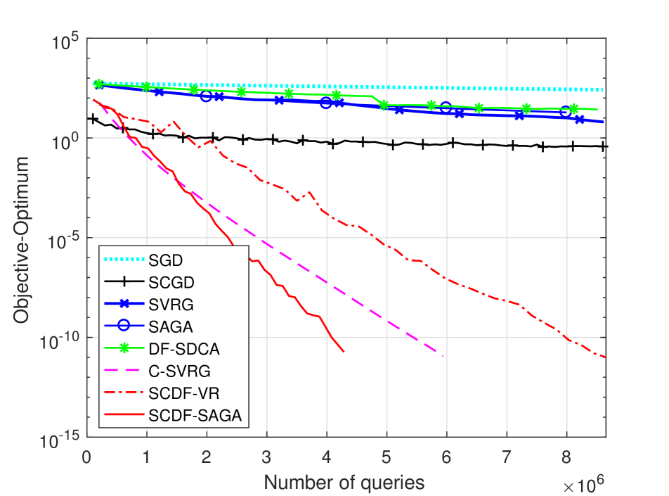
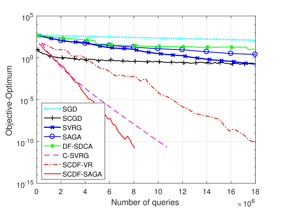
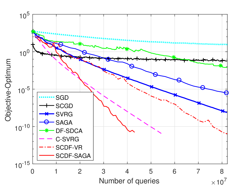
(a) $\kappa=10$

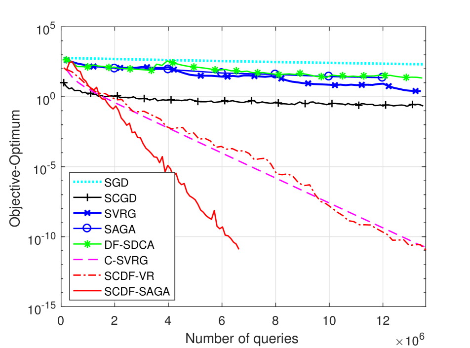
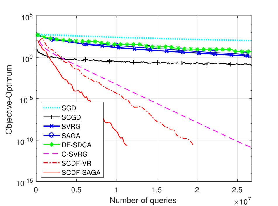
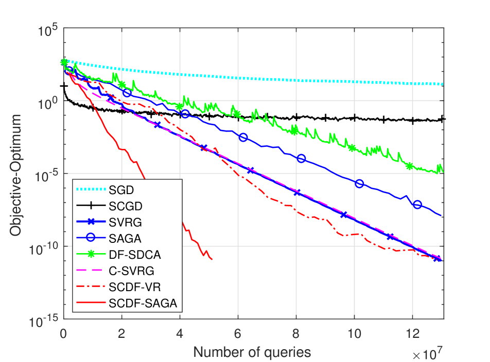
(b) $\kappa=30$

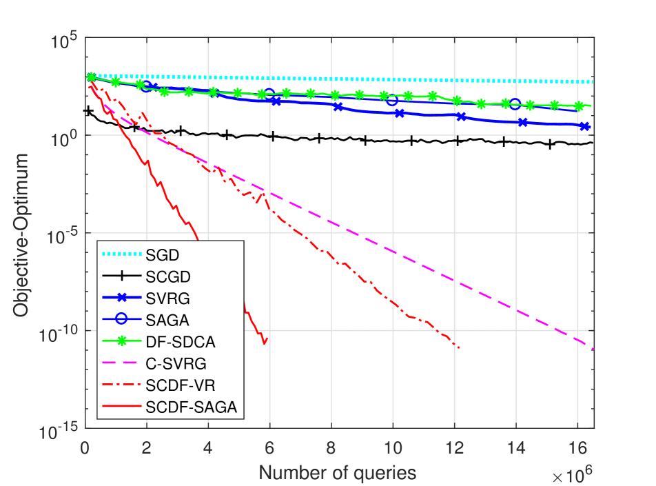
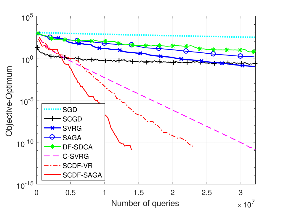
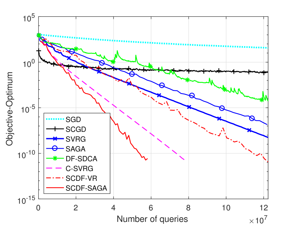
(c) $\kappa=50$

Figure 1: As the SCDF-SAGA method also has geometric convergence in expectation, the variables $x_{k}$ and $\beta_{k}$ both convergence to the optimal solution iteratively. Because they control the upper bound of the gradient, as indicated in Corollary, the variance of gradient decrease to zero.

In this section, we experiment with our two proposed algorithms and compare them with previous stochastic methods including SGD, SCGD, SVRG, SAGA, duality-free SDCA (DF-SDCA) and compositional-SVRG (C-SVRG).

To verify the effectiveness of the algorithm, we use the mean-variance optimization in portfolio management:

$$\mathop{\max}\limits_{x\in{\mathbb{R}^{d}}}\frac{1}{n}\sum\limits_{i=1}^{n}{\langle{{r_{i}},x}\rangle}-\frac{1}{n}\sum\limits_{i=1}^{n}(\langle{{r_{i}},x}\rangle-\frac{1}{n}\sum\limits_{i=1}^{n}\langle{{r_{i}},x}\rangle)^{2},$$

where $r_{i}\in\mathbb{R}^{N},i\in[n]$ is the reward vector, and $x\in\mathbb{R}^{N}$ is the invested quantity. The goal is to maximize the objective function to obtain a large investment and reduce the investment risk. The objective function can be transformed as the composition of two finite-sum functions in 1 by the following form:

$${G_{j}}(x)= {[{x,\langle{{r_{j}},x}\rangle}]^{\mathsf{T}}},\,y=\frac{1}{n}\sum\nolimits_{j=1}^{n}{{G_{j}}(x)}={[{{y_{1}},{y_{2}}}]^{\mathsf{T}}},$$

$${F_{i}}(y)= -\langle{{r_{i}},{y_{1}}}\rangle+({\langle{{r_{i}},{y_{1}}}\rangle-{y_{2}}}),j,i\in[n].$$

where $y_{1}\in\mathbb{R}^{M}$ and $y_{2}\in\mathbb{R}$. We follow the un-regularized objective method in [8], in which the term $L{\|w\|^{2}}/2$ is added or subtracted to the objective for DF-SDCA, SCDF-VR, and SCDF-SAGA, where parameter $L$ can be obtained in advance and directly from the maximal eigenvalue of the Hessian matrix. We choose $n=2000$ and $N=200$ and conduct the experiment on the numerical simulations following [9]. Reward vectors $r_{i}$, $i\in[n]$ are generated from a random Gaussian distribution under different condition numbers of the corresponding covariance matrix, denoted $\kappa$. We choose three different $\kappa=10,30$, and $50$. Furthermore, we give three different sample times for forming the mini-batch $\mathcal{A}$, $A=50,100$, and $500$. Figure 1 shows the results with different sample time $A$. From Figure 1, we can see that: 1) our proposed algorithms SCDF-SVRG and SCDF-SAGA both have linear convergence rates; and 2) SCDF-SAGA outperforms the other algorithms.

6 Conclusions

In this paper, we propose a new algorithm based on variance reduction technology and appli it to the composition of two finite-sum functions minimization problem. Unlike most previous approaches, our work applies duality-free SCDA to compositional optimization and tackles the primal and dual problems that cannot be solved directly by the primal-dual algorithm. We show linear convergence in the situation that the estimator of the inner function is biased. Furthermore, we also show a linear rate of convergence for the case in which the individual function is non-convex but the finite-sum function is strongly convex.

Appendix:

Appendix A Analysis tool

Lemma 3.

For the random variable $X$, we have

$$E[{{{\|{X-E[X]}\|}^{2}}}]{=}E[{{X^{2}}-{{\|{E[X]}\|}^{2}}}]\leq E[{{X^{2}}}].$$

Lemma 4.

For the random variable $X_{1},...,X_{r}$, we have

$$E[{{{\|{{X_{1}}+...+{X_{r}}}\|}^{2}}}]\leq r({E[{{{\|{{X_{1}}}\|}^{2}}}]+...+[{{{\|{{X_{r}}}\|}^{2}}}]}).$$

Lemma 5.

For $a$ and $b$, we have $2\langle{a,b}\rangle\leq\frac{1}{q}\|a\|^{2}+q\|b\|^{2},\forall q>0$.

Lemma 6.

Suppose Assumption 3 holds, we have

$$\frac{1}{n}\sum\limits_{i=1}^{n}{{{\|{{{(\partial G(x))}^{\mathsf{T}}}\nabla{F_{i}}(G(x))+{{(\partial G({x^{*}}))}^{\mathsf{T}}}\nabla{F_{i}}(G({x^{*}}))}\|}^{2}}}\leq 2L_{f}\left({P(x)-P({x^{*}})-\frac{\lambda}{2}{{\|{x-{x^{*}}}\|}^{2}}}\right).$$

Proof.

Based on $L_{F}$-smoothness and convexity of $F_{i}$ in (8), we have

$$\frac{1}{n}\sum\limits_{i=1}^{n}{{{\|{{(\partial G(x))^{\mathsf{T}}}\nabla{F_{i}}(G(x))-{(\partial G({x^{*}}))^{\mathsf{T}}}\nabla{F_{i}}(G({x^{*}}))}\|}^{2}}}$$

$$\leq \frac{1}{n}\sum\limits_{i=1}^{n}{2L_{f}({{F_{i}}(G(x))-\nabla{F_{i}}(G({x^{*}}))-\langle{{(\partial G({x^{*}}))^{\mathsf{T}}}\nabla{F_{i}}(G({x^{*}})),x-{x^{*}}}\rangle})}$$

$$= 2L_{f}({F(x)-F({x^{*}})-\langle{F({x^{*}}),x-{x^{*}}}\rangle})$$

$$= 2L_{f}({F(x)+R(x)-F({x^{*}})-R({x^{*}})-R(x)+R({x^{*}})-\langle{\nabla P({x^{*}})+\nabla R({x^{*}})-\nabla R({x^{*}}),x-{x^{*}}}\rangle})$$

$$= 2L_{f}({P(x)-P({x^{*}})})+\underbrace{2L({-R(x)+R({x^{*}})-\langle{-\nabla R({x^{*}}),x-{x^{*}}}\rangle})}_{(App1)}$$

$$= 2L_{f}({P(x)-P({x^{*}})-\frac{\lambda}{2}{{\|{x-{x^{*}}}\|}^{2}}}),$$

where (App1) is based on the smoothness of $R(x)$, that is $R(x)=\frac{1}{2}\lambda{\|x\|^{2}}$, the smooth constant is $\lambda$, then we have

$$-R(x)+R({x^{*}})+\langle{\nabla R({x^{*}}),x-{x^{*}}}\rangle\leq -\frac{1}{{2L_{f}}}{\|{\nabla R({x^{*}})-R(x)}\|^{2}}$$

$$\leq -\frac{\lambda}{2}{\|{x-{x^{*}}}\|^{2}}.$$

∎

Appendix B Proof of SCDF-SVRG

Proof of Lemma 1

Proof.

$$E[{\|{{(\partial{{\hat{G}}_{k}})^{\mathsf{T}}}\nabla{F_{i}}({{\hat{G}}_{k}})-{(\partial{{\hat{G}}_{k}})^{\mathsf{T}}}\nabla{F_{i}}(G({x_{k}}))}\|^{2}}]$$

$$\leq B_{G}^{2}E[{\|{\nabla{F_{i}}({{\hat{G}}_{k}})-\nabla{F_{i}}(G({x_{k}}))}\|^{2}}]$$

$$\leq B_{G}^{2}L_{F}^{2}E[{\|{{{\hat{G}}_{k}}-G({x_{k}})}\|^{2}}]$$

$$\leq B_{G}^{4}L_{F}^{2}\frac{1}{A}E[{\|{{x_{k}}-{{\tilde{x}}_{s}}}\|^{2}}]$$

$$\leq B_{G}^{4}L_{F}^{2}\frac{1}{A}E[{\|{{x_{k}}-{{x}^{*}}}\|^{2}}]+B_{G}^{4}L_{F}^{2}\frac{1}{A}E[{\|{{{\tilde{x}}_{s}}}-x^{*}\|^{2}}],$$

where the first and the second inequalities is based on the bounded Jacobian of $G$ and Lipschitz continuous gradient of $F$. The last inequality follows from Lemma 7. ∎

Proof of Theorem 1

Proof.

Based on Lemma 14, we have

$${C_{k}}-{C_{k-1}}\leq-\eta\lambda{C_{k-1}}+{d_{2}}E[{\|{{{\tilde{x}}_{s}}-{x^{*}}}\|^{2}}],$$

where ${d_{2}}=2\left({a\eta qB_{G}^{4}L_{F}^{2}\frac{1}{A}+b\lambda\eta\left({4B_{F}^{2}L_{G}^{2}\frac{1}{A}+4B_{G}^{4}L_{F}^{2}}\right)}\right)+b\lambda\eta\left({4B_{F}^{2}L_{G}^{2}+4B_{G}^{4}L_{F}^{2}}\right)$. Summing from k=0 to K, we obtain

$${C_{K}}+\eta\lambda\sum\limits_{k=1}^{K-1}{{C_{k}}}\leq{C_{0}}+K{d_{2}}E[{\|{{{\tilde{x}}_{s}}-{x^{*}}}\|^{2}}].$$

Since ${C_{0}}={{\tilde{C}}_{s}}$ and ${{\tilde{C}}_{s+1}}=\frac{1}{K}\sum\nolimits_{k=1}^{K}{{C_{k}}}$, and $\eta\lambda\leq 1$, we have

$$\eta\lambda K{{\tilde{C}}_{s+1}}=\eta\lambda\frac{1}{K}\sum\limits_{k=1}^{K}{{C_{k}}}\leq{C_{0}}+K{d_{2}}E[{\|{{{\tilde{x}}_{s}}-{x^{*}}}\|^{2}}].$$

The definition of ${{\tilde{C}}_{s}}$ implies that $aE[{\|{{{\tilde{x}}_{s}}-{x^{*}}}\|^{2}}]\leq{{\tilde{C}}_{s}}$. Therefore we have

$$\eta\lambda K{{\tilde{C}}_{s+1}}\leq{C_{0}}+\frac{{K{d_{2}}}}{a}{{\tilde{C}}_{s}}.$$

Dividing both sides of the inequality by $\eta\lambda K$, we can obtain the linear convergence,

$${{\tilde{C}}_{s+1}}\leq\left({\frac{1}{{\eta\lambda K}}+\frac{{{d_{2}}}}{{a\eta\lambda}}}\right){{\tilde{C}}_{s}}\leq{\left({\frac{1}{{\eta\lambda K}}+\frac{{{d_{2}}}}{{a\eta\lambda}}}\right)^{s}}{{\tilde{C}}_{0}}.$$

∎

Proof of Theorem 2

Proof.

The proof process is similar to Theorem 1, but based on different inner estimation bound from Lemma 15 ∎

Proof of Corollary 1

Proof.

Based on Lemma 4, we have

$$E[{\|{{({\partial{{\hat{G}}_{k}}})^{\mathsf{T}}}\nabla{F_{i}}({{{\hat{G}}_{k}}})+\beta_{i}^{k}}\|^{2}}]$$

$$\leq 2E[{\|{{({\partial{{\hat{G}}_{k}}})^{\mathsf{T}}}\nabla{F_{i}}({{{\hat{G}}_{k}}})+\beta_{i}^{*}}\|^{2}}]+2E[{\|{\beta_{i}^{k}-\beta_{i}^{*}}\|^{2}}]$$

$$\leq \left({4B_{F}^{2}L_{G}^{2}\frac{1}{A}+4B_{G}^{4}L_{F}^{2}\frac{1}{A}}\right)E[{\|{{x_{k}}-{{\tilde{x}}_{s}}}\|^{2}}]+({4B_{F}^{2}L_{G}^{2}+4B_{G}^{4}L_{F}^{2}})E[{\|{{{\tilde{x}}_{s}}-{x^{*}}}\|^{2}}]+E[{\|{\beta_{i}^{k}-\beta_{i}^{*}}\|^{2}}],$$

where the first inequality follows from Lemma 12. ∎

Appendix C Proof of SCDF-SAGA

Proof of Lemma 2

Proof.

Through subtracting and adding ${{(\partial G({x_{k}}))^{\mathsf{T}}}\nabla{F_{i}}({{\hat{G}}_{k}})}$, we have

$$E[{\|{{(\partial{{\hat{G}}_{k}})^{\mathsf{T}}}\nabla{F_{i}}({{\hat{G}}_{k}})-{(\partial G({x_{k}}))^{\mathsf{T}}}\nabla{F_{i}}({G_{k}}({x_{k}}))}\|^{2}}]$$

$$= E[{\|{{(\partial{{\hat{G}}_{k}})^{\mathsf{T}}}\nabla{F_{i}}({{\hat{G}}_{k}})-{(\partial G({x_{k}}))^{\mathsf{T}}}\nabla{F_{i}}({{\hat{G}}_{k}})+{(\partial G({x_{k}}))^{\mathsf{T}}}\nabla{F_{i}}({{\hat{G}}_{k}})-{(\partial G({x_{k}}))^{\mathsf{T}}}\nabla{F_{i}}({G_{k}}({x_{k}}))}\|^{2}}]$$

$$\leq 2E[{\|{{(\partial{{\hat{G}}_{k}})^{\mathsf{T}}}\nabla{F_{i}}({{\hat{G}}_{k}})-(\partial G{({x_{k}})^{\mathsf{T}}}\nabla{F_{i}}({{\hat{G}}_{k}})}\|^{2}}]$$

$$+2E[{\|{{(\partial G({x_{k}}))^{\mathsf{T}}}\nabla{F_{i}}({{\hat{G}}_{k}})-{(\partial G({x_{k}}))^{\mathsf{T}}}\nabla{F_{i}}({G_{k}}({x_{k}}))}\|^{2}}]$$

$$\leq 2B_{F}^{2}E[{\|{\partial{{\hat{G}}_{k}}-\partial G({x_{k}})}\|^{2}}]+2B_{G}^{2}E[{\|{\nabla{F_{i}}({{\hat{G}}_{k}})-\nabla{F_{i}}(\partial G({x_{k}}))}\|^{2}}]$$

$$\leq 2B_{F}^{2}E[{\|{\partial{{\hat{G}}_{k}}-\partial G({x_{k}})}\|^{2}}]+2B_{G}^{2}L_{F}^{2}E[{\|{{{\hat{G}}_{k}}-G({x_{k}})}\|^{2}}]$$

$$\leq 2B_{F}^{2}L_{G}^{2}\frac{1}{{{A^{2}}}}\sum\limits_{1\leq j\leq A}{E[{\|{{x_{k}}-\phi_{{{\cal A}_{k}}[j]}^{k}}\|^{2}}]}+2B_{G}^{2}L_{F}^{2}B_{G}^{2}\frac{1}{{{A^{2}}}}\sum\limits_{1\leq j\leq A}{E[{\|{{x_{k}}-\phi_{{{\cal A}_{k}}[j]}^{k}}\|^{2}}]}$$

$$= \left({2B_{F}^{2}L_{G}^{2}+2B_{G}^{4}L_{F}^{2}}\right)\frac{1}{{{A^{2}}}}\sum\limits_{1\leq j\leq A}{E[{\|{{x_{k}}-\phi_{{{\cal A}_{k}}[j]}^{k}}\|^{2}}]}$$

where the first inequality follows from Lemma 4, The second and third are based on the bounded gradient of $F_{i}$ in (3), the bounded Jacobian of $G$ in (5) and Lipschitz continuous gradient of $F$ in (4), The last inequality follows from the Lemma 21 and Lemma 22. ∎

Proof of Theorem 3

Proof.

Based on Lemma 26, Lemma 28 and Lemma 30, let ${D_{k}}=aE[{{A_{k}}}]+bE[{{B_{k}}}]+cnE[{{C_{k}}}]$, we have

$${D_{k+1}}-{D_{k}}$$

$$= a({E[{{A_{k+1}}}]-E[{{A_{k}}}]})+b({E[{{B_{k+1}}}]-E[{{B_{k}}}]})+c({nE[{{C_{k+1}}}]-nE[{{C_{k}}}]})$$

$$\leq -a\eta\lambda E\left[{{A_{k}}}\right]-b\lambda\eta E\left[{{B_{k}}}\right]-c\lambda\eta nE\left[{{C_{k}}}\right]$$

$$+\underbrace{\left({8a\lambda\eta{R_{x}}\left({B_{F}^{2}L_{G}^{2}+B_{G}^{4}L_{F}^{2}}\right)\frac{1}{A}-a\eta\lambda+2\lambda\eta b\left({B_{F}^{2}L_{G}^{2}\frac{1}{A}+B_{G}^{4}L_{F}^{2}}\right)+cA}\right)}_{{E_{1}}}E\left[{{A_{k}}}\right]$$

$$+\underbrace{\left({8a\lambda\eta{R_{x}}\left({B_{F}^{2}L_{G}^{2}+B_{G}^{4}L_{F}^{2}}\right)\frac{1}{A}+2b\lambda\eta B_{F}^{2}L_{G}^{2}\frac{1}{A}-cA+c\lambda\eta n}\right)}_{{E_{2}}}E\left[{{C_{k}}}\right]$$

$$+\underbrace{({a{\eta^{2}}-(1-\lambda n\eta)b\lambda\eta})}_{{E_{3}}}{\|{{(\partial{{\hat{G}}_{k}})^{\mathsf{T}}}\nabla{F_{i}}({{\hat{G}}_{k}})+\beta_{i}^{k}}\|^{2}},$$

by setting the last terms $E_{1}$, $E_{2}$ and $E_{3}$ negative. Thus, we can obtain

$${D_{k+1}}-{D_{k}}\leq-\lambda\eta{D_{k}},$$

In order to simply the analysis, we define ${Y_{1}}={R_{x}}\left({B_{F}^{2}L_{G}^{2}+B_{G}^{4}L_{F}^{2}}\right)\frac{1}{A},{Y_{2}}=B_{F}^{2}L_{G}^{2}\frac{1}{A}+B_{G}^{4}L_{F}^{2},{Y_{3}}=B_{F}^{2}L_{G}^{2}\frac{1}{A}$. Both $E_{1}$ and $E_{2}$ are negative, we get

$$\frac{a}{b}\geq\frac{{2{Y_{2}}+\frac{A}{{A-\lambda\eta n}}2{Y_{3}}}}{{1-8\left({1+\frac{A}{{A-\lambda\eta n}}}\right){Y_{1}}}}.$$ (17)

To keep the bound positive, that is $1-8{Y_{1}}-8\frac{A}{{A-\lambda\eta}}Y\geq 0$, the sample times $A$ satisfy,

$$A\geq\frac{{\left({\lambda\eta n+2{R_{x}}\left({B_{F}^{2}L_{G}^{2}+B_{G}^{4}L_{F}^{2}}\right)}\right)+\sqrt{{\lambda^{2}}{\eta^{2}}{n^{2}}+4{{\left({{R_{x}}\left({B_{F}^{2}L_{G}^{2}+B_{G}^{4}L_{F}^{2}}\right)}\right)}^{2}}}}}{2}.$$

Based on above condition in (17) and $E_{3}\leq 0$, we have

$$\frac{{2{Y_{2}}+\frac{A}{{A-\lambda\eta n}}2{Y_{3}}}}{{1-8\left({1+\frac{A}{{A-\lambda\eta n}}}\right){Y_{1}}}}\leq\frac{{(1-\lambda n\eta)\lambda}}{\eta},$$

Thus, we get

$$\eta\leq\frac{\lambda}{{2{Y_{2}}+\frac{A}{{A-\lambda\eta n}}2{Y_{3}}+{\lambda^{2}}n\left({1-8\left({1+\frac{A}{{A-\lambda\eta n}}}\right){Y_{1}}}\right)}}.$$

Finally, we can obtain the convergence form,

$$aE\left[{{A_{k+1}}}\right]+bE\left[{{B_{k+1}}}\right]+cnE\left[{{C_{k+1}}}\right]\leq{\left({1-\eta\lambda}\right)^{k}}\left({aE\left[{{A_{1}}}\right]+bE\left[{{B_{1}}}\right]+cnE\left[{{C_{1}}}\right]}\right),$$

∎

Proof of Theorem 4

Proof.

Based on Lemma 27, Lemma 29 and Lemma 30, let ${D_{k}}=aE[{{A_{k}}}]+bE[{{B_{k}}}]+cnE[{{C_{k}}}]$, we have

$${D_{k+1}}-{D_{k}}$$

$$= a\left({E\left[{{A_{k+1}}}\right]-E\left[{{A_{k}}}\right]}\right)+b\left({E\left[{{B_{k+1}}}\right]-E\left[{{B_{k}}}\right]}\right)+c\left({nE\left[{{C_{k+1}}}\right]-nE\left[{{C_{k}}}\right]}\right)$$

$$\leq -a\eta\lambda E[{{A_{k}}}]-b\lambda\eta E[{{B_{k}}}]-c\lambda\eta nE[{{C_{k}}}]$$

$$+\underbrace{\left({8a\eta\lambda{R_{x}}({B_{F}^{2}L_{G}^{2}+B_{G}^{4}L_{F}^{2}})\frac{1}{A}-a\eta d\lambda+4b\lambda\eta({B_{F}^{2}L_{G}^{2}+B_{G}^{4}L_{F}^{2}})\frac{1}{A}-2b{L_{f}}{\lambda^{2}}\eta+cA}\right)}_{{E_{1}}}E[{{A_{k}}}]$$

$$+\underbrace{\left({8a\eta\lambda{R_{x}}({B_{F}^{2}L_{G}^{2}+B_{G}^{4}L_{F}^{2}})\frac{1}{A}+4b\lambda\eta({B_{F}^{2}L_{G}^{2}+B_{G}^{4}L_{F}^{2}})\frac{1}{A}-cA+c\lambda\eta n}\right)}_{{E_{2}}}E[{{C_{k}}}]$$

$$+\underbrace{({a{\eta^{2}}-(1-\lambda n\eta)b\lambda\eta})}_{{E_{3}}}{\|{{(\partial{{\hat{G}}_{k}})^{\mathsf{T}}}\nabla{F_{i}}({{\hat{G}}_{k}})+\beta_{i}^{k}}\|^{2}}+\underbrace{({-2a({1-d})\eta+4b{L_{f}}\lambda\eta})}_{{E_{4}}}(P({x_{k}})-P({x^{*}})).$$

by setting the last four terms negative, we can obtain

$${D_{k+1}}-{D_{k}}\leq-\lambda\eta{D_{k}}.$$

Define $Y=\left({B_{F}^{2}L_{G}^{2}+B_{G}^{4}L_{F}^{2}}\right)\frac{1}{A}$ for simply analysis. Based on $E_{1}$ and $E_{2}$ that should be negative, we have

$$\frac{a}{b}\geq\frac{{4Y+\frac{A}{{A-\lambda\eta n}}4Y-2{L_{f}}\lambda}}{{d-8\left({1+\frac{A}{{A-\lambda\eta n}}}\right){R_{x}}Y}},$$ (18)

In order to keep the bound positive, the sample times $A$ should satisfy

$$A\geq({2+\sqrt{2}})\left({\lambda\eta n+\frac{{16{R_{x}}({B_{F}^{2}L_{G}^{2}+B_{G}^{4}L_{F}^{2}})}}{d}}\right).$$

Based on $E_{3}$ and $E_{4}$ that should be negative, we have

$$\frac{{2{L_{f}}\lambda}}{{\left({1-d}\right)}}\leq\frac{a}{b}\leq\frac{{(1-\lambda n\eta)\lambda}}{\eta}.$$

Thus, we can get the upper bound of the step

$$\eta\leq\frac{1}{{\left({\frac{{2{L_{f}}\lambda}}{{\left({1-d}\right)}}+\lambda n}\right)}},$$

where the parameter $d$ satisfy,

$$d\leq\frac{{\left({4Y+\frac{A}{{A-\lambda\eta n}}4Y-2{L_{f}}\lambda}\right)+8\left({1+\frac{A}{{A-\lambda\eta n}}}\right){R_{x}}Y2{L_{F}}\lambda}}{{4Y+\frac{A}{{A-\lambda\eta n}}4Y}}.$$

Thus we can obtain the convergence form

$$aE\left[{{A_{k+1}}}\right]+bE\left[{{B_{k+1}}}\right]+cnE\left[{{C_{k+1}}}\right]\leq{\left({1-\eta\lambda}\right)^{k}}\left({aE\left[{{A_{1}}}\right]+bE\left[{{B_{1}}}\right]+cnE\left[{{C_{1}}}\right]}\right),$$

∎

Note that as the variable $x_{k}$ and $\beta^{k}$ go to the optimal solution, we can see that the variance of gradient in the update iteration is also approximating to zero. The following Corollary shows the bound of the estimated gradient variance

Proof of Corollary 2

Proof.

Based on the update of $x_{k}$, we have

$$\frac{1}{{{\eta^{2}}}}E[{{{\|{({{x_{k+1}}-{x_{k}}})}\|}^{2}}}]$$

$$= E[{\|{{({\partial{{\hat{G}}_{k}}})^{\mathsf{T}}}\nabla{F_{i}}({{{\hat{G}}_{k}}})+\beta_{i}^{k}}\|^{2}}]$$

$$\leq 2E[{\|{{({\partial{{\hat{G}}_{k}}})^{\mathsf{T}}}\nabla{F_{i}}({{{\hat{G}}_{k}}})+\beta_{i}^{*}}\|^{2}}]+2E[\|\beta^{k}-\beta^{*}\|^{2}]$$

$$\leq 4\left({B_{F}^{2}L_{G}^{2}\frac{1}{A}+B_{G}^{4}L_{F}^{2}}\right)E[{\|{{x_{k}}-{x^{*}}}\|^{2}}]+4B_{F}^{2}L_{G}^{2}\frac{1}{{{A^{2}}}}\sum\limits_{1\leq j\leq A}{E[{\|{\phi_{{\mathcal{A}_{k}}[j]}^{k}-{x^{*}}}\|^{2}}]}+2E[\|\beta^{k}-\beta^{*}\|^{2}],$$

where the first and second inequalities follows from Lemma 24 and Lemma 4. ∎

Appendix D Convergence Bound Analysis for SDFC-SVRG

D.1 Bounding the estimation of inner function $G$

Lemma 7.

Assumption 2 holds, in algorithm 2, for the intermediated iteration of $x_{k}$ and $\tilde{x}_{s}$, and $\hat{G}_{k}$ defined in (11), the variance of stochastic gradient is ,

$$E[{\|{{{\hat{G}}_{k}}-G({{x_{k}}})}\|^{2}}]\leq B_{G}^{2}\frac{1}{A}E[{\|{{x_{k}}-{{\tilde{x}}_{s}}}\|^{2}}],$$

where $B_{G}$ is the parameter in (5).

Proof.

Based on the bounded Jacobian of $G_{j}$ and Lipschitz continuous gradient of $F_{i}$, $j\in[m]$, $i\in[n]$, we have

$$E[{\|{{{\hat{G}}_{k}}-G({{x_{k}}})}\|^{2}}]$$

$$= E[{\|{\frac{1}{A}\sum\limits_{1\leq j\leq A}{({{G_{{{\cal A}_{k}}[j]}}({{x_{k}}})-{G_{{{\cal A}_{k}}[j]}}({{{\tilde{x}}_{s}}})})}+G({{{\tilde{x}}_{s}}})-G({{x_{k}}})}\|^{2}}]$$

$$\leq \frac{1}{{{A^{2}}}}\sum\limits_{1\leq j\leq A}{{E[{\|{{G_{{{\cal A}_{k}}[j]}}({{x_{k}}})-{G_{{{\cal A}_{k}}[j]}}({{{\tilde{x}}_{s}}})-({G({{x_{k}}})-G({{{\tilde{x}}_{s}}})})}\|^{2}}]}}$$

$$\leq \frac{1}{{{A^{2}}}}\sum\limits_{1\leq j\leq A}{{E[{\|{{G_{{{\cal A}_{k}}[j]}}({{x_{k}}})-{G_{{{\cal A}_{k}}[j]}}({{{\tilde{x}}_{s}}})}\|^{2}}]}}$$

$$\leq B_{G}^{2}\frac{1}{A}E[{\|{{x_{k}}-{{\tilde{x}}_{s}}}\|^{2}}],$$

where the first and second inequalities follow from Lemma (3) and (4), and the third inequality is based on the bounded Jacobian of $G$ in (5). ∎

Lemma 8.

Assumption 2 holds, in algorithm 2, for the intermediated iteration of $x_{k}$ and $\tilde{x}_{s}$, and $\partial\hat{G}_{k}$ defined in (12), the variance of stochastic gradient is ,

$$E[{\|{\partial{{\hat{G}}_{k}}-\partial G({{x_{k}}})}\|^{2}}]\leq L_{G}^{2}\frac{1}{A}E[{\|{{x_{k}}-{{\tilde{x}}_{s}}}\|^{2}}],$$

where $B_{G}$ is the parameter in (5).

Proof.

Based on the bounded Jacobian of $G_{j}$ and Lipschitz continuous gradient of $F_{i}$, $j\in[m]$, $i\in[n]$, we have

$$E[{\|{\partial{{\hat{G}}_{k}}-\partial G({{x_{k}}})}\|^{2}}]$$

$$= E[{\|{\frac{1}{A}\sum\limits_{1\leq j\leq A}{({\partial{G_{{{\cal A}_{k}}[j]}}({{x_{k}}})-\partial{G_{{{\cal A}_{k}}[j]}}({{{\tilde{x}}_{s}}})})}+\partial G({{{\tilde{x}}_{s}}})-\partial G({{x_{k}}})}\|^{2}}]$$

$$\leq \frac{1}{{{A^{2}}}}\sum\limits_{1\leq j\leq A}{{E[{\|{\partial{G_{{{\cal A}_{k}}[j]}}({{x_{k}}})-\partial{G_{{{\cal A}_{k}}[j]}}({{{\tilde{x}}_{s}}})-({\partial G({{x_{k}}})-\partial G({{{\tilde{x}}_{s}}})})}\|^{2}}]}}$$

$$\leq \frac{1}{{{A^{2}}}}\sum\limits_{1\leq j\leq A}{{E[{\|{\partial{G_{{{\cal A}_{k}}[j]}}({{x_{k}}})-{\partial G_{{{\cal A}_{k}}[j]}}({{{\tilde{x}}_{s}}})}\|^{2}}]}}$$

$$\leq L_{G}^{2}\frac{1}{A}E[{\|{{x_{k}}-{{\tilde{x}}_{s}}}\|^{2}}],$$

where the first and second inequalities follow from Lemma (3) and (4), and the third inequality is based on the bounded Jacobian of $G$ in (5). ∎

Lemma 9.

Assumption 2 holds, in algorithm 2, for the intermediated iteration of $x_{k}$ and $\tilde{x}_{s}$ and $\hat{G}_{k}$ defined in (11), the bound satisfies,

$$E[{\|{{{\hat{G}}_{k}}-G({{x^{*}}})}\|^{2}}]\leq{2B_{G}^{2}\frac{1}{A}E[{\|{{x_{k}}-{{\tilde{x}}_{s}}}\|^{2}}]+2B_{G}^{2}E[{\|{{{\tilde{x}}_{s}}-{x^{*}}}\|^{2}}]},$$

where $B_{G}$ is the parameter in (5).

Proof.

From the definition of $\hat{G}_{k}$ in (11),we have

$$E[{\|{{{\hat{G}}_{k}}-G({{x^{*}}})}\|^{2}}]$$

$$= E[{\|{\frac{1}{A}\sum\limits_{1\leq j\leq A}{({{G_{{{\cal A}_{k}}[j]}}({{x_{k}}})-{G_{{{\cal A}_{k}}[j]}}({{{\tilde{x}}_{s}}})})}+G({{{\tilde{x}}_{s}}})-G({{x^{*}}})}\|^{2}}]$$

$$\leq {2E[{\|{\frac{1}{A}\sum\limits_{1\leq j\leq A}{({{G_{{{\cal A}_{k}}[j]}}({{x_{k}}})-{G_{{{\cal A}_{k}}[j]}}({{{\tilde{x}}_{s}}})})}}\|^{2}}]+2E[{\|{G({{{\tilde{x}}_{s}}})-G({{x^{*}}})}\|^{2}}]}$$

$$\leq 2\frac{1}{{{A^{2}}}}\sum\limits_{1\leq j\leq A}{E{{\|{{G_{{A_{k}}[j]}}({x_{k}})-{G_{{A_{k}}[j]}}({{\tilde{x}}_{s}})}\|}^{2}}}+2E[{\|{G({{{\tilde{x}}_{s}}})-G({{x^{*}}})}\|^{2}}]$$

$$\leq {2B_{G}^{2}\frac{1}{A}E[{\|{{x_{k}}-{{\tilde{x}}_{s}}}\|^{2}}]+2B_{G}^{2}E[{\|{{{\tilde{x}}_{s}}-{x^{*}}}\|^{2}}]},$$

where the first and the second inequalities follow from Lemma 4, and the third inequality is based on the bounded Jacobian of $G$ in (5). ∎

Lemma 10.

Assumption 2 holds, in algorithm 2, for the intermediated iteration of $x_{k}$ and $\tilde{x}_{s}$ and $\partial\hat{G}_{k}$ defined in (12), the bound satisfies,

$$E[{\|{\partial{{\hat{G}}_{k}}-\partial G({{x^{*}}})}\|^{2}}]\leq{2L_{G}^{2}\frac{1}{A}E[{\|{{x_{k}}-{{\tilde{x}}_{s}}}\|^{2}}]+2L_{G}^{2}E[{\|{{{\tilde{x}}_{s}}-{x^{*}}}\|^{2}}]},$$

where $L_{G}$ is the parameter in (6).

Proof.

$$E[{\|{\partial{{\hat{G}}_{k}}-\partial G({{x^{*}}})}\|^{2}}]$$

$$= E[{\|{\frac{1}{A}\sum\limits_{1\leq j\leq A}{({\partial{G_{{{\cal A}_{k}}[j]}}({{x_{k}}})-\partial{G_{{{\cal A}_{k}}[j]}}({{{\tilde{x}}_{s}}})})}+\partial G({{{\tilde{x}}_{s}}})-\partial G({{x^{*}}})}\|^{2}}]$$

$$\leq {2E[{\|{\frac{1}{A}\sum\limits_{1\leq j\leq A}{({\partial{G_{{{\cal A}_{k}}[j]}}({{x_{k}}})-\partial{G_{{{\cal A}_{k}}[j]}}({{{\tilde{x}}_{s}}})})}}\|^{2}}]+2E[{\|{\partial G({{{\tilde{x}}_{s}}})-\partial G({{x^{*}}})}\|^{2}}]}$$

$$\leq 2\frac{1}{{{A^{2}}}}\sum\limits_{1\leq j\leq A}{E{{\|{{\partial G_{{A_{k}}[j]}}({x_{k}})-{\partial G_{{A_{k}}[j]}}({{\tilde{x}}_{s}})}\|}^{2}}}+2E[{\|{\partial G({{{\tilde{x}}_{s}}})-\partial G({{x^{*}}})}\|^{2}}]$$

$$\leq {2L_{G}^{2}\frac{1}{A}E[{\|{{x_{k}}-{{\tilde{x}}_{s}}}\|^{2}}]+2L_{G}^{2}E[{\|{{{\tilde{x}}_{s}}-{x^{*}}}\|^{2}}]},$$

where the first and the second inequalities follow from Lemma 4 and the Lipschitz continuous gradient of $G$ in (6). ∎

D.2 Bounding the estimation of function $F$

Lemma 11.

Suppose Assumption 2 and 3 holds, in algorithm 2, for the intermediated iteration at $x_{k}$ and $\tilde{x}_{s}$, and $\hat{G}_{k}$ and $\partial\hat{G}_{k}$ defined in (12) and (11), we have

$$E[\|(\partial{{\hat{G}}_{k}})^{\mathsf{T}}\nabla{F_{i}}({{\hat{G}}_{k}})-(\partial G({x_{k}}))^{\mathsf{T}}\nabla{F_{i}}(G(x_{k}))\|^{2}]$$

$$\leq 2\left(B_{F}^{2}L_{G}^{2}+B_{G}^{4}L_{F}^{2}\right)\frac{1}{A}E[{\|{{x_{k}}-x^{*}}\|^{2}}]+2\left(B_{F}^{2}L_{G}^{2}+B_{G}^{4}L_{F}^{2}\right)\frac{1}{A}E[{\|{{{\tilde{x}}_{s}}-x^{*}}\|^{2}}]$$

where $L_{F}$ and $B_{G}$ are the parameters in (4) and (5).

Proof.

Through subtracting and adding $(\partial G({x_{k}}))^{\mathsf{T}}\nabla{F_{i}}({{\hat{G}}_{k}})$

$$E[\|(\partial{{\hat{G}}_{k}})^{\mathsf{T}}\nabla{F_{i}}({{\hat{G}}_{k}})-(\partial G({x_{k}}))^{\mathsf{T}}\nabla{F_{i}}(G(x_{k}))\|^{2}]$$

$$\leq E[\|(\partial{{\hat{G}}_{k}})^{\mathsf{T}}\nabla{F_{i}}({{\hat{G}}_{k}})-(\partial G({x_{k}}))^{\mathsf{T}}\nabla{F_{i}}({{\hat{G}}_{k}})+(\partial G({x_{k}}))^{\mathsf{T}}\nabla{F_{i}}({{\hat{G}}_{k}})-(\partial G({x_{k}}))^{\mathsf{T}}\nabla{F_{i}}(G(x_{k}))\|^{2}]$$

$$\leq 2B_{F}^{2}E[\|\partial{{\hat{G}}_{k}}-\partial G({x_{k}})\|^{2}]+2B_{G}^{2}E[\|\nabla{F_{i}}({{\hat{G}}_{k}})-\nabla{F_{i}}(G(x_{k}))\|^{2}]$$

$$\leq 2B_{F}^{2}E[\|\partial{{\hat{G}}_{k}}-\partial G({x_{k}})\|^{2}]+2B_{G}^{2}L_{F}^{2}E[\|{{\hat{G}}_{k}}-G(x_{k})\|^{2}]$$

$$\leq 2B_{F}^{2}L_{G}^{2}\frac{1}{A}E[{\|{{x_{k}}-{{\tilde{x}}_{s}}}\|^{2}}]+2B_{G}^{2}L_{F}^{2}B_{G}^{2}\frac{1}{A}E[{\|{{x_{k}}-{{\tilde{x}}_{s}}}\|^{2}}]$$

$$\leq \left(2B_{F}^{2}L_{G}^{2}\frac{1}{A}+2B_{G}^{2}L_{F}^{2}B_{G}^{2}\frac{1}{A}\right)E[{\|{{x_{k}}-x^{*}}\|^{2}}]+\left(2B_{F}^{2}L_{G}^{2}\frac{1}{A}+2B_{G}^{2}L_{F}^{2}B_{G}^{2}\frac{1}{A}\right)E[{\|{{{\tilde{x}}_{s}}-x^{*}}\|^{2}}]$$

where the first and the second inequalities is based on the bounded Jacobian of $G$ and Lipschitz continuous gradient of $F$. The last inequality follows from Lemma 7. ∎

Lemma 12.

Suppose Assumption 2 holds, in algorithm 2, for the intermediated iteration at $\beta_{k}$, $\hat{G}_{k}$ and $\partial\hat{G}_{k}$ defined in (12) and (11), we have,

$$E[{\|{{({\partial{{\hat{G}}_{k}}})^{\mathsf{T}}}\nabla{F_{i}}({{{\hat{G}}_{k}}})+\beta_{i}^{*}}\|^{2}}]\leq 4({B_{F}^{2}L_{G}^{2}+B_{G}^{4}L_{F}^{2}})\frac{1}{A}E[\|{{x_{k}}-x^{*}\|^{2}}]+4({B_{F}^{2}L_{G}^{2}+B_{G}^{4}L_{F}^{2}})\left(1+\frac{1}{A}\right)E[\|{\tilde{x}}_{s}-x^{*}\|^{2}],$$

where $L_{G}$, $L_{F}$, $B_{G}$ and $B_{F}$ are the parameters in (3) - (7).

Proof.

Based on the relationship between $\beta_{i}^{*}$ and ${({\partial G({{x^{*}}})})^{\mathsf{T}}}\nabla{F_{i}}({G({{x^{*}}})})$, we have

$$E[{\|{{(\partial{{\hat{G}}_{k}})^{\mathsf{T}}}\nabla{F_{i}}({{\hat{G}}_{k}})+\beta_{i}^{*}}\|^{2}}]=E[{\|{{(\partial{{\hat{G}}_{k}})^{\mathsf{T}}}\nabla{F_{i}}({{\hat{G}}_{k}})-{({\partial G({{x^{*}}})})^{\mathsf{T}}}\nabla{F_{i}}({G({{x^{*}}})})}\|^{2}}].$$

Through subtracting and adding ${{({\partial G({{x_{k}}})})^{\mathsf{T}}}\nabla{F_{i}}({{{G}_{k}}})}$, we obtain

$$E[{\|{{(\partial{{\hat{G}}_{k}})^{\mathsf{T}}}\nabla{F_{i}}({{\hat{G}}_{k}})-{({\partial G({{x^{*}}})})^{\mathsf{T}}}\nabla{F_{i}}({G({{x^{*}}})})}\|^{2}}]$$

$$= E[{\|{{(\partial{{\hat{G}}_{k}})^{\mathsf{T}}}\nabla{F_{i}}({{\hat{G}}_{k}})-{({\partial G({{x^{*}}})})^{\mathsf{T}}}\nabla{F_{i}}({{\hat{G}}_{k}})+{{({\partial G({{x^{*}}})})}^{\mathsf{T}}}\nabla{F_{i}}({{\hat{G}}_{k}})-{{({\partial G({{x^{*}}})})}^{\mathsf{T}}}\nabla{F_{i}}({G({{x^{*}}})})}\|^{2}}]$$

$$\leq 2E[{\|{{(\partial{{\hat{G}}_{k}})^{\mathsf{T}}}\nabla{F_{i}}({{\hat{G}}_{k}})-{{({\partial G({{x^{*}}})})}^{\mathsf{T}}}\nabla{F_{i}}({{\hat{G}}_{k}})}\|^{2}}]$$

$$+2E[{\|{{({\partial G({{x^{*}}})})^{\mathsf{T}}}\nabla{F_{i}}({{\hat{G}}_{k}})-{{({\partial G({{x^{*}}})})}^{\mathsf{T}}}\nabla{F_{i}}({G({{x^{*}}})})}\|^{2}}]$$

$$\leq 2B_{F}^{2}E[{\|{\partial{{\hat{G}}_{k}}-\partial G({{x^{*}}})}\|^{2}}]+2B_{G}^{2}E[{\|{\nabla{F_{i}}({{\hat{G}}_{k}})-\nabla{F_{i}}({G({{x^{*}}})})}\|^{2}}]$$

$$\leq 2B_{F}^{2}E[{\|{\partial{{\hat{G}}_{k}}-\partial G({{x^{*}}})}\|^{2}}]+2B_{G}^{2}L_{F}^{2}E[{\|{{{\hat{G}}_{k}}-G({{x^{*}}})}\|^{2}}]$$

$$\leq 4B_{F}^{2}L_{G}^{2}\frac{1}{A}E[{\|{{x_{k}}-{{\tilde{x}}_{s}}}\|^{2}}]+4B_{F}^{2}L_{G}^{2}E[{\|{{{\tilde{x}}_{s}}-{x^{*}}}\|^{2}}]+4B_{G}^{4}L_{F}^{2}\frac{1}{A}E[{\|{{x_{k}}-{{\tilde{x}}_{s}}}\|^{2}}]+4B_{G}^{4}L_{F}^{2}E[{\|{{{\tilde{x}}_{s}}-{x^{*}}}\|^{2}}]$$

$$= \left({4B_{F}^{2}L_{G}^{2}\frac{1}{A}+4B_{G}^{4}L_{F}^{2}\frac{1}{A}}\right)E[{\|{{x_{k}}-{{\tilde{x}}_{s}}}\|^{2}}]+({4B_{F}^{2}L_{G}^{2}+4B_{G}^{4}L_{F}^{2}})E[{\|{{{\tilde{x}}_{s}}-{x^{*}}}\|^{2}}]$$

$$\leq 4({B_{F}^{2}L_{G}^{2}+B_{G}^{4}L_{F}^{2}})\frac{1}{A}E[\|{{x_{k}}-x^{*}\|^{2}}]+4({B_{F}^{2}L_{G}^{2}+B_{G}^{4}L_{F}^{2}})\left(1+\frac{1}{A}\right)E[\|{\tilde{x}}_{s}-x^{*}\|^{2}],$$

where the first and fourth inequality follows from Lemma 4, the second and third inequalities are based on the bounded gradient of $F$ (3), the bounded Jacobian of $G$ in (5), and Lipschitz continuous gradient of $F$ in (4), the fourth inequality follows from Lemma 9 and 10. ∎

Lemma 13.

Suppose Assumption 2 and 3 holds, in algorithm 2, for the intermediated iteration at $\beta_{k}$, $\hat{G}_{k}$ and $\partial\hat{G}_{k}$ defined in (12) and (11), we have,

$$E[{\|{{({\partial{{\hat{G}}_{k}}})^{\mathsf{T}}}\nabla{F_{i}}({{{\hat{G}}_{k}}})+\beta_{i}^{*}}\|^{2}}]$$

$$\leq 4\left(B_{F}^{2}L_{G}^{2}+B_{G}^{4}L_{F}^{2}\right)\frac{1}{A}E[{\|{{x_{k}}-x^{*}}\|^{2}}]+4\left(B_{F}^{2}L_{G}^{2}+B_{G}^{4}L_{F}^{2}\right)\frac{1}{A}E[{\|{{{\tilde{x}}_{s}}-x^{*}}\|^{2}}]$$

$$+4L_{f}(P(x_{k})-P({x^{*}}))-2L_{F}\lambda({{\|{x_{k}-{x^{*}}}\|}^{2}}),$$

where $L_{G}$, $L_{F}$, $B_{G}$ and $B_{F}$ are the parameters in (3) - (7).

Proof.

Based on the relationship between $\beta_{i}^{*}$ and ${{({\partial G({{x^{*}}})})}^{\mathsf{T}}}\nabla{F_{i}}({G({{x^{*}}})})$, we have

$$E[{\|{{(\partial{{\hat{G}}_{k}})^{\mathsf{T}}}\nabla{F_{i}}({{\hat{G}}_{k}})+\beta_{i}^{*}}\|^{2}}]=E[{\|{{(\partial{{\hat{G}}_{k}})^{\mathsf{T}}}\nabla{F_{i}}({{\hat{G}}_{k}})-{({\partial G({{x^{*}}})})^{\mathsf{T}}}\nabla{F_{i}}({G({{x^{*}}})})}\|^{2}}].$$

Through subtracting and adding ${{{(\partial G({x_{k}}))}^{\mathsf{T}}}\nabla{F_{i}}(G(x_{k}))}$, we obtain

$$E[{\|{{(\partial{{\hat{G}}_{k}})^{\mathsf{T}}}\nabla{F_{i}}({{\hat{G}}_{k}})-{({\partial G({{x^{*}}})})^{\mathsf{T}}}\nabla{F_{i}}({G({{x^{*}}})})}\|^{2}}]$$

$$= E[\|{{(\partial{{\hat{G}}_{k}})^{\mathsf{T}}}\nabla{F_{i}}({{\hat{G}}_{k}})-{{(\partial G({x_{k}}))^{\mathsf{T}}}\nabla{F_{i}}(G(x_{k}))}+{{(\partial G({x_{k}}))^{\mathsf{T}}}\nabla{F_{i}}(G(x_{k}))}-({\partial G({{x^{*}}})})^{\mathsf{T}}\nabla{F_{i}}(G({{x^{*}}}))}\|^{2}]$$

$$\leq 2E[{\|{{(\partial{{\hat{G}}_{k}})^{\mathsf{T}}}\nabla{F_{i}}({{\hat{G}}_{k}})-{{(\partial G({x_{k}}))^{\mathsf{T}}}\nabla{F_{i}}(G(x_{k}))}}\|^{2}}]+2E[\|{{(\partial G({x_{k}}))^{\mathsf{T}}}\nabla{F_{i}}(G(x_{k}))}-(\partial G({{x^{*}}}))^{\mathsf{T}}\nabla{F_{i}}(G({{x^{*}}}))\|^{2}]$$

$$\leq 4\left(B_{F}^{2}L_{G}^{2}+B_{G}^{4}L_{F}^{2}\right)\frac{1}{A}E[{\|{{x_{k}}-x^{*}}\|^{2}}]+4\left(B_{F}^{2}L_{G}^{2}+B_{G}^{4}L_{F}^{2}\right)\frac{1}{A}E[{\|{{{\tilde{x}}_{s}}-x^{*}}\|^{2}}]$$

$$+4L_{f}\left({P(x_{k})-P({x^{*}})-\frac{\lambda}{2}{{\|{x_{k}-{x^{*}}}\|}^{2}}}\right),$$

where the first inequality follow from Lemma 4, and the second are based on Lemma 11 and Lemma 6. ∎

D.3 Bound the difference of variable and the optimal solution

Lemma 14.

Suppose Assumption 1 and 2 hold, and $P(x)$ is $\lambda$-strongly convex. In algorithm 2, let let ${A_{k}}=\|{{x_{k}}-{x^{*}}}\|^{2}$, ${B_{k}}=\frac{1}{n}\sum\nolimits_{i=1}^{n}{{{\|{\beta_{i}^{k}-\beta_{i}^{*}}\|}^{2}}}$ and ${C_{k}}=aE[{{A_{k}}}]+bE[{{B_{k}}}]$, $a,b\geq 0$. As long as $A\geq 2{R_{x}}B_{G}^{4}L_{F}^{2}$, the step

$$\eta\leq\frac{{1-2{R_{x}}B_{G}^{4}L_{F}^{2}\frac{1}{A}}}{{4\left({B_{F}^{2}L_{G}^{2}+B_{G}^{4}L_{F}^{2}}\right)+n{\lambda^{2}}\left({1-2{R_{x}}B_{G}^{4}L_{F}^{2}\frac{1}{A}}\right)}},$$ (19)

we can obtain

$${C_{k+1}}-{C_{k}}\leq-\eta\lambda{C_{k}}+{d_{2}}E[{\|{{{\tilde{x}}_{s}}-{x^{*}}}\|^{2}}],$$

where the parameters $a$, $b$ and $d_{2}$ satisfy

$${d_{2}}=2a\eta\lambda{R_{x}}B_{G}^{4}L_{F}^{2}\frac{1}{A}+4b\lambda\eta\left({B_{F}^{2}L_{G}^{2}+B_{G}^{4}L_{F}^{2}}\right)\left({1+\frac{1}{A}}\right)$$

$$\frac{{4\left({B_{F}^{2}L_{G}^{2}+B_{G}^{4}L_{F}^{2}}\right)}}{{1-2{R_{x}}B_{G}^{4}L_{F}^{2}\frac{1}{A}}}\leq\frac{a}{b}\leq\frac{{(1-n\lambda\eta)\lambda}}{\eta}.$$

Proof.

By adding bound results of Lemma 16 and Lemma 18, we have,

$${C_{k+1}}= aE[{A_{k+1}}]+bE\left[{{B_{k+1}}}\right]$$

$$\leq a\left({1-\eta\lambda}\right)E[{A_{k}}]+b\left({1-\lambda\eta}\right)E[{B_{k}}]$$

$$+\underbrace{\left({2a\eta\lambda{R_{x}}B_{G}^{4}L_{F}^{2}\frac{1}{A}-a\eta\lambda+4b\lambda\eta\left({B_{F}^{2}L_{G}^{2}+B_{G}^{4}L_{F}^{2}}\right)\frac{1}{A}}\right)}_{{d_{1}}}E[{A_{k}}]$$

$$+\underbrace{\left({2a\eta\lambda{R_{x}}B_{G}^{4}L_{F}^{2}\frac{1}{A}+4b\lambda\eta\left({B_{F}^{2}L_{G}^{2}+B_{G}^{4}L_{F}^{2}}\right)\left({1+\frac{1}{A}}\right)}\right)}_{{d_{2}}}E[{\|{{{\tilde{x}}_{s}}-{x^{*}}}\|^{2}}]$$

$$+\underbrace{({a{\eta^{2}}-b(1-n\lambda\eta)\lambda\eta})}_{{d_{3}}}E[{\|{{(\partial{{\hat{G}}_{k}})^{\mathsf{T}}}\nabla{F_{i}}({{\hat{G}}_{k}})+\beta_{i}^{k}}\|^{2}}].$$

In order to obtain ${C_{k+1}}-{C_{k}}\leq-\eta\lambda{C_{k}}+{d_{2}}E[{\left\|{{{\tilde{x}}_{s}}-{x^{*}}}\right\|^{2}}]$, we can choose the step $\eta$ such that $d_{1}$ and $d_{3}$ are both negative, that is

$$\frac{a}{b}\geq \frac{{4\left({B_{F}^{2}L_{G}^{2}+B_{G}^{4}L_{F}^{2}}\right)}}{{1-2{R_{x}}B_{G}^{4}L_{F}^{2}\frac{1}{A}}}$$ (20)

$$\frac{a}{b}\leq \frac{{(1-n\lambda\eta)\lambda}}{\eta},$$ (21)

In order to keep $1-2{R_{x}}B_{G}^{4}L_{F}^{2}\frac{1}{A}\geq 0$ positive, the sample times $A$ should satisfy $A\geq 2{R_{x}}B_{G}^{4}L_{F}^{2}$. Based on conditions (20) and (21), the step $\eta$ can be bounded as

$$\eta\leq\frac{{1-2{R_{x}}B_{G}^{4}L_{F}^{2}\frac{1}{A}}}{{4\left({B_{F}^{2}L_{G}^{2}+B_{G}^{4}L_{F}^{2}}\right)+n{\lambda^{2}}\left({1-2{R_{x}}B_{G}^{4}L_{F}^{2}\frac{1}{A}}\right)}}.$$

∎

Lemma 15.

Suppose Assumption 1, 2 and 3 hold, and $P(x)$ is $\lambda$-strongly convex. In algorithm 2, let let ${A_{k}}=\|{{x_{k}}-{x^{*}}}\|^{2}$, ${B_{k}}=\frac{1}{n}\sum\nolimits_{i=1}^{n}{{{\|{\beta_{i}^{k}-\beta_{i}^{*}}\|}^{2}}}$ and ${C_{k}}=aE[{{A_{k}}}]+bE[{{B_{k}}}]$, $a,b\geq 0$. As long as the sample times $A$ and the step satisfy

$$A\geq\frac{{2{R_{x}}B_{G}^{4}L_{F}^{2}}}{d},\eta\leq\frac{{1-d}}{{2{L_{f}}+\lambda n\left({1-d}\right)}},$$

we can obtain

$${C_{k+1}}-{C_{k}}\leq-\eta\lambda{C_{k}}+{e_{2}}E[{\|{{{\tilde{x}}_{s}}-{x^{*}}}\|^{2}}],$$

where the parameters $a$, $b$ and $e_{2}$ satisfy

$$e_{2}={2a\eta\lambda{R_{x}}B_{G}^{4}L_{F}^{2}\frac{1}{A}+4b\lambda\eta\left({B_{F}^{2}L_{G}^{2}+B_{G}^{4}L_{F}^{2}}\right)\frac{1}{A}}$$

$$\frac{{2\left({2B_{F}^{2}L_{G}^{2}+B_{G}^{4}L_{F}^{2}}\right)\frac{1}{A}-{L_{f}}\lambda}}{{d-2{R_{x}}B_{G}^{4}L_{F}^{2}\frac{1}{A}}}\leq\frac{a}{b}\leq\frac{{(1-n\lambda\eta)\lambda}}{\eta}$$

$$d\leq\frac{{\left({2B_{F}^{2}L_{G}^{2}+B_{G}^{4}L_{F}^{2}}\right)\frac{1}{A}+\lambda{L_{f}}{R_{x}}B_{G}^{4}L_{F}^{2}\frac{1}{A}}}{{\left({2B_{F}^{2}L_{G}^{2}+B_{G}^{4}L_{F}^{2}}\right)\frac{1}{A}+\lambda{L_{f}}}}.$$

Proof.

By adding bound results of Lemma 17 and Lemma 19, we have,

$${C_{k+1}}= aE[{A_{k+1}}]+bE\left[{{B_{k+1}}}\right]$$

$$\leq a\left({1-\eta\lambda}\right)E[{A_{k}}]+b\left({1-\lambda\eta}\right)E[{B_{k}}]$$

$$+\underbrace{\left({2a\eta\lambda{R_{x}}B_{G}^{4}L_{F}^{2}\frac{1}{A}+4b\lambda\eta\left({2B_{F}^{2}L_{G}^{2}+B_{G}^{4}L_{F}^{2}}\right)\frac{1}{A}-2b\eta\lambda^{2}{L_{f}}-a\eta\lambda d}\right)}_{{e_{1}}}E[{A_{k}}]$$

$$+\underbrace{\left({2a\eta\lambda{R_{x}}B_{G}^{4}L_{F}^{2}\frac{1}{A}+4b\lambda\eta\left({B_{F}^{2}L_{G}^{2}+B_{G}^{4}L_{F}^{2}}\right)\frac{1}{A}}\right)}_{{e_{2}}}E[{\left\|{{{\tilde{x}}_{s}}-{x^{*}}}\right\|^{2}}]$$

$$\underbrace{\left({-2a\eta(1-d)+4b\eta\lambda{L_{f}}}\right)}_{{e_{3}}}\left({P(x)-P({x^{*}})}\right)$$

$$+\underbrace{\left({a{\eta^{2}}-b(1-n\lambda\eta)\lambda\eta}\right)}_{{e_{4}}}E[{\left\|{{{(\partial{{\hat{G}}_{k}})}^{T}}\nabla{F_{i}}({{\hat{G}}_{k}})+\beta_{i}^{k}}\right\|^{2}}],$$

In order to obtain ${C_{k+1}}-{C_{k}}\leq-\eta\lambda{C_{k}}+{d_{2}}E[{\left\|{{{\tilde{x}}_{s}}-{x^{*}}}\right\|^{2}}]$, we can choose the step $\eta$ such that $e_{1}$, $e_{2}$, $e_{3}$ and $e_{4}$ are all negative, that is

$$\frac{{\lambda{L_{f}}}}{{(1-d)}}\leq\frac{{2\left({2B_{F}^{2}L_{G}^{2}+B_{G}^{4}L_{F}^{2}}\right)\frac{1}{A}-{L_{f}}\lambda}}{{d-2{R_{x}}B_{G}^{4}L_{F}^{2}\frac{1}{A}}}\leq\frac{a}{b}\leq\frac{{(1-n\lambda\eta)\lambda}}{\eta}$$ (22)

In order to keep ${d-2{R_{x}}B_{G}^{4}L_{F}^{2}\frac{1}{A}}$ positive, the sample times $A$ should satisfy $A\geq{{2{R_{x}}B_{G}^{4}L_{F}^{2}}\mathord{\left/{\vphantom{{2{R_{x}}B_{G}^{4}L_{F}^{2}}d}}\right.\kern-1.2pt}d}$. Based on conditions (20), the step $\eta$ can be bounded as

$$\eta\leq\frac{{1-d}}{{2{L_{f}}+\lambda n\left({1-d}\right)}}.$$

∎

Lemma 16.

Suppose Assumption 1 and 2 hold, in algorithm 2, for the intermediated iteration at $x_{k}$, let ${A_{k}}=\|{{x_{k}}-{x^{*}}}\|^{2}$, define $\lambda{R_{x}}=\max_{x}\{\|{{x^{*}}-x}\|^{2}:F(G(x))\leq F(G({x_{0}}))\}$, the bound of ${A_{k}}$ satisfies,

$$E[{{A_{k+1}}}]\leq E[{{A_{k}}}]+2\eta\lambda R_{x}B_{G}^{4}L_{F}^{2}\frac{1}{A}E[{{A_{k}}}]+2\eta\lambda R_{x}B_{G}^{4}L_{F}^{2}\frac{1}{A}E[{\|{{{\tilde{x}}_{s}}}-x^{*}\|^{2}}]$$

$$-2\eta\lambda E[{{A_{k}}}]+{\eta^{2}}E[{\|{{({\partial{{\hat{G}}_{k}}})^{\mathsf{T}}}\nabla{F_{i}}({{{\hat{G}}_{k}}})+\beta_{i}^{k}}\|^{2}}],$$

where $x^{*}$ is the optimal solution.

Proof.

Based on the update of $x_{k}$,we have

$${A_{k+1}}= \|{{x_{k}}-\eta({{({\partial{{\hat{G}}_{k}}})^{\mathsf{T}}}\nabla{F_{i}}({{{\hat{G}}_{k}}})+\beta_{i}^{k}})-{x^{*}}}\|^{2}$$

$$= \|{{x_{k}}-{x^{*}}}\|^{2}-2\eta\langle{{({\partial{{\hat{G}}_{k}}})^{\mathsf{T}}}\nabla{F_{i}}({{{\hat{G}}_{k}}})+\beta_{i}^{k},{x_{k}}-{x^{*}}}\rangle+\|{\eta({{({\partial{{\hat{G}}_{k}}})^{\mathsf{T}}}\nabla{F_{i}}({{{\hat{G}}_{k}}})+\beta_{i}^{k}})}\|^{2}.$$

Taking expectation with respect to $i,j$, we get,

$$E[{{A_{k+1}}}]= E[{{A_{k}}}]\underbrace{-2\eta E[{\langle{{({\partial{{\hat{G}}_{k}}})^{\mathsf{T}}}\nabla{F_{i}}({{{\hat{G}}_{k}}})+\beta_{i}^{k},{x_{k}}-{x^{*}}}\rangle}]}_{A1}+{\eta^{2}}E[{\|{{({\partial{{\hat{G}}_{k}}})^{\mathsf{T}}}\nabla{F_{i}}({{{\hat{G}}_{k}}})+\beta_{i}^{k}}\|^{2}}]$$

$$\leq E[{{A_{k}}}]+2\eta\lambda R_{x}B_{G}^{4}L_{F}^{2}\frac{1}{A}E[{\|{{x_{k}}-{x^{*}}}\|^{2}}]+2\eta\lambda R_{x}B_{G}^{4}L_{F}^{2}\frac{1}{A}E[{\|{{{\tilde{x}}_{s}}}-x^{*}\|^{2}}]$$

$$-2\eta\lambda\|{{x_{k}}-{x^{*}}}\|^{2}++{\eta^{2}}E[{\|{{({\partial{{\hat{G}}_{k}}})^{\mathsf{T}}}\nabla{F_{i}}({{{\hat{G}}_{k}}})+\beta_{i}^{k}}\|^{2}}],$$

where $A1$ follows from Lemma 20. ∎

Based on above Lemma, we can also get another form upper bound.

Lemma 17.

Suppose Assumption 1 and 2 hold, in algorithm 2, for the intermediated iteration at $x_{k}$, let ${A_{k}}=\|{{x_{k}}-{x^{*}}}\|^{2}$, define $\lambda{R_{x}}=\max_{x}\{\|{{x^{*}}-x}\|^{2}:F(G(x))\leq F(G({x_{0}}))\}$, the bound of ${A_{k}}$ satisfies,

$$E[{{A_{k+1}}}]\leq E[{{A_{k}}}]+2\eta\lambda R_{x}B_{G}^{4}L_{F}^{2}\frac{1}{A}E[{{A_{k}}}]+2\eta\lambda R_{x}B_{G}^{4}L_{F}^{2}\frac{1}{A}E[{\|{{{\tilde{x}}_{s}}}-x^{*}\|^{2}}]$$

$$-2\eta(1-d)(P({x_{k}})-P({x^{*}}))-\eta\lambda(1+d){\left\|{{x_{k}}-{x^{*}}}\right\|^{2}}+{\eta^{2}}E[{\|{{({\partial{{\hat{G}}_{k}}})^{\mathsf{T}}}\nabla{F_{i}}({{{\hat{G}}_{k}}})+\beta_{i}^{k}}\|^{2}}],$$

where $x^{*}$ is the optimal solution, and $1>d\geq 0$.

Lemma 18.

Suppose Assumption 2 holds, in algorithm 2, for the intermediated iteration at $\beta^{k}$, let ${B_{k}}=\frac{1}{n}\sum\nolimits_{i=1}^{n}{{{\|{\beta_{i}^{k}-\beta_{i}^{*}}\|}^{2}}}$, the bound of $B_{k}$ satisfy,

$$E[{{B_{k+1}}}]\leq E[{{B_{k}}}]-\lambda\eta E[{{B_{k}}}]+4\lambda\eta({B_{F}^{2}L_{G}^{2}+B_{G}^{4}L_{F}^{2}})\frac{1}{A}E[\|{{x_{k}}-x^{*}\|^{2}}]+4\lambda\eta({B_{F}^{2}L_{G}^{2}+B_{G}^{4}L_{F}^{2}})\left(1+\frac{1}{A}\right)E[\|{\tilde{x}}_{s}-x^{*}\|^{2}]$$

$$-({1-n\lambda{\eta}})\lambda{\eta}E[{\|{{({\partial{{\hat{G}}_{k}}})^{\mathsf{T}}}\nabla{F_{i}}({{{\hat{G}}_{k}}})+\beta_{i}^{k}}\|^{2}}],$$

where $B_{F}$, $L_{F}$, $B_{G}$ and $L_{G}$ are the parameters in (3) - (7).

Proof.

Based on the definition of $B_{k}$, and the update of $\beta$, we have

$${B_{k+1}}-{B_{k}}$$

$$= \frac{1}{n}\sum\limits_{i=1}^{n}{\|{({\beta_{i}^{k}-n\lambda\eta({{({\partial{{\hat{G}}_{k}}})^{\mathsf{T}}}\nabla{F_{i}}({{{\hat{G}}_{k}}})+\beta_{i}^{k}})})-\beta_{i}^{*}}\|^{2}}-\frac{1}{n}\sum\limits_{i=1}^{n}{\|{\beta_{i}^{k}-\beta_{i}^{*}}\|^{2}}$$

$$= \frac{1}{n}\|{({\beta_{i}^{k}-n\lambda\eta({{({\partial{{\hat{G}}_{k}}})^{\mathsf{T}}}\nabla{F_{i}}({{{\hat{G}}_{k}}})+\beta_{i}^{k}})})-\beta_{i}^{*}}\|^{2}-\frac{1}{n}\|{\beta_{i}^{k}-\beta_{i}^{*}}\|^{2}$$

$$= \frac{1}{n}\|{({\beta_{i}^{k}-n\lambda\eta({{({\partial{{\hat{G}}_{k}}})^{\mathsf{T}}}\nabla{F_{i}}({{{\hat{G}}_{k}}})+\beta_{i}^{k}-\beta_{i}^{*}+\beta_{i}^{*}})})-\beta_{i}^{*}}\|^{2}-\frac{1}{n}\|{\beta_{i}^{k}-\beta_{i}^{*}}\|^{2}$$

$$= \frac{1}{n}\|{({1-n\lambda\eta})({\beta_{i}^{k}-\beta_{i}^{*}})+n\lambda\eta({-{({\partial{{\hat{G}}_{k}}})^{\mathsf{T}}}\nabla{F_{i}}({{{\hat{G}}_{k}}})-\beta_{i}^{*}})}\|^{2}-\frac{1}{n}\|{\beta_{i}^{k}-\beta_{i}^{*}}\|^{2}$$

$$= \frac{1}{n}({1-n\lambda\eta})\|{\beta_{i}^{k}-{\beta^{*}}}\|^{2}+\lambda\eta\|{-{({\partial{{\hat{G}}_{k}}})^{\mathsf{T}}}\nabla{F_{i}}({{{\hat{G}}_{k}}})-\beta_{i}^{*}}\|^{2}-({1-n\lambda\eta})\lambda\eta\|{{({\partial{{\hat{G}}_{k}}})^{\mathsf{T}}}\nabla{F_{i}}({{{\hat{G}}_{k}}})+\beta_{i}^{k}}\|^{2}$$

$$-\frac{1}{n}\|{\beta_{i}^{k}-\beta_{i}^{*}}\|^{2}$$

$$= -\lambda\eta\|{\beta_{i}^{k}-{\beta^{*}}}\|^{2}+\lambda\eta\|{-{({\partial{{\hat{G}}_{k}}})^{\mathsf{T}}}\nabla{F_{i}}({{{\hat{G}}_{k-1}}})-\beta_{i}^{*}}\|^{2}-({1-n\lambda\eta})\lambda\eta\|{{({\partial{{\hat{G}}_{k}}})^{\mathsf{T}}}\nabla{F_{i}}({{{\hat{G}}_{k}}})+\beta_{i}^{k}}\|^{2}.$$

Taking expectation with respect to $i$ on both sides, we have

$$E[{{B_{k+1}}}]-E[{{B_{k}}}]$$

$$= -\lambda\eta E[{\|{\beta_{i}^{k}-{\beta^{*}}}\|^{2}}]+\lambda\eta\underbrace{E[{\|{{({\partial{{\hat{G}}_{k}}})^{\mathsf{T}}}\nabla{F_{i}}({{{\hat{G}}_{k}}})+\beta_{i}^{*}}\|^{2}}]}_{B1}-({1-n\lambda{\eta}})\lambda{\eta}E[{\|{{({\partial{{\hat{G}}_{k}}})^{\mathsf{T}}}\nabla{F_{i}}({{{\hat{G}}_{k}}})+\beta_{i}^{k}}\|^{2}}]$$

$$\leq -\lambda\eta E[{{B_{k}}}]+4\lambda\eta\left({B_{F}^{2}L_{G}^{2}+B_{G}^{4}L_{F}^{2}}\right)\frac{1}{A}E[\|{{x_{k}}-x^{*}\|^{2}}]+4\lambda\eta\left({B_{F}^{2}L_{G}^{2}+B_{G}^{4}L_{F}^{2}}\right)\left(1+\frac{1}{A}\right)E[\|{\tilde{x}}_{s}-x^{*}\|^{2}]$$

$$-({1-n\lambda{\eta}})\lambda{\eta}E[{\|{{{({\partial{{\hat{G}}_{k}}})}^{\mathsf{T}}}\nabla{F_{i}}({{{\hat{G}}_{k}}})+\beta_{i}^{k}}\|^{2}}],$$

where (B1) follows from Lemma 12. ∎

Lemma 19.

Suppose Assumption 2 and 3 hold, in algorithm 2, for the intermediated iteration at $\beta^{k}$, let ${B_{k}}=\frac{1}{n}\sum\nolimits_{i=1}^{n}\|\beta_{i}^{k}-\beta_{i}^{*}\|^{2}$, the bound of $B_{k}$ satisfy,

$$E[{{B_{k+1}}}]\leq -\lambda\eta E[{{B_{k}}}]+4\lambda\eta\left(B_{F}^{2}L_{G}^{2}+B_{G}^{4}L_{F}^{2}\right)\frac{1}{A}E[{\|{{x_{k}}-x^{*}}\|^{2}}]+4\lambda\eta\left(B_{F}^{2}L_{G}^{2}+B_{G}^{4}L_{F}^{2}\right)\frac{1}{A}E[{\|{{{\tilde{x}}_{s}}-x^{*}}\|^{2}}]$$

$$+4\lambda\eta L_{f}(P(x_{k})-P({x^{*}}))-2\lambda\eta L_{F}\|x_{k}-{x^{*}}\|^{2})-({1-n\lambda{\eta}})\lambda{\eta}E[{\|{{({\partial{{\hat{G}}_{k}}})^{\mathsf{T}}}\nabla{F_{i}}({{{\hat{G}}_{k}}})+\beta_{i}^{k}}\|^{2}}],$$

where $B_{F}$, $L_{F}$, $B_{G}$ and $L_{G}$ are the parameters in (3) - (7).

Proof.

Based on the definition of $B_{k}$, and the update of $\beta$, we have

$$E[{{B_{k+1}}}]-E[{{B_{k}}}]$$

$$= -\lambda\eta E[{\|{\beta_{i}^{k}-{\beta^{*}}}\|^{2}}]+\lambda\eta\underbrace{E[{\|{{({\partial{{\hat{G}}_{k}}})^{\mathsf{T}}}\nabla{F_{i}}({{{\hat{G}}_{k}}})+\beta_{i}^{*}}\|^{2}}]}_{B1}-({1-n\lambda{\eta}})\lambda{\eta}E[{\|{{({\partial{{\hat{G}}_{k}}})^{\mathsf{T}}}\nabla{F_{i}}({{{\hat{G}}_{k}}})+\beta_{i}^{k}}\|^{2}}]$$

$$\leq -\lambda\eta E[{{B_{k}}}]+4\lambda\eta\left(B_{F}^{2}L_{G}^{2}+B_{G}^{4}L_{F}^{2}\right)\frac{1}{A}E[{\|{{x_{k}}-x^{*}}\|^{2}}]+4\lambda\eta\left(B_{F}^{2}L_{G}^{2}+B_{G}^{4}L_{F}^{2}\right)\frac{1}{A}E[{\|{{{\tilde{x}}_{s}}-x^{*}}\|^{2}}]$$

$$+4L_{f}\lambda\eta\left({P(x_{k})-P({x^{*}})-\frac{\lambda}{2}{{\|{x_{k}-{x^{*}}}\|}^{2}}}\right)-({1-n\lambda{\eta}})\lambda{\eta}E[{\|{{({\partial{{\hat{G}}_{k}}})^{\mathsf{T}}}\nabla{F_{i}}({{{\hat{G}}_{k}}})+\beta_{i}^{k}}\|^{2}}],$$

where (B1) follows from Lemma 13. ∎

Lemma 20.

Suppose Assumption 1 and 2 hold, in algorithm 2, for the intermediated iteration at $x_{k}$ and $\beta^{k}$, $\hat{G}_{k}$ and $\partial\hat{G}_{k}$ defined in (12) and (11), let ${A_{k}}=\left\|{{x_{k}}-{x^{*}}}\right\|^{2}$, define $\lambda{R_{x}}=\max_{x}\{\|{{x^{*}}-x}\|^{2}:F(G(x))\leq F(G({x_{0}}))\}$, we have

$$E[{\langle{{({\partial{{\hat{G}}_{k}}})^{\mathsf{T}}}\nabla{F_{i}}({{{\hat{G}}_{k}}})+\beta_{i}^{k},{x_{k}}-{x^{*}}}\rangle}]\geq-\lambda R_{x}B_{G}^{4}L_{F}^{2}\frac{1}{A}E[{\|{{x_{k}}-{x^{*}}}\|^{2}}]-\lambda R_{x}B_{G}^{4}L_{F}^{2}\frac{1}{A}E[{\|{{{\tilde{x}}_{s}}}-x^{*}\|^{2}}]+\lambda\|{{x_{k}}-{x^{*}}}\|^{2},$$

where $L_{F}$ and $B_{G}$ are the parameters in (4) and (5).

Proof.

Through subtracting and adding ${({\partial{{\hat{G}}_{k}}})^{\mathsf{T}}}\nabla{F_{i}}({{G_{k}}})$, we have

$$E[{\langle{{({\partial{{\hat{G}}_{k}}})^{\mathsf{T}}}\nabla{F_{i}}({{{\hat{G}}_{k}}})+\beta_{i}^{k},{x_{k}}-{x^{*}}}\rangle}]$$

$$= E[{\langle{{({\partial{{\hat{G}}_{k}}})^{\mathsf{T}}}\nabla{F_{i}}({{{\hat{G}}_{k}}})-{({\partial{{\hat{G}}_{k}}})^{\mathsf{T}}}\nabla{F_{i}}({{G_{k}}})+{({\partial{{\hat{G}}_{k}}})^{\mathsf{T}}}\nabla{F_{i}}({{G_{k}}})+\beta_{i}^{k},{x_{k}}-{x^{*}}}\rangle}]$$

$$= \underbrace{E[\langle{(\partial{{\hat{G}}_{k}})^{\mathsf{T}}}\nabla{F_{i}}({{\hat{G}}_{k}})-{({\partial{{\hat{G}}_{k}}})^{\mathsf{T}}}\nabla{F_{i}}({{G_{k}}}),{x_{k}}-{x^{*}}\rangle]}_{(A11)}+\underbrace{E[\langle{(\partial{{\hat{G}}_{k}})^{\mathsf{T}}}\nabla{F_{i}}({G_{k}})+\beta_{i}^{k},{x_{k}}-{x^{*}}\rangle]}_{(A12)}.$$

For the bound of (A11), we have,

$$E[{\langle{{({\partial{{\hat{G}}_{k}}})^{\mathsf{T}}}\nabla{F_{i}}({{{\hat{G}}_{k}}})-{({\partial{{\hat{G}}_{k}}})^{\mathsf{T}}}\nabla{F_{i}}({{G_{k}}}),{x_{k}}-{x^{*}}}\rangle}]$$

$$\geq -\underbrace{E[{\|{{({\partial{{\hat{G}}_{k}}})^{\mathsf{T}}}\nabla{F_{i}}({{{\hat{G}}_{k}}})-{({\partial{{\hat{G}}_{k}}})^{\mathsf{T}}}\nabla{F_{i}}\left({{G_{k}}}\right)}\|^{2}}]}_{A2}E[\|x_{k}-x^{*}\|^{2}]$$

$$\geq -\lambda R_{x}B_{G}^{4}L_{F}^{2}\frac{1}{A}E[{\|{{x_{k}}-{x^{*}}}\|^{2}}]-\lambda R_{x}B_{G}^{4}L_{F}^{2}\frac{1}{A}E[{\|{{{\tilde{x}}_{s}}}-x^{*}\|^{2}}],$$

where the first inequation is based on Lemma 5, (A2) follows from Lemma 1.

For the bound of (A12), based on the relationship between $\beta$ and $x$, that is $\frac{1}{n}\sum\nolimits_{i=1}^{n}{\beta_{i}}=\lambda x$, we have

$$E[{\langle{{({\partial{{\hat{G}}_{k}}})^{\mathsf{T}}}\nabla{F_{i}}({{G_{k}}})+\beta_{i}^{k},{x_{k}}-{x^{*}}}\rangle}]= \langle{{({\partial G({{x_{k}}})})^{\mathsf{T}}}\nabla F({{G_{k}}})+\lambda{x_{k}},{x_{k}}-{x^{*}}}\rangle$$

$$= \langle{\nabla P({{x_{k}}}),{x_{k}}-{x^{*}}}\rangle$$

$$\geq P({{x_{k}}})-P({{x^{*}}})+\frac{\lambda}{2}\|{{x_{k}}-{x^{*}}}\|^{2}$$

$$\geq \lambda\|{{x_{k}}-{x^{*}}}\|^{2},$$

where the first and the second inequalities are based on the $\lambda$-strongly convexity of $P(x)$. Thus, combine the bound of (A11) and (A12), we can get the result. ∎

Appendix E Convergence Bound Analyses for SDFC-SAGA

E.1 Bounding the estimation of inner function $G$ and partial gradient of $G$

The bound on the variance of inner function $G$ and its partial gradient $\partial{\hat{G}}$ is in the following two lemmas,

Lemma 21.

Suppose Assumption 2 holds, in algorithm 3, for the intermediated iteration at $x_{k}$, and $\hat{G}$ defined in (13), we have

$$E[{\|{{{\hat{G}}_{k}}-G\left({{x_{k}}}\right)}\|^{2}}]\leq B_{G}^{2}\frac{1}{{{A^{2}}}}\sum\limits_{1\leq j\leq A}{E[{\|{{x_{k}}-\phi_{{{\cal A}_{k}}[j]}^{k}}\|^{2}}]},$$

where $B_{G}$ is parameter of the bounded Jacobian of $G$.

Proof.

From the definition of ${{{\hat{G}}_{k}}}$ in (13), we have

$$E[{\|{{{\hat{G}}_{k}}-G\left({{x_{k}}}\right)}\|^{2}}]$$

$$= E[{\|{\frac{1}{A}\sum\limits_{1\leq j\leq A}{\left({{G_{{{\cal A}_{k}}[j]}}({x_{k}})-{G_{{{\cal A}_{k}}[j]}}(\phi_{{{\cal A}_{k}}[j]}^{k})}\right)}+\frac{1}{m}\sum\limits_{j=1}^{m}{G_{j}(\phi_{j}^{k})}-{G}({x_{k}})}\|^{2}}]$$

$$\leq \frac{1}{{{A^{2}}}}\sum\limits_{1\leq j\leq A}{E[{\|{{G_{{{\cal A}_{k}}[j]}}({x_{k}})-{G_{{\mathcal{A}_{k}}[j]}}(\phi_{{{\cal A}_{k}}[j]}^{k})+\frac{1}{m}\sum\limits_{j=1}^{m}{G_{j}(\phi_{j}^{k})}-{G}({x_{k}})}\|^{2}}]}$$

$$\leq \frac{1}{{{A^{2}}}}\sum\limits_{1\leq j\leq A}{E[{\|{{G_{{{\cal A}_{k}}[j]}}({x_{k}})-{G_{{\mathcal{A}_{k}}[j]}}(\phi_{{{\cal A}_{k}}[j]}^{k})}\|^{2}}]}$$

$$\leq B_{G}^{2}\frac{1}{{{A^{2}}}}\sum\limits_{1\leq j\leq A}{E[{\|{{x_{k}}-\phi_{{{\cal A}_{k}}[j]}^{k}}\|^{2}}]},$$

where the first and the second inequality follow from Lemma 4 and Lemma 3, and the third inequality is based on the bounded Jacobian of $G$ in (6). ∎

Lemma 22.

Suppose Assumption 2 holds, in algorithm 3, for the intermediated iteration at $x_{k}$, and $\partial\hat{G}_{k}$ defined in (14), we have

$$E[{\|{\partial{{\hat{G}}_{k}}-\partial G({x_{k}})}\|^{2}}]\leq L_{G}^{2}\frac{1}{{{A^{2}}}}\sum\limits_{1\leq j\leq A}{E[{\|{{x_{k}}-\phi_{{A_{k}}[j]}^{k}}\|^{2}}]},$$

where $B_{G}$ is parameter of bounded Jacobian of $G$.

Proof.

From the definition of $\partial{{{\hat{G}}_{k}}}$ in (14), we have

$$E[{\|{\partial{{\hat{G}}_{k}}-\partial G({x_{k}})}\|^{2}}]$$

$$= E[{\|{\frac{1}{A}\sum\limits_{1\leq j\leq A}{({\partial{G_{{\mathcal{A}_{k}}[j]}}({x_{k}})-\partial{G_{{A_{k}}[j]}}(\phi_{{\mathcal{A}_{k}}[j]}^{k})})}+\frac{1}{m}\sum\limits_{j=1}^{m}{\partial G_{j}(\phi_{j}^{k})}-\partial{G}({x_{k}})}\|^{2}}]$$

$$\leq \frac{1}{{{A^{2}}}}\sum\limits_{1\leq j\leq A}{E[{\|{\partial{G_{{\mathcal{A}_{k}}[j]}}({x_{k}})-\partial{G_{{\mathcal{A}_{k}}[j]}}(\phi_{{\mathcal{A}_{k}}[j]}^{k})+\frac{1}{m}\sum\limits_{j=1}^{m}{\partial G_{j}(\phi_{j}^{k})}-\partial{G}({x_{k}})}\|^{2}}]}$$

$$\leq \frac{1}{{{A^{2}}}}\sum\limits_{1\leq j\leq A}{E[{\|{\partial{G_{{\mathcal{A}_{k}}[j]}}({x_{k}})-\partial{G_{{\mathcal{A}_{k}}[j]}}(\phi_{{\mathcal{A}_{k}}[j]}^{k})}\|^{2}}]}$$

$$\leq L_{G}^{2}\frac{1}{{{A^{2}}}}\sum\limits_{1\leq j\leq A}{E[{\|{{x_{k}}-\phi_{{\mathcal{A}_{k}}[j]}^{k}}\|^{2}}]},$$

where the first and the second inequality follow from Lemma 4 and Lemma 3, the third inequality is based on the Lipschitz continuous gradient of $G$ in (7). ∎

E.2 Bounding the estimation of function $F$

The following two lemmas shows the upper bound between the estimated gradient of $F(G(x))$ and unbiased estimate gradient of $F(G(x))$, and between estimated gradient of $F(G(x))$ and optimal solution.

Lemma 23.

Assume Assumption 2 holds, in algorithm 3, for the intermediated iteration at $x_{k}$, $\hat{G}$ defined in (13) and $\partial\hat{G}_{k}$ defined in (14), the following bound satisfies,

$$E[{\|{{(\partial{{\hat{G}}_{k}})^{\mathsf{T}}}\nabla{F_{i}}({{\hat{G}}_{k}})-{(\partial G({x_{k}}))^{\mathsf{T}}}\nabla{F_{i}}({G_{k}}({x_{k}}))}\|^{2}}]$$

$$\leq 4\left({B_{F}^{2}L_{G}^{2}+B_{G}^{4}L_{F}^{2}}\right)\frac{1}{{{A}}}{E[{\|{{x_{k}}-x^{*}}\|^{2}}]}+4\left({B_{F}^{2}L_{G}^{2}+B_{G}^{4}L_{F}^{2}}\right)\frac{1}{{{A^{2}}}}\sum\limits_{1\leq j\leq A}{E[{\|{\phi_{{{\cal A}_{k}}[j]}^{k}-x^{*}}\|^{2}}]},$$

where $L_{F}$, $L_{G}$, $B_{F}$ and $B_{G}$ are the parameters in (3)- (7).

Proof.

Based on Lemma 2, we have

$$E[{\|{{(\partial{{\hat{G}}_{k}})^{\mathsf{T}}}\nabla{F_{i}}({{\hat{G}}_{k}})-{(\partial G({x_{k}}))^{\mathsf{T}}}\nabla{F_{i}}({G_{k}}({x_{k}}))}\|^{2}}]$$

$$\leq \left({2B_{F}^{2}L_{G}^{2}+2B_{G}^{4}L_{F}^{2}}\right)\frac{1}{{{A^{2}}}}\sum\limits_{1\leq j\leq A}{E[{\|{{x_{k}}-\phi_{{{\cal A}_{k}}[j]}^{k}}\|^{2}}]}$$

$$\leq 2\left({2B_{F}^{2}L_{G}^{2}+2B_{G}^{4}L_{F}^{2}}\right)\frac{1}{{{A}}}{E[{\|{{x_{k}}-x^{*}}\|^{2}}]}+2\left({2B_{F}^{2}L_{G}^{2}+2B_{G}^{4}L_{F}^{2}}\right)\frac{1}{{{A^{2}}}}\sum\limits_{1\leq j\leq A}{E[{\|{\phi_{{{\cal A}_{k}}[j]}^{k}-x^{*}}\|^{2}}]},$$

where the last inequality follows from Lemma 4. ∎

Lemma 24.

Assume Assumption 2 holds, in algorithm 3, for the intermediated iteration at $x_{k}$, $\hat{G}$ defined in (13) and $\partial\hat{G}_{k}$ defined in (14) and $\beta_{i}^{*}$ is the optimal dual solution, $i\in[n]$, the following bound satisfies,

$$E[{\|{{(\partial{{\hat{G}}_{k}})^{\mathsf{T}}}\nabla{F_{i}}({{\hat{G}}_{k}})+\beta_{i}^{*}}\|^{2}}]\leq 2\left({B_{F}^{2}L_{G}^{2}\frac{1}{A}+B_{G}^{4}L_{F}^{2}}\right)E[{\|{{x_{k}}-{x^{*}}}\|^{2}}]+2B_{F}^{2}L_{G}^{2}\frac{1}{{{A^{2}}}}\sum\limits_{1\leq j\leq A}{E[{\|{\phi_{{\mathcal{A}_{k}}[j]}^{k}-{x^{*}}}\|^{2}}]},$$

where $L_{F}$, $L_{G}$, $B_{F}$ and $B_{G}$ are the parameters in (3)- (7).

Proof.

Through subtracting and adding ${{{(\partial G({x^{*}}))}^{\mathsf{T}}}\nabla{F_{i}}({{\hat{G}}_{k}})}$, and the relationship between $\beta^{*}$ and $x^{*}$, we have

$$E[{\|{{(\partial{{\hat{G}}_{k}})^{\mathsf{T}}}\nabla{F_{i}}({{\hat{G}}_{k}})+\beta_{i}^{*}}\|^{2}}]$$

$$= E[{\|{{(\partial{{\hat{G}}_{k}})^{\mathsf{T}}}\nabla{F_{i}}({{\hat{G}}_{k}})-{(\partial G({x^{*}}))^{\mathsf{T}}}\nabla{F_{i}}(G({x^{*}}))}\|^{2}}]$$

$$= E[{\|{{(\partial{{\hat{G}}_{k}})^{\mathsf{T}}}\nabla{F_{i}}({{\hat{G}}_{k}})-{(\partial G({x^{*}}))^{\mathsf{T}}}\nabla{F_{i}}({{\hat{G}}_{k}})+{(\partial G({x^{*}}))^{\mathsf{T}}}\nabla{F_{i}}(G({x_{k}}))-{(\partial G({x^{*}}))^{\mathsf{T}}}\nabla{F_{i}}(G({x^{*}}))}\|^{2}}]$$

$$\leq 2E[{\|{{(\partial{{\hat{G}}_{k}})^{\mathsf{T}}}\nabla{F_{i}}({{\hat{G}}_{k}})-{(\partial G({x^{*}}))^{\mathsf{T}}}\nabla{F_{i}}({{\hat{G}}_{k}})}\|^{2}}]+2E[{\|{{(\partial G({x^{*}}))^{\mathsf{T}}}\nabla{F_{i}}(G({x_{k}}))-{(\partial G({x^{*}}))^{\mathsf{T}}}\nabla{F_{i}}(G({x^{*}}))}\|^{2}}]$$

$$\leq 2B_{F}^{2}\underbrace{E[{\|{\partial{{\hat{G}}_{k}}-\partial G({x^{*}})}\|^{2}}]}_{(G1)}+2B_{G}^{2}E[{\|{\nabla{F_{i}}(G({x_{k}}))-\nabla{F_{i}}(G({x^{*}}))}\|^{2}}]$$

$$\leq 2B_{F}^{2}L_{G}^{2}\frac{1}{A}E[{\|{{x_{k}}-{x^{*}}}\|^{2}}]+2B_{F}^{2}L_{G}^{2}\frac{1}{{{A^{2}}}}\sum\limits_{1\leq j\leq A}{E[{\|{\phi_{{\mathcal{A}_{k}}[j]}^{k}-{x^{*}}}\|^{2}}]}+2B_{G}^{2}L_{F}^{2}B_{G}^{2}E[{\|{{x_{k}}-{x^{*}}}\|^{2}}]$$

$$= \left({2B_{F}^{2}L_{G}^{2}\frac{1}{A}+2B_{G}^{4}L_{F}^{2}}\right)E[{\left\|{{x_{k}}-{x^{*}}}\right\|^{2}}]+2B_{F}^{2}L_{G}^{2}\frac{1}{{{A^{2}}}}\sum\limits_{1\leq j\leq A}{E[{\|{\phi_{{\mathcal{A}_{k}}[j]}^{k}-{x^{*}}}\|^{2}}]},$$

where the first inequality is from the bounded of Jacobian of $G$ in (5) and the gradient of $F$ in (3), the second inequality is from (G1) and Jacobian bound of $G$ and Lipschitz continuous gradient of $B$. The upper bound of (G1) is derived by subtracting and adding $\frac{1}{A}\sum\nolimits_{1\leq j\leq A}{\partial{G_{{\mathcal{A}_{k}}[j]}}({x^{*}})}$,

$$(G1)= E[{\|{\partial{{\hat{G}}_{k}}-\partial G({x^{*}})}\|^{2}}]$$

$$= E[{\|{\partial{{\hat{G}}_{k}}-\frac{1}{A}\sum\limits_{1\leq j\leq A}{\partial{G_{{\mathcal{A}_{k}}[j]}}({x^{*}})}+\frac{1}{A}\sum\limits_{1\leq j\leq A}{\partial{G_{{\mathcal{A}_{k}}[j]}}({x^{*}})}-\partial G({x^{*}})}\|^{2}}]$$

$$= E[{\|{\frac{1}{A}\sum\limits_{1\leq j\leq A}{\partial{G_{{\mathcal{A}_{k}}[j]}}\left({{x_{k}}}\right)}-\frac{1}{A}\sum\limits_{1\leq j\leq A}{\partial{G_{{\mathcal{A}_{k}}[j]}}({x^{*}})}}\|^{2}}]$$

$$+E[{\|{\frac{1}{A}\sum\limits_{1\leq j\leq A}{\partial{G_{{\mathcal{A}_{k}}[j]}}({x^{*}})}-\frac{1}{A}\sum\limits_{1\leq j\leq A}{\partial{G_{{\mathcal{A}_{k}}[j]}}(\phi_{{\mathcal{A}_{k}}[j]}^{k})}+\frac{1}{m}\sum\limits_{j=1}^{m}{\partial{G_{j}}(\phi_{j}^{k})}-\partial G({x^{*}})}\|^{2}}]$$

$$\leq \frac{1}{{{A^{2}}}}\sum\limits_{1\leq j\leq A}{E[{\left\|{\partial{G_{{\mathcal{A}_{k}}[j]}}({x_{k}})-\partial{G_{{\mathcal{A}_{k}}[j]}}({x^{*}})}\right\|^{2}}]}+\frac{1}{{{A^{2}}}}\sum\limits_{1\leq j\leq A}{E[{\|{\partial{G_{{\mathcal{A}_{k}}[j]}}({x^{*}})-\partial{G_{{\mathcal{A}_{k}}[j]}}(\phi_{{A_{k}}[j]}^{k})}\|^{2}}]}$$

$$\leq L_{G}^{2}\frac{1}{A}E[{\|{{x_{k}}-{x^{*}}}\|^{2}}]+L_{G}^{2}\frac{1}{{{A^{2}}}}\sum\limits_{1\leq j\leq A}{E[{\|{\phi_{{\mathcal{A}_{k}}[j]}^{k}-{x^{*}}}\|^{2}}]},$$

where the third equality is based on the expectation on the second term that is equal to zero,

$$E\left[{{\frac{1}{A}\sum\limits_{1\leq j\leq A}{\partial{G_{{\mathcal{A}_{k}}[j]}}({x^{*}})}-\frac{1}{A}\sum\limits_{1\leq j\leq A}{\partial{G_{{\mathcal{A}_{k}}[j]}}(\phi_{{\mathcal{A}_{k}}[j]}^{k})}+\frac{1}{m}\sum\limits_{j=1}^{m}{\partial{G_{j}}(\phi_{j}^{k})}-\partial G({x^{*}})}}\right]$$

$$= E\left[\frac{1}{A}\sum\limits_{1\leq j\leq A}{\partial{G_{{\mathcal{A}_{k}}[j]}}({x^{*}})}-\frac{1}{A}\sum\limits_{1\leq j\leq A}{\partial{G_{{\mathcal{A}_{k}}[j]}}(\phi_{{\mathcal{A}_{k}}[j]}^{k})}\right]-\left(\partial G({x^{*}})-\frac{1}{m}\sum\limits_{j=1}^{m}{\partial{G_{j}}(\phi_{j}^{k})}\right)=0$$

and first inequalities follow from Lemma 4 and Lemma 3, the last inequality is based on the bounded Jacobian of $G$ in (5) and Lipschitz continuous gradient of $G$ in (7). ∎

Lemma 25.

Assume Assumption 2 and Assumption 3 hold, in algorithm 3, for the intermediated iteration at $x_{k}$, $\hat{G}$ defined in (13) and $\partial\hat{G}_{k}$ defined in (14) and $\beta_{i}^{*}$ is the optimal dual solution, $i\in[n]$, the following bound satisfies,

$$E[{\|{{(\partial{{\hat{G}}_{k}})^{\mathsf{T}}}\nabla{F_{i}}({{\hat{G}}_{k}})+\beta_{i}^{*}}\|^{2}}]$$

$$\leq 4\left({B_{F}^{2}L_{G}^{2}+B_{G}^{4}L_{F}^{2}}\right)\frac{1}{{{A}}}{E[{\|{{x_{k}}-x^{*}}\|^{2}}]}+4\left({B_{F}^{2}L_{G}^{2}+B_{G}^{4}L_{F}^{2}}\right)\frac{1}{{{A^{2}}}}\sum\limits_{1\leq j\leq A}{E[{\|{\phi_{{{\cal A}_{k}}[j]}^{k}-x^{*}}\|^{2}}]}$$

$$+4L_{f}\left({P(x)-P({x^{*}})-\frac{\lambda}{2}{{\|{x-{x^{*}}}\|}^{2}}}\right),$$

where $L_{F}$, $L_{G}$, $B_{F}$ and $B_{G}$ are the parameters in (3)- (7).

Proof.

Through subtracting and adding ${{{(\partial G({x_{k}}))}^{\mathsf{T}}}\nabla{F_{i}}(G(x_{k}))}$, we have

$$E[{\|{{(\partial{{\hat{G}}_{k}})^{\mathsf{T}}}\nabla{F_{i}}({{\hat{G}}_{k}})+\beta_{i}^{*}}\|^{2}}]$$

$$= E[{\|{{(\partial{{\hat{G}}_{k}})^{\mathsf{T}}}\nabla{F_{i}}({{\hat{G}}_{k}})-{(\partial G({x^{*}}))^{\mathsf{T}}}\nabla{F_{i}}(G({x^{*}}))}\|^{2}}]$$

$$= E[{\|{{(\partial{{\hat{G}}_{k}})^{\mathsf{T}}}\nabla{F_{i}}({{\hat{G}}_{k}})-{{(\partial G({x_{k}}))}^{\mathsf{T}}}\nabla{F_{i}}({{G}(x_{k})})+{(\partial G({x_{k}}))^{\mathsf{T}}}\nabla{F_{i}}({{G}(x_{k})})-{(\partial G({x^{*}}))^{\mathsf{T}}}\nabla{F_{i}}(G({x^{*}}))}\|^{2}}]$$

$$\leq 2\underbrace{E[{{\|{{(\partial{{\hat{G}}_{k}})^{\mathsf{T}}}\nabla{F_{i}}({{\hat{G}}_{k}})-{(\partial G({x_{k}}))^{\mathsf{T}}}\nabla{F_{i}}(G({x_{k}}))}\|^{2}}}]}_{(b)}+2\underbrace{E[{{\|{{{(\partial G({x_{k}}))}^{T}}\nabla{F_{i}}(G({x_{k}}))-{(\partial G({x^{*}}))^{\mathsf{T}}}\nabla{F_{i}}(G({x^{*}}))}\|^{2}}}]}_{(a)}$$

$$\leq 2\left({2B_{F}^{2}L_{G}^{2}+2B_{G}^{4}L_{F}^{2}}\right)\frac{1}{{{A}}}{E[{\|{{x_{k}}-x^{*}}\|^{2}}]}+2\left({2B_{F}^{2}L_{G}^{2}+2B_{G}^{4}L_{F}^{2}}\right)\frac{1}{{{A^{2}}}}\sum\limits_{1\leq j\leq A}{E[{\|{\phi_{{{\cal A}_{k}}[j]}^{k}-x^{*}}\|^{2}}]}$$

$$+4L_{f}\left({P(x)-P({x^{*}})-\frac{\lambda}{2}{{\|{x-{x^{*}}}\|}^{2}}}\right),$$

where the first inequality follow from Lemma 4, and the upper bound of (a) and (b) are based on Lemma 23 and Lemma 6. ∎

E.3 Bound the difference of variable and the optimal solution

Lemma 26.

Suppose Assumption 1 and 2 hold, in algorithm3, for the intermediated iteration at $x_{k}$, let ${A_{k}}=\|{{x_{k}}-{x^{*}}}\|^{2}$, define $\lambda{R_{x}}={\max_{x}}\{{{{\|{{x^{*}}-x}\|}^{2}}:F(G(x))\leq F(G({x_{0}}))}\}$, we have

$$E[{{A_{k+1}}}]-E[{{A_{k}}}]\leq 8\eta\lambda{R_{x}}({B_{F}^{2}L_{G}^{2}+B_{G}^{4}L_{F}^{2}})\frac{1}{{{A}}}E[{{A_{k}}}]+8\eta\lambda{R_{x}}({B_{F}^{2}L_{G}^{2}+B_{G}^{4}L_{F}^{2}})\frac{1}{{{A^{2}}}}\sum\limits_{1\leq j\leq A}{E[\|{\phi_{{\mathcal{A}_{k}}[j]}^{k}-{x^{*}}}\|^{2}]}$$

$$-2\eta\lambda E[{{A_{k}}}]+{\eta^{2}}E[{\|{{({\partial{{\hat{G}}_{k}}})^{\mathsf{T}}}\nabla{F_{i}}({{{\hat{G}}_{k}}({{x_{k}}})})+\beta_{i}^{k}}\|^{2}}],$$

where $B_{F}$, $L_{F}$, $B_{G}$ and $L_{G}$ are the parameters in (3) to (7) and $p>0$.

Proof.

Let ${A_{k}}=\left\|{{x_{k}}-{x^{*}}}\right\|^{2}$, we obtain

$${A_{k+1}}= \|{{x_{k+1}}-{x^{*}}}\|^{2}$$

$$= \|{{x_{k}}-\eta({{({\partial{{\hat{G}}_{k}}})^{\mathsf{T}}}\nabla{F_{i}}({{{\hat{G}}_{k}}})+\beta_{i}^{k}})-{x^{*}}}\|^{2}$$

$$= \|{{x_{k}}-{x^{*}}}\|^{2}-2\eta\langle{({{({\partial{{\hat{G}}_{k}}})^{\mathsf{T}}}\nabla{F_{i}}({{{\hat{G}}_{k}}})+\beta_{i}^{k}}),{x_{k}}-{x^{*}}}\rangle+{\eta^{2}}\|{{({\partial{{\hat{G}}_{k}}})^{\mathsf{T}}}\nabla{F_{i}}({{{\hat{G}}_{k}}})+\beta_{i}^{k}}\|^{2}.$$

Taking expectation on above both sides, we have

$$E[{{A_{k+1}}}]-E[{{A_{k}}}]$$

$$= -2\eta\underbrace{E[{\langle{({{({\partial{{\hat{G}}_{k}}})^{\mathsf{T}}}\nabla{F_{i}}({{{\hat{G}}_{k}}})+\beta_{i}^{k}}),{x_{k}}-{x^{*}}}\rangle}]}_{({A1})}+{\eta^{2}}E[{\|{{({\partial{{\hat{G}}_{k}}})^{\mathsf{T}}}\nabla{F_{i}}({{{\hat{G}}_{k}}})+\beta_{i}^{k}}\|^{2}}]$$

$$\leq 8\eta\lambda{R_{x}}\left({B_{F}^{2}L_{G}^{2}+B_{G}^{4}L_{F}^{2}}\right)\frac{1}{{{A}}}E[\left\|{{x_{k}}-{x^{*}}}\right\|^{2}]+8\eta\lambda{R_{x}}\left({B_{F}^{2}L_{G}^{2}+B_{G}^{4}L_{F}^{2}}\right)\frac{1}{{{A^{2}}}}\sum\limits_{1\leq j\leq A}{E[\|{\phi_{{\mathcal{A}_{k}}[j]}^{k}-{x^{*}}}\|^{2}]}$$

$$-2\eta\lambda E[{\|{{x^{*}}-{x_{k}}}\|^{2}}]+{\eta^{2}}E[{\|{{({\partial{{\hat{G}}_{k}}})^{\mathsf{T}}}\nabla{F_{i}}({{{\hat{G}}_{k}}({{x_{k}}})})+\beta_{i}^{k}}\|^{2}}],$$

where (A1) follows from Lemma 31. ∎

Lemma 27.

Suppose Assumption 1, 2 and 3 hold, in algorithm3, for the intermediated iteration at $x_{k}$, let ${A_{k}}=\|{{x_{k}}-{x^{*}}}\|^{2}$, we have

$$E[{{A_{k+1}}}]-E[{{A_{k}}}]\leq 8\eta\lambda{R_{x}}\left({B_{F}^{2}L_{G}^{2}+B_{G}^{4}L_{F}^{2}}\right)\frac{1}{{{A}}}E[{{A_{k}}}]+8\eta\lambda{R_{x}}\left({B_{F}^{2}L_{G}^{2}+B_{G}^{4}L_{F}^{2}}\right)\frac{1}{{{A^{2}}}}\sum\limits_{1\leq j\leq A}{E[\|{\phi_{{\mathcal{A}_{k}}[j]}^{k}-{x^{*}}}\|^{2}]}$$

$$-2(1-d)\eta(P(x_{k})-P(x^{*}))-(1+d)\lambda\eta E\|{{x^{*}}-{x_{k}}}\|^{2}+{\eta^{2}}E[{\|{{({\partial{{\hat{G}}_{k}}})^{\mathsf{T}}}\nabla{F_{i}}({{{\hat{G}}_{k}}({{x_{k}}})})+\beta_{i}^{k}}\|^{2}}],$$

where $B_{F}$, $L_{F}$, $B_{G}$ and $L_{G}$ are the parameters in (3) to (7) and $1>d\geq 0$.

Proof.

The beginning of the proof is the same as the proof of Lemma 26,

$$E[{{A_{k+1}}}]-E[{{A_{k}}}]$$

$$= \underbrace{-2\eta E[\langle({(\partial{{\hat{G}}_{k}})^{\mathsf{T}}}\nabla{F_{i}}({{\hat{G}}_{k}})+\beta_{i}^{k}),{x_{k}}-{x^{*}}\rangle]}_{A2}+{\eta^{2}}E[{\|{{({\partial{{\hat{G}}_{k}}})^{\mathsf{T}}}\nabla{F_{i}}({{{\hat{G}}_{k}}})+\beta_{i}^{k}}\|^{2}}]$$

$$\leq 8\eta\lambda{R_{x}}\left({B_{F}^{2}L_{G}^{2}+B_{G}^{4}L_{F}^{2}}\right)\frac{1}{{{A}}}E[\left\|{{x_{k}}-{x^{*}}}\right\|^{2}]+8\eta\lambda{R_{x}}\left({B_{F}^{2}L_{G}^{2}+B_{G}^{4}L_{F}^{2}}\right)\frac{1}{{{A^{2}}}}\sum\limits_{1\leq j\leq A}{E[\|{\phi_{{\mathcal{A}_{k}}[j]}^{k}-{x^{*}}}\|^{2}]}$$

$$-2(1-d)\eta(P(x_{k})-P(x^{*}))-(1+d)\lambda\eta E\|{{x^{*}}-{x_{k}}}\|^{2}+{\eta^{2}}E[{\|{{({\partial{{\hat{G}}_{k}}})^{\mathsf{T}}}\nabla{F_{i}}({{{\hat{G}}_{k}}({{x_{k}}})})+\beta_{i}^{k}}\|^{2}}],$$

where (A2) follows from Lemma 32. ∎

Lemma 28.

Suppose Assumption 2 holds, in algorithm 3, for the intermediated iteration at $x_{k}$ and $\beta^{k}$, let ${B_{k}}=\frac{1}{n}\sum\nolimits_{i=1}^{n}{\|{\beta_{i}^{k}-\beta_{i}^{*}}\|^{2}}$, then we have

$$E\left[{{B_{k+1}}}\right]-E\left[{{B_{k}}}\right]$$

$$\leq -\lambda\eta E\left[{{B_{k}}}\right]+2\lambda\eta\left({B_{F}^{2}L_{G}^{2}\frac{1}{A}+B_{G}^{4}L_{F}^{2}}\right)E[{\|{{x_{k}}-{x^{*}}}\|^{2}}]+2\lambda\eta B_{F}^{2}L_{G}^{2}\frac{1}{{{A^{2}}}}\sum\limits_{1\leq j\leq A}{E[{\|{\phi_{{\mathcal{A}_{k}}[j]}^{k}-{x^{*}}}\|^{2}}]}$$

$$-({1-\lambda n\eta})\lambda\eta\|{{(\partial{{\hat{G}}_{k}})^{\mathsf{T}}}\nabla{F_{i}}({{\hat{G}}_{k}})+\beta_{i}^{k}}\|^{2},$$

where $B_{F}$, $L_{F}$, $B_{G}$ and $L_{G}$ are the parameters in (3) to (7).

Proof.

In algorithm 3, for the intermediated iteration at $\beta^{k}$, based on the definition of $B_{k}$ and update for $\beta^{k+1}_{i}$, $i\in[n]$, we get

$${B_{k+1}}-{B_{k}}= \frac{1}{n}\sum\limits_{i=1}^{n}{\|{\beta_{i}^{k+1}-\beta_{i}^{*}}\|^{2}}-\frac{1}{n}\sum\limits_{i=1}^{n}{\|{\beta_{i}^{k}-\beta_{i}^{*}}\|^{2}}$$

$$= \frac{1}{n}\|{\beta_{i}^{k+1}-\beta_{i}^{*}}\|^{2}-\frac{1}{n}\|{\beta_{i}^{k}-\beta_{i}^{*}}\|^{2}$$

$$= \frac{1}{n}\underbrace{\|{\beta_{i}^{k}-\lambda n\eta({{({\partial{{\hat{G}}_{k}}})^{\mathsf{T}}}\nabla{F_{i}}({{{\hat{G}}_{k}}})+\beta_{i}^{k}})-\beta_{i}^{*}}\|_{2}^{2}}_{B1}-\frac{1}{n}\|{\beta_{i}^{k}-\beta_{i}^{*}}\|^{2}.$$

Based on the strongly convex property in Definition (1), $\left\|{ax+\left({1-a}\right)y}\right\|^{2}=a\left\|x\right\|^{2}+\left({1-a}\right)\left\|y\right\|^{2}-a\left({1-a}\right)\left\|{x-y}\right\|^{2}$, $(0\leq a\leq 1)$, (B1) can be expressed as

$$(B1)= \|{\beta_{i}^{k}-\lambda n\eta({{(\partial{{\hat{G}}_{k}})^{\mathsf{T}}}\nabla{F_{i}}({{\hat{G}}_{k}})+\beta_{i}^{k}})-\beta_{i}^{*}}\|^{2}$$

$$= \|{\beta_{i}^{k}-\lambda n\eta({{(\partial{{\hat{G}}_{k}})^{\mathsf{T}}}\nabla{F_{i}}({{\hat{G}}_{k}})+\beta_{i}^{*}+\beta_{i}^{k}-\beta_{i}^{*}})-\beta_{i}^{*}}\|^{2}$$

$$= \|{({1-\lambda n\eta})({\beta_{i}^{k}-\beta_{i}^{*}})-\lambda n\eta({{(\partial{{\hat{G}}_{k}})^{\mathsf{T}}}\nabla{F_{i}}({{\hat{G}}_{k}})+\beta_{i}^{*}})}\|^{2}$$

$$= \|{({1-\lambda n\eta})({\beta_{i}^{k}-\beta_{i}^{*}})+\lambda n\eta({-{(\partial{{\hat{G}}_{k}})^{\mathsf{T}}}\nabla{F_{i}}({{\hat{G}}_{k}})-\beta_{i}^{*}})}\|^{2}$$

$$= ({1-\lambda n\eta})\|{\beta_{i}^{k}-\beta_{i}^{*}}\|^{2}+\lambda n\eta\|{{(\partial{{\hat{G}}_{k}})^{\mathsf{T}}}\nabla{F_{i}}({{\hat{G}}_{k}})+\beta_{i}^{*}}\|^{2}-({1-\lambda n\eta})\lambda n\eta\|{{(\partial{{\hat{G}}_{k}})^{\mathsf{T}}}\nabla{F_{i}}({{\hat{G}}_{k}})+\beta_{i}^{k}}\|^{2}.$$

Taking expectation on both sides of above equality, we get,

$$E[{{B_{k+1}}}]-E[{{B_{k}}}]$$

$$= -\lambda\eta E[{{B_{k}}}]+\lambda\eta\underbrace{\|{{(\partial{{\hat{G}}_{k}})^{\mathsf{T}}}\nabla{F_{i}}({{\hat{G}}_{k}})+\beta_{i}^{*}}\|^{2}}_{({B2})}-({1-\lambda n\eta})\lambda\eta\|{{(\partial{{\hat{G}}_{k}})^{\mathsf{T}}}\nabla{F_{i}}({{\hat{G}}_{k}})+\beta_{i}^{k}}\|^{2}$$

$$\leq -\lambda\eta E\left[{{B_{k}}}\right]+2\lambda\eta\left({B_{F}^{2}L_{G}^{2}\frac{1}{A}+B_{G}^{4}L_{F}^{2}}\right)E[{\|{{x_{k}}-{x^{*}}}\|^{2}}]+2\lambda\eta B_{F}^{2}L_{G}^{2}\frac{1}{{{A^{2}}}}\sum\limits_{1\leq j\leq A}{E[{\|{\phi_{{\mathcal{A}_{k}}[j]}^{k}-{x^{*}}}\|^{2}}]}$$

$$-({1-\lambda n\eta})\lambda\eta\|{{(\partial{{\hat{G}}_{k}})^{\mathsf{T}}}\nabla{F_{i}}({{\hat{G}}_{k}})+\beta_{i}^{k}}\|^{2},$$

where (B2) follows from Lemma 24. ∎

Lemma 29.

Suppose Assumption 2 and Assumption 3 hold, in algorithm 3, for the intermediated iteration at $x_{k}$ and $\beta^{k}$, let ${B_{k}}=\frac{1}{n}\sum\nolimits_{i=1}^{n}{\|{\beta_{i}^{k}-\beta_{i}^{*}}\|^{2}}$, then we have

$$E\left[{{B_{k+1}}}\right]-E\left[{{B_{k}}}\right]$$

$$\leq -\lambda\eta E\left[{{B_{k}}}\right]+4\lambda\eta\left({B_{F}^{2}L_{G}^{2}+B_{G}^{4}L_{F}^{2}}\right)\frac{1}{{{A}}}{E[{\|{{x_{k}}-x^{*}}\|^{2}}]}+4\lambda\eta\left({B_{F}^{2}L_{G}^{2}+B_{G}^{4}L_{F}^{2}}\right)\frac{1}{{{A^{2}}}}\sum\limits_{1\leq j\leq A}{E[{\|{\phi_{{{\cal A}_{k}}[j]}^{k}-x^{*}}\|^{2}}]}$$

$$+4L_{f}\lambda\eta(P(x_{k})-P({x^{*}}))-({1-\lambda n\eta})\lambda\eta\|{{(\partial{{\hat{G}}_{k}})^{\mathsf{T}}}\nabla{F_{i}}({{\hat{G}}_{k}})+\beta_{i}^{k}}\|^{2},$$

where $B_{F}$, $L_{F}$, $B_{G}$ and $L_{G}$ are the parameters in (3) to (7).

Proof.

The beginning proof is the same as Lemma 28

$$E[{{B_{k+1}}}]-E[{{B_{k}}}]$$

$$= -\lambda\eta E[{{B_{k}}}]+\lambda\eta\underbrace{\|{{(\partial{{\hat{G}}_{k}})^{\mathsf{T}}}\nabla{F_{i}}({{\hat{G}}_{k}})+\beta_{i}^{*}}\|^{2}}_{({B3})}-({1-\lambda n\eta})\lambda\eta\|{{(\partial{{\hat{G}}_{k}})^{\mathsf{T}}}\nabla{F_{i}}({{\hat{G}}_{k}})+\beta_{i}^{k}}\|^{2}$$

$$\leq -\lambda\eta E\left[{{B_{k}}}\right]+4\lambda\eta\left({B_{F}^{2}L_{G}^{2}+B_{G}^{4}L_{F}^{2}}\right)\frac{1}{{{A}}}{E[{\|{{x_{k}}-x^{*}}\|^{2}}]}+4\lambda\eta\left({B_{F}^{2}L_{G}^{2}+B_{G}^{4}L_{F}^{2}}\right)\frac{1}{{{A^{2}}}}\sum\limits_{1\leq j\leq A}{E[{\|{\phi_{{{\cal A}_{k}}[j]}^{k}-x^{*}}\|^{2}}]}$$

$$+4L_{f}\lambda\eta\left({P(x_{k})-P({x^{*}})-\frac{\lambda}{2}{{\|{x_{k}-{x^{*}}}\|}^{2}}}\right)-({1-\lambda n\eta})\lambda\eta\|{{(\partial{{\hat{G}}_{k}})^{\mathsf{T}}}\nabla{F_{i}}({{\hat{G}}_{k}})+\beta_{i}^{k}}\|^{2}$$

$$\leq -\lambda\eta E\left[{{B_{k}}}\right]+4\lambda\eta\left({B_{F}^{2}L_{G}^{2}+B_{G}^{4}L_{F}^{2}}\right)\frac{1}{{{A}}}{E[{\|{{x_{k}}-x^{*}}\|^{2}}]}+4\lambda\eta\left({B_{F}^{2}L_{G}^{2}+B_{G}^{4}L_{F}^{2}}\right)\frac{1}{{{A^{2}}}}\sum\limits_{1\leq j\leq A}{E[{\|{\phi_{{{\cal A}_{k}}[j]}^{k}-x^{*}}\|^{2}}]}$$

$$+4L_{f}\lambda\eta\left({P(x_{k})-P({x^{*}})}\right)-({1-\lambda n\eta})\lambda\eta\|{{(\partial{{\hat{G}}_{k}})^{\mathsf{T}}}\nabla{F_{i}}({{\hat{G}}_{k}})+\beta_{i}^{k}}\|^{2}$$

where (B3) follows from Lemma 25. ∎

Lemma 30.

In algorithm3, for the intermediated iteration at $x_{k}$, let ${C_{k}}=\frac{1}{m}\sum\nolimits_{j=1}^{m}{\|{\phi_{j}^{k}-{x^{*}}}\|^{2}}$ and ${A_{k}}={\|{{x^{k}}-{x^{*}}}\|^{2}}$, then we have

$$E\left[{{C_{k+1}}}\right]-E\left[{{C_{k}}}\right]=-\frac{A}{n}E\left[{{C_{k}}}\right]+\frac{A}{n}E\left[{{A_{k}}}\right],$$

where $A$ is the number of sample times for forming the mini-batch ${{\mathcal{A}_{k}}}$.

Proof.

In algorithm 3, at the intermediated iteration at $x_{k}$, for $j\in{{\mathcal{A}_{k}}}$, ${\phi_{{}_{{\mathcal{A}_{k}}[j]}}^{k+1}}=x_{k}$, thus, we have

$${C_{k+1}}-{C_{k}}= \frac{1}{n}\left({\sum\limits_{1\leq j\leq A}{({E[{\|{\phi_{{}_{{\mathcal{A}_{k}}[j]}}^{k+1}-{x^{*}}}\|^{2}}]-\|{\phi_{\mathcal{A}_{k}[j]}^{k}-{x^{*}}}\|^{2}})}}\right)$$

$$= \frac{A}{n}\|{{x^{k}}-{x^{*}}}\|^{2}-\frac{1}{n}\sum\limits_{1\leq j\leq A}{{{\|{\phi_{{\mathcal{A}_{k}[j]}}^{k}-{x^{*}}}\|}^{2}}}.$$

Taking expectation on both sides,

$$E[{{C_{k+1}}}]-E[{{C_{k}}}]=-\frac{A}{n}E[{{C_{k}}}]+\frac{A}{n}E[{{A_{k}}}],$$

where $\frac{1}{n}\sum\nolimits_{1\leq j\leq A}{E[\|{\phi_{{\mathcal{A}_{k}}[j]}^{k}-{x^{*}}}\|^{2}]}=\frac{1}{n}\sum\nolimits_{1\leq j\leq A}{\frac{1}{m}\sum\nolimits_{j=1}^{m}{\|{\phi_{j}^{k}-{x^{*}}}\|^{2}}}=\frac{A}{n}{C_{k}}$. ∎

Lemma 31.

Assume Assumption 1 and 2 hold, in algorithm 3. Define $\lambda{R_{x}}={\max_{x}}\{{{{\|{{x^{*}}-x}\|}^{2}}:F(G(x))\leq F(G({x_{0}}))}\}$. The bound satisfies,

$$-E[{\langle{({{({\partial{{\hat{G}}_{k}}})^{\mathsf{T}}}\nabla{F_{i}}({{{\hat{G}}_{k}}})+\beta_{i}^{k}}),{x_{k}}-{x^{*}}}\rangle}]$$

$$\leq \lambda{R_{x}}\left({2B_{F}^{2}L_{G}^{2}+2B_{G}^{4}L_{F}^{2}}\right)\frac{1}{{{A}}}E[\left\|{{x_{k}}-{x^{*}}}\right\|^{2}]+\lambda{R_{x}}\left({2B_{F}^{2}L_{G}^{2}+2B_{G}^{4}L_{F}^{2}}\right)\frac{1}{{{A^{2}}}}\sum\limits_{1\leq j\leq A}{E[\|{\phi_{{\mathcal{A}_{k}}[j]}^{k}-{x^{*}}}\|^{2}]}$$

$$-\lambda E[{\|{{x^{*}}-{x_{k}}}\|^{2}}],$$

where $B_{F}$, $L_{F}$, $B_{G}$ and $L_{G}$ are the parameters in (3) to (7), $p>0$.

Proof.

Through subtracting and adding term ${{({\partial{G_{k}}})}^{\mathsf{T}}}\nabla{F_{i}}({{G}({{x_{k}}})})$, we have

$$-E[{\langle{({{({\partial{{\hat{G}}_{k}}})^{\mathsf{T}}}\nabla{F_{i}}({{{\hat{G}}_{k}}})+\beta_{i}^{k}}),{x_{k}}-{x^{*}}}\rangle}]$$

$$= \langle{E[{{({\partial{{\hat{G}}_{k}}})^{\mathsf{T}}}\nabla{F_{i}}({{{\hat{G}}_{k}}})+\beta_{i}^{k}}],{x^{*}}-{x_{k}}}\rangle$$

$$= \langle{E[{{({\partial{{\hat{G}}_{k}}})^{\mathsf{T}}}\nabla{F_{i}}({{{\hat{G}}_{k}}})-{({\partial{G_{k}}})^{\mathsf{T}}}\nabla{F_{i}}({{G}({{x_{k}}})})+{({\partial{G_{k}}})^{\mathsf{T}}}\nabla{F_{i}}({{G}({{x_{k}}})})+\beta_{i}^{k}}],{x^{*}}-{x_{k}}}\rangle$$

$$= \langle{E[{{({\partial{{\hat{G}}_{k}}})^{\mathsf{T}}}\nabla{F_{i}}({{{\hat{G}}_{k}}})-{{({\partial{G_{k}}})}^{\mathsf{T}}}\nabla{F_{i}}({{G}({{x_{k}}})})}],{x^{*}}-{x_{k}}}\rangle+\underbrace{\langle{E[{({\partial G({{x_{k}}})})^{\mathsf{T}}}\nabla F_{i}({{G}({{x_{k}}})})+\beta_{i}^{k}],{x^{*}}-{x_{k}}}\rangle}_{({A3})}$$

$$\leq E[{\|{{(\partial{{\hat{G}}_{k}})^{\mathsf{T}}}\nabla{F_{i}}({{\hat{G}}_{k}})-{(\partial{G_{k}})^{\mathsf{T}}}\nabla{F_{i}}(G({x_{k}}))}\|^{2}}]{\|{{x^{*}}-{x_{k}}}\|^{2}}-\lambda{\|{{x^{*}}-{x_{k}}}\|^{2}}$$

$$\leq 4\lambda{R_{x}}\left({B_{F}^{2}L_{G}^{2}+B_{G}^{4}L_{F}^{2}}\right)\frac{1}{{{A}}}E[\left\|{{x_{k}}-{x^{*}}}\right\|^{2}]+4\lambda{R_{x}}\left({B_{F}^{2}L_{G}^{2}+B_{G}^{4}L_{F}^{2}}\right)\frac{1}{{{A^{2}}}}\sum\limits_{1\leq j\leq A}{E[\|{\phi_{{\mathcal{A}_{k}}[j]}^{k}-{x^{*}}}\|^{2}]}$$

$$-\lambda E[{\|{{x^{*}}-{x_{k}}}\|^{2}}],$$

where the first inequality follows from Cauchy-Schwarz inequality and Lemma 33 (A3), the second inequality follows from Lemma 23. ∎

Lemma 32.

Assume Assumption 1, 2 and 3 hold, in algorithm 3, the bound satisfies,

$$-E[{\langle{({{({\partial{{\hat{G}}_{k}}})^{\mathsf{T}}}\nabla{F_{i}}({{{\hat{G}}_{k}}})+\beta_{i}^{k}}),{x_{k}}-{x^{*}}}\rangle}]$$

$$\leq 4\lambda{R_{x}}\left({B_{F}^{2}L_{G}^{2}+B_{G}^{4}L_{F}^{2}}\right)\frac{1}{{{A}}}E[\left\|{{x_{k}}-{x^{*}}}\right\|^{2}]+4\lambda{R_{x}}\left({B_{F}^{2}L_{G}^{2}+B_{G}^{4}L_{F}^{2}}\right)\frac{1}{{{A^{2}}}}\sum\limits_{1\leq j\leq A}{E[\|{\phi_{{\mathcal{A}_{k}}[j]}^{k}-{x^{*}}}\|^{2}]}$$

$$-(1-d)(P(x_{k})-P(x^{*}))-\frac{1}{2}\lambda(1+d)\|{{x^{*}}-{x_{k}}}\|^{2},$$

where $B_{F}$, $L_{F}$, $B_{G}$ and $L_{G}$ are the parameters in (3) to (7), $p>0$, and $A$ is the number of sample times for forming the mini-batch ${{\mathcal{A}_{k}}}$.

Proof.

The beginning proof is the same as the Lemma 31

$$-E[{\langle{({{({\partial{{\hat{G}}_{k}}})^{\mathsf{T}}}\nabla{F_{i}}({{{\hat{G}}_{k}}})+\beta_{i}^{k}}),{x_{k}}-{x^{*}}}\rangle}]$$

$$\leq 4\lambda{R_{x}}\left({B_{F}^{2}L_{G}^{2}+B_{G}^{4}L_{F}^{2}}\right)\frac{1}{{{A}}}E[\left\|{{x_{k}}-{x^{*}}}\right\|^{2}]+4\lambda{R_{x}}\left({B_{F}^{2}L_{G}^{2}+B_{G}^{4}L_{F}^{2}}\right)\frac{1}{{{A^{2}}}}\sum\limits_{1\leq j\leq A}{E[\|{\phi_{{\mathcal{A}_{k}}[j]}^{k}-{x^{*}}}\|^{2}]}$$

$$-(P(x_{k})-P(x^{*}))-\frac{1}{2}\lambda\|{{x^{*}}-{x_{k}}}\|^{2}$$

$$\leq 4\lambda{R_{x}}\left({B_{F}^{2}L_{G}^{2}+B_{G}^{4}L_{F}^{2}}\right)\frac{1}{{{A}}}E[\left\|{{x_{k}}-{x^{*}}}\right\|^{2}]+4\lambda{R_{x}}\left({B_{F}^{2}L_{G}^{2}+B_{G}^{4}L_{F}^{2}}\right)\frac{1}{{{A^{2}}}}\sum\limits_{1\leq j\leq A}{E[\|{\phi_{{\mathcal{A}_{k}}[j]}^{k}-{x^{*}}}\|^{2}]}$$

$$-(1-d)(P(x_{k})-P(x^{*}))-\frac{1}{2}\lambda(1+d)\|{{x^{*}}-{x_{k}}}\|^{2},$$

where $1>d\geq 0$, and the last inequality based on $d({P({{x_{k}}})-P({{x^{*}}})})\geq\frac{1}{2}\lambda d{\|{{x_{k}}-{x^{*}}}\|^{2}}$. ∎

Lemma 33.

In algorithm 3, suppose $P(x)$ is $\lambda$-strongly convex, for the intermediated iteration at $x_{k}$, the bound satisfies,

$$E[\langle{(\partial G({x_{k}}))^{\mathsf{T}}}\nabla F_{i}(G({x_{k}}))+\lambda{x_{k}},{x^{*}}-{x_{k}}\rangle]\leq-\lambda E[{\|{{x_{k}}-{x^{*}}}\|^{2}}].$$

Proof.

Based on the $\lambda$-strongly convexity of function $P(x)$, we have

$$E[{(\partial G({x_{k}}))^{\mathsf{T}}}\nabla{F_{i}}(G({x_{k}}))+\beta_{i}^{k}]= \langle{(\partial G({x_{k}}))^{\mathsf{T}}}\nabla F(G({x_{k}}))+\lambda{x_{k}},{x^{*}}-{x_{k}}\rangle$$

$$= \langle{\nabla P({{x_{k}}}),{x^{*}}-{x_{k}}}\rangle$$

$$\leq P({{x^{*}}})-P({{x_{k}}})-\frac{\lambda}{2}\|{{x^{*}}-{x_{k}}}\|^{2}$$

$$\leq -\lambda\|{{x^{*}}-{x_{k}}}\|^{2},$$

where $E[{\beta_{i}^{k}}]=\lambda{x_{k}}$. ∎

References

- [1] Mengdi Wang, Ethan X Fang, and Han Liu. Stochastic compositional gradient descent: algorithms for minimizing compositions of expected-value functions. Mathematical Programming, 161(1-2):419–449, 2017.
- [2] Bo Dai, Niao He, Yunpeng Pan, Byron Boots, and Le Song. Learning from conditional distributions via dual kernel embeddings. arXiv preprint arXiv:1607.04579, 2016.
- [3] Richard S Sutton and Andrew G Barto. Reinforcement learning: An introduction, volume 1. MIT press Cambridge, 1998.
- [4] Yuchen Zhang and Xiao Lin. Stochastic primal-dual coordinate method for regularized empirical risk minimization. In Proceedings of the 32nd International Conference on Machine Learning (ICML-15), pages 353–361, 2015.
- [5] Rie Johnson and Tong Zhang. Accelerating stochastic gradient descent using predictive variance reduction. In Advances in neural information processing systems, pages 315–323, 2013.
- [6] Aaron Defazio, Francis Bach, and Simon Lacoste-Julien. Saga: A fast incremental gradient method with support for non-strongly convex composite objectives. In Advances in Neural Information Processing Systems, pages 1646–1654, 2014.
- [7] Shai Shalev-Shwartz and Tong Zhang. Stochastic dual coordinate ascent methods for regularized loss minimization. Journal of Machine Learning Research, 14(Feb):567–599, 2013.
- [8] Shai Shalev-Shwartz. Sdca without duality, regularization, and individual convexity. In ICML, 2016.
- [9] Xiangru Lian, Mengdi Wang, and Ji Liu. Finite-sum composition optimization via variance reduced gradient descent. In AISTATS, 2017.
- [10] Mengdi Wang, Ji Liu, and Ethan Fang. Accelerating stochastic composition optimization. In Advances in Neural Information Processing Systems, pages 1714–1722, 2016.
- [11] Nicolas L Roux, Mark Schmidt, and Francis R Bach. A stochastic gradient method with an exponential convergence _rate for finite training sets. In Advances in Neural Information Processing Systems, pages 2663–2671, 2012.
- [12] Mark Schmidt, Nicolas Le Roux, and Francis Bach. Minimizing finite sums with the stochastic average gradient. Mathematical Programming, 162(1-2):83–112, 2017.
- [13] Lin Xiao and Tong Zhang. A proximal stochastic gradient method with progressive variance reduction. SIAM Journal on Optimization, 24(4):2057–2075, 2014.
- [14] Yuanyuan Liu, Fanhua Shang, and James Cheng. Accelerated variance reduced stochastic admm. In AAAI, pages 2287–2293, 2017.
- [15] Reza Harikandeh, Mohamed Osama Ahmed, Alim Virani, Mark Schmidt, Jakub Konečnỳ, and Scott Sallinen. Stopwasting my gradients: Practical svrg. In Advances in Neural Information Processing Systems, pages 2251–2259, 2015.
- [16] Zeyuan Allen-Zhu. Katyusha: The first direct acceleration of stochastic gradient methods. In STOC, 2017.
- [17] Zeyuan Allen-Zhu and Yang Yuan. Improved svrg for non-strongly-convex or sum-of-non-convex objectives. In International conference on machine learning, pages 1080–1089, 2016.
- [18] Shai Shalev-Shwartz and Tong Zhang. Accelerated proximal stochastic dual coordinate ascent for regularized loss minimization. In International Conference on Machine Learning, pages 64–72, 2014.
- [19] Qihang Lin, Zhaosong Lu, and Lin Xiao. An accelerated proximal coordinate gradient method. In Advances in Neural Information Processing Systems, pages 3059–3067, 2014.
- [20] Qihang Lin, Zhaosong Lu, and Lin Xiao. An accelerated randomized proximal coordinate gradient method and its application to regularized empirical risk minimization. SIAM Journal on Optimization, pages 2244–2273, 2015.
- [21] Mengdi Wang and Ji Liu. A stochastic compositional gradient method using markov samples. In Proceedings of the 2016 Winter Simulation Conference, pages 702–713, 2016.
- [22] Yue Yu and Longbo Huang. Fast stochastic variance reduced admm for stochastic composition optimization. In IJCAI, 2017.
- [23] Dimitri P Bertsekas. Nonlinear programming. Athena scientific Belmont, 1999.