Modelling Coupled Oscillations of Volcanic CO₂ Emissions and Glacial Cycles

1 Introduction

Following the mid-Pleistocene transition, glacial cycles changed from $40$ kyr cycles to longer $80$ or $120$ kyr cycles(Lisiecki and Raymo, 2005; Elderfield et al., 2012). The 40 kyr glacial cycles are broadly accepted as being driven by cyclical changes in Earth’s orbital parameters and the consequent insolation changes — Milankovitch cycles. However, Milankovitch forcing does not readily explain the $>40$ kyr glacial cycles that occur after the mid-Pleistocene transition. These $>40$ kyr cycles therefore require that internal dynamics in the Earth system create a glacial response that is not linearly related to insolation (Tziperman et al., 2006).

Any proposed mechanism to extend glacial cycles’ periods beyond 40 kyrs must give the Earth’s climate system a memory on the order of 10s-of-kyrs, creating either a response that counteracts the 40 kyr Milankovitch forcing (allowing the Earth to ‘skip’ beats in the 40 kyr forcing) or a climate state with sufficient inertia — low climate sensitivity — that it is not affected by 40 kyr obliquity forcing (Imbrie and Imbrie, 1980). The atmosphere/ocean has typical adjustment timescales on the order of $1000$ years, thus oceanic theories for glacial cycles rely on other, long-timescale processes (eg. weathering (Toggweiler, 2008)) to trigger arbitrary rules-based switches in the oceanic carbon system at tens-of thousands-of-years intervals. Hence, it is difficult to envision how the ocean and atmosphere system could disrupt 40 kyr glacial cycles with a counteraction or inertia response; other mechanisms must be involved.

Hypothesised mechanisms of climate-inertia include: Antarctic ice sheets limiting deepwater ventilation (Ferrari et al., 2014), erosion of regolith to high-friction bedrock creating a thicker Laurentide icesheet (Clark and Pollard, 1998), ice-sheet calving instabilities (Pollard, 1983), and sea-ice limiting precipitation over ice sheets (Gildor and Tziperman, 2000). However, none of these are universally accepted.

More recently, Abe-Ouchi et al. (2013) proposed a model of $\sim$100 kyr glacial cycles for the past 400 kyrs. They modelled a 3D ice sheet forced by insolation and a prescribed $\text{CO}_{2}$ timeseries, using parameterised changes to temperature and precipitation derived from snapshots of a GCM (General Circulation Model). The reason for their $\sim$100 kyr cycles is the climate-inertia of the Laurentide ice sheet: when the ice sheet is small it grows or remains stable in response to orbit-induced and $\text{CO}_{2}$-induced climate perturbations, however at a larger size the Laurentide becomes unstable to such perturbations and will rapidly retreat in response to a warming event.

The large Laurentide ice-sheet’s instability to warming perturbations is due to isostatic lithospheric adjustments forming a depression underneath an old ice sheet (Oerlemans, 1980; Pollard, 1982). The retreat of the ice sheet is also a retreat downslope (in the isostatic depression), continually exposing the ice sheet to warmer air, a positive feedback.

The Abe-Ouchi et al. (2013) model is not unique in producing 100 kyr cycles, Ganopolski and Calov (2011) manage the same in a slightly lower complexity model with an instability to warming perturbations derived from increased dust feedback when the Laurentide moves far enough south to encounter sediment-rich locations. Ganopolski and Calov (2011) state that any non-linear feedback on ice retreat could likely produce the same behaviour (although isostatic lithospheric adjustments are not sufficient in their model).

But, even in the framework of 100 kyr ice-sheet hysteresis, an explanation of late-Pleistocene glacial cycles must also explain why $\text{CO}_{2}$ minima (of the appropriate magnitude) occur on $100$ kyr periods. The Abe-Ouchi et al. (2013) model calculates approximate $100$ kyr cycles when $\text{CO}_{2}$ is fixed at $220$ ppmv. This fixed, glacial $\text{CO}_{2}$ value makes the Laurentide ice sheet unstable to orbital variations at $\sim$90 msle (metres sea-level equivalent) global ice volume. Fixed atmospheric $\text{CO}_{2}$ values significantly above or below $220$ ppmv prevent the $\sim$100 kyr cycles from emerging.

Furthermore, whilst the Abe-Ouchi et al. (2013) fixed-$\text{CO}_{2}$ scenario has a predominant 100 kyr cycle, the resulting sea-level timeseries has departures from the geological record that are not present when prescribing $\text{CO}_{2}$: i) the power spectrum’s 23 kyr and 40 kyr signals have similar strength, rather than a 1:2 ratio. ii) the last deglaciation and MIS11 deglaciation are small, leaving large ice-sheets at peak ‘interglacial’. Thus, even a carefully selected fixed $\text{CO}_{2}$ value does not allow a model to replicate glacial behaviour; suggesting there is a need to incorporate a dynamic $\text{CO}_{2}$ response to fully understand glacial cycles.

For over a century (Arrhenius, 1896), it has been known that the $\sim$$2,200$ Gt of $\text{CO}_{2}$ in the atmosphere is connected to much larger carbon reservoirs — there are $147,000$ Gt$\text{CO}_{2}$ in oceans and ocean sediments, and $9,200$ Gt$\text{CO}_{2}$ in the biosphere and soils, and $200,000,000$ Gt$\text{CO}_{2}$ in the mantle (IPCC, 2013; Dasgupta and Hirschmann, 2010) — and that an imblance in fluxes between them could alter atmospheric $\text{CO}_{2}$ concentration.

Despite this, exact mechanisms behind $\sim$100 kyr variations in atmospheric $\text{CO}_{2}$ concentration are unknown. Several theories based on ocean–atmosphere $\text{CO}_{2}$ partitioning exist, and can generate the total atmospheric $\text{CO}_{2}$ change (although this could be acheived without oceanic partitioning (Crowley, 1995; Adams and Faure, 1998; Ciais et al., 2012)); however, they do not make satisfactory dynamic predictions for the timing and magnitude of the observed atmospheric $\text{CO}_{2}$ record, nor the oceanic carbonate record (Broecker et al., 2015).

The line of argument for ocean–atmosphere $\text{CO}_{2}$ partitioning theories, simplified somewhat to summarise here, involves changing surface ocean and deep water exchange locations and volumes (and consequent changes in ocean carbonate chemistry). These can cumulatively change atmospheric $\text{CO}_{2}$ concentration by roughly 80 ppmv, be it by reorganising ocean currents (Toggweiler, 1999), ice sheets altering ocean ventilation (Ferrari et al., 2014), changing the biological pump via nutrient control (Sigman et al., 2010), or southern ocean wind stress (Franois et al., 1997). These theories share similar features: from interglacial conditions, a reduction in planetary temperature triggers a change in an ocean-relevant process; consequently, altered ocean behaviours sequester $\text{CO}_{2}$ in the deep ocean, reducing atmospheric $\text{CO}_{2}$ concentration and acting as a positive feedback to the initial temperature change. However, predicting these trigger points and calculating appropriate atmospheric $\text{CO}_{2}$ reduction rates (rather than just total $\text{CO}_{2}$ reduction) over a full glacial cycle remains infeasible.

Broecker et al. (2015) notes that ocean-only mechanisms for the glacial $\text{CO}_{2}$ cycle necessitate a deep-sea carbonate preservation event during deglaciation. However, no such event is seen in ocean sediment records.

Reconciling oceanic observations with theory would be possible with a variable $\text{CO}_{2}$ flux into the ocean-atmosphere reservoir — Broecker et al. (2015) suggest that a previously hypothesised, glacially-induced variability in volcanic emissions would be suitable.

We have discussed two features of the glacial $\text{CO}_{2}$ record that volcanic $\text{CO}_{2}$ emissions could help explain: first, the long drawdown of $\text{CO}_{2}$ over $\sim$100  kyrs (ie. Earth’s climate system has a memory on the order of 10s-of-kyr), and second, increased $\text{CO}_{2}$ during deglaciation. How can volcanic $\text{CO}_{2}$ emissions perform these roles?

Recent work suggests volcanic $\text{CO}_{2}$ emissions change in response to glacial cycles (Huybers and Langmuir, 2009; Tolstoy, 2015; Burley and Katz, 2015): subaerial volcanic $\text{CO}_{2}$ emissions respond to glaciation within a few thousand years (Huybers and Langmuir, 2009; Kutterolf et al., 2013; Rawson et al., 2015), and mid-ocean ridge (MOR) $\text{CO}_{2}$ emissions respond to changing sea level with a 10s-of-kyrs delay (Burley and Katz, 2015). This MOR delay occurs, according to Burley and Katz (2015), because changing sea-level causes a $\text{CO}_{2}$ anomaly in mantle melt at about $60$ km below the MOR, where hydrous melting abruptly becomes silicate melting. This $\text{CO}_{2}$ anomaly subsequently takes tens of thousands of years to be carried to the MOR axis by the melt transport.

Conceptually, as shown in figure 1, MOR $\text{CO}_{2}$ emissions that lag sea-level by 30–50 kyrs would act to create high atmospheric $\text{CO}_{2}$ concentration in periods of low insolation. This lagged MOR $\text{CO}_{2}$ emissions response gives the Earth system a memory on the 50 kyr timescale that could act to drive glacial cycles from 40 kyr cycles to a multiple of this period. If so, such glacials would have sawtooth profile; entering a glacial under insolation forcing, with a hiatus in ice sheet growth as increasing insolation and low $\text{CO}_{2}$ concentration counteract each other, followed by a deeper glacial as insolation reduces, then a large deglaciation as both insolation and $\text{CO}_{2}$ increase.

By contrast, variable subaerial volcanic $\text{CO}_{2}$ emissions (with a few thousand year lag) are unlikely to change the period of glacial cycles, acting instead as a positive feedback on changes in ice volume (Huybers and Langmuir, 2009) e.g., increasing $\text{CO}_{2}$ during deglaciation.

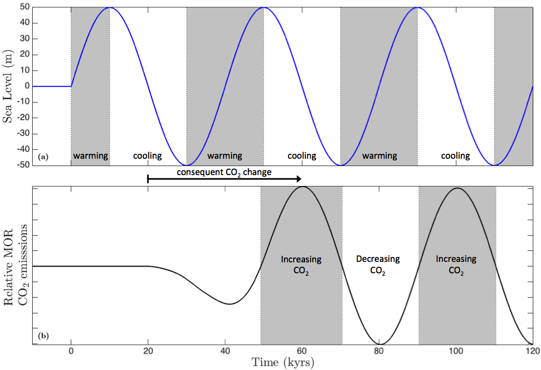
Figure 1: (a) Sinusoidal sea level change and (b) consequent global MOR $\text{CO}_{2}$ emissions for a 40 kyr lag (using Burley and Katz (2015) calculations the emissions are, roughly, proportional to minus the rate of change of sea-level offset by the lag time). Sea level is treated as an independent input in this figure. The grey shading denotes a warming climate in panel (a) and increasing $\text{CO}_{2}$ in panel (b). MOR $\text{CO}_{2}$ emissions oppose the SL change when grey regions overlap white regions between the two panels; MOR lag of 30–50 kyrs gives regimes that oppose 40 kyr sea level more than they reinforce it.

The lagged MOR $\text{CO}_{2}$ response’s effect on glacial cycles was first investigated in Huybers and Langmuir (2017) using coupled differential equations to parameterize global ice volume, average temperature, and atmospheric $\text{CO}_{2}$ concentration. Ice volume changes at a rate proportional to both the current temperature and ice volume to the third power (the latter gives a maximum and minimum bounding ice volume). Temperature varies according to insolation, temperature, and atmospheric $\text{CO}_{2}$ concentration. Atmospheric $\text{CO}_{2}$ concentration varies according to average temperature, subaerial volcanism and MOR volcanism (based on Burley and Katz (2015) calculations). These equations represent a coupled, non-linear oscillator, and generate glacial cycles at a multiple of the obliquity period.

These results are intriguing, however there are limits in their physical representation. For instance, they have: 1) an insolation forcing timeseries with no seasonal or spatial component; 2) a negative ice feedback proportional to the volume of the ice sheet cubed, inducing symmetrical variability rather than sawtooth behaviour; 3) no isostatic lithospheric response to the ice sheet. These simplifications remove potentially important physical mechanisms from the model glacial system.

These results are intriguing, however a more complete representation would allow more detailed consideration of the key physics. The present study builds on Huybers and Langmuir (2017) by extending the modelling framework to a low complexity earth system model. We ask: what properties the volcanic $\text{CO}_{2}$ response to glacial cycles must have to alter the period of a glacial cycle?

We extend a simplified climate model from Huybers and Tziperman (2008) which focused on accurate treatment of orbital forcing, using an Energy Balance Model (EBM) coupled with an ice sheet model. The EBM calculates daily insolation to resolve the counteracting effects of orbital precession on ice sheets: hotter but shorter summers. The Huybers and Tziperman (2008) model demonstrates 40 kyr glacial cycles in response to insolation forcing. To maintain their focus on orbital effects, they did not consider the radiative effects of varying atmospheric $\text{CO}_{2}$ and water vapour; they assumed an atmosphere of constant composition. From that framework we extend to a system of three component models: energy balance, ice sheet growth, and $\text{CO}_{2}$ concentration in the atmosphere. Our model does not aim to be perfect representation of the climate; rather it focuses on approximating key features and feedbacks such that we can calculate Earth’s glacial state over several glacial cycles.

Previous models of glacial cycles have ranged from simple, abstracted systems (Imbrie and Imbrie, 1980) to detailed representations of ice sheets and climate physics (Abe-Ouchi et al., 2013) — our model complexity is partway along this spectrum, considering the essential physics acting on a pseudo-2D system. However, even Abe-Ouchi et al. (2013) omit the carbon cycle, using imposed $\text{CO}_{2}$ concentrations rather than a dynamic system. No model has yet fully coupled an explicit representation of the solid-earth carbon cycle to physical representations of the Earth’s climate. This work presents such a fully coupled model using a low-complexity physical representation. The full insolation forcing is used to drive an Earth system response in $\text{CO}_{2}$ concentration, temperature, and ice sheet configuration.

We will show that this model, when forced by the observed $\text{CO}_{2}$ record, calculates sea-level timeseries that closely match the historical record. When $\text{CO}_{2}$ evolves freely, the model has no $\sim$100 kyr sea level variability until we include the lagged MOR $\text{CO}_{2}$ feedback; it is necessary to have a $\text{CO}_{2}$ feedback process with a period similar to or greater than the default 40 kyr glacial cycle in order to disrupt that cycle. We will show that the variation in MOR $\text{CO}_{2}$ emissions has the potential to generate sawtooth glacials.

The importance of volcanism in glacial cycles depends on both the percentage variations in volcanic emissions during glacial cycles and the background volcanic $\text{CO}_{2}$ emissions rate. There are uncertainties in both these quantities for MOR and subaerial systems. This uncertainty guides the modelling choices in made here. Rather than attempt a single exact estimate of global volcanic effects, we instead consider a range of volcanic effects. We define the threshold at which volcanism changes the pacing of glacial cycles, and compare this to estimates of these volcanic quantities. If the threshold values are orders of magnitude outside of estimates of these quantities, it would be strong evidence that volcanic $\text{CO}_{2}$ variability is not a important mechanism in glacial cycles. Our model scales linearly with changes in baseline volcanic emissions and volcanic variability, so our results can be readily reinterpreted if such estimates are updated.

As mentioned above, our preference in this work is to consider the Earth’s early-Pleistocene glacials as 40 kyr cycles with an internal Earth system feedback that locked the Earth into a 100 kyr mode after the mid-Pleistocene transition. The model system is agnostic about the orbital forcing responsible for this; our forcing includes the full insolation distribution in precession, obliquity, and eccentricity. Whilst it would be possible to parse the relative influence of obliquity and precession index forcing, it is not needed in the present context.

Section 2 introduces the three component models used to generate our results and discusses their coupling. Section 3 contains demonstrations of conceptually important model behaviour and the key model results: Section 3.1 discusses how sea level period controls the maximum atmospheric $\text{CO}_{2}$ anomaly induced by MOR volcanoes. Section 3.2 demonstates our model’s agreement with historical sea-level data when forced by the ice core $\text{CO}_{2}$ record. Section 4.1 investigates the climate effects of different MOR lag times under simplified orbital forcing and discusses the importance of different timescale $\text{CO}_{2}$ feedbacks. Section 4.2 demonstrates model behaviour for a range of potential $\text{CO}_{2}$ feedbacks, showing the circumstances under which $\sim$100 kyr cycles occur. Section 5 discusses the significance of assumptions and simplifications made in the model and the meaning of our results. Section 6 summarises our findings and offers some conclusions.

2 Method

The research question we ask, regarding the pacing of glacial cycles, requires that the model must run for 100’s of thousands of years. To be capable of this, the model must use a reduced complexity representation of the climate system.

The model treats the Earth’s climate as a record of ice sheet volume (equivalently, sea level), temperature, and the $\text{CO}_{2}$ concentration in the atmosphere. We consider 2D models of ice and temperature, modelling a line from the equator to north pole.

Independent variables are time $t$ and latitude $\phi$. Temperature $T$ is a function of $t,\phi$, changing due to insolation $S$, ice (i.e., surface albedo), atmospheric $\text{CO}_{2}$ concentration, current temperature (controls longwave infrared emissions), and the temperature gradient with latitude. Ice sheet thickness $h$ is a function of $t,\phi$. It changes as ice flows under its own weight and accumulates/melts according to local temperature. Integrating $h$ over latitude $\phi$ — with an assumed ice sheet width — gives total ice volume $V$. The $\text{CO}_{2}$ concentration in the atmosphere $C$ is a function of $t$, varying in response to three processes: $T$-dependent changes in the surface system (i.e., atmosphere, biosphere, and ocean) partitioning of $\text{CO}_{2}$, $V$-dependent changes in subaerial volcanism (SAV), and $V$-dependent changes in mid-ocean ridge (MOR) volcanism. The dependencies of these components are shown graphically in figure 2.

These components are described by the following differential equations

$$\dfrac{\partial{T(t,\phi)}}{\partial{t}} =f_{T}\left(S,h,C,T,\dfrac{\partial{T}}{\partial{\phi}}\right)\;\;,$$ (1)

$$\dfrac{\partial{h(t,\phi)}}{\partial{t}} =f_{h}\left(\dfrac{\partial{h}}{\partial{\phi}},T\right)\;\;,$$ (2)

$$\dfrac{\text{d}{C(t)}}{\text{d}{t}} =f_{C}\left(\dfrac{\partial{T}}{\partial{t}},\dfrac{\text{d}{V}}{\text{d}{t}}\right)\;\;,$$ (3)

where functions $f_{i}$ determine the rate of change of variable $i$. The system of equations (1)–(3) is driven by variation in insolation, $S$, computed using Berger and Loutre (1991). All other variables evolve in response to the internal state of the model. Conceptually, this matches the Earth system: internal dynamics affected by the external driving force of variable insolation.

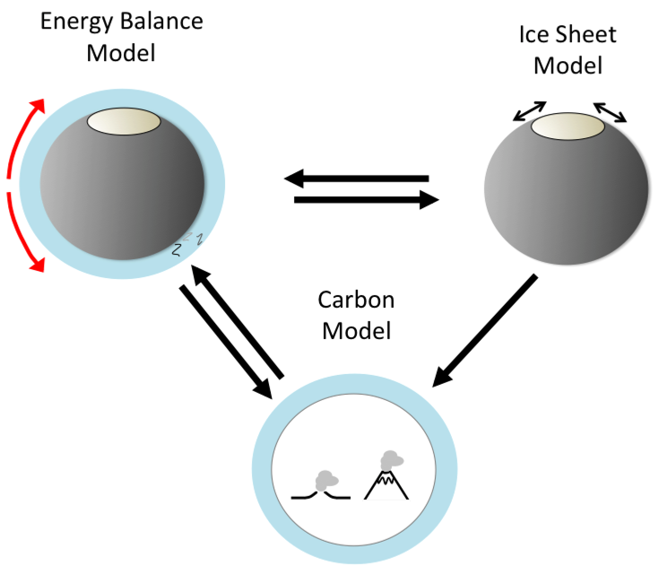
Figure 2: Component models and their interactions. Black arrows between models show information flow. Energy balance (i.e., temperature) is affected by carbon concentration in the atmosphere and the extent of the ice sheet. The ice sheet is affected by temperature only. Carbon concentration in the atmosphere is affected by the rate of change of temperature and sea level (determined by the ice sheet).

Having discussed the way these component models will be linked, we now describe each model in detail.

2.1 Energy Balance Model

To calculate planetary temperature and the annual ice accumulation/melting we use an Energy Balance Model (EBM) based on Huybers and Tziperman (2008). This model calculates insolation (and consequent temperature changes) at daily intervals, thus explicitly modelling the seasonal cycle and its effect on ice sheet accumulation/melting. Importantly, this includes the counteracting effects of orbital precession on ice sheets: hotter but shorter summers.

The EBM is fully detailed in Huybers and Tziperman (2008), here we will briefly cover the overall model and explain our method for including radiative forcings to represent $\text{CO}_{2}$, water vapour, lapse rate, and cloud effects.

The EBM tracks energy in the atmosphere, ground surface, and subsurface; this is encompassed in:

$$c_{a}\dfrac{\partial{T_{a}}}{\partial{t}}=S_{a}+I_{a}+F_{s}+D_{a}\;\;,$$ (4)

$$c_{s}\dfrac{\partial{T_{s}}}{\partial{t}}=S_{s}+I_{s}-F_{s}+F_{ss}\;\;,$$ (5)

$$c_{ss}\dfrac{\partial{T_{ss}}}{\partial{t}}=-F_{ss}\;\;,$$ (6)

where $a,s,ss$ subscripts denote atmospheric, surface and subsurface quantities respectively, $c$ is heat capacity (Jm^-2K^-1), $S$ is the solar radiation (shortwave), $I$ is net infrared longwave radiation, $F$ is sensible heat flux (W/m^-2), and $D_{a}$ is meridional heat flux. See table 2 for parameter values.

We modify this EBM to include radiative forcings from atmospheric composition and a temperature-dependent precipitation, detailed in A.2. The atmospheric composition forcings represent $\text{CO}_{2}$, water vapour, lapse rate, and cloud effects. These radiative forcings are treated with two terms: one for the $\text{CO}_{2}$ forcing, and another for the aggregate effects of water vapour, lapse rate and cloud forcings. Both terms are changes in the mean height at which the atmosphere becomes transparent to longwave radiation and emits to space, thus adjusting the longwave energy balance.

The net longwave radiation balance of the atmosphere $I_{a}$ has three terms representing, respectively, the longwave emissions from the ground (absorbed by the atmosphere), emissions from the atmosphere to the ground, and emissions from the atmosphere into space. Applying the collective radiative forcings to $I_{a}$ gives

$$I_{a}=\sigma T^{4}_{s}-\big{(}\epsilon_{a}\sigma\big{(}T_{a}-\Gamma_{m}H_{as}\big{)}^{4}+R_{\textrm{DLW}}\big{)}-\>\>\epsilon_{a}\sigma\big{(}T_{a}+\Gamma_{m}(H_{ul}+\Delta z_{C}+\Delta z_{\textrm{WLC}})\big{)}^{4}\;\;,$$ (7)

where $\sigma$ is the Stefan-Boltzmann constant, $\epsilon_{a}$ is atmospheric emissivity, $T_{a}$ is the temperature of the middle atmosphere, $\Gamma_{m}$ is the temperature profile in the atmosphere $\textrm{d}T/\textrm{d}z$, $H_{as}$ is the middle-atmosphere-to-surface height, $H_{ul}$ is the default middle-atmosphere-to-upper-layer height, $\Delta z_{C}$ is the change in upper layer height due to $\text{CO}_{2}$ concentration in the atmosphere, and $\Delta z_{\textrm{WLC}}$ the change in upper layer height modelling the parameterised water vapour, lapse rate, and cloud feebacks.

To validate this reformulation of the Huybers and Tziperman (2008) EBM, we compare our model against present-day climate, and perform a $\text{CO}_{2}$-doubling experiment.

Figure 3 shows our model’s calculation of preindustrial conditions and the average surface temperature for 1950-80 (Berkeley Earth Surface Temperatures, ). To approximate our model’s land-only, zero-relief Earth, the land temperatures are on a transect of data points closest to 52E — a continental regime with minimal ocean influence and low relief. Annual mean, maximum, and minimum temperatures are well aligned between our model and the data. The largest errors are near the equator, presumably owing to our model lacking latent heat transport, Hadley cell circulation, a representation of the low land fraction near the equator ( i.e., no longitudinal heat transport) and because of our no-flux equatorial boundary condition. However, the seasonal temperature range is accurately captured across latitudes (except the polar coast, where oceanic buffering effects slightly reduce the annual temperature range), and the mean model temperature is within 1 K of the observed record at the high latitudes (55-75N) most relevant to ice sheet dynamics.

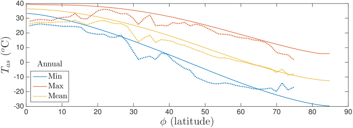
Figure 3: Annual mean, maximum, and minimum surface air temperatures for our model (solid lines) and average 1950-80 land data (dashed lines) (Berkeley Earth Surface Temperatures, ). Model uses fixed modern insolation, and preindustrial $\text{CO}_{2}$ concentration. Temperature data is based on a transect of land points closest to 52E. This representative transect was chosen as it is low-elevation land, removed from oceanic influences, thus replicating our zero relief, ocean-free EBM. Furthermore, this region hosted at ice sheet at the LGM.

Figure 4 shows an experiment in which we double $\text{CO}_{2}$ from preindustrial conditions, holding atmospheric $\text{CO}_{2}$ concentration constant and running the model to equilibrium temperature. We calculate an increase in annual global average atmospheric temperature of 3.7 K; placing our model within the range of GCM predictions for $\text{CO}_{2}$-doubling. However, we do not match the some features of the change in temperature with latitude in GCMs. 1) Temperature anomalies around the ascending/descending arms of atmospheric circulation cells, and 2) Large polar amplification, driven by vast reduction in arctic sea-ice (Rind et al., 1995). However, recent interglacials are not thought to remove arctic sea ice, so this difference is not important in modelling late-Pleistocene glacial cycles.

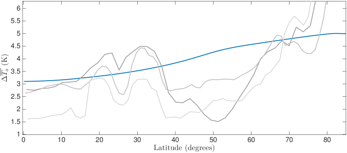
Figure 4: Change in annual average atmosphere temperature for a doubling of $\text{CO}_{2}$ from 280 to 560 ppmv under ice-free conditions with present-day insolation in our model (blue) and for $\text{CO}_{2}$-doubling experiments in CMIP3 (grey). From dark to light grey these are ECHAM, miroc 3.2, and hadgem1; to reduce noise, data shown is the difference between the initial and final five years of the CMIP models. CMIP data is taken along the same transect as in figure 3.

Finally, the EBM includes an ice melting scheme (detailed in Huybers and Tziperman (2008)) — whereby if ice-covered ground reaches $0^{\circ}$C, ice melts according to the available thermal energy — giving the annual ice accumulation/melting at each latitude, an input for our ice sheet model.

2.2 Ice Sheet Model

Conceptually, our ice model combines the EBM’s annual ice accumulation/melting with ice flow under gravity and isostatic bedrock adjustments. We calculate both the evolution of ice thickness across latitudes $h(t,\phi)$ and the global ice volume $V(t)$. The former is used by the EBM for ground height and reflectivity, and the latter is used to calculate volcanic responses to glaciation and sea level.

We use a vertically-integrated 1D model for $h$, following the Huybers and Tziperman (2008) model exactly, except we use a higher grid resolution and smaller timesteps. This ice model calculates the thickness of a northern hemisphere ice sheet flowing according to Glen’s Law, with an accumulation or ablation of ice at each latitude calculated according to the EBM. It assumes incompressible ice, temperature-independent ice deformability, and the ‘shallow ice’ approximation whereby deformation is resisted only by horizontal shear stress, including basal stress. The ground surface is initially flat, and deforms to maintain local isostatic equilibrium in each gridcell. Basal sliding is included via a shearable sediment layer, such that the base of the ice sheet can move with respect to the bedrock. Full details for calculating $h$ can be found in Huybers and Tziperman (2008), and for completeness we state the equations and parameter values in appendix A.5.

We calculate ice volume from the vertically-integrated 1D ice model by assuming that ice sheet width is 60% of Earth’s circumference at each latitude $\phi$ — a reasonable approximation at high northern latitudes. Ice volume is expressed in eustatic meters sea-level equivalent (msle) by dividing ice sheet volume by the ratio of ice to water density and the surface area of the ocean. Over glacial cycles, thermal expansion of the oceans is negligible at $<1$% of glacial sea level change (McKay et al., 2011) and we ignore it in our sea level calculation.

2.3 Carbon Model

The last component of our model calulates the $\text{CO}_{2}$ concentration in the atmosphere over time, responding to changes in climate configuration and volcanic emissions. We will consider the $\text{CO}_{2}$ influences in turn, and discuss their timescale and magnitudes.

Glacial–interglacial $\text{CO}_{2}$ variations are not fully understood, and certainly cannot be replicated from first principles. Therefore we circumvent the accounting of all sources and sinks of $\text{CO}_{2}$. We instead parameterise atmospheric $\text{CO}_{2}$ concentration, $C$, as proportional to average global temperature, matching a well-established feature of reconstructed Pleistocene climate records (Cuffey and Vimeux, 2001; Sigman et al., 2010).

This carbon–temperature feedback accounts for all potential feedbacks in the surface carbon system, such as ocean-atmosphere equilibration and biosphere changes, and aggregates them to a single feedback parameter. This simplification allows us to be agnostic about the causes of these $\text{CO}_{2}$ changes and to enforce agreement with the observed correlation between $\text{CO}_{2}$ and ice volume in the Pleistocene. However, it fails to capture, for example, state dependency (a Kelvin change in average planetary temperature changes atmospheric $\text{CO}_{2}$ by a fixed amount, regardless of the current temperature). This may be important given recent suggestions of a lower limit on $C$ during glacial cycles (Galbraith and Eggleston, 2017) and several plausible non-linear components partitioning $\text{CO}_{2}$ in the surface system. These include, but are not limited to, hysteresis in the ocean overturning circulation (Weber et al., 2007), iron fertilisation (Watson et al., 2000), plant growth being non-linearly temperature dependent, and seafloor and permafrost methane clathrate release (MacDonald, 1990). Despite these complications, the overall linear $C,T$ relationship in the Pleistocene suggests our formulation is a good representation of leading order behaviour.

We also include changes to atmospheric $\text{CO}_{2}$ from volcanic emissions as separate, independent terms, giving a carbon equation:

$$\dfrac{\partial{C(t)}}{\partial{t}}=\gamma_{\textrm{T}}\dfrac{\partial{\overline{T}_{s}}}{\partial{t}}+\gamma_{\textrm{MOR}}\;f_{\textrm{MOR}}\left(\dfrac{\partial{V}}{\partial{t}}\right)+\gamma_{\textrm{SAV}}\;f_{\textrm{SAV}}\left(\dfrac{\partial{V}}{\partial{t}}\right)\;\;,$$ (8)

where $f_{\textrm{SAV}},f_{\textrm{MOR}}$ are functions that map sea level history to current $\text{CO}_{2}$ emissions for global subaerial and mid-ocean ridge volcanism respectively. The $\gamma_{i}$ are coefficients that represent the sensitivity of $C$ to changes in the Earth system. The $\gamma_{\textrm{T}}$ term denotes the sensitivity to changes in surface temperature; this is interpreted physically as the net effect of surface system (i.e., atmosphere, biosphere, and ocean) partitioning of $\text{CO}_{2}$ between the atmosphere and other reservoirs. $\gamma_{\textrm{T}}$ has units of $\text{CO}_{2}$ mass per Kelvin change in (annual and spatial) average planetary temperature, stated in ppmv/K for convenience (7.81 Gt$\text{CO}_{2}$ = 1 ppmv change in atmospheric $\text{CO}_{2}$ concentration). The $\gamma_{\textrm{MOR}}$ and $\gamma_{\textrm{SAV}}$ coefficients are $C$ sensitivity to changes in sea level caused by variable MOR and subaerial volcanic $\text{CO}_{2}$ emissions. These coefficients state the peak change in annual volcanic $\text{CO}_{2}$ emissions resulting from a given rate of sea level change, and thus have units of Mtonnes $\text{CO}_{2}$ per year per cm/yr change in sea level.

Volcanic $\text{CO}_{2}$ emissions have distinct timescales for subaerial and MOR volcanic systems. MOR $\text{CO}_{2}$ emissions, according to modelling by two of the authors (Burley and Katz, 2015), respond to glacial sea-level change with a tens-of-thousands-of-years lag. Subaerial volcanism responds comparatively fast to changes in nearby ice sheets, with field evidence (Rawson et al., 2015; Kutterolf et al., 2013) showing responses in approximately 4 kyrs.

As shown in figure 5, we use an approximate Green’s function representation of each system where the rate of change of global ice volume (directly proportional to sea level) produces a change in $\text{CO}_{2}$ emissions at a later time. The $\gamma_{\textrm{MOR}}$ and $\gamma_{\textrm{SAV}}$ coefficients scale the height of these Green’s functions. The reasoning behind the imposed temporal patterns and magnitude of volcanic response is explained below.

The MOR Green’s function follows the global MOR results in Burley and Katz (2015). There are no published observational constraints on MOR $\text{CO}_{2}$ response to glaciation that can support or reject this model. However, records of sea-floor bathymetry are consistent with a sea-level-driven MOR eruption volume model (Crowley et al., 2015) that shares many features with the Burley and Katz (2015) model (though see Olive et al. (2015)).

In Burley and Katz (2015) sea-level change causes a $\text{CO}_{2}$ anomaly in mantle melt at about $60$ km depth below the MOR. This $\text{CO}_{2}$ anomaly is subsequently carried by magma to the MOR axis. The MOR Green’s function’s magnitude and lag time are determined by the mantle permeability $K_{0}$, a physical property that controls how quickly mantle melt percolates through the residual (solid) mantle grains. The mantle permeabilities assumed in this paper are within the accepted range (Connolly et al., 2009), and give $\text{CO}_{2}$ travel times in agreement with the ²³⁰Th disequilibria in MORB (Jull et al., 2002).

Figure 5c shows example MOR $\text{CO}_{2}$ emissions responses for a range of mantle permeabilities. They show similar features: a decrease in $\text{CO}_{2}$ emissions lasting 10s-of-kyrs that lags the causative sea-level increase by 10s-of-kyrs. The total change in $\text{CO}_{2}$ emissions (i.e., the integral of figure 5c) is the same for all permeabilities.

In subsequent sections, we discuss behaviour in terms of the ‘MOR lag’ rather than mantle permeability, as the former has a more direct interpretation that is relatable to other model components (as in fig 1).

MOR $\text{CO}_{2}$ emissions dissolve into intermediate ocean waters, delaying entry into the atmosphere by a few hundred years. This delay is much smaller than both the MOR lag time and the uncertainties therein; hence we neglect it.

The SAV Green’s function has a temporal pattern based on the observation-derived eruption volume calculations in Rawson et al. (2015, 2016); these show a large increase in eruptive volume per unit time (volume flow rate) 3–5 kyrs after deglaciation, followed by a few kyrs of low eruptive volume per unit time, then a return to baseline activity. This timing is consistent with other studies that report an increase of subaerial arc volcanism that lags behind deglaciation by $\sim$$4$ kyrs (Jellinek et al., 2004; Kutterolf et al., 2013). Therefore, the volume-flow-rate timeseries of Rawson et al. (2015) represents the temporal response of SAV accurately.

However, this is the response of a single volcano, and we need to model the global volcanic system. The planet’s volcanoes experience different glacial coverage during an ice age, so the change in a single volcano’s volume-flow-rate is not a valid basis for a global aggregate. Therefore, we want to adjust the magnitude of volume-flow-rate change, while keeping the temporal response pattern.

We create a representative global value for the volume-flow-rate change by using the eruption frequency datasets of Siebert et al. (2002) and Bryson et al. (2006), as compiled in Huybers (2011). To do this, we assume that eruption frequency is proportional to eruptive volume per unit time. This is an oversimplification, however eruption frequency is the only available constraint on global subaerial volcanic behaviour over a glacial cycle (erosion, reworking, and burial of volcanic units causes great difficulties in eruption volume calculations prior to the past few thousand years). Eruption frequency increases by at least $\sim$50% during deglaciation. Next, we consider how to calculate the SAV $\text{CO}_{2}$ emissions.

To relate SAV eruption volume per unit time to $\text{CO}_{2}$ emissions there are three regimes to consider: if increased SAV volcanic eruption volume during deglaciation is entirely due to venting of pre-existing magma reservoirs, there would be direct proportionality between $\text{CO}_{2}$ flux and eruption volume; at the other extreme, if the eruption-volume increase is entirely due to enhanced melting of a $\text{CO}_{2}$-depleted mantle there is, to leading order, no correlation between eruption volume and $\text{CO}_{2}$ flux (see Burley and Katz (2015) appendix A.4). Finally, if there is variable melting of a carbon-bearing phase (either mantle or metamorphism of a crustal rock unit (Goff et al., 2001)) there will be a correlation between eruption volume and $\text{CO}_{2}$, but of unknown strength and with a dependence on location. For lack of information to guide us, we model SAV $\text{CO}_{2}$ emissions as directly correlated to the rate-of-change of ice volume. This leaves considerable uncertainty in the coefficient $\gamma_{\textrm{SAV}}$.

Finally in volcanism, it is unclear if hotspots have a glacially-driven variability. Their deep melting systems (Harðardóttir et al., 2017; Yuan and Romanowicz, 2017; Zhao, 2001) preclude sea-level and glaciation influencing depth-of-melt-segregation as at MORs. Instead, hotspots’ extensive magma chamber systems (Harðardóttir et al., 2017; Larsen et al., 2001) imply they respond like SAV. This is consistent with the observed volume flow rate in Iceland (Maclennan et al., 2002) (although other mechanisms could also be consistent with the data). We expect hotspots respond on the same timescale as arc volcanoes; however, most hotspots are oceanic thus the pressure change will be caused by sea level rather than ice sheets. Thus hotspots (if they have any glacially-driven $\text{CO}_{2}$ variability) will be a negative feedback acting simultaneously with arc volcanism, thus increasing the uncertainty in the appropriate value of $\gamma_{\textrm{SAV}}$.

Above, we have described the logic leading to our Green’s function representations of MOR and subaerial volcanism. The physics-driven and data-driven calculations in this logic prescribe the percentage change in $\text{CO}_{2}$ emissions in response to rate-of-sea-level-change. We multiply the percentage value by the average annual volcanic emissions to get Green’s functions in units of Mt$\text{CO}_{2}$/year per cm/yr. Therefore, the Green’s functions’ magnitudes have uncertainty from both the calculated percentage change and the default emissions value.

Annual MOR $\text{CO}_{2}$ emissions have large uncertainties, with papers stating 2-standard-deviation lower bounds of 15–46 Mt$\text{CO}_{2}$/yr, and upper bounds of 88–338 Mt$\text{CO}_{2}$/yr from geochemical analyses (Marty and Tolstikhin, 1998; Resing et al., 2004; Cartigny et al., 2008; Dasgupta and Hirschmann, 2010). The most recent estimates by Le Voyer et al. (2017) are MOR $\text{CO}_{2}$ emissions of 18–141 Mt$\text{CO}_{2}$/yr. The $91$ Mt$\text{CO}_{2}$/yr estimate used in Burley and Katz (2015) is fairly central in that range and for consistency I continue to use that value in this thesis.

Annual SAV $\text{CO}_{2}$ emissions are also uncertain. Studies estimate SAV $\text{CO}_{2}$ emissions are within $\pm 15$% of MOR $\text{CO}_{2}$ emissions (Marty and Tolstikhin, 1998; FISCHER, 2008), much less than the uncertainty in each value. For simplicity, we set background SAV $\text{CO}_{2}$ emissions as equal to MOR $\text{CO}_{2}$ emissions.

We assume that the solid Earth has no net effect on atmospheric concentration of $\text{CO}_{2}$, $C$, over the late Pleistocene, and therefore when SAV or MOR volcanism are at baseline emissions (i.e., $0\%$ in figure 5(b,c)) they do not affect $C$. Any increase or decrease from average volcanic $\text{CO}_{2}$ emissions acts to increase or decrease $C$. Physically, this assumes the weathering drawdown of $\text{CO}_{2}$ balances the time-average of volcanic emissions, and that any variations in the weathering rate are at the sub-ka timescale (captured by $\gamma_{\textrm{T}}$) or negligible on the 1 Ma timescale.

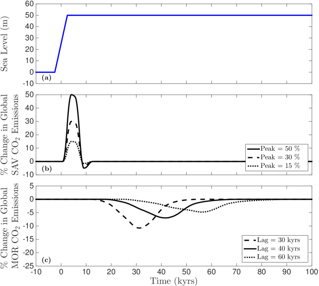
Figure 5: Toy deglaciation event with plots of (a) sea level, and the consequent $\text{CO}_{2}$ emissions of (b) subaerial and (c) MOR volcanism. $\gamma_{\textrm{MOR}}$ and $\gamma_{\textrm{SAV}}$ set the peak values of the emissions in panels (b),(c). The integrals of $\text{CO}_{2}$ emissions curves in panel (c) are all equal.

The volcanic Green’s functions assume that all volcanic $\text{CO}_{2}$ variations directly change $\text{CO}_{2}$ concentration in the atmosphere. However, we might expect, for example, an extra 5 Mt/yr of volcanic $\text{CO}_{2}$ to be partially absorbed by the ocean such that atmospheric $\text{CO}_{2}$ mass does not increase at 5 Mt/yr. For modern oceans it is calculated that $15$–$30\%$ of $\text{CO}_{2}$ added to the atmosphere remains after 2 kyrs (Archer et al., 2009). However, such calculations are state dependent; both the decay timescale and equilibrium airborne fraction vary with the injected $\text{CO}_{2}$ mass and the initial ocean state. There are no estimates of the decay timescale or equilibrium airborne fraction on glacial timescales, nor glacial–interglacial ocean models from which one could be extracted. For simplicity, plots in this paper assume that all volcanic $\text{CO}_{2}$ remains in the atmosphere, however it is perhaps fairer to discount emissions by a constant factor — this discount is discussed in the conlusions section in terms of the of volcanic emissions required for certain climate behaviour.

Finally, we highlight a feature of the volcanic response that is important for understanding $C$ evolution over time in equation (8): the total change in MOR $\text{CO}_{2}$ emitted (the integral of curves in figure 5c) is directly proportional to the amplitude of sea level change (Burley and Katz, 2015).

Therefore the amplitude of changes in atmospheric $\text{CO}_{2}$ concentration $\Delta C$ caused by volcanism, for a single change in sea-level, are directly proportional to the amplitude of sea-level changes $\Delta V$ (section 3.1 illustrates the more complex scenario of periodic sea-level). By comparison, $C$ changes due to surface system feedbacks are proportional to changes in mean atmospheric temperature $\bar{T}$. $C$ determines radiative $\text{CO}_{2}$ forcing and thus this forcing depends upon past variations in ice volume $V$ and $\bar{T}$. Furthermore, the effective insolation forcing depends on planetary albedo (i.e., ice sheet extent). Consequently, the balance of climate forcings in the model varies as the amplitude of changes in ice sheet volume, extent, and mean atmospheric temperature vary.

Note that we only model a single variable volcanic process — $\text{CO}_{2}$ emissions — yet other glacially-driven volcanic changes could affect climate. For instance: 1) SAV aerosol emissions will increase following deglaciation. This could be a positive or negative climate feedback depending on injection height, particle size and composition distributions — all poorly constrained even for current volcanic systems. 2) MORs will have varying emissions of many chemical species in response to glacial cycles, $\text{CO}_{2}$ only represents the end-member of highly incompatible species (partitions strongly into mantle melt), with less incompatible species having a shorter lag and smaller variation than $\text{CO}_{2}$. Some species, like bio-active Fe or those that may affect ocean pH, could be relevant to global climate. 3) MOR hydrothermal systems vary with glacial cycles (Lund and Asimow, 2011; Middleton et al., 2016). Increased melt productivity at MORs would presumably drive more vigorous convection of seawater in the hydrothermal system. However, the net effect of increased circulation is hard to predict due to the complex chemical and biological processes acting on fluid composition.

These potential glacially-driven volcanic effects have large uncertainty and complex underlying physical processes. We choose to not include them; they would increase model complexity and lead to an excess of uncertain parameters with overlapping timescales.

Having defined the component models, we now describe the coupling between these components and how the combined model is initialised.

2.4 Coupling and Initialising the Model

The three component models operate on different timescales and hence it is not immediately clear how to best couple them together. Careful consideration of timescales will inform our choice.

The fastest changes in the model are the seasonal changes in insolation and temperature, setting the shortest timestep in the model at $10^{-2}$ years. Taking such small timesteps for a full million years would be prohibitively expensive, so we use the simplification that $1)$ annual averages of thermal quantities are accurate drivers of ice sheet flow and carbon change (for example, we calculate ice sheet growth using the annual average melting/accummulation rate), and $2)$ subsequent years are very similar. Consequently we use the EBM model to calculate the equilibrium temperature and precipitation/melting distribution for the current $\text{CO}_{2}$ concentration and ice sheet configuration. We then hold temperature and precipitation constant while running the carbon and ice sheet models. After small changes in $C$ and ice configuration we run the EBM again, calculating a new temperature and precipitation/melting distribution to drive further changes in $C$ and ice.

The timescale for these ‘small changes’ in ice and $C$ will clearly be greater than a year. In testing the model, we found a timescale on the order of $200$ years was suitable. Shorter timescales do not alter $V$ or $C$ significantly.

For the results presented here, the ice model was run for intervals of 250 years, with two-year timesteps. The carbon concentration in the atmosphere is updated every 250 years, then the EBM is run for five years to update the temperature and precipitation/melting distribution in preparation for continuing the ice model. To initialise the model at a particular time in the past, the insolation is computed for that time. The $\text{CO}_{2}$ concentration is taken from ice core data. These are both held constant while the EBM and ice sheet come into equilbrium. Subsequently, the model is advanced using the timestepping described above.

The range of fully-defined initialisation times are limited by the atmospheric $\text{CO}_{2}$ record, which extends back $800$ kyrs (Bereiter et al., 2015) (insolation is well defined for 10s-of-Myrs (Berger and Loutre, 1991; Laskar et al., 2004)).

We could use earlier start times by solving an inverse problem to define starting $C$: use a range of initial $C$ values and match the resulting equilibrium ice sheet volume to a proxy sea-level record. However the difficulties and objections such a method raises would distract from the core investigation of this paper.

3 Results: Basic Model Behaviour

3.1 Mid-ocean ridge CO₂ response to sinusoidal sea level

This section demonstrates how global MOR CO₂ emissions respond to sinusoidal sea-level changes, neglecting climate feedbacks from that $\text{CO}_{2}$ change.

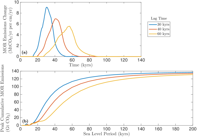
Figure 6: MOR CO₂ emissions driven by sinusoidal sea level of 50 m amplitude, no climate feedbacks. Panel (a) shows Green’s functions for the global MOR system with different lag times; stated as the global MOR emissions change in MtCO₂/yr per cm/yr rate-of-change in sea level. The $\gamma_{\textrm{MOR}}$ values are those predicted from Burley and Katz (2015) for the lag times shown: 9.2, 7.1, 5.6 Mt$\text{CO}_{2}$/yr per cm/yr rate-of-change of sea-level. Panel (b) shows the maximum cumulative MOR CO₂ emissions. 7.81 Gt$\text{CO}_{2}$ = 1 ppmv $C$ change, so maximum values in panel (b) are equivalent to 18 ppmv.

As shown in figure 1, sinusoidal sea-level causes a sinusoidal variability in relative MOR CO₂ emissions rate (Mt $\text{CO}_{2}$ per year relative to baseline MOR emissions). When these relative $\text{CO}_{2}$ emissions are positive, MORs are increasing the $\text{CO}_{2}$ concentration in the atmosphere; when negative, $\text{CO}_{2}$ concentration in the atmosphere is decreasing. Therefore, taking the integral (with respect to $t$) of the relative MOR $\text{CO}_{2}$ emissions rate gives the total change in atmospheric $\text{CO}_{2}$ mass caused by MORs, which is also sinusoidal. The peak-to-trough magnitude of this sinusoid (after a transient windup period) is the ‘maximum cumulative MOR CO₂ emissions’ — the maximum $\text{CO}_{2}$ mass that variable $\text{CO}_{2}$ emissions add the atmosphere.

Figure 6b shows maximum cumulative MOR CO₂ emissions across a range of sinusoidal sea-level periods, for the three MOR lag times shown in figure 6a. The maximum cumulative MOR CO₂ emissions vary with sinusoidal sea-level frequency, meaning that MOR $\text{CO}_{2}$ emissions can have significantly larger effects on $C$ if the period of sea level change increases. The physical reason for this behaviour is that the mantle melt (and associated $\text{CO}_{2}$ anomaly) arriving at the MOR at any given time is an amalgamation of mantle melts generated at the base of the melting region across a range of times (the width of the Green’s functions in figure 6a) in the past. If this range of times is greater than the sinusoidal sea-level period then $\text{CO}_{2}$ anomalies of opposing effect arrive at the MOR simultaneously, reducing variability in MOR $\text{CO}_{2}$ emissions (see Burley and Katz (2015)). Therefore, as shown in figure 6, sinusoidal sea-level periods shorter than the Green’s function width cause small amplitude cumulative MOR CO₂ emissions.

For sinusoidal sea-level periods much larger than the Green’s function width, the cumulative MOR CO₂ emissions reach a constant value. When sea level falls, the depth of first melting under the MOR increases, creating new melt in a deeper section of mantle, and extracting the carbon from that mantle. The change in depth of first melting (and thus the volume of mantle decarbonated) is proportional to the amplitude of sea-level change. Therefore the maximum possible $\text{CO}_{2}$ injected into the atmosphere is determined by the amplitude of sea-level change, and different period sinusoidal-sea-levels have different effectiveness at reaching this maximum. Sea-level periods much longer than the Green’s function width allow this mantle volume to degas its carbon and emit $\text{CO}_{2}$ from the MOR without interference from opposing $\text{CO}_{2}$ anomalies. Thus longer sea-level periods converge to the maximum possible $\text{CO}_{2}$ release into the atmosphere.

Our arguments above state that maximum cumulative MOR $\text{CO}_{2}$ emissions will have near-zero values for sea-level periods much less than the width of the MOR Green’s function, and converge to a large value for sea-level periods greater than the width of the MOR Green’s function. The widths of our Green’s functions in figure 6a are approximately $30$–$60$ kyrs and, consequently, figure 6b demonstrates significant changes in the amplitude of cumulative emissions over glacial-cycle-relevant changes in sea-level period. For example, MOR systems with 40 kyr lag driven by 40, 80, 120 kyr sea-level period have maximum cumulative emissions of 64, 104, 126 Gt $\text{CO}_{2}$, corresponding to a doubling of MOR-derived $\text{CO}_{2}$ deviations when sea level changes from early-Pleistocene to late-Pleistocene periodicity.

This result is robust for any MOR system with a lag likely to destabilise 40 kyr glacial cycles (30–50 kyr): 1.4–$2.5\times$ increases in maximum cumulative MOR CO₂ emissions if sea level periodicity increases to $\sim$100 kyrs. See appendix A.6 for generalised mathematical treatment. Whilst MOR $\text{CO}_{2}$ emissions remain a small part of the overall glacial $\text{CO}_{2}$ cycles, this is a mechanism for MOR volcanism to reinforce $\sim$100 kyr glacial cycles if they occur.

Our SAV Green’s function width is 3.5 kyrs, much less than glacial sea-level periods, thus our calculated cumulative SAV $\text{CO}_{2}$ emissions do not vary significantly with sea-level period.

3.2 Forcing with historical CO₂ values

In this section we consider a forcing based on reconstructed atmospheric $\text{CO}_{2}$ concentration, $C$, and insolation. For this scenario $C$ is set to ice core values, rather than evolving according to equation (8). The scenario has two purposes: 1) validating our EBM and ice sheet model — the calculated ice sheet volume $V$ should approximate reconstructed sea-level data, and 2) demonstrating our model’s $V$ response to $\sim$$100$ kyr $C$ cycles — a benchmark for $V$ when subsequent sections calculate $C$ according to equation (8). These are both discussed below.

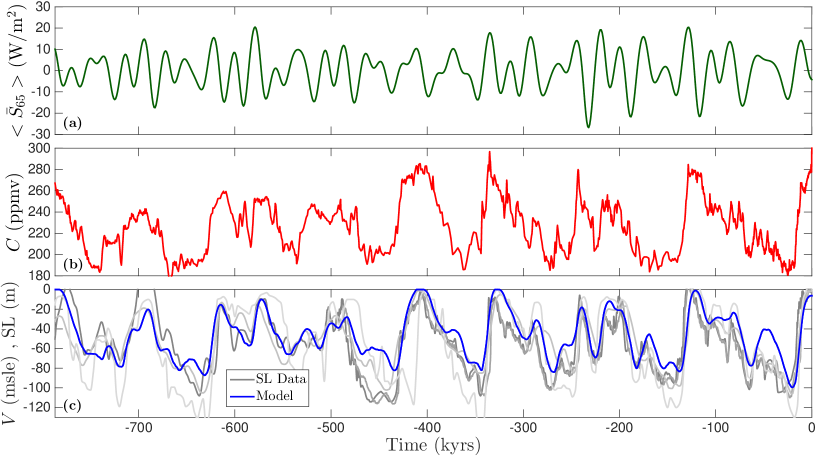
Figure 7: Model driven by insolation and ice core $\text{CO}_{2}$ values. Panel (a) shows mean summer half-year insolation at 65^∘N as deviation from the mean (Berger and Loutre, 1991). Panel (b) shows atmospheric $\text{CO}_{2}$ concentration (Bereiter et al., 2015). Panel (c) shows model ice volume $V$ in metres sea level equivalent and reconstructed sea level from several sources. From dark to light grey these are Rohling et al. (2009); Elderfield et al. (2012) as compiled in Martinez-Boti et al. (2015), maximum probability Red-Sea record from Grant et al. (2014), and the $\delta^{18}\textrm{O}$ record decomposed into a sea level component by van de Wal et al. (2011) and Siddall et al. (2010). Discrete Fourier transform of $V$ gives power of 49.5% at 80–120 kyr periodicity, 23.4% at 40 kyr periodicity and 5.6% at 23 kyr periodicity.

Figure 7a and 7b show the insolation and $C$ timeseries, and figure 7c shows the calculated ice volume $V$ (blue). Ice volume is correlated to both insolation and $C$, as expected. Furthermore, the calculated ice volume is a good fit to reconstructed sea-level records (grey). The model’s most significant difference from sea-level records is a lower variability at high frequencies; part of this difference is noise in the data but part is probably rapid changes in ice sheets that our model does not capture. Despite this, overall the timeseries in figure 7c are similar.

This similarity suggests the radiative forcings our model adds to Huybers and Tziperman (2008) are reasonable; we calculate realistic ice sheet configurations for actual insolation and $C$ values. There are uncertainties in our WLC radiative forcing parameter (water vapour, lapse rate and clouds — discussed in section A.4) due to the range in the tuning GCM cohort’s climate sensitivities. Across the plausible WLC forcing range, the maximum glacial varies from 75 m to 104 m. Changing WLC forcing does not introduce any novel model behaviour nor change the timing of turning points in $V$. Therefore we have confidence that our model behaviour is not contingent on peculiarly specific values of WLC forcing, and that our chosen value is physically plausible.

Figure 7c is a diagnostic for real-world glacial cycles in our model, demonstrating the ice volume timeseries that results from late-Pleistocene $C$ and insolation. Our model calculates powers in the ice volume timeseries, at the 23, 41, and $\sim$100 kyr periods of 5.6%, 23.4%, and 49.5% respectively, similar to the average of the displayed sea level data (4%, 10%, 55%). In section 4.2, we compare Fourier transforms of the ice volume timeseries from figure 7c and our full model system (forced purely by insolation, with $C$ determined by equation (8)).

3.3 Forcing with Individual Historical Values

Another useful benchmark of model behaviour is forcing with just the insolation (constant $\text{CO}_{2}$, 240 ppmv), and just the reconstructed atmospheric $\text{CO}_{2}$ concentration (constant insolation, 800 kyr average), and comparing to the result of section 3.2

In figure 8, our model calculates that $\text{CO}_{2}$ is the predominant influence on ice volume for the past 800 kyr (to be clear, this is not a statement of causality; an imposed $\text{CO}_{2}$ timeseries does not address the reason for that $\text{CO}_{2}$ variation). Table 1 quantifies this, showing that the power spectrum under both forcings is a weighted sum of, roughly, 70% $\text{CO}_{2}$-only and 30% insolation-only spectra.

This is a somewhat surprising result, as the calculations of W/m² forcing are significantly larger for insolation than $\text{CO}_{2}$ at the canonical 65N latitude ($\pm$15 W/m² for mean half-year insolation, $\pm$4 W/m² for $\text{CO}_{2}$). However, this is not an apples-to-apples comparison as $\text{CO}_{2}$ forcing is positive for the whole year, and insolation is highly seasonal. Furthermore, insolation at the top of the atmosphere is not the energy retained by the Earth system, which in our model is 43.7% of the top-of-atmosphere forcing for ice-covered ground (38.2% for non-icy ground, see section A.1), reducing the effective insolation forcing on the Earth system to 6.5 W/m², still $60$% larger than the $\text{CO}_{2}$ forcing.

This dominant $\text{CO}_{2}$ effect suggests an emergent property in the model whereby the year-round $\text{CO}_{2}$ forcing has a much larger effect on ice-sheets than mean half-year insolation of a similar magnitude. This could be due to a magnifying effect from year-round coherent forcing, or it could be that the 65N metric does not accurately reflect the forcing on ice sheets.

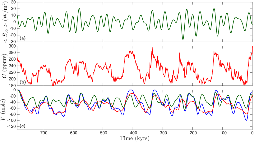
Figure 8: Model driven by insolation and ice core $\text{CO}_{2}$ values. Panels (a), (b) are identical to figure 7 — half-year insolation at 65N and atmospheric $\text{CO}_{2}$ concentration. Panel (c) shows model ice volume $V$ in metres sea level equivalent for both forcings (blue), $\text{CO}_{2}$-only (red) and Insolation-only (green).

Drivers	Power			Variance
	23 ka	40 ka	100 ka
Inso-only	14%	70%	3%	190
$\text{CO}_{2}$-only	1%	4%	67%	340
Both	6%	23%	50%	550

Table 1: Diagnostic values for ice volume timeseries in figure 8

4 Results: Volcanic Interactions

Having explored the basic behaviour of the model, we now show the effects of including volcanism and a dynamically varying $\text{CO}_{2}$ concentration to the model.

4.1 Varying mid-ocean ridge lag

In this section we determine which MOR lag times disrupt the $40$ kyr glacial cycles in the model, under simplified pure obliquity insolation forcing. This is a quantitative test of figure 1’s hypothesis that 30–50 kyr lags are capable of disrupting 40 kyr glacial cycles.

For this section, insolation is set to a 41 kyr sinusoidal obliquity variation, with eccentricity and precession fixed at their average values over the last 500 kyrs. Atmospheric $\text{CO}_{2}$ concentration is only affected by MOR $\text{CO}_{2}$ emissions; the temperature and subaerial-volcanism terms in eqn (8) are set to zero. However, the cumulative MOR $\text{CO}_{2}$ emissions change $C$ by about 9 ppmv for 100 m sinusoidal sea-level at 41 kyr (see figure 6b), far less than the 100 ppmv glacial–interglacial $C$ change. Therefore MOR sensitivity to sea-level $\gamma_{\textrm{MOR}}$ is increased to $10$$\times{}$ the values predicted in Burley and Katz (2015), facilitating $C$ change up to about 90 ppmv.

Figure 9a shows the changes in ice volume periodicity for different MOR lag times over a $1.64$ Myr model run, these results are presented as the power spectrum of ice volume (i.e., Discrete Fourier Transform ‘DFT’ of $V$). Figure 9b shows the final 300 kyrs of $V$ for a subset of these results. For lag times less than $20$ kyrs the $V$ cycle remains at 40 kyrs, phase-locked to the insolation forcing. Increasing lags across $20$–$35$ kyr gives the $V$ DFT a subsidiary peak at progressively longer periods. For 40 kyr lag time the $V$ cycle transitions to $80$ kyr cycles (80 kyr term is six times the power of $40$ kyr term). This transition occurs because there are low points in $C$ counteracting every second obliquity-driven deglaciation attempt, giving the ice volume timeseries shown in figure 9b. For lag times $>$$40$ kyr, $V$ cycles have about equal power between 40 kyr and a $>$$80$ kyr cycle. For a $60$ kyr MOR lag, there is a dominant cycle at $120$ kyr.

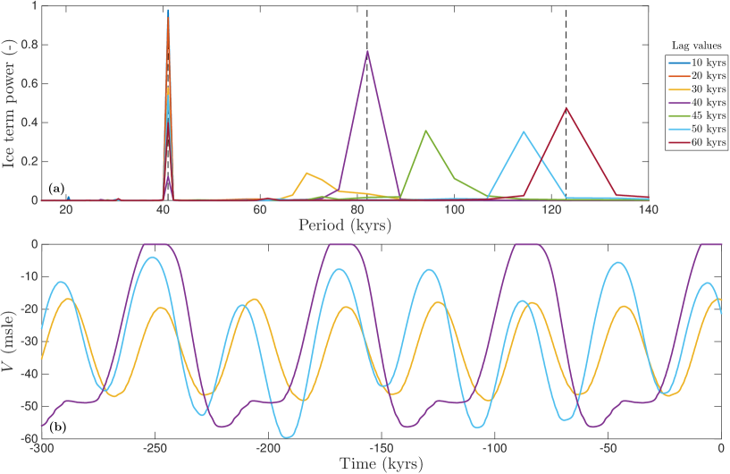
Figure 9: Model for different MOR lag times. Results use obliquity-only insolation, with $\gamma_{\textrm{MOR}}$ non-zero and $\gamma_{\textrm{T}},\gamma_{\textrm{SAV}}=0$. Panel (a) shows the strength of DFT terms for the ice volume timeseries. The power spectra terms sum to unity. Panel (b) shows select ice volume timeseries over the final 300 kyrs of the model run. The dotted lines mark the 41 kyr obliquity period and its multiples. The mantle permeability range represented by the MOR lag values is $10^{-11}$–$10^{-8.5}$ m² at 1% porosity.

We highlight two features of these results: firstly, they show that lag times $<20$ kyr do not influence the periodicity of glacial cycles. This implies that $C$ feedbacks operating at less than the $<20$ kyr timescale (hereafter, short-timescale) do not affect the periodicity of glacial cycles.

We term these short-timescale feedbacks because they are shorter than the obliquity period (i.e., the default glacial cycle period). This is an important distinction, short-timescale feedbacks act on an intra-cycle basis, modulating the magnitude of glacial cycles and — in tandem with insolation — controlling the timing of peak climates (see the offset of different coloured sine peaks in figure 9b). However, the short-timescale feedbacks carry little information from one glacial cycle to the next and are therefore ineffective at disrupting obliquity-linked 40 kyr cycles.

Thus, short-timescale $C$ feedbacks only affect the magnitude of ice and temperature changes during glacial cycles; this is true for both negative $C$ feedbacks (i.e., acts to oppose sea-level change) shown in this section and positive $C$ feedbacks (see figures 13 and 14). Consequently, the model’s glacial cycles are sensitive to the net $C$ change caused by short-timescale $C$ feedbacks, but relatively insensitive to how the $C$ change is distributed on very short timescales. This helps justify our lumping surface system carbon feedbacks into a single parameter, and suggests we can be agnostic about how carbon feedbacks are distributed over short timescales if the net carbon change is correct (i.e., our model can have inaccurate $\gamma_{\textrm{T}}$ and $\gamma_{\textrm{SAV}}$, provided that their collective effect on $C$ is accurate). This reduces concerns about the uncertainty of the amplitude of SAV’s $\text{CO}_{2}$ response to glacial cycles.

Secondly, these results largely support the concept that 30–50 kyr lags can disrupt 40 kyr glacial cycles. A smaller range of $\simeq$$40$ kyr lag times generate sustained glacial cycles with 80 kyr periods and $\simeq$$60$ kyr lag times generate glacial cycles with 120 kyr periods. Of these lag times, the $40$ kyr MOR lag causes the most power in the $\sim$100 kyr period band, and thus is the optimal lag for introducing $\sim$100 kyr glacial cycles into an obliquity-dominated Earth system. To streamline results and discussion, we use this optimal $40$ kyr lag time in subsequent sections. However, under real orbital forcing with power across a range of frequencies we expect a small range of lags to be similarly effective at disrupting 40 kyr cycles, because exact (anti-)resonance with 40 kyr orbital cycles will be a relatively less important effect.

These results provide us with the optimal MOR lag time for creating $\sim$100 kyr glacial cycles, and demonstrate that our model system has no inherent 100 kyr periodicity until MOR $\text{CO}_{2}$ responses are introduced as an intercycle feedback. With the MOR lag time chosen, we now consider the effects of varying the strength of terms in our $\text{CO}_{2}$ feedback equation (8).

4.2 Full model behaviour

In this section all terms in our $\text{CO}_{2}$ model (eqn (8)) are active; atmospheric $\text{CO}_{2}$ concentration, $C$, varies according to our parameterised surface system and volcanic effects. Insolation forcing includes obliquity, precession, and eccentricity. We refer to this as the ‘full model’ configuration. We explore model behaviour by varying all three sensitivity parameters in the $\text{CO}_{2}$ equation (appendix A.7 shows the model with only single carbon terms active). We first observe behaviour with timeseries plots, then use Fourier transforms of ice volume, $V$, to highlight the changing periodicity of ice volume as $C$ feedback parameters are changed. Our benchmark for $\sim$100 kyr cycles is figure 7c — the $V$ timeseries calculated by our model when forced by both an imposed, ice-core $\text{CO}_{2}$ timeseries and insolation. We compare our DFT terms from the full model to this ‘ice core replication’ benchmark to determine if the model is producing $\sim$100 kyr cycles.

Figure 10 shows how the full model varies with increasing $\gamma_{\textrm{MOR}}$. For $\gamma_{\textrm{MOR}}=14$ Mt$\text{CO}_{2}$/yr per cm/yr the model has reasonable amplitude $C$ cycles ($\sim$80 ppmv) and generates $V$ cycles with significant 100 kyr periodicity. Thus the amplitude of $C$ cycles are reasonably close to late-Pleistocene values when the ‘full model’ is close to replicating the ice core $\sim$100 kyr glacial cycles (this trend holds across sensitivity factor values). Increasing $\gamma_{\textrm{MOR}}$ increases the magnitude of $C$ cycles and adds greater 100 kyr variability. We now consider the periodicity of these model runs across a parameter sweep in the model’s three sensitivity factors $\gamma_{\textrm{T}}$, $\gamma_{\textrm{SAV}}$, and $\gamma_{\textrm{MOR}}$.

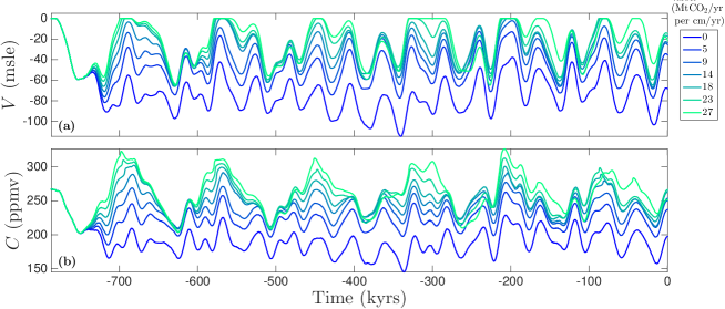
Figure 10: Increasing the sensitivity of MOR $\text{CO}_{2}$ emissions to sea level $\gamma_{\textrm{MOR}}$, with $\gamma_{\textrm{T}}=10$ ppmv/K, $\gamma_{\textrm{SAV}}=18$ Mt$\text{CO}_{2}$/yr per cm/yr change in sea level. Panel (a) is ice volume in metres sea level equivalent. Panel (b) is $\text{CO}_{2}$ concentration in the atmosphere. The change dominant period occurs in both $V$ and $C$ as $\gamma_{\textrm{MOR}}$ is increased, and occurs for the full time of the model run.

As mentioned above, we quantify the magnitude of the $40$ kyr and $\sim$100 kyr periodicities in ice volume by comparing them to the same periodicities (over the same time interval) in the model ice core replication shown in figure 7c. Specifically, we apply a discrete Fourier transform to each of these $V$ timeseries and sum the terms in the frequency bands corresponding to 40 kyr and 80–120 kyr periodicity, then divide the ‘full model’ value by the ice core replication value — if the result is above $1$ then there is more power present (in that frequency band) in the full model than there was in the calculated ice volume for Late Pleistocene conditions. This parity criterion is marked with a red contour line in figure 11. For $\sim$100 kyr cycles the minimum MOR emissions sensitivity to meet this parity criterion is $\gamma_{\textrm{MOR}}=11$ Mt$\text{CO}_{2}$/yr per cm/yr.

Figure 11 shows 40 kyr periodicity decreasing in strength for increasing $\gamma_{\textrm{MOR}}{}$, whilst the $\sim$100 kyr periods increase in strength. This matches the predictions in prior sections and the behaviour in figure 10; MOR $\text{CO}_{2}$ emissions with a lag of $40$ kyrs oppose every second obliquity cycle and create a stable feedback with an 80–120 kyr glacial cycle.

The trends in $\gamma_{\textrm{MOR}}$ values that cause the full model to reach and exceed the parity criterion for $\sim$100 kyr $V$ cycles is as predicted in prior sections. Recall that MOR $\text{CO}_{2}$ emissions variations are directly proportional to the magnitude of sea-level change, and positive short-timescale intra-cycle feedbacks like $\gamma_{\textrm{T}}$ and $\gamma_{\textrm{SAV}}$ increase sea-level change. Therefore, the required $\gamma_{\textrm{MOR}}$ value to match the parity criterion decreases as $\gamma_{\textrm{T}}$ or $\gamma_{\textrm{SAV}}$ increase. When trading off between $\gamma_{\textrm{T}}$ and $\gamma_{\textrm{SAV}}$, a lower $\gamma_{\textrm{SAV}}$ gives a lower minimum $\gamma_{\textrm{MOR}}$ to reach parity for $\sim$100 kyr cycles, shown by the top-right panel in figure 11 having the red parity contour reach lower $\gamma_{\textrm{MOR}}$ values than in the lower-right panel.

For very high $\gamma_{\textrm{T}}$ or $\gamma_{\textrm{SAV}}$, the $V$ cycle amplitude increases. Runaway positive feedbacks in this limit (from larger ice sheets and decreasing temperatures) lead to a permanent glaciation, akin to a ‘Snowball Earth’. It is not clear if such runaway scenarios are reasonable representations of a marginal stability in the Earth system, or a model failure (i.e., parameterized feedbacks and forcings becoming inaccurate in very cold, low $\text{CO}_{2}$ conditions that have no parallel in the Pleistocene record). The largest stable $\gamma_{\textrm{T}}$ values give model runs with sea-level changes of 85–100 metres, so our full model captures glacial cycles with physical conditions similar to historical glacial cycles. Therefore we do not believe we are missing parameter space relevant to the Pleistocene.

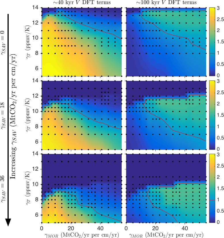
Figure 11: Periodicity of model runs for the last 787 kyrs with $\gamma_{\textrm{SAV}}=0,18,36$  Mt$\text{CO}_{2}$/yr per cm/yr change in sea level for the three rows. Plots show the strength of terms in the discrete Fourier transform of ice volume relative to the model output in figure 7(a). The left plots show 40 kyr terms, the right plots 80–120 kyr terms. The red contour marks where the full model matches our modelled glacial replication. Dark blue marks where the model enters a runaway glacial event, we chose not to plot these as FFTs are not valid for timeseries that have a sharp change in periodicity partway through.

The power spectra for the full model at parity (i.e., near the red contour in figure 11) have power in the 23/41/100 kyr bands of 3%, 35%, and 50% respectively. Compared to our figure 7 ice core replication (5.6%, 23%, 50%), or sea-level data (4%, 10%, 55%) the full model is underpowered in the precessional band, and overpowered in the obliquity band. Despite this, the full model spectra (at parity) are a reasonable match for glacial cycles.

Overall, the full model system can switch from 40 kyr glacial cycles to $\sim$100 kyr cycles, the calculated $\sim$100 kyr cycles are stable (figure 10), and the minimum required sensitivity of MOR $\text{CO}_{2}$ emissions to sea level is $\gamma_{\textrm{MOR}}=11$ Mt$\text{CO}_{2}$/yr per cm/yr change in sea level (figure 11). This $\gamma_{\textrm{MOR}}$ requires MOR $\text{CO}_{2}$ emissions at the upper end of a 95% confidence interval (see section 5) according to most prior work, thus this $\gamma_{\textrm{MOR}}$ value is possible, but not likely.

5 Discussion

We have presented a simplified model of climate through glacial–interglacial cycles. The model comprises three variables — temperature, ice sheet volume, and $\text{CO}_{2}$ concentration in the atmosphere — these evolve according to equations based on the physics of insolation, heat transfer in the atmosphere and Earth’s surface, radiative $\text{CO}_{2}$ forcing, ice flow under stress, proposed MOR $\text{CO}_{2}$ emissions processes, and parameterizations of the surface carbon system, subaerial volcanic $\text{CO}_{2}$ emissions, and water vapour plus cloud forcing. The model calculates glacial-interglacial behaviour with insolation as the sole driver of the system and $\text{CO}_{2}$ concentration in the atmosphere as an internal feedback. Although the model captures important and fundamental physics, it neglects many processes that may affect the results, which we discuss below.

We treat the atmosphere as a single layer and parameterise the net upward and downward longwave greenhouse effects. The parameterisation gives the overall energy balance between space, atmosphere, and ground but ignores changes in the internal atmospheric temperature structure. It is possible that important features are missed in this simplification, but our model does calculate reasonable present-day temperature distributions, seasonality (figure 3), $\text{CO}_{2}$-doubling scenarios (figure 4), and glacial replications (figure 7).

The ice model assumes a flat topography, distorted only by isostasy, and assumes no longitudinal variations in ice. Flat, low-lying topography suppresses initial ice formation and ignores the complexity of advancing ice sheets across the terrain of North America and Europe, but figure 7 shows our model replicating reconstructed sea-level timeseries, suggesting that the simplification is reasonable nonetheless. The computational complexity of the global 3D temperature and ice models required to relax these simplifying assumptions are too computationally expensive for Ma-scale studies; previous work on glacial ice sheets made similar simplifications (Tarasov and Peltier, 1997; Fowler et al., 2013).

We do not explicitly include oceans in our model, they are implicitly incorporated into the temperature-dependent surface system term in equation (8) . However, oceanic effects (that we have neglected) should reduce volcanism-driven $C$ variations — extra absorbtion/venting of $\text{CO}_{2}$ to/from oceans when the atmospheric $\text{CO}_{2}$ concentration is out of equilibrium with the surface ocean. These are significant shortcomings, however there are no published ocean models that allow us to explicitly model oceanic $\text{CO}_{2}$ effects by dynamically replicating glacial-to-interglacial oceanic transitions. We believe the clear simplifications we make are better than building an ad-hoc ocean model. It would be an improvement to the current work if the qualitative ideas of glacial oceanic changes (iron fertilisation of the South Atlantic, shifting latitudes of southern ocean westerlies, changing relative deepwater formation rates in the North Atlantic vs. Antarctica, etc…) were included in an ocean model that makes quantitative changes to atmospheric $\text{CO}_{2}$ concentration.

We consider volcanic $\text{CO}_{2}$ emissions in our modelling, yet other glacially-driven volcanic changes could affect climate, such as SAV aerosols, MOR hydrothermal flux, and Fe flux. It is not clear if including these extra volcanic effects in a model would affect the switch to $\sim$100 kyr glacial cycles. If future research reveals any to have large climate feedbacks on 10’s-of-kyr timescales, that would impact the conclusions of this work.

Our model is a deterministic system and, unlike geological records of glacial cycles, has no noise on (e.g.,) $<$200 year timescales. However, noise does not effect our model’s conclusions. When we introduce noise in input parameters, we see no change in qualitative model behaviour (appendix A.8).

Even after accounting for simplifications, our model gives insight into glacial–interglacial behaviour. Previous work takes dependent variables in the earth system (temperature, atmospheric $\text{CO}_{2}$ concentration, ice extent) and uses them as independent driving variables — clearly shortcomings when considering the highly coupled glacial system whose key features emerge on the 10s-of-kyrs timescale. This model addresses those features, with space for uncertainties to be reduced or further mechanisms explored.

We see a sharp distinction between climate feedbacks acting at significantly less than the glacial period (short-timescale feedbacks) and those acting at or above the glacial timescale. Short-timescale $C$ feedbacks are intracycle effects that modulate the magnitude of each glacial, but because they carry little information from one glacial cycle to the next, are ineffective at changing overall glacial periodicity.

Our model finds transitions from $40$ kyr cycles to $\sim$100 kyr cycles as we increase MOR $\text{CO}_{2}$ emissions response to rate-of-sea-level-change (i.e., increasing $\gamma_{\textrm{MOR}}$). There is no significant 100 kyr variability without the intercycle feedback from MORs. The transition mechanism is atmospheric $\text{CO}_{2}$ concentration (influenced by MOR $\text{CO}_{2}$ emissions) acting to suppress a glacial–interglacial transition triggered by insolation. The subsequent increase in sea-level periodicity from $40$ kyrs to $80$–$120$ kyrs approximately doubles the magnitude of MOR $\text{CO}_{2}$ variability (fig 6), and short-timescale $C$ feedbacks reinforce the new cycle and produce large $C$ changes that dominate insolation such that only every second or third obliquity cycle causes major deglaciation.

This transition mechanism inherently generates sawtooth patterns in $V$ (fig 9b), describing a growing ice sheet, interrupted growth (when $C$ and insolation are in opposition), followed by further growth, and then a large deglaciation.

Our model’s transition to $80$–$120$ kyr glacial cycles is broadly consistent with the coupled oscillator model of Huybers and Langmuir (2017), suggesting analagous behaviour may govern our system.

Under optimal conditions the model transitions to $\sim$100 kyr cycles at $\gamma_{\textrm{MOR}}=11$ Mt$\text{CO}_{2}$/yr per cm/yr change in sea level. Physically this corresponds to MOR emissions of 91 Mt$\text{CO}_{2}$/yr changing up to $\pm 12\%$ across a glacial cycle, or (recalling that our $\gamma_{\textrm{MOR}}$ is linear in baseline emissions and percentage change) a scaled equivalent e.g., 137 Mt$\text{CO}_{2}$/yr changing up to $\pm 8\%$. Are these volcanic numbers feasible? For our specified MOR lag time, models predict $\gamma_{\textrm{MOR}}=8\%$ (Burley and Katz, 2015) with little room for error (uncertainties in the model inputs would not change predicted $\gamma_{\textrm{MOR}}$ by $\pm 1$ percentage point), thus we must ask if 137 Mt$\text{CO}_{2}$/yr is a reasonable background global volcanic $\text{CO}_{2}$ emissions rate.

It is worth considering global MOR $\text{CO}_{2}$ emissions in some detail, given the diverse literature. There are two approaches to estimating global MOR $\text{CO}_{2}$ flux, all based around measuring an element that has a constant ratio to $\text{CO}_{2}$ in volcanic eruptions, then using that fact (plus other assumptions) to calculate $\text{CO}_{2}$ emissions: 1) use the concentration of ³He in ocean water to infer the rate of MOR $\text{CO}_{2}$ emissions. The element must have a known lifetime in the ocean (preferably with no non-volcanic inputs). 2) use the concentration of an element in volcanic rocks to infer the $\text{CO}_{2}$ concentration in the source mantle. Then apply a melting fraction to generate an erupting mantle composition from the source mantle, and multiply by the volume of mantle erupted per year to calculate the rate of MOR $\text{CO}_{2}$ emissions. The first approach has a single method, ³He in the oceans, which has settled to values of 0–134 Mt$\text{CO}_{2}$/yr (Resing et al., 2004) and $18$–$176$ Mt$\text{CO}_{2}$/yr (Marty and Tolstikhin, 1998) (2 std.dev.). Updated ³He flux values from Bianchi et al. (2010) would change these values to 0–101, and 9–93 Mt$\text{CO}_{2}$/yr respectively. For the second approach, the most recent work combining ratios of Nb, Rb and Ba for melt inclusions calculates $18$–$141$ Mt$\text{CO}_{2}$/yr (2 std.dev.) (Le Voyer et al., 2017). Work using the undegassed Siqueiros melt inclusions calculates $29$–$53$ Mt$\text{CO}_{2}$/yr (2 std.dev.) (Saal et al., 2002) (the Siqueiros melt inclusions may be highly depleted, implying their derived global emissions value is an underestimate) and volcanic glasses give $88$–$158$ Mt$\text{CO}_{2}$/yr (2 std.dev.) (Michael and Graham, 2015). There could be systematic error in some of these measurements, particularly given the sensitivity of the latter approaches to the assumed average mantle melt fraction used to generate MOR basalts (i.e., erupting mantle composition) from the MOR mantle source (Cartigny et al., 2008; Dasgupta and Hirschmann, 2010; Le Voyer et al., 2017). Furthermore, none of these studies include uncertainty in the degree of melting in their random error, so errors are likely underestimated. Using the latest melting models, Keller et al. (2017) calculate a range of 53–110 Mt$\text{CO}_{2}$/yr for $\text{CO}_{2}$ concentration in the MOR mantle source is 100–200 ppmw. Extrapolating linearly (a vast simplification) to a 2-$\sigma$ range in $\text{CO}_{2}$ concentration of 27–247 ppmw (Le Voyer et al., 2017) gives 14–135 Mt$\text{CO}_{2}$/yr. Our required emissions of 137 Mt$\text{CO}_{2}$/yr is at the high end of the 95% confidence interval for some of these studies, therefore it is possible, although not likely, that the global MOR $\text{CO}_{2}$ emissions rate is large enough to disrupt glacial cycles, assuming no oceanic moderation of volcanic emissions.

However, if we assume volcanic $\text{CO}_{2}$ variability’s effect on $C$ is damped by oceanic absorption/emission, then the required MOR parameters are outside the expected range. This ‘oceanic damping’ logic is based on the idea that the surface ocean and atmospheric $\text{CO}_{2}$ are in equilibrium, and that any attempt to change the atmospheric $\text{CO}_{2}$ concentration is opposed by changes in ocean chemistry. Such logic represents anthropogenic carbon changes well, but glacial cycles probably involve changes in the physical ventilation of the oceans, making the comparison inexact; modern models are a worst case scenario. Regardless, modern Earth system models (Archer et al., 2009) suggest a factor of 4 increase in required background MOR emissions — necessitating 548 Mt$\text{CO}_{2}$/yr, outside the upper limits of MOR $\text{CO}_{2}$ emissions. Even a factor of 1.5 increase would require unreasonable MOR $\text{CO}_{2}$ emissions. Therefore despite the uncertainty in oceanic $\text{CO}_{2}$-damping effects, background MOR $\text{CO}_{2}$ emissions are very unlikely to meet the requirements for $\sim$100 kyr cycles after accounting for ocean absorption.

The magnitude of changes in MOR and SAV $\text{CO}_{2}$ emissions are proportional to the magnitude of sea-level change, and MOR $\text{CO}_{2}$ emissions increase for longer period sea level changes. Therefore, if MOR $\text{CO}_{2}$ emissions are part of the transition mechanism from $40$ to $100$ kyr glacial cycles, the model suggests the following: 1) transitioning to $\sim$100 kyr glacial cycles will increase the magnitude of $\text{CO}_{2}$, sea-level, and temperature changes — including warmer interglacial periods, and 2) a relatively large sea level change should precede the transition to longer glacial cycles.

This process of volcanic $\text{CO}_{2}$ emissions altering glacial cycles is consistent with the results of Tzedakis, P. C. . et al. (2017), where the summer insolation required to trigger full deglaciation increases across -1.5 Ma to -0.6 Ma (after accounting for discount rate, whereby deglaciation has a lower insolation threshold the longer an ice sheet has existed). Their discount rate is conceptually consistent with ice sheet instability as explained in Clark and Pollard (1998); Abe-Ouchi et al. (2013), however the changing insolation threshold is not readily explained by existing theories. A plausible explanation is a feedback cycle whereby an increase in the magnitude of sea-level changes leads to increased volcanic $\text{CO}_{2}$ emissions variability — amplifying $\text{CO}_{2}$ (and thus temperature) variations — consequently amplifying the next sea-level cycle. This eventually changes the period of sea-level cycles as MOR $\text{CO}_{2}$ emissions variability becomes larger; leading to further increases in MOR $\text{CO}_{2}$ emissions (section 3.1) and even larger sea-level cycles, until the system reaches a new steady state with large, long period sea-level cycles. The feedback between volcanism and sea-level would take several glacial cycles to reach a new equilibrium, consistent with the 900 kyr transition time proposed in Tzedakis, P. C. . et al. (2017).

6 Conclusion

We have presented a reduced-complexity model system that calculates the Earth climate over the past 800 kyrs; a system with ice sheets, $\text{CO}_{2}$ concentration in the atmosphere and other forcings evolving in response to imposed insolation changes. We demonstrated a match to current planetary temperatures and GCM $\text{CO}_{2}$ doubling forecasts. When driven with observed $\text{CO}_{2}$, the model reproduces the glacial sea-level record.

Our main research interest was quantifying the mid-ocean ridge (MOR) $\text{CO}_{2}$ emissions sensitivity to sea-level change necessary to induce $\sim$100 kyr glacial cycles, thus assessing the plausibility of volcanic mechanisms for creating an Earth system climate response not linearly related to insolation forcing.

Our model has no intrinsic 100 kyr variability until the lagged response of MOR’s $\text{CO}_{2}$ emissions to sea level change is included; default behaviour is 40 kyr glacial cycles. We calculate that MOR $\text{CO}_{2}$ variability, above a threshold sensitivity to sea-level change, causes glacial cycles at a multiple of insolation’s 40 kyr obliquity cycle. These $\sim$100 kyr cycles are asymmetric, and occur at both 80 kyr and 120 kyr periods, replicating features of the late-Pleistocene glacial record.

However, even under optimal conditions, $\sim$100 kyr cycles require MORs’ $\text{CO}_{2}$ emissions response be $11$ Mt$\text{CO}_{2}$/yr per cm/yr rate of sea-level change, 50$\%$ higher than the expected $7.3$ Mt$\text{CO}_{2}$/yr per cm/yr. This requires background MOR $\text{CO}_{2}$ emissions of 137 Mt$\text{CO}_{2}$/yr, within the 95% confidence interval of (some) estimates of MOR $\text{CO}_{2}$ flux. However, under less optimal conditions where oceanic effects moderate MOR emissions’ effect on $C$, required baseline MOR $\text{CO}_{2}$ emissions are over 200 Mt$\text{CO}_{2}$ per year — highly improbable. This suggests that MOR $\text{CO}_{2}$ emissions are not, in isolation, responsible for glacial cycles $>40$ kyrs.

Of course, MOR $\text{CO}_{2}$ emissions do not act in isolation, and there are relevant glacial mechanisms that do not operate in our model, including regolith erosion(Clark and Pollard, 1998), secular $\text{CO}_{2}$ decline (Pagani et al., 2010; Hönisch et al., 2009), and switching modes in ocean ventilation (Franois et al., 1997; Toggweiler, 1999). These mechanisms may interact with our existing processes to allow glacial cycles at lower MOR $\text{CO}_{2}$ variability. However, adding such mechanisms would increase model complexity; furthermore, these mechanisms are not precisely defined and would necessitate a wide range of representative models and parameter sweeps. Thus it is unlikely that a mixed mechanism hypothesis for $\sim$100 kyr glacial cycles can be tested until each mechanism is more precisely defined.

Our model system highlights other important features. First, we calculate that the net changes in atmospheric $\text{CO}_{2}$ concentration caused by MOR volcanism will approximately double when sea-level periods increase from 40 kyrs to 100 kyrs. Therefore, if a $\sim$100 kyr glacial cycle occurs, MOR volcanism acts to reinforce that periodicity.

Second, our model makes a distinction between intracycle and intercycle feedbacks. An intracycle feedback is a process with a timescale less than half the glacial cycle period; therefore acting within a glacial cycle. Intracycle feedbacks affect the magnitude of glacial cycles, but cannot change the glacial periodicity. This result will hold for any feedback process with constant sensitivity.

Third, we found that MOR systems with a 40 kyr lag between sea-level change and consequent $\text{CO}_{2}$ emissions generate $100$ kyr cycles at the lowest $\gamma_{\textrm{MOR}}$. However, any intercycle feedback in the Earth system can potentially generate $\sim$100 kyr cycles, and we calculate significant power at $\sim$100 kyr for MOR lags of 30–80 kyrs. Therefore the proposed volcanic mechanism for 100 kyr glacial cycles is not dependent on a peculiarly specific MOR lag value (equivalently, a particular mantle permeability).

Finally, without strong MOR $\text{CO}_{2}$ emissions sensitivity, our model defaults to an obliquity-linked glacial cycle with a $40$ kyr period; precession’s $23$ kyr cycle has little effect on the ice sheet. This result is in agreement with previous work considering integrated summer forcing, and is the first time that $40$ kyr response has been shown dominant in a model with radiative feedbacks. Therefore our model opposes the hypothesis that precession-linked glacial cycles may have occurred before the mid-Pleistocene transition, with anti-phase changes in Antarctic and Greenland ice mass at the $23$ kyr period leaving a predominant 41 kyr signal in the $\delta^{18}\textrm{O}$ record (Raymo et al., 2006).

The model’s conclusion could be sensitive to some of our simplifications, such as the oceans’ interaction with volcanic emissions on glacial timescales and the climate effect of other variable volcanic elements. However, these effects are all beyond current understanding and it is hard to predict their effect on our model. Complete understanding of glacial cycle dynamics will require models including several of the mechanisms currently proposed in literature. We hope that future work can build on the base that we have presented.

Acknowledgements

The research leading to these results has received funding from the European Research Council under the European Union’s Seventh Framework Programme (FP7/2007-2013) / ERC grant agreement number 279925. The University of Oxford Advanced Research Computing (ARC) facility was used in this work (doi:10.5281/zenodo.22558). Katz thanks the Leverhulme Trust for additional support. We thank D. Battisti and J. Moore for helpful discussions.

Appendix A Appendix

A.1 EBM Model

The EBM is constructed around energy balance equations for the middle atmosphere (4), ground surface (5), and subsurface (6), repeated below:

$$c_{a}\dfrac{\partial{T_{a}}}{\partial{t}}=S_{a}+I_{a}+F_{s}+D_{a}\;\;,$$ (9)

$$c_{s}\dfrac{\partial{T_{s}}}{\partial{t}}=S_{s}+I_{s}-F_{s}+F_{ss}\;\;,$$ (10)

$$c_{ss}\dfrac{\partial{T_{ss}}}{\partial{t}}=-F_{ss}\;\;,$$ (11)

where $a,s,ss$ subscripts define atmospheric, surface and subsurface quantities. $c$ is heat capacity (Jm^-2K^-1), $S$ is the solar radiation (shortwave), $I$ is infrared longwave radiation, $F$ is the sensible heat flux, and $D_{a}$ is the meridional heat flux. All the RHS quantities are Wm^-2 and are detailed below.

Solar radiation is treated as reflecting between the ground and a single atmospheric layer. The atmosphere has reflectivity $R$, absorption $A$, and transmissivity $T$ — these sum to 1. The ground has reflectivity (equivalently, albedo) $\alpha$, which has two values representing ice/non-ice conditions. Thus

$$S_{a}=AS+\frac{TAS\alpha}{1-\alpha R}\;\;,$$ (12)

$$S_{s}=TS\frac{1-\alpha}{1-\alpha R}\;\;,$$ (13)

where the ground-atmosphere reflections are included as the sum of a geometric series. The model atmosphere has a single values for shortwave reflectivity and transmissivity, whereas real atmospheric reflectivity should vary with latitude due to increased cloud cover at high latitudes (Donohoe et al., 2011). Higher reflectivity at high latitude would 1) make variable insolation a weaker driver of glacial cycles, and 2) reduce the albedo effect of ice sheets, which are stronger in our model than in GCMs.

The infrared components are treated as imperfect black body radiators, giving

$$I_{s}=\epsilon_{a}\sigma T^{4}_{as}-\sigma T^{4}_{s}\;\;,$$ (14)

$$I_{a}=\sigma T^{4}_{s}-\epsilon_{a}\sigma T^{4}_{as}-\epsilon_{a}\sigma T^{4}_{ul}\;\;,$$ (15)

where $\epsilon_{a}$ is the longwave atmospheric emissivity, $\sigma$ is the Stefan-Boltzmann constant, $T_{as}$ is the atmospheric temperature at the ground surface and $T_{ul}$ at upper atmosphere. The atmospheric temperatures are related to the middle atmosphere temperature by a constant moist adiabatic lapse rate $\Gamma_{m}$ of $6.5~{}$K/km. The alternative of a spatially and temporally varying lapse rate requires assumptions about the global hydrological cycle that we choose to circumvent. Applying the lapse rate to the previous equations gives

$$I_{s}=\epsilon_{a}\sigma T^{4}_{as}-\sigma(T_{a}+\Gamma_{m}H_{as})^{4}\;\;,$$ (16)

$$I_{a}=\sigma T^{4}_{s}-\epsilon_{a}\sigma(T_{a}+\Gamma_{m}H_{as})^{4}-\epsilon_{a}\sigma(T_{a}+\Gamma_{m}H_{ul})^{4}\;\;,$$ (17)

where $H_{ul}$ is the distance from the middle atmosphere to the upper atmosphere, $H_{as}$ is the distance from the middle atmosphere to the ground surface, which varies with thickening ice sheets and bed depression. The upper atmosphere is defined as the height the atmosphere becomes optically thin to IR radiation and varies with $C$ to represent radiative $\text{CO}_{2}$ forcing (see section A.3).

Sensible heat flux scales linearly with the temperature difference between adjacent surfaces:

$$F_{ss}=K_{s}\left(T_{ss}-T_{s}\right)\;\;,$$ (18)

$$F_{s}=K_{ss}\left(T_{s}-(T_{a}+\Gamma_{m}H_{as})\right)\;\;,$$ (19)

where $K$ is the coefficient parameterising the heat flux.

The meridional heat transport scales with the meridional heat gradient,

$$D_{a}=\dfrac{\partial{}}{\partial{\phi}}\left(-K_{a}\left|\dfrac{\partial{T_{a}}}{\partial{\phi}}\right|\dfrac{\partial{T_{a}}}{\partial{\phi}}\right)\;\;,$$ (20)

and this transport is tuned to a reasonable value by selecting $K_{a}$. We follow the $1000$ J/K per degree latitude used in Huybers and Tziperman (2008).

To get to the energy available for melting ice the energy balance model is run for a year, with 1-day explicit timesteps to account for seasonality. At each timestep, the energy flux in/out of the ground surface is calculated; this energy flux changes the surface temperature or melts ice according to the local conditions. The thickness of ice melted is then calculated assuming constant ice density on the ice sheet’s upper surface.

Finally, the model needs precipitation to accumulate ice. Precipitation is dependent on temperature as described in eqn (24). At each timestep, wherever the atmospheric temperature at the ground surface is below freezing, this precipitation falls as snow and creates an ice sheet. Where atmosphere is above freezing, the precipitation has no effect on the ice thickness or energy balance.

Variable	Value		Description
$\alpha_{g}$	$0.3$		land albedo
$\alpha_{i}$	$0.8$		ice albedo
$\Gamma_{m}$	$6.5$	K/km	moist adiabatic lapse rate
$\epsilon_{a}$	$0.85$		longwave atmospheric emissivity
$\rho_{l}$	$900$	kg/m3	ice density
$\rho_{w}{}$	$1000$	kg/m3	water density
$\rho_{a}$	$1.5$	kg/m3	surface air density
$\sigma{}$	$5.67\times 10^{-8}$	W/(m2K4)	Stefan-Boltzmann constant
$C_{p}$	$2100$	J/(kg K)	specific heat capacity of water
$C_{air}$	$1.5$	J/(kg K)	specific heat capacity of air
$C_{a}$	$5000\rho_{a}C_{air}$	J/(m2K)	atmospheric heat capacity
$C_{s}$	$5\rho_{i}C_{p}$	J/(m2K)	surface heat capacity
$C_{ss}$	$10\rho_{i}C_{p}$	J/(m2K)	subsurface heat capacity
$g$	$9.8$	m/s2	gravitational acceleration
$H_{as}$	$5$	km	height of middle atmosphere above sea-level
$H_{ul}$	$2$	km	upper atmosphere thickness
$K_{s}$	$5$	W/(m2 K)	Thermal transmittance, surface–atmosphere,
			the sensible heat flux coefficient
$K_{ss}$	$2$	W/(m2 K)	Thermal transmittance, surface–subsurface
$K_{a}$	$1000/(^{o}$ lat)	J/K	meridional heat flux coefficient
$L_{v}$	$2.5\times 10^{6}$	J/kg	latent heat of vaporization
$L_{m}$	$3.34\times 10^{6}$	J/kg	latent heat of melting
$L_{s}$	$2.84\times 10^{6}$	J/kg	latent heat of sublimation
$S$	$1365$	W/m2	solar constant
$A$	$0.2$		absorption of atmosphere
$R$	$0.3$		reflection of atmosphere
$T$	$0.5$		transmission of atmosphere

Table 2: Parameters used for the EBM.

A.2 EBM Modifications

We make two major changes to the EBM scheme of Huybers and Tziperman (2008): adding longwave radiative forcings based on atmospheric composition, and creating a variable precipitation based on local temperature. These are explained below.

First we discuss our longwave radiative modifications; adding forcings representing $\text{CO}_{2}$, water vapour, lapse rate, and cloud effects. These radiative forcings are treated with two terms: one for the $\text{CO}_{2}$ forcing, and another for the aggregate effects of water vapour, lapse rate and cloud forcings. We add these forcings to a single-layer atmosphere that has an imposed linear temperature profile $\textrm{d}T/\textrm{d}z$ of $6.5$ K/km. The base of the atmosphere is at the ground surface (land or the top of an ice sheet). The upper surface of the atmosphere is the mean height at which the atmosphere becomes transparent to longwave radiation and allows longwave emissions to to escape to space. In the model’s neutral state, this is 6.5 km above sea level, well within the troposphere’s linear temperature profile. Therefore, changes in the height of the mean emissions layer will change its temperature; this changes the power of longwave emissions to space according to the Stefan-Boltzmann law.

Greenhouse gas forcing occurs because such gases alter the height at which atmosphere becomes transparent to longwave radiation. Our model scheme is guided by this physics; implementing top-of-atmosphere forcing by altering the height of the emissions layer.

The upward longwave (ULW) radiative $\text{CO}_{2}$ forcing is derived from Myhre et al. (1998) global mean forcing,

$$\bar{R}_{\textrm{ULW}}=\lambda\log_{2}\left(\frac{C}{C_{0}}\right)\;\;,$$ (21)

where $\bar{R}_{\textrm{ULW}}$ is the global average radiative forcing (we use $R$ instead of typical forcing terminology ‘$F$’ to avoid confusion with the EBM’s heat flux terms), $\lambda$ is $\text{CO}_{2}$ sensitivity in W/m² per $\text{CO}_{2}$-doubling, and $C_{0}=280$ ppmv is the reference concentration of $\text{CO}_{2}$ in the atmosphere. We follow the conclusions of Stap et al. (2014) and Köhler et al. (2010) for greenhouse forcing in the Pleistocene and assume a $30$% increase in $\text{CO}_{2}$ forcing magnitude from syncronous increases other greenhouse gases. Thus $\lambda$ is $4.85$ W/m² per $\text{CO}_{2}$-doubling.

We convert this global average forcing to a latitude-dependent forcing ${R}_{\textrm{ULW}}$ by changing the height (and therefore temperature) of the atmospheric layer emitting longwave radiation to space — details are given in appendix A.3. A reasonable summary is to consider a global temperature change of the emitting layer $\Delta T$ (assumes $\textrm{d}T/\textrm{d}z$ independent of $\phi$), changing Stefan-Boltzmann emissions by $(T_{ul}+\Delta T)^{4}-T_{ul}^{4}$. Upper atmosphere temperature $T_{ul}$ varies with $\phi$, and the forcing is thus latitude-dependent. This forcing is applied to the net infrared energy balance of the atmosphere in equation 23 below.

DLW is parameterized to match the calculations in Cai and Tung (2012) of longwave $\text{CO}_{2}$ forcing at the bottom of the atmosphere in a 2D GCM. Our parameterised equation is a logistic function and an exponential

$$R_{\textrm{DLW}}=K\left(\frac{1}{1+e^{(a-\phi)/b}}+\frac{e^{(-\phi/c)}}{3}\right)\;\;,$$ (22)

where $K$ is the maximum forcing, $a=30^{\textrm{o}}$ is the latitude of the logistic function turning point, $b$ scales the width of the logistic function’s growth region and $c$ scales the e-fold length of the decreasing exponential. For a given $\text{CO}_{2}$ concentration, $K$ is equal to the maximum value of ${R}_{\textrm{ULW}}$.

We model the combined global energy balance effects of water vapour, lapse rate and clouds as a radiative longwave forcing, varying linearly with changes in $\bar{T_{a}}$ from preindustrial conditions. This combined forcing is a parameterisation such that our model matches the climate sensitivity of general circulation models for a $\text{CO}_{2}$ doubling from preindustrial conditions — details are given in section A.4. We extrapolate from $\text{CO}_{2}$ doubling experiments and assume that the net water vapour, lapse rate, and cloud feedback is also linear for glacial–interglacial climate changes, literature does not yet have significant statistical proof or opposition to this assertion (Bony et al., 2015; Braconnot and Kageyama, 2015; Harrison et al., 2015; Hopcroft and Valdes, 2015; Harrison and Bartlein, 2016). Having defined our radiative forcings, we now incorporate them into the EBM longwave balance.

The net longwave radiation balance of the atmosphere $I_{a}$ has three terms representing, respectively, the longwave emissions from the ground (absorbed by the atmosphere), emissions from the atmosphere to the ground, and emissions from the atmosphere into space. Applying the collective radiative forcings to $I_{a}$ gives

$$I_{a}=\sigma T^{4}_{s} -\big{(}\epsilon_{a}\sigma\big{(}T_{a}-\Gamma_{m}H_{as}\big{)}^{4}+R_{\textrm{DLW}}\big{)}...$$

$$-\>\>\epsilon_{a}\sigma\big{(}T_{a}+\Gamma_{m}(H_{ul}+\Delta z_{C}+\Delta z_{\textrm{WLC}})\big{)}^{4}\;\;,$$ (23)

where $\sigma$ is the Stefan-Boltzmann constant, $\epsilon_{a}$ is atmospheric emissivity, $T_{a}$ is the temperature of the middle atmosphere, $\Gamma_{m}$ is the temperature profile in the atmosphere $\textrm{d}T/\textrm{d}z$, $H_{as}$ is the middle-atmosphere-to-surface height, $H_{ul}$ is the default middle-atmosphere-to-upper-layer height, $\Delta z_{C}$ is the change in upper layer height due to $\text{CO}_{2}$ concentration in the atmosphere, and $\Delta z_{\textrm{WLC}}$ the change in upper layer height modelling the parameterised water vapour, lapse rate, and cloud feebacks.

Finally, we consider the EBM’s precipitation model. Precipitation rate is used to track snowfall in the EBM, with snow falling when the atmosphere at ground level is below $0^{\circ}$C (precipitation above $0^{\circ}$C is ignored).

We change the Huybers and Tziperman (2008) model’s fixed 1 m/yr precipitation rate to a temperature-dependent precipitation rate, calculated at each timestep and gridcell in the EBM. This more realistic precipitation model was introduced to limit the growth of very large ice sheets (equivalent to $>150$ m sea-level change) that occured under the fixed precipitation rate, driven by unrealistically high 1 m/yr snowfall on 3 km thick ice sheets at 70-80N. Our precipitation model is

$$P=\begin{cases}P_{c}e^{\left(\frac{{}_{~{}}T_{~{}}}{20}-1\right)}&\textrm{if }\phi\geq 50^{\circ}\\ P_{c}e^{\left(\frac{T_{50}}{20}-1\right)}&\textrm{if }\phi<50^{\circ}\end{cases}\;\;,$$ (24)

where $P$ is precipitation in m/yr, $P_{c}=2$ m/yr is a scaling constant, $T$ is surface air temperature in Celsius and $T_{50}$ is temperature at 50^∘ latitude. The $T/20$ scaling and $P_{c}$ value are derived from an exponential best-fit to the ERA-interim reanalysis product (D. Battisti – pers. comm.). Physically, this exponential parameterisation represents the decreasing vapour saturation of colder air leading to reduced precipitation (Pierrehumbert et al., 2007), although we skip the details of why air remains near vapour saturation and the complexity of tracking moisture from source to sink. Using $T_{50}$ to determine precipitation below 50^∘ enforces mid-latitude deserts. What about the tropics? Across glacial-to-interglacial conditions our model has lowest-latitude snowfall occurring between 38-48N; thus the parameterisation does not artifically reduce tropical snowfall — the tropics are snow-free even in glacial conditions.

Equation (24) has the consequence that thick, cold ice sheets become drier during a glacial period, as expected.

A.3 Calculating Radiative CO₂ Forcing

The reference model for the radiative $\text{CO}_{2}$ effect uses a combination of line-by-line, narrow-band and broad-band radiative transfer schemes (Myhre et al., 1998) that produces the simple parameterisation of equation (21) with a logarithmic scaling. Here we describe how this radiative forcing is incorporated into our energy balance model.

Equation (21)’s forcing $\bar{R}_{\textrm{ULW}}$ is a planetary average, if applied uniformly it would overestimate radiative $\text{CO}_{2}$ forcing at the poles and underestimate near the equator. We instead calculate the change in the average temperature of the emitting layer of the atmosphere $\Delta\bar{T}$ required to match $\bar{R}_{\textrm{ULW}}$. Then we convert $\Delta\bar{T}$ to an equivalent change in height of the emitting layer (i.e., the height above which the atmosphere is optically thin to IR radiation). This is consistent with the physics of higher $\text{CO}_{2}$ concentrations making the atmosphere optically thicker to IR radiation.

This is derived below, beginning with a perturbation to a default state ‘0’.

$$F_{0}+\bar{R}_{\textrm{ULW}} =\epsilon_{a}\sigma(T_{0}+\Delta\bar{T})^{4}\;\;,$$ (25)

$$F_{0}+\lambda\,\textrm{Ln}(C/C_{0}) =\epsilon_{a}\sigma(T_{0}+\Delta\bar{T})^{4}\;\;,$$ (26)

where $F_{0}$ is the unperturbed longwave radiative flux to space, $T_{0}$ is the mean temperature of the emitting layer of the atmosphere, and $\bar{R}_{\textrm{ULW}}$ is from eqn (21). Thus the perturbation is:

$$\lambda\,\textrm{Ln}(C/C_{0}) =\epsilon_{a}\sigma\left(4T_{0}^{3}\Delta\bar{T}+6T_{0}^{2}\Delta\bar{T}^{2}+4T_{0}\Delta\bar{T}^{3}+\Delta\bar{T}^{4}\right)\;\;.$$ (27)

Equation (27) is fourth order in $\Delta{}\bar{T}$ and thus computationally expensive. However, $\Delta\bar{T}\ll 0.1\bar{T}$ thus terms above second order change the RHS by less than 1%, and we instead solve a quadratic in $\Delta\bar{T}$. Thus equation (27) becomes:

$$\Delta\bar{T} =\frac{-T_{0}^{2}\pm\sqrt{T_{0}^{4}-\frac{3\lambda}{2\epsilon_{a}\sigma}\textrm{Ln}(C/C_{0})}}{3T_{0}}\;\;.$$ (28)

Finally, using the linear temperature profile $\Delta\bar{T}=-\Gamma_{m}\Delta z_{C}$, discarding the nonsensical solution and rearranging

$$\Delta z_{C} =\frac{T_{0}}{3\Gamma_{m}}\left(1-\sqrt{1-\frac{3\lambda}{2\epsilon_{a}\sigma T_{0}^{4}}\textrm{Ln}(C/C_{0})}\;\right)\;\;,$$ (29)

where $\Delta z_{C}$ is the change in height of the emissive layer of the atmosphere and is constant with respect to latitude. To illustrate how equation (29) relates to climate: if $C>C_{0}$ then $\textrm{Ln}(C/C_{0})$ is positive, the square root is a small positive number, and $\Delta z_{C}$ is positive — thus the emitting layer becomes higher and colder, reducing radiative emissions to space, and forcing the planet to warm to re-establish equilibrium (as expected for an increase in $\text{CO}_{2}$).

A.4 Calculating Other Radiative Forcing

Over glacial–interglacial cycles $\text{CO}_{2}$ forcing is not the only significant radiative effect, there are contributions from water vapour, lapse rate, and clouds (subsequently WLC). Unlike $\text{CO}_{2}$ forcing, the WLC contributions do not have well-established, simple parameterised equations (see equation (21)) to predict their effects. In this section we discuss how WLC forcings are incorporated into our model.

The most detailed modelling of WLC effects on planetary temperature comes from general circulation models forecasting the global warming over the next 100 years, and we can extract a parameterisation from these models. Parameterisation is required because the actual water vapour, lapse rate, and cloud schemes in GCMs are too computationally expensive for our model goals. Fortunately these models’ results can be compiled into the following equation, assuming each mechanism operates as an independent linear perturbation feedback on average planetary temperature.

$$\Delta\bar{T_{a}} =\lambda_{0}\Delta\bar{R}_{\textrm{ULW}}+f_{\textrm{net}}\Delta\bar{T_{a}}\;\;,$$ (30)

$$\Delta\bar{T_{a}} =\lambda_{0}\Delta\bar{R}_{\textrm{ULW}}+f_{\textrm{wv}}\Delta\bar{T_{a}}+f_{\textrm{lr}}\Delta\bar{T_{a}}+f_{\textrm{c}}\Delta\bar{T_{a}}+f_{\textrm{a}}\Delta\bar{T_{a}}\;\;,$$ (31)

where $\Delta$ denotes a change in a quantity, $f_{x}$ are unitless feedback parameters operating: $f_{\textrm{net}}$ in total, $f_{\textrm{wv}}$ from water vapour, $f_{\textrm{lr}}$ from lapse rate , $f_{\textrm{c}}$ from clouds, and $f_{\textrm{a}}$ from surface ice albedo. ${R}_{\textrm{ULW}}$ and $T_{a}$ are as defined previously.

Using equation 31 GCMs show $f_{\textrm{net}}$ range 0.49–0.73. Our model’s $\lambda_{0}\Delta\bar{R}_{\textrm{ULW}}$ and $f_{\textrm{a}}$ under modern insolation conditions comparable to GCM runs are 1.08 K per $\text{CO}_{2}$ doubling and 0.273 respectively. With these we calculate the cumulative water vapour, lapse rate, and cloud feedbacks $f_{\textrm{WLC}}$ required for our model to be in line with GCM $f_{\textrm{net}}$ values using $f_{\textrm{net}}=f_{\textrm{WLC}}+f_{\textrm{a}}$. This gives a $f_{\textrm{WLC}}$ range 0.22–0.46.

Now we consider how to incorporate this WLC feedback in our model. $f_{\textrm{WLC}}$ cannot be directly used in our EBM because it describes the equilibrium state — the increase in equilibrium average planet temperature from WLC effects per Kelvin increase in average planet temperature from other effects — rather than a forcing that causes the equilbrium state. We calculate a longwave radiative forcing that will have the equivalent effect on equilibrium temperature $\bar{R}_{\textrm{WLC}}=f_{\textrm{WLC}}/\lambda_{0}$; this global average radiative forcing is included in the model by the same procedure described in section A.3. This method assumes WLC radiative effects can be linearly superimposed with longwave $\text{CO}_{2}$ forcing. Having chosen the method, we must select a $f_{\textrm{WLC}}$ value from within the available range.

We select a value of $f_{\textrm{WLC}}=0.42$ to optimise the model’s replication of the sea level record when forced with ice core $\text{CO}_{2}$ values (see figure 7); the model’s overall feedback is 0.69, at the upper end of the GCMs’ range.

To summarise, our WLC parameterisation creates a mean global forcing proportional to the current deviation from mean preindustrial temperature. The mean global forcing in this parameterisation is chosen to match the climate sensitivity of GCMs for $\text{CO}_{2}$-doubling experiments, giving us high confidence of accuracy on this metric.

However, we extrapolate assuming the forcing is linear with respect to temperature across the full glacial–interglacial climate variability; literature does not yet have significant statistical proof or opposition to this assertion (Bony et al., 2015; Braconnot and Kageyama, 2015; Harrison et al., 2015; Hopcroft and Valdes, 2015; Harrison and Bartlein, 2016). The good match we obtain to sea-level records in figure 7 supports this assertion.

The WLC forcing is applied by changing the mean height of longwave emissions to space. Consequently, WLC forcing has the same latitudinal pattern as $\text{CO}_{2}$ forcing. Is this accurate for each of the three components?

For water vapour it is probably reasonably accurate; the mechanism of changing atmospheric concentration affecting the longwave optical thickness of the atmosphere applies to both $\text{CO}_{2}$ and H₂O. Although H₂O has a less homogenous distribution across latitudes, which may introduce some differences.

Lapse rate affects longwave emissions by changing $\textrm{d}T/\textrm{d}z$, causing a forcing equivalent to changing the height of the emissions layer. Assuming that the change in lapse rate is latitude independent, the lapse rate effect is physically consistent with WLC forcing . However, it is not clear that changes in lapse rate will be latitude independent.

Cloud forcing is the least understood of these feedbacks (Soden and Held, 2006; IPCC, 2013), but it is likely that high latitudes experience greater cloud forcing feedbacks (Cronin and Tziperman, 2015), unlike our WLC forcing. Furthermore, clouds affect both the longwave and shortwave radiation balance, and we only represent a longwave effect. A cloud model calculating changes to the atmospheric shortwave parameters would interact with insolation (e.g., an increase in low-altitude high-latitude clouds increases shortwave reflectivity, therefore changes in insolation would have a reduced effect at high latitude); potentially creating emergent behaviours that are not captured our model. The redeeming feature of our cloud parameterisation is that it matches the average global cloud forcing of a GCM cohort.

We believe our WLC forcing model represents radiative water vapour forcing and lapse rate forcing well, but cloud forcing poorly. In the Soden and Held (2006) model comparison, water vapour, lapse rate and cloud feedbacks are, respectively, 1.8, -0.84, and 0.68 Wm^-2K^-1. Therefore we capture the effect of the largest forcing contributions. We believe this represents a reasonable approximation for our low-complexity modelling framework.

A.5 Ice Sheet Model

Our ice sheet model follows that of Huybers and Tziperman (2008). However, for completeness, we state the model equations and parameter values here. We begin with a PDE for ice thickness deriving from conservation of mass

$$\dfrac{\partial{h}}{\partial{t}} =B-\dfrac{\partial{}}{\partial{x}}\left(\bar{u}h\right)\;\;,$$ (32)

where $B$ is the net accumulation rate (precipitation minus melting) in metres of ice per second, $\bar{u}$ is the depth-averaged ice velocity, and $x$ is distance along a line of latitude. Combining eqn. (32) with the shallow-ice conservation of momentum equation, Glen’s Law, and a variable bed height gives

$$\dfrac{\partial{h}}{\partial{t}} =B+\dfrac{\partial{}}{\partial{x}}\left(\frac{2A(-\rho g)^{n}}{n+2}\left|\dfrac{\partial{(h+H)}}{\partial{x}}\right|\dfrac{\partial{(h+H)}}{\partial{x}}(H+h)^{n+2}+u_{b}h\right)\;\;,$$ (33)

where $A$ is the ice deformability constant in Pa^-3s^-1, $\rho$ is ice density, $g$ is gravitational acceleration, $n$ is the exponent relating stress to strain in Glen’s law, $H$ is the height of the ground surface (see eqn. (35)) and $u_{b}$ is the horizontal (sliding) speed of the base of the ice sheet. The sliding speed is calculated by

$$u_{b} =\frac{2D_{o}a}{(m+1)b}\left(\frac{\rho_{i}gh\left|\dfrac{\partial{h}}{\partial{x}}\right|}{2D_{o}\mu}\right)^{\!\!\!m}\!\cdot\left[1-\left(1-\frac{b}{a}\textrm{min}\Big{(}h_{s},\frac{a}{b}\Big{)}\right)^{m+1}\right]\;\;,$$ (34)

where $D_{o}$ is the reference sediment deformation rate, $m$ is the exponent in the stress-strain relationship, $\rho_{i}$ is ice density, $\mu$ is the sediment reference viscosity, $a=\rho_{i}gh|\partial h/\partial x|$, the shear stress imparted to the sediment by ice flow above it, and $b=g(\rho_{s}-\rho_{w})\textrm{tan}(\phi_{s})$ the rate of increase of shear strength with depth in sediment. Parameter values are given in table 3.

Finally, the bed height variation is calculated as a local relaxation to isostatic equilibrium

$$\dfrac{\partial{H}}{\partial{t}}=\frac{1}{T_{b}}\left(H_{eq}-H-\frac{\rho_{i}h}{\rho_{b}}\right)\;\;,$$ (35)

where $T_{b}$ is the bed relaxation time constant, $H_{eq}$ is the equilibrium bed height, $\rho_{i}$ is ice density, $\rho_{b}$ is the bedrock density.

Eqn. (33) is solved with a semi-implicit Crank-Nicolson scheme, a $0.5$ degree latitudinal grid ($56$ km) and a two year timestep.

Variable	Value		Description
$\rho_{b}$	$3370$	kg/m3	bedrock density
$\rho_{i}$	$910$	kg/m3	ice density
$\rho_{s}$	$2390$	kg/m3	saturated sediment bulk density
$\phi_{s}$	$22^{\textrm{o}}$	degrees	angle of internal friction
$A$	$7.7\times 10^{-29}$	1/(Pa3 s )	deformability of ice
$D_{o}$	$2.5\times 10^{-14}$	s-1	reference sediment deformation rate
$m$	$1.25$		exponent in sediment stress-strain relationship
$n$	$3$		exponent in Glen’s Law
$h_{\textrm{sed}}$	$10$	m	thickness of sediment layer
$H_{eq}$	$0$	m	equilibrium height above sea level
$T_{b}$	$5000$	years	bed relaxation time constant
$u_{o}$	$3\times 10^{9}$	Pa/s	sediment reference viscosity

Table 3: Parameters used for the ice sheet model.

A.6 Convolution

In section 3.1, we investigate the effect of sinusoidal sea-level on MOR emissions and explain the results in terms of physical processes. However, results in figure 6 can be understood by the mathematical properties of a simplified system: convolving triangular functions, (approximately our MOR Green’s functions) with sine functions (rate of change of sea level). This simplified system allows us to define short period and long period regimes precisely, unlike the physical argument. This section details an exact analytical solution for this simplified system, and shows that the results align with our physical explanation

We define a triangle function $T(x-d)$ with width $2d$ beginning at $x=0$,where $d$ is the mid-point of the triangle. Similarly, boxcar functions of width $d$ are denoted by $B(x-d)$, where $d$ is the mid-point of the boxcar. Sea level is a sine function with amplitude $A$ and period $P$. Thus the convolution of rate-of-change-of-sea-level with the triangle function is:

$$T(t)*Ak\cos(kt)=T(t)*\dfrac{\partial{A\sin(kt)}}{\partial{t}}\;\;,$$ (36)

where $k=2\pi/P$. Applying the general convolution property $f*g^{\prime}=f^{\prime}*g$,

$$T(t)*Ak\cos(kt)=(B(t-d/2)-B(t-3d/2))*A\sin(kt)\;\;.$$ (37)

Repeating this step, and taking the derivative of a Heaviside function (the edges of the boxcar functions) as a Dirac delta function gives:

$$T(t)*Ak\cos(kt)=\big{[}\delta(t)-2\delta(t-d)+\delta(t-2d)\big{]}*-\frac{A}{k}\cos(kt)\;\;,$$ (38)

which is evaluated to give the percentage change in MOR $\text{CO}_{2}$ emissions rate

$$T(t-d)*Ak\cos(kt)=-\frac{A}{k}\big{[}\cos(kt)-2\cos(k(t-d))+\cos(k(t-2d))\big{]}\;\;.$$ (39)

Integrating this and simplifying gives the cumulative change in atmospheric $\text{CO}_{2}$

$$C=\frac{AP^{2}}{\pi^{2}}\sin^{2}\left(\frac{d\pi}{P}\right)\sin\left(\frac{2\pi}{P}(d-t)\right)\;\;.$$ (40)

Equation (40) is zero for $P=d/n$ where $n\in\mathbb{Z}_{>0}$. Therefore the largest sea-level period for which $C=0$ is half the width of the triangle function (i.e., $P=d$), matching the end of the small period region in figure 6.

The maxima of equation (40) occur for $\partial{C}/\partial{t}=0$ and are all equal, thus we can consider the first maxima as representative, given by:

$$t=\frac{4d\pi+P\pi}{4\pi}$$ (41)

Substituting eqn.(41) into eqn. (40) gives an expression for the maxima of $C$

$$C_{\textrm{max}}=\frac{AP^{2}}{\pi^{2}}\sin^{2}\left(\frac{d\pi}{P}\right)\;\;,$$ (42)

which has $\lim_{P\to\infty}=d^{2}$ via the squeeze theorem. Therefore the maximum amplitude of the change in atmospheric $\text{CO}_{2}$ concentration is proportional to the width of the triangle function. Figure 12 shows that the normalised behaviour of equation (42) is similar to our volcanic Green’s functions.

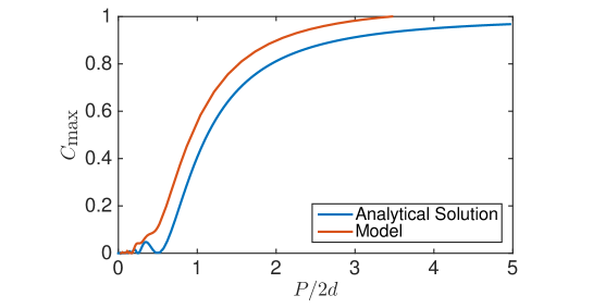
Figure 12: Normalised maximum cumulative $\text{CO}_{2}$ emissions for the analytical solution of equation (42), and the actual volcanic Green’s function from 6. The x-axis is sinusoidal sea level period divided by the width of the Green’s function.

However, MOR volcanism actually converges to a single value, independent of the Green’s function width, therefore this proposed $d^{2}$ scaling represents a divergence between our Green’s functions of MOR $\text{CO}_{2}$ emissions and the triangle function approximation. The difference is readily explained. As seen in figure 6a, for longer MOR lag times, the right-hand-side of the Green’s function triangle becomes increasingly concave compared to a hypothetical, symmetrical triangle function, causing less emissions than would be expected from the triangle function approximation. This difference is such that the Green’s functions all have the same total emissions in the long sea-level period limit.

Alternatively, explaining in physical terms, recall that sea-level-driven variable MOR $\text{CO}_{2}$ emissions are caused by the changing depth of first mantle melting. A low sea-level means a deeper depth of first melting, effectively flushing out $\text{CO}_{2}$ that would occupy mantle at that depth and inserting it into the atmosphere. There is a fixed density of $\text{CO}_{2}$ in that mantle, and thus a finite maximum $\text{CO}_{2}$ mass that a given amplitude of sea-level change can insert into the atmosphere, regardless of its period. Long-period sinusoidal sea level changes $P\gg d$ remove all the interference effects in upwelling melts arriving at the MOR and therefore all long-period sea level changes converge towards this same maximum $\text{CO}_{2}$ mass, regardless of MOR lag.

A.7 Tuning $C$ Feedback Strength

Equation (8) for carbon concentration in the atmosphere $C$ has three terms with corresponding sensitivity factors $\gamma_{\textrm{T}}$, $\gamma_{\textrm{MOR}}$, $\gamma_{\textrm{SAV}}$ controlling how much $C$ will change in response to changes in planetary temperature and sea level. In this section we run the model with only one $\text{CO}_{2}$ feedback term active, varying its corresponding sensitivity parameter, for each of the three feedback terms. The insolation forcing includes obliquity, precession and eccentricity. This demonstrates how the model behaves (with reconstructed insolation) when a particular $\text{CO}_{2}$ feedback is dominant .

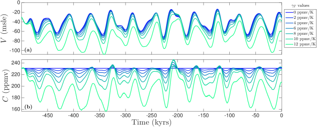
Figure 13: Increasing $\text{CO}_{2}$ temperature sensitivity parameter $\gamma_{\textrm{T}}$ with volcanic $\text{CO}_{2}$ effects turned off: $\gamma_{\textrm{MOR}},\gamma_{\textrm{SAV}}=0$. Panel (a) is ice volume in metres sea level equivalent. Panel (b) is $\text{CO}_{2}$ concentration in the atmosphere.

Figure 13 shows the model with $C$ responding only to changes in global average temperature: $\gamma_{\textrm{T}}\neq 0$ and $\gamma_{\textrm{MOR}},\gamma_{\textrm{SAV}}=0$. The amplitude of the glacial cycles increases with increasing positive feedback between $C$ and temperature, until the model enters a runaway glacial for $\gamma_{\textrm{T}}>12$ ppmv/K.

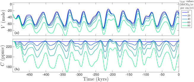
Figure 14: Increasing SAV $\text{CO}_{2}$ sensitivity to sea-level $\gamma_{\textrm{SAV}}$ with other $\text{CO}_{2}$ effects turned off: $\gamma_{\textrm{T}},\gamma_{\textrm{MOR}}=0$ Mt$\text{CO}_{2}$/yr per cm/yr. Panel (a) is ice volume in metres sea level equivalent. Panel (b) is $\text{CO}_{2}$ concentration in the atmosphere. The values in the legend are roughly equivalent to the peak increase in SAV $\text{CO}_{2}$ emissions flux caused by a deglaciation where $\dot{V}=1$ cm/yr.

Figure 14 has $C$ changing with variable SAV only: $\gamma_{\textrm{SAV}}\neq 0$ and $\gamma_{\textrm{T}},\gamma_{\textrm{MOR}}=0$. SAV $\text{CO}_{2}$ emissions lag the ice cycle by about 4 kyrs, and cause a runaway glacial for $\gamma_{\textrm{SAV}}\geq 90$ Mt$\text{CO}_{2}$/yr per cm/yr. As expected from the discussion of short-timescale feedbacks in section 4.1, both $V$ and $C$ timeseries in figure 14 are similar to figure 13, and neither changes the dominant period of glacial cycles.

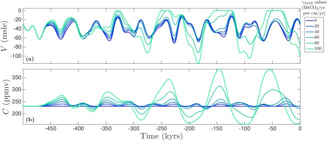
Figure 15: Increasing MOR $\text{CO}_{2}$ sensitivity to sea-level $\gamma_{\textrm{MOR}}$ with other $\text{CO}_{2}$ effects turned off: $\gamma_{\textrm{T}},\gamma_{\textrm{SAV}}=0$. Panel (a) is ice volume in metres sea level equivalent. Panel (b) is $\text{CO}_{2}$ concentration in the atmosphere. The values in the legend are roughly equivalent to the peak decrease in MOR $\text{CO}_{2}$ emissions flux caused by a deglaciation where $\dot{V}=1$ cm/yr.

Figure 15 has $C$ changing with variable MOR $\text{CO}_{2}$ emissions only ($40$ kyr MOR lag time): $\gamma_{\textrm{MOR}}\neq 0$ and $\gamma_{\textrm{T}},\gamma_{\textrm{SAV}}=0$. As with $\gamma_{\textrm{T}}$ and $\gamma_{\textrm{SAV}}$, increasing the $C$ sensitivity parameter $\gamma_{\textrm{MOR}}$ increases the amplitude of $C$ cycles. However, the response in ice volume is more complex; as $\gamma_{\textrm{MOR}}$ is increased, different maxima and minima in $V$ become more extreme or suppressed. This occurs because, as in section 4.1, the MOR-based variability in $C$ opposes some insolation-driven changes in $V$ (and reinforces others). As $\gamma_{\textrm{MOR}}$ increases further, the model moves towards glacial cycles at a multiple of the obliquity cycle: for $\gamma_{\textrm{MOR}}=80$ Mt$\text{CO}_{2}$/yr per cm/yr a $\sim$100 kyr oscillation dominates in the final 300 kyrs of $C$ (fig 15b).

These results for varying $C$ terms in eqn (8) are consistent with our suggestion that feedbacks need at least a $30$ kyr lag time to disrupt 40 kyr glacial cycles. This reinforces the conclusions from exploring varying MOR lag times in section 4.1.

Collectively, the results presented so far imply that variable MOR $\text{CO}_{2}$ emissions can change both the amplitude and periodicity of glacial cycles in $C$ and $V$, and the short-timescale carbon feedbacks from subaerial volcanism and the surface system only change the amplitude of glacial cycles. However, the increased amplitude of sea level change causes increased amplitude of cumulative MOR CO₂ emissions, therefore when all $\text{CO}_{2}$ feedbacks are active in the model the short-timescale feedbacks will affect when the model generates $\sim$100 kyr cycles.

A.8 Model Response to Noise

The main text establishes the behaviour of the model as a deterministic system. We showed the model tends toward $40$ kyr glacials driven by insolation cycles, but transitions to glacials at a multiple of the $40$ kyr cycle if the MOR $\text{CO}_{2}$ emissions response to sea-level change is increased. This section explores the model response to noise, evaluating if the model’s glacial cycles are stable to stochastic forcing of key variables. Geological records show considerable noise at $\lesssim 500$ year periods. Would such noise affect model behaviour?

To test this, we add Gaussian white noise to a parameter, randomly changing its value at each timestep in the model. The noise timeseries was created using MATLAB’s wgn function. We applied this model perturbation independently to insolation (change solar constant) and precipitation rate (change $P_{c}$).

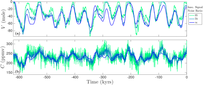
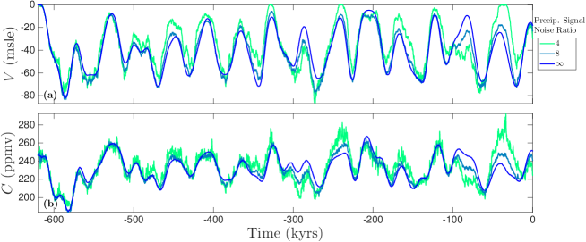
Figure 16: Model runs with increasing white noise added to insolation (upper pair) and precipitation (lower pair). In each pair the upper panel is ice volume in metres sea level equivalent and the lower panel is $\text{CO}_{2}$ concentration in the atmosphere. Noise is calculated by MATLAB’s wgn function with random seed 400. Signal to noise ratio is the standard deviation of the noise divided by default value of the perturbed parameter.

Figure 16 shows the results of stochastic forcing in both insolation (fig 16a,b) and precipitation (fig 16c,d). Both forcings show high-frequency perturbations in $V$ and $C$, despite the different physical mechanisms behind the perturbations. Insolation forcing changes the shortwave energy flux, thus changing Earth’s temperature and consequently causing both ice sheet growth/retreat and (via the $\gamma_{\textrm{T}}$ carbon feedback and WLC feedback term) $C$ changes. Precipitation forcing changes annual snowfall and thus directly affects ice sheet growth/retreat. The change in ice sheet extent changes surface albedo and consequently Earth’s temperature, leading to $C$ changes.

The stochastic forcings have no significant effect on SAV or MOR $\text{CO}_{2}$ emissions in the model, as the high-frequency variations in sea level (with a mean of zero) cancel out by the mechanism explained in section 3.1.

Neither insolation nor precipitation forcing significantly alters the $40$ kyr glacial cycle. These results hold for a range of random seeds and signal-to-noise ratios. Therefore high frequency noise similar to or greater than the geological record does not affect the key conclusions of this study.

References

- Abe-Ouchi et al. [2013] A. Abe-Ouchi, F. Saito, K. Kawamura, M. E. Raymo, J. Okuno, K. Takahashi, and H. Blatter. Insolation-driven 100,000-year glacial cycles and hysteresis of ice-sheet volume. Nature, 500(7461):190–193, Aug. 2013.
- Adams and Faure [1998] J. M. Adams and H. Faure. A new estimate of changing carbon storage on land since the last glacial maximum, based on global land ecosystem reconstruction. Global and Planetary Change, 17:3–24, May 1998.
- Archer et al. [2009] D. Archer, M. Eby, V. Brovkin, A. Ridgwell, L. Cao, U. Mikolajewicz, K. Caldeira, K. Matsumoto, G. Munhoven, A. Montenegro, and K. Tokos. Atmospheric Lifetime of Fossil Fuel Carbon Dioxide. dx.doi.org, 37(1):117–134, Apr. 2009.
- Arrhenius [1896] S. Arrhenius. On the influence of carbonic acid in the air upon the temperature of the ground. Phil. Mag., 41(251):237–276, 1896.
- Bereiter et al. [2015] B. Bereiter, S. Eggleston, J. Schmitt, C. Nehrbass-Ahles, T. F. Stocker, H. Fischer, S. Kipfstuhl, and J. Chappellaz. Revision of the EPICA Dome C CO 2record from 800 to 600 kyr before present. Geophysical Research Letters, 42(2):542–549, Jan. 2015.
- Berger and Loutre [1991] A. Berger and M. F. Loutre. Insolation values for the climate of the last 10 million years. Quaternary Science Reviews, 10(4):297–317, Jan. 1991.
- [7] Berkeley Earth Surface Temperatures. Monthly mean land surface temperatures 1951–80, 1 degree grid. file: Raw_tavg_equalarea.nc. http://berkeleyearth.org/data/m. Accessed: 2017-05-03.
- Bianchi et al. [2010] D. Bianchi, J. L. Sarmiento, A. Gnanadesikan, R. M. Key, P. Schlosser, and R. Newton. Low helium flux from the mantle inferred from simulations of oceanic helium isotope data. Earth and Planetary Science Letters, 297(3-4):379–386, Sept. 2010.
- Bony et al. [2015] S. Bony, B. Stevens, D. M. W. Frierson, C. Jakob, M. Kageyama, R. Pincus, T. G. Shepherd, S. C. Sherwood, A. P. Siebesma, A. H. Sobel, M. Watanabe, and M. J. Webb. Clouds, circulation and climate sensitivity. Nature Geoscience, 8(4):261–268, Apr. 2015.
- Braconnot and Kageyama [2015] P. Braconnot and M. Kageyama. Shortwave forcing and feedbacks in Last Glacial Maximum and Mid-Holocene PMIP3 simulations. Philosophical Transactions of the Royal Society a-Mathematical Physical and Engineering Sciences, 373(2054), 2015.
- Broecker et al. [2015] W. S. Broecker, J. Yu, and A. E. Putnam. Two contributors to the glacial CO2 decline. Earth and Planetary Science Letters, 429(C):191–196, Nov. 2015.
- Bryson et al. [2006] R. U. Bryson, R. A. Bryson, and A. Ruter. A calibrated radiocarbon database of late Quaternary volcanic eruptions. eEarth Discussions, 2006.
- Burley and Katz [2015] J. M. A. Burley and R. F. Katz. Variations in mid-ocean ridge CO2 emissions driven by glacial cycles. Earth and Planetary Science Letters, 426:246–258, Sept. 2015.
- Cai and Tung [2012] M. Cai and K.-K. Tung. Robustness of Dynamical Feedbacks from Radiative Forcing: 2 % Solar versus 2 x CO2 Experiments in an Idealized GCM. Journal of the Atmospheric Sciences, 69(7):2256–2271, July 2012.
- Cartigny et al. [2008] P. Cartigny, F. Pineau, C. Aubaud, and M. Javoy. Towards a consistent mantle carbon flux estimate: Insights from volatile systematics (H2O/Ce, delta D, CO2/Nb) in the North Atlantic mantle (14 degrees N and 34 degrees N). Earth and Planetary Science Letters, 265(3-4):672–685, 2008.
- Ciais et al. [2012] P. Ciais, A. Tagliabue, M. Cuntz, L. Bopp, M. Scholze, G. Hoffmann, A. Lourantou, S. P. Harrison, I. C. Prentice, D. I. Kelley, C. Koven, and S. L. Piao. Large inert carbon pool in the terrestrial biosphere during the Last Glacial Maximum. Nature Geoscience, 5(1):74–79, Jan. 2012.
- Clark and Pollard [1998] P. U. Clark and D. Pollard. Origin of the middle Pleistocene transition by ice sheet erosion of regolith. Paleoceanography, 13(1):1–9, Feb. 1998.
- Connolly et al. [2009] J. A. D. Connolly, M. W. Schmidt, G. Solferino, and N. Bagdassarov. Permeability of asthenospheric mantle and melt extraction rates at mid-ocean ridges. Nature, 462(7270):209–U83, 2009.
- Cronin and Tziperman [2015] T. W. Cronin and E. Tziperman. Low clouds suppress Arctic air formation and amplify high-latitude continental winter warming. Proceedings of the National Academy of Sciences, 112(37):11490–11495, Sept. 2015.
- Crowley et al. [2015] J. W. Crowley, R. F. Katz, P. Huybers, C. H. Langmuir, and S.-H. Park. Glacial cycles drive variations in the production of oceanic crust. Science, 347(6227):1237–1240, Mar. 2015.
- Crowley [1995] T. J. Crowley. Ice-Age Terrestrial Carbon Changes Revisited. Global Biogeochemical Cycles, 9(3):377–389, Sept. 1995.
- Cuffey and Vimeux [2001] K. M. Cuffey and F. Vimeux. Covariation of carbon dioxide and temperature from the Vostok ice core after deuterium-excess correction. Nature, 412(6846):523–527, 2001.
- Dasgupta and Hirschmann [2010] R. Dasgupta and M. M. Hirschmann. The deep carbon cycle and melting in Earth’s interior. Earth and Planetary Science Letters, 298(1-2):1–13, Sept. 2010.
- Donohoe et al. [2011] A. Donohoe, D. S. Battisti, A. Donohoe, and D. S. Battisti. Atmospheric and Surface Contributions to Planetary Albedo. dx.doi.org, 24(16):4402–4418, Aug. 2011.
- Elderfield et al. [2012] H. Elderfield, P. Ferretti, M. Greaves, S. Crowhurst, I. N. McCave, D. Hodell, and A. M. Piotrowski. Evolution of Ocean Temperature and Ice Volume Through the Mid-Pleistocene Climate Transition. Science, 337(6095):704–709, Aug. 2012.
- Ferrari et al. [2014] R. Ferrari, M. F. Jansen, J. F. Adkins, A. Burke, A. L. Stewart, and A. F. Thompson. Antarctic sea ice control on ocean circulation in present and glacial climates. Proceedings of the National Academy of Sciences, 111(24):8753–8758, June 2014.
- FISCHER [2008] T. P. FISCHER. Fluxes of volatiles (H2O, CO2, N2, Cl, F) from arc volcanoes. Geochemical Journal, 42(1):21–38, Feb. 2008.
- Fowler et al. [2013] A. C. Fowler, R. E. M. Rickaby, and E. W. Wolff. Exploration of a simple model for ice ages. GEM - International Journal on Geomathematics, 4(2):227–297, 2013.
- Franois et al. [1997] R. Franois, M. A. Altabet, E.-F. Yu, D. M. Sigman, M. P. Bacon, M. Frank, G. Bohrmann, G. Bareille, and L. D. Labeyrie. Contribution of Southern Ocean surface-water stratification to low atmospheric CO2 concentrations during the last glacial period. Nature, 389(6654):929–935, Oct. 1997.
- Galbraith and Eggleston [2017] E. D. Galbraith and S. Eggleston. A lower limit to atmospheric CO2 concentrations over the past 800,000 years. Nature Geoscience, 2017.
- Ganopolski and Calov [2011] A. Ganopolski and R. Calov. The role of orbital forcing, carbon dioxide and regolith in 100 kyr glacial cycles. Climate of the Past, 7(4):1415–1425, 2011.
- Gildor and Tziperman [2000] H. Gildor and E. Tziperman. Sea ice as the glacial cycles’ climate switch: Role of seasonal and orbital forcing. Paleoceanography, 2000.
- Goff et al. [2001] F. Goff, S. P. Love, R. Warren, D. Counce, J. Obenholzner, C. Siebe, and S. C. Schmidt. "passive infrared remote sensing evidence for large, intermittent co2 emissions at popocat̩petl volcano, mexico". Chemical Geology, 177(1):133 Р156, 2001. doi: 10.1016/S0009-2541(00)00387-9. High CO2 Flux Measurements in Volanic and Geothermal Areas, Methodologies and Results.
- Grant et al. [2014] K. Grant, E. Rohling, C. B. Ramsey, H. Cheng, R. Edwards, F. Florindo, D. Heslop, F. Marra, A. Roberts, M. E. Tamisiea, et al. Sea-level variability over five glacial cycles. Nature communications, 5, 2014.
- Harðardóttir et al. [2017] S. Harðardóttir, S. A. Halldórsson, and D. R. Hilton. Spatial distribution of helium isotopes in icelandic geothermal fluids and volcanic materials with implications for location, upwelling and evolution of the icelandic mantle plume. Chemical Geology, 2017.
- Harrison and Bartlein [2016] S. P. Harrison and P. J. Bartlein. What have we learnt from palaeoclimate simulations? Journal of Quaternary Science, 2016.
- Harrison et al. [2015] S. P. Harrison, P. J. Bartlein, K. Izumi, G. Li, J. Annan, J. Hargreaves, P. Braconnot, and M. Kageyama. Evaluation of CMIP5 palaeo-simulations to improve climate projections. Nature Climate Change, 5(8):735–743, Aug. 2015.
- Hönisch et al. [2009] B. Hönisch, N. G. Hemming, D. Archer, M. Siddall, and J. F. McManus. Atmospheric carbon dioxide concentration across the mid-pleistocene transition. Science, 324(5934):1551–1554, 2009.
- Hopcroft and Valdes [2015] P. O. Hopcroft and P. J. Valdes. How well do simulated last glacial maximum tropical temperatures constrain equilibrium climate sensitivity? Geophysical Research Letters, 2015.
- Huybers [2011] P. Huybers. Combined obliquity and precession pacing of late Pleistocene deglaciations. Nature, 480(7376):229–232, Dec. 2011.
- Huybers and Langmuir [2009] P. Huybers and C. Langmuir. Feedback between deglaciation, volcanism, and atmospheric CO2. Earth and Planetary Science Letters, 286(3-4):479–491, Sept. 2009.
- Huybers and Langmuir [2017] P. Huybers and C. H. Langmuir. Delayed CO 2 emissions from mid-ocean ridge volcanism as a possible cause of late-Pleistocene glacial cycles. Earth and Planetary Science Letters, 2017.
- Huybers and Tziperman [2008] P. Huybers and E. Tziperman. Integrated summer insolation forcing and 40,000-year glacial cycles: The perspective from an ice-sheet/energy-balance model. Paleoceanography, 23(1):–n/a, 2008.
- Imbrie and Imbrie [1980] J. Imbrie and J. Z. Imbrie. Modeling the Climatic Response to Orbital Variations. Science, 207(4434):943–953, 1980.
- IPCC [2013] IPCC. Climate change 2013: The physical science basis. contribution of working group i to the fifth assessment report of the intergovernmental panel on climate change. Book, Cambridge, United Kingdom and New York, NY, USA, 2013.
- Jellinek et al. [2004] A. M. Jellinek, M. Manga, and M. O. Saar. Did melting glaciers cause volcanic eruptions in eastern California? Probing the mechanics of dike formation. Journal of Geophysical Research-Solid Earth, 109(B9), 2004.
- Jull et al. [2002] M. Jull, P. B. Kelemen, and K. Sims. Consequences of diffuse and channelled porous melt migration on uranium series disequilibria. Geochimica et cosmochimica acta, 66(23):4133–4148, Dec. 2002.
- Keller et al. [2017] T. Keller, R. F. Katz, and M. M. Hirschmann. Volatiles beneath mid-ocean ridges: Deep melting, channelised transport, focusing, and metasomatism. Earth and Planetary Science Letters, 464:55–68, Apr. 2017.
- Köhler et al. [2010] P. Köhler, R. Bintanja, H. Fischer, F. Joos, R. Knutti, G. Lohmann, and V. Masson-Delmotte. What caused Earth’s temperature variations during the last 800,000 years? Data-based evidence on radiative forcing and constraints on climate sensitivity. Quaternary Science Reviews, 29(1-2):129–145, Jan. 2010.
- Kutterolf et al. [2013] S. Kutterolf, M. Jegen, J. X. Mitrovica, T. Kwasnitschka, A. Freundt, and P. J. Huybers. A detection of Milankovitch frequencies in global volcanic activity. Geology, 41(2):227–230, Feb. 2013.
- Larsen et al. [2001] C. Larsen, A. J. Newton, A. J. Dugmore, and E. G. Vilmundardottir. Geochemistry, dispersal, volumes and chronology of Holocene from the Katla volcanic silicic tephra layers system, Iceland. Journal of Quaternary Science, 16(2):119–132, Feb. 2001.
- Laskar et al. [2004] J. Laskar, P. Robutel, F. Joutel, M. Gastineau, A. Correia, and B. Levrard. A long-term numerical solution for the insolation quantities of the Earth. Astronomy & Astrophysics, 428(1):261–285, Dec. 2004.
- Le Voyer et al. [2017] M. Le Voyer, K. A. Kelley, E. Cottrell, and E. H. Hauri. Heterogeneity in mantle carbon content from CO2-undersaturated basalts. Nature Communications, 8:14062, 2017.
- Lisiecki and Raymo [2005] L. E. Lisiecki and M. E. Raymo. A Pliocene-Pleistocene stack of 57 globally distributed benthic delta O-18 records. Paleoceanography, 20(1), 2005.
- Lund and Asimow [2011] D. C. Lund and P. D. Asimow. Does sea level influence mid-ocean ridge magmatism on Milankovitch timescales? Geochemistry, Geophysics, Geosystems, 12(12):n/a–n/a, 2011.
- MacDonald [1990] G. J. MacDonald. Role of methane clathrates in past and future climates. Climatic Change, 1990.
- Maclennan et al. [2002] J. Maclennan, M. Jull, D. McKenzie, L. Slater, and K. Grönvold. The link between volcanism and deglaciation in Iceland. Geochemistry, Geophysics, Geosystems, 3(11):1–25, Nov. 2002.
- Martinez-Boti et al. [2015] M. A. Martinez-Boti, G. L. Foster, T. B. Chalk, E. J. Rohling, P. F. Sexton, D. J. Lunt, R. D. Pancost, M. P. S. Badger, and D. N. Schmidt. Plio-Pleistocene climate sensitivity evaluated using high-resolution CO2 records. Nature, 518(7537):49–+, 2015.
- Marty and Tolstikhin [1998] B. Marty and I. N. Tolstikhin. CO2 fluxes from mid-ocean ridges, arcs and plumes. Chemical Geology, 145(3-4):233–248, 1998.
- McKay et al. [2011] N. P. McKay, J. T. Overpeck, and B. L. Otto Bliesner. The role of ocean thermal expansion in Last Interglacial sea level rise. Geophysical Research Letters, 38(14):n/a–n/a, July 2011.
- Michael and Graham [2015] P. J. Michael and D. W. Graham. The behavior and concentration of CO2 in the suboceanic mantle: Inferences from undegassed ocean ridge and ocean island basalts. Lithos, 236-237:338–351, Nov. 2015.
- Middleton et al. [2016] J. L. Middleton, C. H. Langmuir, S. Mukhopadhyay, J. F. McManus, and J. X. Mitrovica. Hydrothermal iron flux variability following rapid sea level changes. Geophysical Research Letters, 43(8):3848–3856, Apr. 2016.
- Myhre et al. [1998] G. Myhre, E. J. Highwood, and K. P. Shine. New estimates of radiative forcing due to well mixed greenhouse gases. Geophysical research …, 1998.
- Oerlemans [1980] J. Oerlemans. Model Experiments on the 100,000-Yr Glacial Cycle. Nature, 287(5781):430–432, 1980.
- Olive et al. [2015] J. A. Olive, M. D. Behn, G. Ito, W. R. Buck, J. Escartin, and S. Howell. Sensitivity of seafloor bathymetry to climate-driven fluctuations in mid-ocean ridge magma supply. Science, 350(6258):310–+, 2015.
- Pagani et al. [2010] M. Pagani, Z. Liu, J. LaRiviere, and A. C. Ravelo. High Earth-system climate sensitivity determined from Pliocene carbon dioxide concentrations. Nature Geoscience, 3(1):27–30, Jan. 2010.
- Pierrehumbert et al. [2007] R. T. Pierrehumbert, H. Brogniez, and R. Roca. On the relative humidity of the Earth’s atmosphere. The General Circulation, 2007.
- Pollard [1982] D. Pollard. A simple ice sheet model yields realistic 100 kyr glacial cycles. Nature, 1982.
- Pollard [1983] D. Pollard. A coupled climate-ice sheet model applied to the Quaternary ice ages. Journal of Geophysical Research: Oceans, 1983.
- Rawson et al. [2015] H. Rawson, J. A. Naranjo, V. C. Smith, and K. Fontijn. The frequency and magnitude of post-glacial explosive eruptions at Volcán Mocho-Choshuenco, southern Chile. Journal of Volcanology …, 2015.
- Rawson et al. [2016] H. Rawson, D. M. Pyle, T. A. Mather, V. C. Smith, and K. Fontijn. The magmatic and eruptive response of arc volcanoes to deglaciation: Insights from southern Chile. …, 2016.
- Raymo et al. [2006] M. E. Raymo, L. E. Lisiecki, and K. H. Nisancioglu. Plio-pleistocene ice volume, Antarctic climate, and the global delta O-18 record. Science, 313(5786):492–495, 2006.
- Resing et al. [2004] J. A. Resing, J. E. Lupton, R. A. Feely, and M. D. Lilley. CO2 and 3He in hydrothermal plumes: implications for mid-ocean ridge CO2 flux. Earth and Planetary Science Letters, 226(3-4):449–464, Oct. 2004.
- Rind et al. [1995] D. Rind, R. Healy, C. Parkinson, and D. Martinson. The Pole of Sea-Ice in 2x Co2 Climate Model Sensitivity .1. the Total Influence of Sea-Ice Thickness and Extent. Journal of Climate, 8(3):449–463, Mar. 1995.
- Rohling et al. [2009] E. J. Rohling, K. Grant, M. Bolshaw, A. P. Roberts, M. Siddall, C. Hemleben, and M. Kucera. Antarctic temperature and global sea level closely coupled over the past five glacial cycles. Nature Geoscience, 2(7):500–504, July 2009.
- Saal et al. [2002] A. E. Saal, E. H. Hauri, C. H. Langmuir, and M. R. Perfit. Vapour undersaturation in primitive mid-ocean-ridge basalt and the volatile content of Earth’s upper mantle. Nature, 419(6906):451–455, Oct. 2002.
- Siddall et al. [2010] M. Siddall, B. Hoenisch, C. Waelbroeck, and P. Huybers. Changes in deep Pacific temperature during the mid-Pleistocene transition and Quaternary. Quaternary Sci. Rev., 2010. doi: 10.1016/j.quascirev.2009.05.011.
- Siebert et al. [2002] L. Siebert, T. Simkin, and K. P. Volcanoes of the world. Univ of California Press, 2002.
- Sigman et al. [2010] D. M. Sigman, M. P. Hain, and G. H. Haug. The polar ocean and glacial cycles in atmospheric CO2 concentration. Nature, 466(7302):47–55, 2010.
- Soden and Held [2006] B. J. Soden and I. M. Held. An assessment of climate feedbacks in coupled ocean-atmosphere models. Journal of Climate, 19(14):3354–3360, July 2006.
- Stap et al. [2014] L. B. Stap, R. S. W. van de Wal, B. de Boer, R. Bintanja, and L. J. Lourens. Interaction of ice sheets and climate during the past 800 000 years. Climate of the Past, 10(6):2135–2152, 2014.
- Tarasov and Peltier [1997] L. Tarasov and W. R. Peltier. Terminating the 100 kyr ice age cycle. Journal of Geophysical Research: …, 1997.
- Toggweiler [1999] J. R. Toggweiler. Variation of atmospheric CO 2 by ventilation. Paleoceanography, 1999.
- Toggweiler [2008] J. R. Toggweiler. Origin of the 100,000-year timescale in Antarctic temperatures and atmospheric CO2. Paleoceanography, 23(2):n/a–n/a, June 2008.
- Tolstoy [2015] M. Tolstoy. Mid-ocean ridge eruptions as a climate valve. Geophysical Research Letters, 42(5):1346–1351, 2015.
- Tzedakis, P. C. . et al. [2017] Tzedakis, P. C. ., M. Crucifix, T. Mitsui, and E. W. Wolff. A simple rule to determine which insolation cycles lead to interglacials. Nature, 542(7642):427–+, 2017.
- Tziperman et al. [2006] E. Tziperman, M. E. Raymo, P. Huybers, and C. Wunsch. Consequences of pacing the Pleistocene 100 kyr ice ages by nonlinear phase locking to Milankovitch forcing. Paleoceanography, 21(4):1879, Dec. 2006.
- van de Wal et al. [2011] R. S. W. van de Wal, B. de Boer, L. J. Lourens, P. Koehler, and R. Bintanja. Reconstruction of a continuous high-resolution CO2 record over the past 20 million years. Climate of the Past, 7(4):1459–1469, 2011.
- Watson et al. [2000] A. J. Watson, D. Bakker, A. J. Ridgwell, and P. W. Boyd. Effect of iron supply on Southern Ocean CO2 uptake and implications for glacial atmospheric CO2. Nature, 2000.
- Weber et al. [2007] S. L. Weber, S. S. Drijfhout, and A. Abe-Ouchi. The modern and glacial overturning circulation in the Atlantic ocean in PMIP coupled model simulations. Climate of the …, 2007.
- Yuan and Romanowicz [2017] K. Yuan and B. Romanowicz. Seismic evidence for partial melting at the root of major hot spot plumes. Science, 357(6349):393–396, 2017.
- Zhao [2001] D. Zhao. Seismic structure and origin of hotspots and mantle plumes. Earth and Planetary Science Letters, 192(3):251–265, 2001.