Slow and Long-ranged Dynamical Heterogeneities in Dissipative Fluids
	Karina E. Avila,a,b Horacio E. Castillo,b Katharina Vollmayr-Lee,c and Annette Zippeliusa
	A two-dimensional bidisperse granular fluid is shown to exhibit pronounced long-ranged dynamical heterogeneities as dynamical arrest is approached. Here we focus on the most direct approach to study these heterogeneities: we identify clusters of slow particles and determine their size, $N_{c}$, and their radius of gyration, $R_{G}$. We show that $N_{c}\propto R_{G}^{d_{f}}$, providing direct evidence that the most immobile particles arrange in fractal objects with a fractal dimension, $d_{f}$, that is observed to increase with packing fraction $\phi$. The cluster size distribution obeys scaling, approaching an algebraic decay in the limit of structural arrest, i.e., $\phi\to\phi_{c}$. Alternatively, dynamical heterogeneities are analyzed via the four-point structure factor $S_{4}(q,t)$ and the dynamical susceptibility $\chi_{4}(t)$. $S_{4}(q,t)$ is shown to obey scaling in the full range of packing fractions, $0.6\leq\phi\leq 0.805$, and to become increasingly long-ranged as $\phi\to\phi_{c}$. Finite size scaling of $\chi_{4}(t)$ provides a consistency check for the previously analyzed divergences of $\chi_{4}(t)\propto(\phi-\phi_{c})^{-\gamma_{\chi}}$ and the correlation length $\xi\propto(\phi-\phi_{c})^{-\gamma_{\xi}}$. We check the robustness of our results with respect to our definition of mobility. The divergences and the scaling for $\phi\to\phi_{c}$ suggest a non-equilibrium glass transition which seems qualitatively independent of the coefficient of restitution.

1 Introduction

Supercooled liquids, colloidal suspensions, and granular systems show evidence of strong fluctuations as they approach dynamical arrest. These fluctuations are associated with the presence of cooperative dynamics, and in particular with the presence of dynamical heterogeneity: some regions are populated by more mobile particles, and relax much faster than other regions, which contain slower particles. Experiments and simulations agree that the heterogeneity becomes dramatically stronger when the glass transition is approached ^{1, 2, 4, 3, 5}. This phenomenon has been observed in structural glasses as well as in colloidal suspensions and granular materials.

Despite similarities on a phenomenological level, it is still controversial, how the glass transition ⁶ and the jamming transition ⁷ are related ^{8, 9, 10}. Whereas early work suggested a unified picture, more recent studies point to two separate transitions ¹⁰, one at finite $T$ and comparatively low density and the other one at $T=0$ and high density. Jamming without applied shear is a packing problem and hence the same for elastically and inelastically colliding hard particles. On the other hand, dissipation in particle-particle collisions causes the granular fluid to be inherently out of equilibrium – in contrast to a thermal glass which falls out of equilibrium at the glass transition. Hence it is important to understand to what degree the phenomenon of dynamical heterogeneity in non-equilibrium systems is comparable to the analogous phenomenon in ordinary structural or colloidal glasses. With the latter, granular fluids share the advantage that particle positions can be tracked over time, so that correlated dynamics is accessible to experiment.

We analyze data from event-driven numerical simulations of a homogeneously driven two-dimensional hard sphere system. This granular system resembles experiments performed on air tables. In those experiments ¹¹, air is injected into the system in order to restore the energy that is lost to dissipation in interparticle collisions. The systems we consider contain large numbers of particles, between $3.6\times 10^{5}$ and $4.0\times 10^{6}$. Thereby finite size effects are significantly reduced. Furthermore, large system sizes are a prerequisite to study fluctuations on large spatial scales which is at the heart of our study.

We observe a diverging relaxation time, $\tau_{\alpha}$, of the average overlap $Q(t)$, which allows us to identify a critical density, $\phi_{c}$. Time-density superposition is shown to be violated, but data for different packing fractions and coefficients of restitution can be collapsed with an empirical scaling function. We then use several approaches to analyze the growing range and strength of the dynamic heterogeneities as a function of packing fraction $\phi$:

• First, we identify clusters of slow and fast particles and compute the cluster size distribution as well as the average radius of gyration $R_{g}$.

• Second, we compute the dynamical susceptibility $\chi_{4}(t)$ measuring the number of correlated particles.

• Third, we analyze the growing length scale of dynamical heterogeneity by means of the four–point structure factor $S_{4}(q,t)$, which is the correlation function of the density at two different points for two different times. $S_{4}(q,t)$ obeys scaling and $\xi$ can be obtained from low $q$ behavior.

• Fourth, we use finite size scaling for $\chi_{4}(\tau_{\alpha})$ as a consistency check for the correlation length and the fractal dimension as obtained from the above approaches.

These results are interpreted in terms of a glass transition in a non–equilibrium fluid with pronounced dynamical heterogeneities. Particle displacements are strongly heterogeneous, as signaled by overpopulated tails in the distribution of particle displacements. The latter displays an exponential tail for times comparable or greater than $\tau_{\alpha}$. Clusters of slow particles are growing in size and number. The distribution of cluster sizes obeys scaling and approaches an algebraic decay as $\phi\to\phi_{c}$. Relating the radius of gyration to cluster size shows that clusters are fractals, which compactify as dynamical arrest is approached. The peak of the four-point susceptibility, $\chi_{4}(t)$, increases dramatically as $\phi\to\phi_{c}$ and simultaneously the time of occurrence of the peak increases, comparably to $\tau_{\alpha}$. Spatial fluctuations of the overlap are measured by $S_{4}(q,t)$, which obeys scaling, and allows us to extract a dynamic correlation length $\xi(t)$. Both $\chi_{4}(\tau_{\alpha})$ and $\xi(\tau_{\alpha})$ are found to diverge algebraically as $\phi\to\phi_{c}$, so that we obtain another estimate $d_{f}^{\prime}$ for the fractal dimension by relating average cluster size to the correlation length, $\chi_{4}(\tau_{\alpha})\propto\xi^{d_{f}^{\prime}}({\tau_{\alpha}})$. The resulting fractal dimension is independent of packing fraction – presumably because we do not resolve cluster sizes. Finite size scaling analysis for $\chi_{4}$ as a function of $\phi$ and $N$ provides a consistency check for the critical behavior of $\chi_{4}(\tau_{\alpha})$ and $\xi({\tau_{\alpha}})$. A short summary of some of our results has been published in ¹²

This paper is organized as follows. In Sec. 2 we describe the system and the simulation methods. In Sec. 3 we discuss our results, starting in 3.1 with the slowing down of the dynamics as quantified by the dynamic overlap. In Sec. 3.2 we present results for the distribution of particle displacements at different packing fractions. In Sec. 3.3, we analyze clusters of slow and fast particles in terms of the radius of gyration $R_{g}$ and the cluster size distribution. In Secs. 3.4 we analyze the dynamical susceptibility $\chi_{4}(t)$ and the correlation length $\xi(t)$ at $t=\tau_{\alpha}$ as functions of the packing fraction. We explore the dependence of $\chi_{4}$ and $\xi$ on (i) the system size $N$, (ii) the time difference $t$, (iii) the cutoff parameter $a$ of the overlap function, and (iv) the coefficient of restitution $\varepsilon$. We confirm that the results for $\xi$ are robust with respect to details of the analysis such as $a$, the fit range and the fitting function for $S_{4}(q,t)$. Finally, in Sec. 4 we discuss our conclusions.

2 Model and Simulation details

The model consists of a 2D system of hard disks which only interact via two-body inelastic (or elastic) collisions, without a rotational degree of freedom. The system is composed of particles of two sizes with a $50:50$ composition, i.e., it is bidisperse. The ratio of particle radii is given by $r_{2}/r_{1}\approx 1.43$, where $r_{1}$ denotes the radius of the small particles and $r_{2}$ denotes the radius of the large particles. This is the same system as the one presented in Ref. ¹³, which can also be consulted for additional details of the simulation.

The change in the velocities of two colliding particles, particle i and particle j, is given by

$$({\bf g}\cdot{\bf n})^{{}^{\prime}}=-\varepsilon({\bf g}\cdot{\bf n}),$$ (1)

where ${\bf g={\bf v}_{i}}-{\bf v}_{j}$ is the relative velocity, ${\bf n}=({\bf r}_{i}-{\bf r}_{j})/|{\bf r}_{i}-{\bf r}_{j}|$ is a unit vector that connects the center of the two disks and $\varepsilon$ corresponds to the coefficient of restitution, which is constant ($\varepsilon=1$ in the elastic case). The primed quantities refer to post-collisional velocities while the unprimed ones refer to pre-collisional velocities. Therefore, the velocities of the two disks after a collision are given by

$$m_{i}{\bf v}^{{}^{\prime}}_{i}=m_{i}{\bf v}_{i}-\frac{m_{i}m_{j}}{m_{i}+m_{j}}(1+\varepsilon)({\bf g}\cdot{\bf n}){\bf n}$$ (2)

and

$$m_{j}{\bf v}^{{}^{\prime}}_{j}=m_{j}{\bf v}_{j}+\frac{m_{i}m_{j}}{m_{i}+m_{j}}(1+\varepsilon)({\bf g}\cdot{\bf n}){\bf n},$$ (3)

where $m_{i}$ corresponds to the mass of particle $i$. In our simulations, constant mass density is assumed for all particles, therefore the mass ratio of the particles is given by $m_{2}/m_{1}=(r_{2}/r_{1})^{2}$.

In these systems, the driving of the particles is important to compensate the energy dissipation due to collisions. In experiments, this driving can be done by various methods, for example by shearing the boundaries ⁴, by applying frictional forces through a moving surface that is in contact with the particles ^{14, 15}, or by blowing an air current through the system ¹⁶. In our simulations, the energy is fed homogeneously by bulk driving, in a way that is comparable to the bulk driving in ¹⁶. Energy is fed to the system by applying instantaneous “kicks” to randomly chosen pairs of particles. For each particle in the pair, the velocity changes according to

$$m_{i}{\bf v}^{{}^{\prime}}_{i}(t)=m_{i}{\bf v}_{i}(t)+p_{Dr}{\bf\kappa}_{i}(t),$$ (4)

where $p_{Dr}$ is the driving amplitude and ${\bf\kappa}_{i}(t)$ is a Gaussian random vector giving the direction of the driving. The two particles are given opposite momenta of equal magnitude to ensure conservation of the total momentum of the system ¹⁷. The magnitude of the kick, $p_{Dr}^{2}=(1-\varepsilon^{2})\frac{m_{1}m_{2}}{m_{1}+m_{2}}$, is chosen to vanish in the elastic limit. The driving frequency is chosen to be equal to the Enskog collision frequency, $\omega_{\text{coll}}=2.59\phi G_{c}\sqrt{(}1/\pi)$, where $G_{c}$ is the pair correlation at contact (for details see Refs. ^{18, 13}). All results shown in this paper are presented in reduced units, where the length unit corresponds to $r_{1}$ and the mass unit correspond to $m_{1}$. Also, the time unit is set such that the kinetic energy, averaged over all the particles, is unity: $\frac{1}{2N_{\text{tot}}}\sum_{i}^{N_{\text{tot}}}m_{i}{{\bf v}_{i}}^{2}(t=0)=1$.

In this work, we analyze several simulation datasets. Some of the simulations were performed on a system containing $N_{\text{tot}}=4,000,000$ particles, for the packing fractions $\phi=0.60$, $0.65$, $0.70$, $0.72$, $0.74$, $0.76$ and $0.78$, which were also used in Ref. ¹³ in a different analysis, and $N_{\text{tot}}=360,000$ for the higher packing fractions $\phi=0.805$, $0.80$, $0.795$, $0.79$, $0.785$ and $0.77$. We performed simulations for all packing fractions mentioned above for the coefficient of restitution $\varepsilon=0.90$. Also, we have additional simulations, for $\phi=0.79$, $0.78$, $0.76$, $0.74$ and $0.72$ for $\varepsilon=1.00$, $0.80$ and $0.70$. Moreover, for each packing fraction $\phi$ we select for the analysis the time window such that the system is in a steady state.

2.1 Averages in our results

Before introducing our results, this section is dedicated to explaining the main procedures used to analyze our data and specify the notation for spatial and temporal averages.

Sub–box analysis: When probing spatial heterogeneities, we need to compute fluctuations of two-point correlations, such as fluctuations of the incoherent van Hove function. In order to do so, we divide our simulation box of total area $(L_{\text{tot}})^{2}$, which contains the $N_{\text{tot}}$ particles, into sub-boxes $B_{\bf{r}}$ of equal area $L^{2}$, as shown in Fig. 1. We select $L$ such that the sub–boxes accommodate, on average, a desired number of particles $N$, depending on the analysis performed. The choice of $N$ will be specified in each case. However, even when $N$ is fixed, the number of particles per sub–box, $N_{{\bf r}}$, and the particle concentration of big and small particles in general vary between different sub–boxes. The notation $N_{{\bf r}}$ denotes the number of particles of a sub–box centered at a point ${\bf r}$.

Fig.  1: The simulation box, of total area $(L_{\text{tot}})^{2}$, contains $N_{\text{tot}}$ particles, and is divided into sub–boxes of area $L^{2}$. Each sub-box contains a number $N_{{\bf r}}$ of particles, that fluctuates in different sub–boxes.

Notice that the total number of sub–boxes can be calculated as the ratio $N_{\text{tot}}/N$. In general, the more particles $N_{\text{tot}}$, the better the statistics in the analysis. The spatial average over the whole sample is denoted by $\langle\cdots\rangle$.

Time average. Besides space averaging, we use time averaging for some calculations to improve the statistics, especially for the packing fractions $\phi=0.77$, $0.785$, $0.79$, $0.795$, $0.80$ and $0.805$, for which the system contains fewer particles than for the rest of the packing fractions. Time averages are denoted by $\overline{\cdots}$. It is worth noting that time averaging is possible because the simulations are done in the stationary state, i.e., the system is not aging. This means that an average over different choices of the starting time $t_{0}$ can be performed for quantities that have a dependence on the time difference.

3 Results

3.1 Overlap

Before we examine dynamic heterogeneities, i.e., four-point correlations, let us first look at the relaxation of the system and the relevant time-scales associated with this relaxation. We begin with the two-point correlation, the overlap

$$Q_{\bf r}(t;t_{0})=\frac{1}{N}\sum_{i=1}^{N_{{\bf r}}}\theta(a-|{\bf r}_{i}(t_{0}+t)-{\bf r}_{i}(t_{0})|),$$ (5)

where ${\bf r}_{i}(t)$ is the position of particle $i$ at time $t$ and $\theta(x)$ is the Heaviside theta function, $\theta(x)=1$ for $x>0$ and $\theta(x)=0$ for $x<0$. The sum runs over particles $i=1,\ldots,N_{\bf r}$ which are at time $t_{0}$ in a sub–box $B_{\bf r}$ of size $L^{2}$ centered at ${\bf r}$. Here $N_{\bf r}$ is the actual number of particles in the region at time $t_{0}$ and $N\equiv\langle N_{\bf r}\rangle$ is the average number of particles for a region of the given size. We refer to those particles that moved less than a given cutoff distance $a$ over the time interval between $t_{0}$ and $t_{0}+t$ as slow particles. The overlap $Q_{\bf r}(t;t_{0})$ is therefore the ratio between the number of slow particles in the sub–box centered at ${\bf r}$ and the average number of particles in the region, and hence a fluctuating quantity. We will study its fluctuations in Sec. 3.4, but first discuss its average to identify the relevant timescale and discuss the relaxation to a stationary state.

We want to make sure that the system has relaxed to a stationary state before taking measurements. The required relaxation time, $\tau_{\text{stat}}$, is comparable to $\tau_{\alpha}$, defined by $Q_{r}(\tau_{\alpha},t_{0})=1/e$. Typically we take $\tau_{\text{stat}}\geq 9\tau_{\alpha}$. To check that this is indeed sufficient we consider the average over subboxes

$$Q(t;t_{0})=\left<Q_{\bf r}(t;t_{0})\right>,$$ (6)

which in general still depends on two times: the waiting time $t_{0}$ which elapses after relaxation and before taking measurements and the time difference $t$. In the stationary state this function should not depend on $t_{0}$ anymore. In Fig. 2 we show $Q(t;t_{0})$ for packing fraction $\phi=0.78$ and many waiting times $t_{0}$.

Fig.  2: Overlap, $Q(t;t_{0})$, for $\phi=0.78$ and several waiting times $t_{0}$; inset: relaxation time $\tau_{\alpha}$, defined by $Q(\tau_{\alpha},t_{0})=1/e$ as a function of $t_{0}$ for two packing fractions $\phi=0.78$, and $0.805$.

The function $Q(t;t_{0})$ is indeed independent of $t_{0}$, in other words no aging is observed. We have checked this for all densities and show $\tau_{\alpha}$ as a function of $t_{0}$ in the inset for $\phi=0.78$ and $0.805$.

Given that we are in a stationary state, we average the overlap over time

$$Q(t)=\overline{\left<Q_{\bf r}(t;t_{0})\right>},$$ (7)

which is shown in Fig 3. (We always choose $a=0.6$ and $\varepsilon=0.9$, unless stated otherwise).

Fig.  3: Slowdown of the overlap function, $Q(t)$, for packing fractions (left to right) $\phi=0.60,0.65,0.70,0.72$, $0.74,0.76,0.77$, $0.78,0.785,0.79,0.795,0.80,0.805$; the horizontal line corresponds to the value of the correlation function, $Q(\tau_{\alpha})=1/e$, defining $\tau_{\alpha}$.

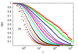
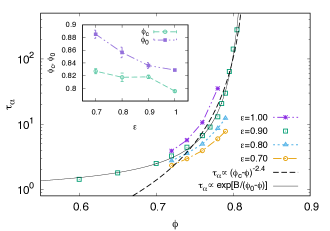
In contrast to three-dimensional systems, there is almost no two-step relaxation ^{13, 23}, instead the decay of $Q(t)$ just slows down progressively as the packing fraction $\phi$ is increased. To quantify this slowdown, we show in Fig. 4 the relaxation time $\tau_{\alpha}$ as a function of $\phi$, where $\tau_{\alpha}$ is defined by $Q(\tau_{\alpha})={\rm 1/e}$.

Fig.  4: Dependence of the relaxation time on $\phi$. Two possible fits, $\tau_{\alpha}\propto(\phi_{c}-\phi)^{-\gamma_{\tau}}$ (dashed line) and $\tau_{\alpha}\propto\exp{[B/(\phi_{0}-\phi)]}$ (solid line), are shown.

Included in Fig. 4 are two fits: one to an inverse power law $\tau_{\alpha}\propto(\phi_{c}-\phi)^{-\gamma_{\tau}}$ (dashed line) as predicted by mode coupling theory ^{19, 20}, and another to an exponential form $\tau_{\alpha}\propto\exp{[B/(\phi_{0}-\phi)]}$ (solid line). Both fitting forms extrapolate to a divergence of $\tau_{\alpha}$, located at $\phi\to\phi_{c}=0.82$ and at $\phi\to\phi_{0}=0.83$ respectively. The exponential fit describes the curve better across the whole $\phi$ range than the inverse power law, which only works for a narrower range of values of $\phi$. This behavior has been also found in other systems (see for example ^{21, 22}).

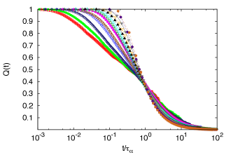
Thus, our results so far are similar to previous work on glass dynamics. Unexpected differences, however, occur in the shape of the $Q(t)$ decay. In Fig. 5 we test time-density superposition, i.e., whether $Q(t)$ for different $\phi$ is scaling with $t/\tau_{\alpha}(\phi)$. Clearly, time-density superposition does not give rise to a good data collapse for granular fluids in 2D. Similarly, in ²³ it was found that for a 2D non–dissipative glassy system time–temperature superposition fails, while in a similar 3D system it holds.

Fig.  5: The overlap $Q$ as in Fig. 3 but here as a function of $t/\tau_{\alpha}$ to demonstrate the breakdown of time-density superposition (color coding as in Fig. 3).

Despite the absence of time-density superposition, a simple description of the relaxation functions is possible. We have fitted $Q(t)$ with the empirical form

$$Q(t)=\frac{1}{\exp[\beta\ln(t/\tau_{0})]+1}=\frac{1}{\left({t}/{\tau_{0}}\right)^{\beta}+1},$$ (8)

where the exponent $\beta$ and the characteristic time $\tau_{0}$ are fitting parameters that depend on $\varepsilon$ and $\phi$. Fig. 6 is a scaling plot of $Q(t)$ as a function of $x\equiv\beta\ln(t/\tau_{0})$, for all simulated values of packing fraction $\phi$ and coefficients of restitution $\varepsilon$ (see below for a discussion of variations of $\varepsilon$). The numerical results for different densities and restitution coefficients show a remarkably good collapse.

Fig.  6: $Q(t)$ fitted to Eq. (8) with fit parameters $\tau_{0}(\phi)$ and $\beta(\phi)$, for all simulated values of $\phi$ and $\varepsilon$; dashed line indicates the algebraic time dependence, $(t/\tau_{0})^{-\beta}$ for $t>\tau_{\alpha}$. The inset shows that $\beta(\tau_{0})$ and $\tau_{\alpha}(\tau_{0})$ follow power laws for $\varepsilon=0.90$.

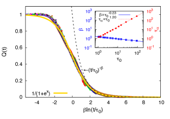
Both, $\beta$ as well as $\tau_{0}$, follow a power law as a function of $\tau_{\alpha}$ (see inset of Fig. 6).

The collapse of the data to the empirical scaling function Eq. (8), implies an algebraic decay $\propto(t/\tau_{0})^{-\beta}$ for times $t\geq\tau_{\alpha}$ as indicated in Fig. 6.

3.2 Heterogeneous Particle Displacements

Next we investigate the heterogeneity in the particle displacement. Whereas in the following section we will study the spatial distribution of “fast” and “slow” particles, we quantify in this section the disparity between fast and slow particles.

Fig.  7: MSD for different subsets of particles, either restricted to small particles (dashed lines) or for all particles (solid lines) for packing fraction $\phi=0.78$; the upper curves corresponds to the fastest particles, the middle curves to all particles and the lower ones to the slowest particles.

Fig.  8: (a) Distribution of small particle displacements for different packing fractions $\phi=0.805$, $0.78$, and $0.60$ (from right to left) at time $\tau_{\alpha}$. (b) Distribution of small particle displacements for $\phi=0.78$ at different times $t=0.01\tau_{\alpha}$, $t=\tau_{\alpha}$ and $t=8.5\tau_{\alpha}$ (from left to right). The tails of the distributions are better described by an exponential fit (solid lines) than by a gaussian fit (dotted-dashed lines).

Fig.  9: Diffusion coefficient $D$ as a function of $\tau_{\alpha}$ for different values of $\phi$, demonstrating the breakdown of the Stokes-Einstein relation as shown as a dotted line. Instead we observe a crossover from $D\propto{\tau_{\alpha}}^{-\theta}$ at intermediate densities (solid line) to $D\propto{\tau_{\alpha}}^{-\theta^{\prime}}$ at the highest densities (dashed line).

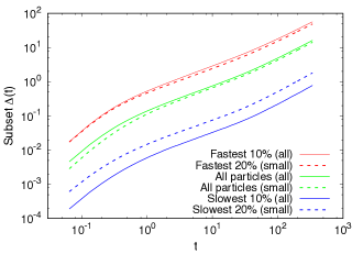
Fig. 7 shows the mean square displacement (MSD) for all particles (green solid line) and for small particles (green dashed–dotted line) given by

$$\Delta(t)=\frac{1}{N_{\text{set}}}\sum_{i=1}^{N_{\text{set}}}({\bf r}_{i}(t_{0}+t)-{\bf r}_{i}(t_{0}))^{2},$$ (9)

where $N_{\text{set}}$ is the total number of particles belonging to the subset considered, i.e., $N_{\text{set}}=N_{\text{tot}}$ for all particles (see Sec. 2.1 for the definition of $N_{\text{tot}}$) and ${\bf r}_{i}(t)$ is the position of particle i at time $t$. We furthermore show in Fig. 7 the MSD as a function of time $t$ for subsets defined based on the instantaneous particles‘ MSD

- the fastest $10\%$ of all particles (red full line),

- the fastest $20\%$ of small particles (red dashed line),

- the slowest $10\%$ of all particles (blue full line),

- the slowest $20\%$ of small particles (blue dashed line)

and compare them to the corresponding quantities for all particles. Note that the sets of the slowest (fastest) $10\%$ refer here to an instant of time $t$ or rather a small interval $[t,t+\Delta t]$. For each small time interval $\Delta t$ the selected subset is in general different. Therefore, many of the particles which are among the slowest $10\%$ for a certain time interval will not be among the slowest $10\%$ for other (shorter or longer) time intervals.

We find, in accordance with Fig. 13 of ¹³, a vast difference between fast and slow particles. While the 10% fastest particles move a distance several times the radius $r_{1}$ of the small particles, the slowest 10% of particles barely move. The restriction to small particles does not significantly change this observation. The drastic differences of particle mobility give us an idea of the strength of the dynamical heterogeneity.

The full distribution of displacements in the $x$-direction, $\Delta x(t)=[x_{i}(t_{0}+t)-x_{i}(t_{0})]$ at a fixed time difference $t$ is shown in Fig. 8(a) for various packing fractions and in Fig. 8(b) for several times $t$. For a fluid far from dynamical arrest, the particles are expected to perform a simple random walk, and the displacement distributions are expected to have a Gaussian form $P_{g}(\Delta x,t)=\left(1/\sqrt{4\pi Dt}\right)\exp[-(\Delta x)^{2}/(4Dt)]$, where $D$ is the diffusion coefficient. Gaussian fits to the data, with $D$ used as a fitting parameter, are shown with dotted-dashed lines in Fig. 8. We observe that the distributions deviate strongly from the Gaussian fit for all packing fractions and times. The tails of the distributions follow approximately exponential behavior, $P_{e}(\Delta x,t)\propto\exp(-|(\Delta x)/x_{0}(t)|)$, shown as solid lines. Also, the tails become wider both for increased packing fraction and for longer times. Exponential tails have been studied also in non-dissipative glassy systems ^{24, 25, 26} and have been established as an indirect signature of spatial dynamical heterogeneity ²⁶.

Another expected consequence of the presence of heterogeneous dynamics is that supercooled liquids near the glass transition in 3D violate both the Stokes-Einstein relation $D\eta/T=const$ ^{1, 2} connecting the diffusion coefficient $D$ with the viscosity $\eta$, and the related condition $D\tau_{\alpha}/T=const^{\prime}$ connecting $D$ with the $\alpha$-relaxation time $\tau_{\alpha}$. Both ratios, $D\eta/T$ and $D\tau_{\alpha}/T$, show strong increases as the liquid approaches dynamical arrest. In two dimensional thermal systems, a different phenomenology has been found ²⁷: both ratios behave as power laws as functions of temperature, even far from dynamical arrest, but the exponents for the power laws show significant changes as the liquid goes from the normal regime to the supercooled regime.

In our case, we focus on the relation between $D$ and $\tau_{\alpha}$. We obtain the values of $D$ by fitting the long time limit of the MSD (see Eq. (9)) with the form $\Delta(t)=4Dt$. This is known to be problematic in 2D, because long time tails of the velocity autocorrelation threaten the existence of hydrodynamics ¹³. However, these tails are strongly suppressed in the vicinity of the glass transition, so that the above naive definition of $D$ is presumably only weakly – if at all – affected.

Fig. 9 is a plot of $D$ as a function of $\tau_{\alpha}$, for all values of $\phi$. For packing fractions not too close to dynamical arrest, a power law behavior $D\propto{\tau_{\alpha}}^{-\theta}$ is found, with $\theta\approx 1.47$.

Fig.  10: Spatial distribution of slow and fast particles. Slow particles, which had a displacement shorter than $a$ in one relaxation time are shown in red (dark gray), fast particles, which had a displacement longer than $3a$ in one relaxation time are shown in gray (light gray). Here $\varepsilon=0.9$, $a=0.6$, and the different panels correspond to different packing fractions: (a) $\phi=0.60$, (b) $\phi=0.78$ and (c) $\phi=0.805$.

For higher packing fractions, one observes a crossover to a power law with a different exponent, $\theta^{\prime}\approx 0.91$. These results confirm the breakdown of the Stokes-Einstein relation for small $\tau_{\alpha}$, i.e., far away from the glass transition, which has also been observed ²⁷ in 2D non-dissipative glass forming systems.

3.3 Clusters of slow and fast particles

In this section we investigate directly the spatial distribution of dynamical heterogeneities. We look at the whole system as one unit, instead of dividing it into sub-boxes.

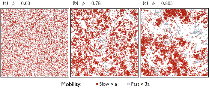
To visually observe dynamical heterogeneity in our system we color–code particles according to their mobility. As in Sec. 3.1, we define slow particles as those that for a given time interval $t$ have a displacement smaller than the cutoff $a$. Additionally, we define fast particles as those that in the same time interval have a displacement larger than $3a$. The spatial distribution of slow and fast particles is shown in Fig. 10, for $\varepsilon=0.9$ and three different packing fractions, for a time interval $t=\tau_{\alpha}$ corresponding to the $\alpha-$relaxation time. The fast particles are displayed in gray (light gray) and the slow particles in red (dark gray). We observe that both slow and fast particles form clusters, and that in both cases the typical size of the clusters increases as the packing fraction increases.

We now analyze quantitatively the size and shape of those clusters for several packing fractions $\phi$ at time difference $\tau_{\alpha}$. For each packing fraction we use several snapshots of the system, generated starting from different initial condition. Unless otherwise indicated, all results in this analysis are for $\varepsilon=0.9$ and $a=0.6$.

Two slow/fast particles belong to the same cluster if they are linked by a chain of nearest neighbor pairs of slow/fast particles. Since the particles are distributed continuously in space, there is some ambiguity in the definition of what constitutes a pair of nearest neighbors. By convention, we say that two particles are nearest neighbors if they are separated by a distance smaller than $r^{\rm min}_{\alpha\beta}$, where $r^{\rm min}_{\alpha\beta}$ is the position of the first minimum of the radial pair distribution $g_{\alpha\beta}(r)$ for particles $\alpha,\beta\in\{1,2\}$ (see Fig. 14 and Fig. 15 in ¹³).

Let’s consider one of the clusters in the system. In order to quantify its size and shape, we define $N_{c}$ as the number of particles in the cluster and its radius of gyration by

$$R_{g}=\left[\frac{1}{N_{c}}\sum_{i=1}^{N_{c}}|{\bf r}_{i}(\tau_{\alpha})-{\bf R}_{CM}(\tau_{\alpha})|^{2}\right]^{1/2},$$ (10)

where ${\bf r}_{i}(\tau_{\alpha})$ for $i=1,\cdots,N_{c}$ are the positions of the particles that belong to the cluster, and ${\bf R}_{CM}(t)\equiv N_{c}^{-1}\sum_{i=1}^{N_{c}}{\bf r}_{i}(t)$ is the position of the cluster’s center of mass.

Fig.  11: Radius of gyration $R_{g}$ as a function of cluster size $N_{c}$ for $\phi=0.805$. A power law fit of the data to $R_{g}\propto{N_{c}}^{1/d_{f}}$ gives the values $d_{f}\approx 1.91$ for (a) slow clusters and $d_{f}\approx 1.73$ for (b) fast clusters. The inset of (a) shows the fractal dimension $d_{f}$ for clusters of slow particles as a function of $\phi$.

To characterize all of the clusters of slow/fast particles that are present at a given time we show $R_{g}(N_{c})$ for $\phi=0.805$ in Fig. 11(a) for slow clusters and in Fig. 11(b) for fast clusters. We notice that there are many slow clusters with $N_{c}>10^{3}$, and even some with $N_{c}>10^{4}$.

The relationship between the radius of gyration and the cluster size can be described by a power law of the form $R_{g}\propto{N_{c}}^{1/d_{f}}$, where $d_{f}$ corresponds to the fractal dimension of the clusters, i.e., characterizes the shape of the clusters. For the packing fraction shown in Fig. 11 we obtained a value $d_{f}\approx 1.91$ for slow clusters and $d_{f}\approx 1.73$ for fast clusters.

The inset of Fig. 11(a) shows the fractal dimension $d_{f}$ as a function of the packing fraction $\phi$, for slow clusters ²⁸. For slow clusters the value of $d_{f}$ increases with $\phi$ from a value $d_{f}\approx 1.65$ for $\phi=0.60$ to a value $d_{f}\approx 1.91$ for $\phi=0.805$. This result suggests that the slow clusters exhibit a more compact shape when approaching dynamical arrest, as also suggested by Fig. 10(c).

Fig.  12: Cluster size distribution $P(N_{c})$ for different packing fractions $\phi$. (a) The distribution $P(N_{c})$ of slow clusters follows a power law $P(N_{c})\propto{N_{c}}^{-1.8}$ up to the cluster size $N^{*}$, which increases with increasing $\phi$. (b) Distribution of fast clusters.

Fig.  13: Collapse of the data for slow clusters using the scaling ansatz $P(N_{c})\sim N_{c}^{-\kappa}f(N_{c}/N^{*})$ with $N^{*}\propto(\phi_{c}-\phi)^{-1/\rho}$.

Fig.  14: Scaling plot for the fast cluster size distribution using Eq. (13).

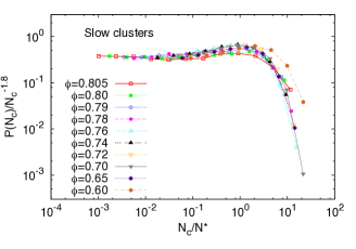
We now turn to the distribution of cluster sizes $P(N_{c})$ defined as the fraction of clusters of size $N_{c}$ (note that this is not the standard definition in percolation theory). In Fig. 12(a), $P(N_{c})$ for slow clusters is shown for $0.60\leq\phi\leq 0.805$. As the packing fraction increases, $P(N_{c})$ approaches a power law form $P(N_{c})\propto N_{c}^{-\kappa}$ up to a cutoff $N^{*}$ that grows with $\phi$. Fig. 13 shows $P(N_{c})/N_{c}^{-\kappa}$ as a function of $N_{c}/N^{*}$, where $N^{*}\propto(\phi_{c}-\phi)^{-1/\rho}$. Good collapse of the data is found for all packing fractions except the lowest one, with the following values for the fitting parameters: $\kappa\approx 1.8$ and $\rho\approx 1.63$. ($\phi_{c}=0.82$ was previously determined from the simultaneous fit of $\tau_{\alpha}$, $\chi_{4}$ and $\xi$). This suggests that the probability distribution has the scaling form

$$P(N_{c})\sim N_{c}^{-\kappa}f(N_{c}/N^{*})$$ (11)

and that $N^{*}\to\infty$ as $\phi\to\phi_{c}$ so that the distribution becomes a simple power law $P(N_{c})\propto{N_{c}}^{-\kappa}$.

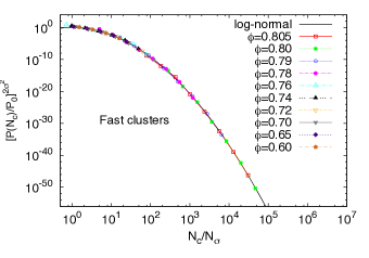
By contrast, $P(N_{c})$ for fast clusters, shown in Fig. 12(b), does not exhibit a power law behavior: there is clearly curvature in the log-log plot. However, a parabolic shape in the log-log plot corresponds to a log-normal distribution

$$P(N_{c})\propto N_{c}^{-1}\exp\{-[\ln(N_{c})-\ln(N_{0})]^{2}/(2\sigma^{2})\}\hskip 28.45274pt\mbox{.}$$ (12)

Rearranging Eq. (12), we obtain

$$\ln\{[P(N_{c})/P_{0}]^{2\sigma^{2}}\}=-[\ln(N_{c}/N_{\sigma})]^{2}\hskip 28.45274pt\mbox{,}$$ (13)

where $P_{0}$ is a normalization constant, and $N_{\sigma}=N_{0}\exp(-\sigma^{2})$. We have successfully fitted $P(N_{c})$ for each packing fraction to Eq. (13) where $P_{0}$, $N_{\sigma}$ and $\sigma$ are $\phi$-dependent fitting parameters. Fig. 14 shows a scaling plot of $[P(N_{c})/P_{0}]^{2\sigma^{2}}$ as a function of $N_{c}/N_{\sigma}$, where very good collapse is obtained for the data for all packing fractions. The log normal distribution for cluster sizes is the generic outcome of coalescence growth mechanisms ²⁹. It has been reported in various studies of elemental clusters, both metallic and non-metallic ^{29, 32, 30, 31}, but also in such dissimilar cases as the distribution of sizes of globular cluster systems in elliptical galaxies ³³.

3.4 Dynamic Susceptibility $\chi_{4}(t)$ and four-point structure function $S_{4}(q,t)$

$\chi_{4}(t)$ as a function of packing fraction

In the previous section we characterized spatial dynamic heterogeneities by directly analyzing the size and shape of slow and fast particles. A more common analysis of spatial dynamic heterogeneities is indirectly via four-point correlation functions ^{34, 35, 36}. We take this route in the following paragraph.

We begin with the dynamic susceptibility

$$\chi_{4}(t)=\overline{N[\left<Q^{2}_{\bf r}(t;t_{0})\right>-\left<Q_{\bf r}(t;t_{0})\right>^{2}]}.$$ (14)

This quantity gives a global measurement of the fluctuations, and can be interpreted as being proportional to the number of correlated slow particles.

Fig.  15: Dynamic susceptibility as defined in Eq. (14) as function of time $t$ for various $\phi$ (colors and symbols as in Fig. 3). Inset: $\tau_{4}$ against $\tau_{\alpha}$ for different packing fractions. The fit $\tau_{4}\propto\tau_{\alpha}^{1.19}$ excludes packing fractions $\phi>0.80$.

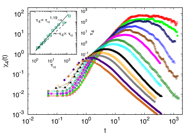
Fig. 15 shows $\chi_{4}(t)$ for various packing fractions $\phi$ with fixed $a=0.6$ ³⁷. The dominant features are a) a strong increase of the peak value, $\chi_{4}^{P}$, as $\phi_{c}$ is approached, indicating a strong increase in the number of correlated particles and b) a correspondingly strong increase of the time, $\tau_{4}$, when the peak occurs. The latter is in agreement with the slowing down of the dynamics, discussed in Sec. 3.1 for the dynamic overlap. In fact the time $\tau_{4}$ is related to the relaxation time $\tau_{\alpha}$ via a power law (see inset of Fig. 15). For the former, we had shown in ¹² that $\chi_{4}(\tau_{\alpha})\propto\left(\phi_{c}-\phi\right)^{-\gamma_{\chi}}$ with $\phi_{c}\approx 0.82$ and $\gamma_{\chi}\approx 2.5$.

Four-Point Structure Factor

The spatially resolved fluctuations of the overlap can be studied with the help of the four–point structure factor $S_{4}(q,t)$ given by

$$S_{4}(q,t)/N=$$

$$\left\{\overline{\left[\left\langle W_{\bf r}({\bf q},t;t_{0})W_{\bf r}({\bf-q},t;t_{0})\right\rangle-\left\langle W_{\bf r}({\bf q},t;t_{0})\right\rangle\left\langle W_{\bf r}(-{\bf q},t;t_{0})\right\rangle\right]}\right\},$$

where

$$W_{\bf r}({\bf q},t)=\frac{1}{N}\sum_{i=1}^{N_{\bf r}}\exp{[i{\bf q}\cdot{\bf r}_{i}(t_{0})]\theta(a-|{\bf r}_{i}(t_{0}+t)-{\bf r}_{i}(t_{0})|)}.$$ (16)

Here $\{{\cdots}\}$ denotes an average over wave vectors $\bf{q}$ of fixed magnitude $|{\bf q}|=q$.

Fig.  16: Four-point structure factor $S_{4}(q,\tau_{\alpha})$ for different packing fractions. The values at $q=0$ were obtained by the direct calculation of Eq. (3.4).

Fig.  17: Scaling plot of $S_{4}(q,\tau_{\alpha})$ for all simulated values of $\phi$ and $\varepsilon$ (see Sec. 3.4 below).

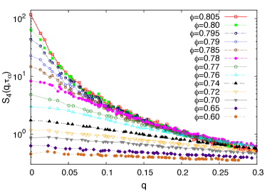
The four-point structure factor $S_{4}(q,\tau_{\alpha})$, evaluated at the $\alpha$-relaxation time, is displayed in Fig. 16 for various $\phi$. We observe a strong increase of $S_{4}(q,\tau_{\alpha})$ for small wavenumber as $\phi\to\phi_{c}$, which is to be expected since

$$\lim_{q\rightarrow 0}S_{4}(q,t)=\chi_{4}(t).$$ (17)

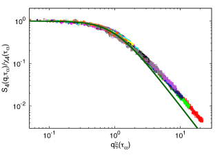
The data for all investigated packing fractions can be collapsed to a single curve, when plotting $S_{4}(q,\phi)/\chi_{4}(\phi)$ as a function of $q\xi(\phi)$, with all quantities evaluated at $t=\tau_{\alpha}$ (see Fig. 17). For small wavenumber the scaling function is well approximated by an Ornstein-Zernike (OZ) fit,

$$S_{4}(q,\tau_{\alpha})=\frac{\chi_{4}(\tau_{\alpha})}{1+[{q}\xi(\tau_{\alpha})]^{2}},$$ (18)

which allows us to extract the correlation length as a function of $\phi$. We had shown in ¹² that the resulting correlation length, $\xi(\tau_{\alpha})$, as function of $\phi$ diverges as a power law,

$$\xi(\tau_{\alpha})\propto\left(\phi_{c}-\phi\right)^{-\gamma_{\xi}},$$ (19)

with $\gamma_{\xi}=1.6$. Using a power law fit for $\tau_{\alpha}$ then implies an algebraic growth of the correlation length with relaxation time: $\tau_{\alpha}\propto\left[\xi(\tau_{\alpha})\right]^{z}$ where $z=\gamma_{\tau}/\gamma_{\xi}$. Such an algebraic dependence is in contrast to most 3D non–dissipative glasses where instead of an algebraic an exponential dependence prevails, but in agreement with a recent study ²³ of 2D glasses.

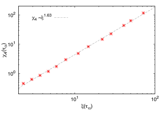
As already mentioned, $\chi_{4}(t)$ measures the number of particles moving together in a cooperative manner, and $\xi(t)$ is a measure for the spatial extension of these cooperative regions. Thus, from the relationship $\chi_{4}(t)\propto\xi^{d_{f}^{\prime}}(t)$ the exponent $d_{f}^{\prime}$ is usually interpreted as the fractal dimension of the clusters ². For instance, this would mean that the case of $d_{f}^{\prime}=d$ corresponds to compact clusters, whereas the case of $d_{f}^{\prime}=1$ corresponds to strings. The scaling behavior of $\chi_{4}(\tau_{\alpha})$ versus $\xi(\tau_{\alpha})$ for this system is shown in Fig. 18, with the fitted value $d_{f}^{\prime}\approx 1.6$. This is close to the value determined from the radius of gyration for $\phi\sim 0.6$, but fails to show the density dependence which we detected in Sec. 3.3. There we looked at clusters of a specific size, $N_{c}$, and determined their radius of gyration. Here the relation is less clear, because $\chi_{4}$ corresponds to an average or typical cluster size.

An alternative explanation for the observed scaling $\chi_{4}(t)\propto\xi^{d_{f}^{\prime}}(t)$ has been suggested, namely that correlated regions could be compact, but their sizes could have a wide distribution. The OZ form of $S_{4}(q,t)$ implies a sufficiently fast decay of $G_{4}(r,t)$ for large distances $r$ and hence is not compatible with a wide distribution on the largest scales. However, we have seen in Sec. 3.3 that the cluster size distribution indeed becomes increasingly wider as $\phi\to\phi_{c}$: The distribution decays algebraically, crossing over to an exponential at the cutoff $N^{*}$ which diverges as $\phi\to\phi_{c}$. Hence it becomes increasingly difficult to disentangle the two effects, namely the clusters compactifying and the distribution widening. Since the effects work in opposite directions, they might partially compensate. In any case the estimates of the fractal dimension directly from clusters of a specific size is superior to the rather indirect way using the relation between $\chi_{4}$ and $\xi$. The latter invariably gives rise to a constant value of $d_{f}^{\prime}$ as long as both quantities follow power laws with density independent exponents.

Fig.  18: $\chi_{4}(\tau_{\alpha})$ against $\xi(\tau_{\alpha})$. The dashed line corresponds to the fit $\chi_{4}(\tau_{\alpha})\propto\xi^{d_{f}^{\prime}}(\tau_{\alpha})$, with ${d_{f}^{\prime}}\approx 1.6$.

It is important to remark that, as demonstrated in Ref. ^{38, 39, 36}, the equivalence of $\chi_{4}(t)$ and the limit $S_{4}(q\to 0,t)$ is a subtle point. For numerical simulations where the particle density and the relative concentrations of each particle type are held fixed, additional contributions are required to relate the two quantities ^{39, 36}. In this work, since we cut the simulated box into sub–boxes of equal size, the number of particles and particle concentration varies with time and between sub–boxes. Therefore, all fluctuations are expected to be accounted for in Eq. (14), and no additional terms are needed in the calculation of $\chi_{4}(t)$. This means that the $q\rightarrow 0$ limit of $S_{4}(q,t)$ is expected to be well described by $\chi_{4}(t)$ obtained from the calculation of Eq. (14), whereas for other ensembles, $S_{4}(q=0,t)$ is obtained by an extrapolation of $\lim_{q\rightarrow 0}S_{4}(q,t)$ ^{40, 36} or by directly calculating the missing contribution to $\chi_{4}(t)$ as presented in Ref. ³⁶ (see Appendix).

Finite size analysis of $\chi_{4}$

It is clear from Eq. (14) that the dynamic susceptibility is a product of the variance of the overlap $Q_{\bf r}(t;t_{0})$, with a factor of $N$, which makes it scale like a constant as a function of $N$ in the thermodynamic limit $N\to\infty$.

The maximal value $\chi_{4}^{P}$ corresponds to a maximal number of correlated slow particles and is dependent on $\phi$ and the number of particles in the analyzed sub–box (see Sec. 2.1) as shown in Fig. 19(a). $\chi_{4}^{P}$ is observed to increase with system size as long as the system size is smaller than the correlation length and saturates once the system size is comparable or larger than the correlation length. These observations can be quantified using finite size scaling. The data for different $\phi$ can be collapsed approximately to a single function $\chi_{4}^{P}\xi^{\gamma_{\chi}/\gamma_{\xi}}(\sqrt{N}/\xi)$ as shown in Fig. 19(b) ⁴¹, where $\xi$, $\gamma_{\chi}$, and $\gamma_{\xi}$ were determined from $\chi_{4}$ and $S_{4}(q,t)$, as discussed above. Collapse of the data works well, in particular packing fractions $\phi\geq 0.76$ (see main panel of Fig. 19(b)), collapse in the full range $0.01<\sqrt{N}/\xi<100$. Data for lower packing fractions deviate from the scaling function, when the system size becomes comparable or larger than the correlation length (see inset of Fig. 19(b)). To conclude, finite size scaling of $\chi_{4}^{P}$ is fully consistent with the critical behavior extracted from $\chi_{4}(\tau_{\alpha})$ and $S_{4}(q,\tau_{\alpha})$.

Fig.  19: (a) Maximum value $\chi_{4}^{P}$ of the dynamic susceptibility as a function of the number of particles $N$ in the analyzed subbox. (b) Finite size scaling plot $\chi_{4}^{P}\xi^{\gamma_{\chi}/\gamma_{\xi}}(\sqrt{N}/\xi)$ with $\xi$, $\gamma_{\chi}$, and $\gamma_{\xi}$ as described in the text for packing fractions $\phi\geq 0.76$. Inset: Same quantities and axis range as in main panel for all packing fractions.

Cutoff Dependence

All previous results were calculated using $a=0.6$ (measured in units of $r_{1}$) in Eq. (5). This value has been chosen by most studies ^{40, 36, 42} which aim to calculate the extent of the dynamical heterogeneities and in particular $\xi(t)$. However, the dependence of the correlation length $\xi(t)$ on the parameter $a$ has not been explored in detail.

The growing behavior of $\xi(\tau_{\alpha})$ as a function of $a$ is shown in Fig. 20 for the range $0.2\leq a\leq 4.0$.

Fig.  20: $\xi({\tau_{\alpha}})$ against $a$ for $\phi=0.60$, $0.0.65$, $0.70$, $0.72$, $0.74$, $0.76$, $0.77$, $0.78$, $0.785$, $0.79$, $0.795$, $0.80$ and $0.805$ (from bottom to top). First, the grow of $\xi(\tau_{\alpha})$ occurs very rapidly for small $a$, then it goes through a crossover to finally go to a slower growth.

It can be observed that $\xi(\tau_{\alpha})$ goes through different regimes. First a rapid increase can be identified for $a\lesssim 1$, then, a crossover, and finally, a much slower growth for $a\gtrsim 1.2$.

In Fig. 21(a), we compare the correlation length as a function of $\phi$ for our standard choice ($a=0.6$) with two other choices of $a$, namely $a=1.4$ and $a=3.0$. All values for $\xi$ are obtained from the structure function $S_{4}(q,\tau_{\alpha})$ with help of a fit to the OZ form.

Fig.  21: (a) The dynamical correlation length $\xi(\tau_{\alpha})$ as a function of packing fraction $\phi$ for different values of the parameter $a$ of the overlap function. (b) $\chi_{4}(\tau_{\alpha})$ against $\xi(\tau_{\alpha})$ for three different choices of the parameter $a$. The different lines correspond to the fit $\chi_{4}(\tau_{\alpha})\propto\xi^{d_{f}^{\prime}}(\tau_{\alpha})$ for each $a$. We find similar fitted values of $d_{f}^{\prime}$ for the three different values of $a$.

In Fig. 21(a) a similar trend in the growing behavior of $\xi(\tau_{\alpha})$ with $\phi$ can be seen for the different values of $a$. Whereas for low packing fraction the points of $\xi(\tau_{\alpha})$ are very close to each other, the curves start to deviate considerably from each other for high packing fractions. This suggests that for the case of high packing fractions, when the heterogeneities in the dynamics become more pronounced, the selection of $a$ has a bigger impact on the result of $\xi$ than for low packing fractions, when the dynamics is governed by collisions between pairs of particles.

With this in mind, it should be interesting to determine how the relationship $\chi_{4}(\tau_{\alpha})\propto\xi^{d_{f}^{\prime}}(\tau_{\alpha})$ changes with different values of $a$. It turns out that despite the large difference in the values of $\xi$ for high packing fractions with the choice of $a$, the relationship $\chi_{4}(\tau_{\alpha})\propto\xi^{d_{f}^{\prime}}(\tau_{\alpha})$ only changes by a multiplicative constant, with the exponent $d_{f}^{\prime}$ similar for all values of $a$ mentioned before. These results are shown in Fig. 21(b) for the three different values of $a$. These results indicate that independently of the choice of $a$, $\chi_{4}(\tau_{\alpha})$ grows with $\xi(\tau_{\alpha})$ in the same way.

We also checked the fractal dimension obtained from the radius of gyration and again found it to be largely independent of $a$ in the range $0.6\leq a\leq 3$, for example for $\phi=0.76$, $1.78\lesssim d_{f}\lesssim 1.84$. This is slightly higher than the value found for $d_{f}^{\prime}$.

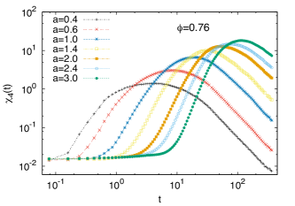
It is known that the height of the peak of $\chi_{4}(t)$ increases with increasing values of $a$ up to a certain value, which will be called $a_{\text{max}}$. Then, for $a>a_{\text{max}}$ the peak is seen to decrease ^{11, 40}. We do observe the expected increase of $\chi_{4}(t)$ for small $a$ (see Fig. 22) and the data indicate saturation around $a=3$. Also, we see the shift of $\chi_{4}(t)$ to longer times with increasing $a$. However, for the packing fractions studied in this work the value of $a_{\text{max}}$ was not reached. In order to reach this value, the simulations would have to be extended to much longer times. This is a difficult task considering the large number of collisions involved. We therefore leave this for future work.

Fig.  22: $\chi_{4}(\tau_{\alpha})$ for different values of the cutoff $a$.

Dependence on inelasticity $\varepsilon$

Different granular materials are characterized by different coefficients of restitution, determined by the microscopic properties of the constitutive grains. $\varepsilon$ is the control parameter which determines how non–dissipative a system is. Hence a question naturally arises: How universal are our results with respect to variations in $\varepsilon$? To answer this question, we present a few selected results:

The $\alpha$-relaxation time grows more slowly with packing fraction for the more inelastic system, indicating that $\phi_{c}$ increases with decreasing $\varepsilon$ (see Fig. 23), as predicted by mode-coupling theory ²⁰. From the point of view of the fits discussed in Sec. 3.1, this corresponds to the parameters $\phi_{c}(\varepsilon)$ and $\phi_{0}(\varepsilon)$ being monotonous decreasing functions of $\varepsilon$, as shown in the inset of Fig. 23.

Fig.  23: $\tau_{\alpha}$ as a function of $\phi$ for several values of $\varepsilon$; data fitted to $\tau_{\alpha}\propto(\phi_{c}-\phi)^{-\gamma_{\tau}}$ (dashed line for $\varepsilon=0.90$) and $\tau_{\alpha}\propto\exp{[B/(\phi_{0}-\phi)]}$ (solid line for $\varepsilon=0.90$); the resulting values of $\phi_{c}(\varepsilon)$ and $\phi_{0}(\varepsilon)$ are shown in the inset.

Similarly, the growing behavior of $\chi_{4}$ and $\xi$ is compatible with an $\varepsilon$–dependent critical density $\phi_{c}(\varepsilon)$ found in ²⁰ (not shown here). However, a robust scaling law relates the two quantities, $\chi_{4}(\tau_{\alpha})\propto\xi^{d_{f}^{\prime}}(\tau_{\alpha})$, with an exponent $d_{f}^{\prime}\sim 1.6$ which is independent of $\varepsilon$ (see Fig. 6 in ¹²).

The time-dependent overlap $Q(t)$ (Eq. (7)) for the range $0.7\leq\varepsilon\leq 1.0$ can equally well be fitted to the empirical form $Q^{-1}(t)=(t/\tau_{0})^{\beta}+1$. In fact the data in Fig. 6 include data sets for the above range of $\varepsilon$. Similarly, data for $S_{4}(q,t)$ for different values of $\varepsilon$ can be collapsed to the universal function shown in Fig. 17, in fact the data are included.

Fig.  24: Peak value of the dynamical susceptibility, $\chi_{4}^{P}$, versus $N$ for the packing fraction $\phi=0.78$ and coefficients of restitution $\varepsilon=1.0$, $0.90$, $0.80$, $0.70$. $\chi_{4}^{P}$ grows with $N$ before it saturates and it also grows as $\varepsilon$ is increased. Inset: the same data scaled as in Fig. 19(b).

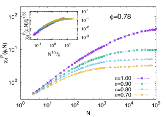
In Fig. 24 we present data for the peak value of $\chi_{4}^{P}$ as a function of $N$. For a given $\phi$, here $\phi=0.78$, the more inelastic systems are further away from criticality and hence $\chi_{4}(t)$ and $\xi$ are smaller. However the data can be collapsed with an $\varepsilon$-independent value of $d_{f}^{\prime}=1.58$.

All the scaling results described in this section show no significant difference between the elastic case $\varepsilon=1$ and the dissipative case $\varepsilon<1$. Therefore, we conclude that structural arrest occurs at higher packing fractions for the more inelastic systems but the main characteristics of dynamical heterogeneities are qualitatively the same for all investigated values of $\varepsilon$.

4 Conclusions

Via event driven simulations, we have investigated a two-dimensional homogeneously driven dissipative binary hard sphere system. All our results are consistent with a non-equilibrium glass transition which is controlled by the packing fraction, $\phi\to\phi_{c}$. Approaching this transition, we find long-lived and long-ranged dynamic heterogeneities which we have analyzed with several tools. Slow particles have been identified and analyzed in terms of a statistical distribution of cluster sizes. The latter obeys scaling and approaches an algebraic decay as $\phi\to\phi_{c}$, suggesting that macroscopically large clusters of slow particles exist in that limit. Similarly, clusters of fast particles can be identified. However, while the cluster size probability distributions for slow clusters have a behavior that is reminiscent of percolating systems near their critical point, the probability distributions for the sizes of fast clusters have a non-critical log-normal behavior. This suggests that any attempt at probing possible critical phenomena associated with the dynamical arrest should focus on the slow particles and not on the fast ones.

The spatial extent of the clusters has been characterized by the radius of gyration. Relating cluster size and spatial extent reveals a fractal dimension of the slow clusters which grows with $\phi$. In other words, the slow particles aggregate into progressively more compact clusters as $\phi\to\phi_{c}$.

Another route to studying dynamical heterogeneities is based on the overlap, defined as the fraction of particles which have moved less than a distance $a$ (usually $0.6$) in a given time interval t. The overlap itself shows pronounced slowing down as evidenced by a strong increase of the $\alpha$- relaxation time as $\phi\to\phi_{c}$. However, the time-dependent overlap does not obey time-density superposition, similar to results in Ref. ²³ for a 2D non–dissipative fluid. In contrast, Abate and Durian’s ¹¹ data for the overlap Q(t) for a 2D air-fluidized granular system seems to at least approximately satisfy time-density superposition (Fig. 3, top panel in ¹¹). All our data for different packing fractions and different coefficients of restitution can nevertheless be collapsed to a single curve with help of an empirical fit. The long-time decay is predicted to be algebraic in time.

Of particular interest are fluctuations of the overlap, – either global ones as measured by $\chi_{4}(t)$ or spatially resolved ones encoded in $S_{4}(q,t)$. The latter have been shown to obey scaling and are well approximated by the Ornstein–Zernike form. This allows us to extract a correlation length and the strength of the global fluctuations $\lim_{q\to 0}S_{4}(q,t)$. Since the latter have been computed independently, we can thereby show that $\chi_{4}(t)=\lim_{q\to 0}S_{4}(q,t)$. This result relies on our sub-box analysis mimicking a grand canonical ensemble with respect to particle number and concentration. The four point susceptibility was previously shown to diverge as $\chi_{4}(t)\propto(\phi_{c}-\phi)^{-\gamma_{\chi}}$, a result that we associate with a diverging number of correlated particles. Finite size scaling of $\chi_{4}(\phi,N)$ allows us furthermore to relate cluster size and correlation length. Using the previously determined values for $\xi$, we can collapse the data approximately to a single curve, providing a consistency check for the previously determined exponents $d_{f}^{\prime},\gamma_{\xi}$ and $\gamma_{\chi}.$

We have investigated the robustness of our results with respect to variations in the cutoff $a$ and the coefficient of restitution $\varepsilon$. The results suggest that the geometry of the clusters is largely insensitive to the definition of slow and fast particles and to the degree of inelasticity of the collisions between the particles. Even though $\chi_{4}$ and $\xi$ individually depend on $a$ and $\varepsilon$, the relation $\chi_{4}(\tau_{\alpha})\propto\xi^{d_{f}^{\prime}}(\tau_{\alpha})$ is surprisingly independent of those parameters.

Acknowledgments

We thank A. Fiege, I. Gholami and T. Kranz for help with the numerical simulations. H.E.C. thanks E. Flenner, and G. Szamel for discussions. This work was supported in part by DFG under grants SFB 602 and FOR 1394, by DOE under grant DE-FG02-06ER46300, by NSF under grants PHY99-07949 and PHY05-51164, and by Ohio University. K.E.A. acknowledges the CMSS program at Ohio University for partial support. K.V.L. thanks the Institute of Theoretical Physics, University of Göttingen, for hospitality and financial support.

Appendix

Fig.  25: Comparison of $\chi_{4}(\tau_{\alpha})$ obtained from Eq. (14), shown by the solid line, to $\chi_{0}$ obtained by fitting functions (2) and (3), shown as triangles and circles, respectively. In almost all cases the two values fall almost exactly on top of each other. The values of $\chi_{0}$ obtained from both fitting functions are very close to $\chi_{4}$.

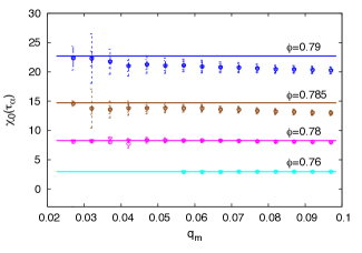
To check if the value of $\chi_{4}(\tau_{\alpha})$ can be obtained by an extrapolation of $S_{4}$ we determined $\chi_{0}(\tau_{\alpha})=\lim_{q\rightarrow 0}S_{4}(q,\tau_{\alpha})$ by allowing for more general fitting functions than just the OZ form:

$$S_{4}(q,\tau_{\alpha})=\frac{\chi_{0}}{1+({q}\xi)^{2}+A^{2}({q}\xi)^{4}}$$ (20)

suggested in ^{36, 43}. To confirm Eq. (17) we have determined $\chi_{0}(t)$ from two different fits of the above generalized expression for $S_{4}(q)$: in fit 2, $A=0$ and $\chi_{0}$ is a fit parameter and in fit 3, both $A$ and $\chi_{0}$ are fitted. The values obtained are shown as symbols in Fig. 25, and are compared to the value of $\chi_{4}(\tau_{\alpha})$ obtained form Eq. (14), shown as the solid line in the same figure. Furthermore we show in Fig. 25 the robustness of the fit with respect to the fitting range $[0:q_{m}]$. The agreement between $\chi_{0}(t)$ and $\chi_{4}(t)$ is remarkably good – for all packing fractions.

In addition, these different fits provide a check for the robustness of the extracted values of the correlation length. We found that different fitting functions did not change our results significantly. This holds for the whole range of packing fractions.