The Geometry of Sagittarius Stream from Pan-STARRS1 3 RR Lyrae
Abstract
We present a comprehensive and precise description of the Sagittarius (Sgr) stellar stream’s 3D geometry as traced by its old stellar population. This analysis draws on the sample of RR Lyrae (RRab) stars from the Pan-STARRS1 (PS1) 3 survey (Hernitschek et al., 2016; Sesar et al., 2017b), which is complete and pure within 80 kpc, and extends to kpc with a distance precision of . A projection of RR Lyrae stars within of the Sgr stream’s orbital plane reveals the morphology of both the leading and the trailing arms at very high contrast, across much of the sky. In particular, the map traces the stream near-contiguously through the distant apocenters. We fit a simple model for the mean distance and line-of-sight depth of the Sgr stream as a function of the orbital plane angle , along with a power-law background-model for the field stars. This modeling results in estimates of the mean stream distance precise to and it resolves the stream’s line-of-sight depth. These improved geometric constraints can serve as new constraints for dynamical stream models.
1 Introduction
Stellar streams around galaxies, and in particular around the Milky Way, are of great interest as their orbits are sensitive tracers of a galaxy’s formation history and gravitational potential (e.g. Eyre & Binney, 2009; Law & Majewski, 2010; Newberg et al., 2010; Sanders & Binney, 2013). In the Milky Way, the Sagittarius (Sgr) stream is the dominant tidal stellar stream of the Galactic stellar halo, and its extent has been traced around much of the sky. The stream shows two pronounced tidal tails extending each and reaching Galactocentric distances from 20 to more than 100 kpc, also referred to as “leading” and “trailing arm” (Majewski et al., 2003).
Stellar streams are sets of stars on similar orbits and therefore lend themselves to constraining the dynamical mass within their orbit. The distribution of Sgr stream’s stars can therefore serve as a probe of the Galactic mass profile and shape, including the dark matter halo. This is best done with 6-dimensional phase-space information available for the stars, as has been shown for relatively nearby streams such as GD-1 (Koposov et al., 2010; Bovy et al., 2016) and Ophiuchus (Sesar et al., 2016).
Since its discovery by Ibata et al. (1994), several work on sections of the Sagittarius stream was carried out. The first modeling attempt was done by Johnston et al. (1995), however, finding the progenitor, the Sagittarius dwarf galaxy, disrupting after only two orbits while observations show the completion of about 10 orbits. As a solution to the problem, Ibata & Lewis (1998) concluded from an extensive numerical study that the Sagittarius dwarf galaxy must have a stiff and extended dark matter halo if it has still about 25 % of its initial mass and is still bound today.
Early pencil-beam surveys before the large-scale survey era were used by Mateo et al. (1998), Martínez-Delgardo et al. (2001) and Martínez-Delgardo et al. (2004), reporting detections of tidal debris in the northern stream of the Sagittarius dwarf galaxy and leading to the publication of one of the first models of the Sagittarius stream being in good agreement with the observations (Martínez-Delgardo et al., 2004). Since the first detailed mapping by Majewski et al. (2003), there have been quite a number of attempts to map and trace the Sgr stream over larger fractions of its extent, at least in part e.g. building on the seminal work by Majewski et al. (2003). Such work was carried out by Niederste-Ostholt et al. (2010), who traced the Sgr stream out to kpc using main sequence, red giant, and horizontal branch stars from the SDSS as well as M giants from the Two Micron All-Sky Survey (2MASS), Koposov et al. (2012) who used main-sequence turn-off (MSTO) stars to measure the stream’s distance gradients between in the sourthern Galactic hemisphere, and Slater et al. (2013) using color-selected MSTO stars from the Pan-STARRS1 surved to present a panoramic view of the Sgr tidal stream in the southern Galactic hemisphere spanning .
Wide area surveys of the Galactic halo, employing RR Lyrae as tracers, have already been used in the past: Vivas et al. (2001) carried out a study on 148 RR Lyrae within the first 100 deg2 of the Quasar Equatorial Survey Team (QUEST) RR Lyrae survey, and after publishing a catalog (Vivas et al., 2004) continued using QUEST for finding substructure near the Virgo overdensity (Vivas et al., 2008). Duffau et al. (2014) (with Vivas) have extended the sample and found various velocity groups from QUEST and QUEST-La Silla (Zinn et al., 2014). Sesar et al. (2012) found two new halo velocity groups using RR Lyrae from the Palomar Transient Factory (PTF) survey, Sesar et al. (2013b) used a sample of 5000 RR Lyrae over 8000 deg2 of sky from the the Lincoln Near-Earth Asteroid Research asteroid survey (LINEAR) survey to analyze the Galactic stellar halo profile for heliocentric distances between 5 kpc and 30 kpc. Drake et al. (2014) produced a catalog of RR Lyrae and other periodic variables from the Catalina Surveys Data Release-1 (CSDR1).
A number of these attempts have been able to map parts of the Sagittarius stream. An extensive map was made by (Drake et al., 2013a, 2014), which confirms the presence of a halo structure that appears as part of the Sagittarius tidal stream, but is inconsistent with N-body simulations of that stream like the Law & Majewski (2010) model. Shortly before, this feature was confirmed by Belokurov et al. (2014) based on M-giants.
In more recent work, Belokurov et al. (2014) have demonstrated that the trailing arm of the Sgr stream can be traced out to its apocenter at kpc. They also give a fit of the stream’s leading arm to its apocenter at kpc. The extent of the Sgr stream has therefore only recently became fully apparent, spanning an unparalleled range of distances when compared to other stellar tidal streams in the Milky Way.
In contrast to the aforementioned partial mapping of the Sgr stream, showing the stream only piecewise mapped by tracers from different surveys and often relying on different kinds of sources as tracers, the data we have at hand – RR Lyrae stars from Pan-STARRS1 – enables us to trace the complete angular extent of the Sgr stream as well as to look even to the outskirts of the stream.
There have also been attempts to model the Sagittarius tidal stream (e.g. Law & Majewski, 2005; Peñarrubia et al., 2010; Gibbons et al., 2014), which has complex geometry and incomplete (so far) phase-space information.
Helmi (2004a) and Helmi (2004b) claim that the trailing arm is too young to be a probe of the dark matter profile, whileas the leading arm, being slightly older, provides a direct evidence for the prolate shape of the dark matter halo. Helmi (2004a) and Helmi (2004b) have used numerical simulations of the Sgr stream to probe the profile of the Milky Way’s dark matter halo. They find that the data available for the stream are consistent with a Galactic dark matter halo that could be either oblate or prolate, with minor-to-major density axis ratios can be as low as 0.6 within the region probed by the Sgr stream. In agreement with Martínez-Delgardo et al. (2004), they state that the dark matter halo should thus not be assumed as nearly spherical.
The modelling efforts have also included -body simulations constrained by observational data (e.g. Fellhauer et al., 2006; Law & Majewski, 2010; Peñarrubia et al., 2010; Dierickx & Loeb, 2017). Consistent 3D stream constraints from a single survey, as we set out to do here, aids the comparison to models of the Sgr stream, usually based on N-body simulation (e.g. Law & Majewski, 2010; Dierickx & Loeb, 2017).
The main aim of this paper is to map the geometry (in particular the distance) of the Sagittarius (Sgr) stream more precisely, accurately and comprehensively than before, using exclusively RR Lyrae stars (RRL) from a single survey to trace the stream’s old stellar population. For our analysis, we use the RRab sample of Sesar et al. (2017b), which covers of the sky, is rather pure and has precise distances (to ). It was generated from data of the Pan-STARRS1 survey (PS1) (Kaiser et al., 2010), using structure functions and a machine-learning algorithm by Hernitschek et al. (2016) and a subsequent multi-band light-curve fitting and another machine-learning algorithm as described in Sesar et al. (2017b).
This provides us with an RRL map of the old Galactic stellar halo that is of high enough contrast to fit the Sgr stream geometry directly by a density model: its distance and line-of-sigh-depth as a function of angle in its orbital plane. In particular, we can derive precise apocenter positions of both the leading and trailing arms and thus the Galactocentric orbital precession of the stream.
The structure of the paper is as follows: in Section 2 we describe
the PS1 survey and the RRL sample derived from it; in Section 3
we describe and apply the distance distribution model for the Sgr stream we fit to these
data; in Section 4 we present and discuss our results obtained from evaluating the fit, describe our findings regarding geometrical properties of the stream
and compare them to earlier work; we conclude with a discussion and summary in Section 5.
This work is part of a series of papers exploring the identification and astrophysical exploitation of RRL stars in the PS1 survey. The basic approach for applying multi-band structure functions to PS1 3 lightcurves, and subsequently using a classifier evaluating variability and color information to select RR Lyrae and QSO candidates has been laid out in Hernitschek et al. (2016), with results from the preliminary PS1 3 version, PV2. We then applied multi-band period fitting to all these RRL candidates (Sesar et al., 2017b), using light curves from the final PS1 3 version, PV3. The quality and plausibility of these fits aided in the classification, increasing the purity of the sample and leading to precise distance estimates for the sample of RRab stars. Sesar et al. (2017c) shows new detections within the Sgr stream, made using the RRab sample without further fitting or modeling; in particular, they show the detection of spatially distinct “spur” and clump features reaching out to more than 100 kpc on top of the apocenters of the Sgr stream, being in good agreement with recent dynamical models (Gibbons et al., 2014; Fardal et al., 2015; Dierickx & Loeb, 2017).
2 RR Lyrae Stars from the PS1 Survey
Our analysis is based on a sample of highly likely RRab stars, as selected by Sesar et al. (2017b) from the Pan-STARRS1 3 survey. In this section, we describe the pertinent properties of the PS1 3 survey and its obtained light curves, recapitulate briefly the process of selecting the likely RRab, as laid out in Sesar et al. (2017b); and we briefly characterize the obtained candidate sample.
The Pan-STARRS 1 (PS1) survey (Kaiser et al., 2010) is collecting multi-epoch, multi-color observations undertaking a number of surveys, among which the PS1 3 survey (Stubbs et al., 2010; Tonry et al., 2012; Chambers et al., 2016) is currently the largest. It has observed the entire sky north of declination in five filter bands () with a 5 single epoch depth of 22.0, 21.8, 21.5, 20.9 and 19.7 magnitudes in , and , respectively (Chambers et al., 2016).
For more than PS1 3 PV3 sources, we constructed a set of data features for source classification: the sources’ mean magnitudes in various bands, as well as multi-band variability features like a simple -related variability measure , and multi-band structure function parameters, , describing the characteristic variability amplitude and time-scale (Hernitschek et al., 2016). Based on these features, including a multi-band light-curve fit resulting in period estimates, a machine-learned classifier, trained on PS1 3 sources within SDSS S82, then selects plausible RRL candidates (Sesar et al., 2017b). Their distances were calculated based on a newly derived period-luminosity relation for the optical/near-infrared PS1 bands, as the majority of the PS1 sources lack metallicities. The complete methodology on how to derive the distances and verify their precision is given in Sesar et al. (2017b).
Overall, this highly effective identification of RR Lyrae stars has resulted in the widest (3/4 of the sky) and deepest (reaching kpc) sample of those stars to date. The RRab sample from Sesar et al. (2017b) were selected uniformly from the set of sources in the PS1 3 survey in the area and apparent magnitude range available for this survey. Sesar et al. (2017b) have shown that the selection completeness and purity for sources at high galactic latitudes () is approximately uniformly over a wide range of apparent magnitude up to a flux-averaged r-band magnitude of 20 mag, maintaining a sample completeness for the RRab stars of 80% and a purity of 90% within 80 kpc (see their Fig. 11).
We thus explicitly refer to high-latitude completeness on PS1 3 overlapping with SDSS Stripe 82 (Sesar et al., 2017b), but we have no reason to believe that the purity and completeness varies strongly across high-latitude areas. A detailed map of the purity and completeness including not only their distance but spatial distribution would require that we have “ground truth” (i.e.: knowledge about the true type of star for every source) in all directions, which is of course not available. For the definition of completeness and purity, we refer to Sesar et al. (2017b), where the completeness is defined as the fraction of recovered RR Lyrae stars on a test area (e.g. SDSS Stripe 82), and the purity is defined as the fraction of true RR Lyrae stars in the selected sample of RR Lyrae candidates.
There are 44,403 likely RRab stars in this PS1 sample with distance estimates that are precise to . In the further analysis, we refer to this sample (Hernitschek et al., 2016; Sesar et al., 2017b) as “RRab stars”.
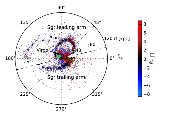
While the sample covers the entire sky above , we focus on stars near the Sgr stream orbital plane. We use the heliocentric Sagittarius coordinates as defined by Belokurov et al. (2014), where the equator is aligned with the plane of the stream. We restrict our subsequent analysis to RRab from our sample that lie within as also seen in the plots by Belokurov et al. (2014), resulting into stars. This sample is plotted in Fig. 1 in the plane of longitudinal coordinates and heliocentric distances , with the angular distance to the Sgr plane indicated by color-coding. A table for these stars within is given in the Appendix, Tab. 1. A machine readable version of this table is available in the electronic edition of the Journal.
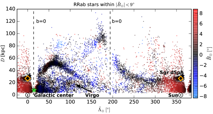
In this figure, the angular coordinate is running from to with repeated data points for and , to better show the distribution near .
The location of the Sun, Galactic anticenter, Sgr dSph and the Virgo overdensity (Vivas et al., 2001; Newberg et al., 2002; Jurić et al., 2008) are indicated. The dashed line marks the position of the Galactic plane. The centroid for Sgr dSph was taken from Karachentsev et al. (2004).
The Cetus stream should cross the Sgr stream at , (Newberg et al., 2009). From our data, every evidence is marginal.
3 A Simple Model to Characterize the Sgr Stream Geometry
We aim at a simple quantitative description of the Sgr stream, by providing the mean distance and line-of-sight (l.o.s.) depth of presumed member stars, as a function of angle in the orbital plane. We only consider stars within , and marginalize over their distribution perpendicular to the orbital plane, resulting in a set of distances as a function of . In practice, the overall distance distribution towards any is modeled as the superposition of a “stream” and “halo” component. At each bin, the halo is modeled as a power-law in Galactic coordinates, describing the background of field stars. The heliocentric distance distribution of stream stars is modeled as a Gaussian, characterized by and the l.o.s. depth, :
| (1) | |||||
where
| (2) |
with an analogous definition of . The data set is given as . The parameters are , composed of the fraction of the stars being in the Sgr stream at the given slice, the heliocentric distance of the stream , its l.o.s. depth , and the power-law index of the halo model. and are the minimum and maximum we consider in each slice.
We adopt a simple power-law halo model (Sesar et al., 2013b) to describe the “background” of field stars in the direction of :
| (3) |
with
Sesar et al. (2013b) also give the halo parameters
Here, is the number density of RR Lyrae at the position of the Sun, gives the halo flattening along the direction. In our analysis, all “background halo” parameters except the fitting parameter are kept fixed.
The stream is modeled as a normal distribution centered on and with variance as follows. It is defined in Galactic coordinates and Galactocentric distance , where is given as function of the heliocentric distances , , and distance uncertainty , as follows:
| (4) |
For the distance uncertainties of RRab stars, we adopt a of according to Sesar et al. (2017b).
3.1 Fitting the Sgr Model
For fitting this model, the sample of RRab stars near the Sgr orbital plane is split into bins of , each wide; the data are not binned in . In each bin, we fit (independently) the parameters of the stream, and , along with the halo model parameter . Whereas it is obvious why the stream-related model parameters should be fitted individually for each bin, the reason for fitting also the halo power law index individually is to account for incompleteness of the data. The flattening parameter is kept fixed at 0.71, as fitting for did not improve the results for the stream-related model parameters.
To constrain the geometry of the Sgr stream in a probabilistic manner, we calculate the joint posterior probability of the parameter set , given the data set . The marginal posterior probability of the parameter set , is related to the marginal likelihood through
| (5) |
where is the prior probability of the parameter value set.
We use the following prior probability for the model parameters, : for , we choose a prior that is uniform in , whereas for the other parameters, we adopt uniform priors. Specifically, we adopt
| (7) | ||||
The prior for depends on , and is uniform within , as indicated in Fig. 4 and listed in Tables 2 and 3. Whereas the prior is generally wide, a quite restrictive prior was chosen for and , as the fit otherwise behaves poorly because of the background sources along these lines of sight.
, are basically constrained by the minimum and maximum distance in the slice in case, but are also defined in order to mask dense regions at low heliocentric distances as well as to separate the leading and trailing arm where both are present at the same line of sight.
The most probable model given the data is explored using the Affine Invariant Markov Chain Monte Carlo (MCMC) ensemble sampler (Goodman & Weare, 2010) as implemented in the emcee package (Foreman et al., 2012).
The approach was verified with mock data, using a halo component that was sampled from the underlying halo model, superimposed by a mock stream that was inserted as a stellar density sheet; its number density is uniform perpendicular to the line of sight, and Gaussian along the line of sight. The fraction of the stream stars w.r.t. the halo stars, described by , was then successively lowered; i.e. the fit was carried out in the limit of many and few stars in each slice to make sure that reasonable fits can be obtained for densities like the ones present for the PS1 3 RR Lyrae candidates which is 0.5 – 1 deg-2 for most parts of the sky.
3.2 Fits to Individual Bins
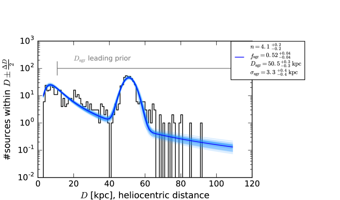
We now illustrate which practical issues are entailed in fitting the model to the data in a bin. Each distance and depth estimate is obtained by optimizing Equ. (6) using a MCMC (Foreman et al., 2012). Figures 2 and 3 show fits to individual slices in . Fig. 2 gives the fit for a wide slice centered on . In these direction, only the leading arm is present. The plot indicates the prior on , in these cases, only set by the minimum and maximum distance available from sources in the slice in case. The distribution of the sources is shown, overplotted with the model from the best-fit parameters given as a solid blue line. The transparent blue lines represent samples drawn from the parameter probability density function, illustrating the spread of models; the downturn of the models at small distances below kpc is also a reflection of our sample incompleteness (here at the bright end). In the case in Fig. 2, showing , a halo profile much steeper than expected from given in the Sesar et al. (2013b) model is obvious; local variations in presumably reflect simply the halo-substructure. The estimate of and is clearly seen as being sensible in Fig. 2. Here, the variance on the estimated parameters is very small, and the parameters fit well to what one would guess by visual inspection. Even for slices where the fit is poorer (both by visual inspection, and by the variance of the distance estimate) a sensible distance estimate, not driven by the priors, is found as we show below.
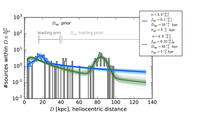
Fig. 3 gives the fit for , where both leading and trailing arms are along the line of sight. Using distinct priors on , separates both debris and gives precise estimates on distance and depth of both leading and trailing arm (see also Fig. 4 around ). This illustrates the importance of carefully set priors.
The source distance distribution is shown, overplotted with the model from the best-fit parameters given as solid blue line. The spread of transparent blue lines gives the spread of models obtained by the MCMC. The best-fit parameters are given along with their 1 uncertainties. The plot indicates the prior on , set by the minimum and maximum distance available from sources in this slice.
4 Results
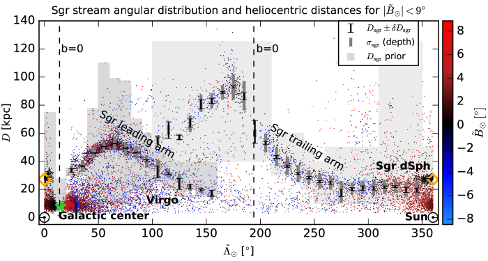
The modelling from Section 3 was then applied to the complete sample of RRab stars within . In Fig. 4, the resulting geometric characterization of the Sgr stream is shown, its fitted distance and line-of-sight (l.o.s) depth (actually ). It is apparent that the distance and l.o.s. depth estimates trace the stream well all the way out to more than 100 kpc. From this detailed picture of the Sgr stream, many features can be seen in great detail, some of them reported previously. The distances are shown as black points centered on the slice in case. Its l.o.s. depth is indicated by black bars. The grey shaded areas mark the priors set on ; clearly in most cases the priors play no significant role for the probability density function. The fitted parameter values are given in Tab. 4 and 5 in the Table Appendix.
Qualitatively the Sgr stream aspects shown in Figure 4 can be summarized as follows:
- (i)
-
(ii)
The leading arm’s apocenter lies between and where reaches kpc, and the trailing arm’s apocenter is near reaching its largest extent of 92.0 kpc. This agrees with Belokurov et al. (2014), who give the leading arm’s apocenter being located at and the trailing arm’s apocenter at . The precise position of the apocenters will be derived in Sec. 4.3.
-
(iii)
At both the apocenters of the main leading arm () and trailing arm () our RRab map reveals substructure that is readily apparent to the eye and has been more discussed in Sesar et al. (2017b) and Sesar et al. (2017c): two “clumps” (at and 80 kpc) beyond the leading arm’s apocenter, and a “spur” of the trailing arm reaching up to 130 kpc. Such features were previously predicted by dynamical models of the stream (e.g. Gibbons et al., 2014). These new Sgr stream features are discussed in Sesar et al. (2017b) in detail.
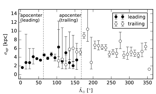
4.1 The Line-of-Sight Depth of the Sagittarius Stream
Fig. 5 shows the estimated of the stream (being half the l.o.s. depth) vs. for both the leading and trailing arm along with its uncertainty. Fig. 5 quantifies what was qualitatively apparent from Fig. 4(a): the stream tends to broaden along its orbit from 1.75 kpc to 6 kpc for the leading arm, reaching even 10 kpc for the trailing arm. As expected, and thus the l.o.s. depth is largest close to the apocenters. This is the first systematic determination of the l.o.s. depth, albeit the uncertainties are still quite large for some parts of the stream. The leading arm’s l.o.s. depth rises (and falls) towards (and away) from the apocenter. In contrast, for the trailing arm remains larger between . At least in part, this is presumably because our line-of-sight direction forms a shallower angle with the stream direction, compared to the leading arm. Except towards the apocenters, raises also towards the “end” (the largest ) of the respective trailing or leading arm.
In addition to the l.o.s. depth of the Sgr stream, the actual depth of the stream would be of great interest. As we know the angle between the normal on the stream, and the line of sight, we could deproject the l.o.s. depth to get the actual width of the stream.
First, we convert the polar coordinates of the projected , as shown in Fig. 4, into their Cartesian counterparts . We calculate then the deprojected depth for each bin in as
| (8) |
with
| (9) |
Equ. (9) approximates the tangent in with a line through and , thus the first and last of the leading and trailing arm are not deprojected.
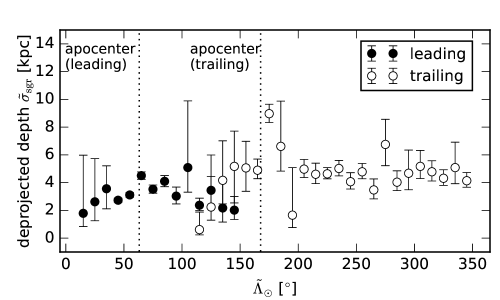
The deprojected depths along with their uncertainties are given in Tab. 6 and 7 in the Table Appendix. Fig. 6 shows how the l.o.s. and deprojected depth of the Sgr stream strongly varies during the orbital period. The profile is flatter than the profile, and as expected, the trailing arm’s deprojected depth is not noticeable boosted in contrast to which is. But a variation during the orbital period is still present. Comparing both depths emphasizes that the larger depth at the apocenters is a combination of the projection effect, as well as of the true broadening when the velocities become small near the apocenters.
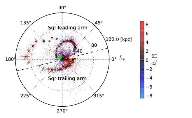
(a) Projection of the stream and its depth in cylindrical Sagittarius coordinates centered on the Sun. The orange bars indicate the deprojected depth, . The source distance distribution is shown with the same data, symbols and color coding as in Fig. 4.
(b) The deprojected depth of the Sagittarius stream from the RRab stars within of the Sagittarius plane. Error bars indicate the range. The general trend in the depth, seen in Fig. 5 for the l.o.s. depth , is still present here, but the profile is flatter than the profile from Fig. 5, as projection effects contribute to broadening near the apocenters. As in Fig. 5, the apocenter positions are indicated as dashed lines.
The deprojected depths along with their uncertainties are given in Tab. 6 and 7 in the Table Appendix.
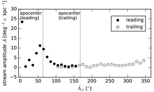
4.2 The Amplitude of the Sagittarius Stream
We can also quantify the amplitude of the stream fit from Sec. 3., defined as the number of RRab stars in the stream per degree as a function of , i.e.:
| (10) |
The amplitudes for both the leading and the trailing arm are given in Tab. 8 and 9 in the Table Appendix.
Fig. 7 shows the amplitudes plotted vs. the bins. The value of increases near the apocenter of the leading arm to about twice as much as away from its apocenter. Also near the apocenter of the trailing arm, rises w.r.t. the value it has away from the apocenter, but not as striking as found for the leading arm. As the angular velocity decreases near the apocenter, we had expected finding an increased source density, and thus larger , near the apocenters compared to sections of the stream away from apocenters. In addition to this general statement, we find that the source density is about six times larger at the leading arm’s than at the trailing arm’s apocenter (compare also Fig. 7 to Fig. 4). We checked if this can be partially explained by a selection effect, as the leading arm’s apocenter has a smaller heliocentric distance than the trailing arm’s. Using the selection function from Sesar et al. (2017b), we find that this will by far not account for the difference between the leanding and trailing arm’s apocenter source densities, so incompleteness is not an issue here. Additionally, simulations like Dierickx & Loeb (2017) also show a similar behavior, see e.g. Dierickx & Loeb (2017) Fig. 9 which shows a higher source density at the leading arm’s apocenter.
4.3 The Apocenters and Orbital Precession of the Sagittarius Stream
Sources orbiting in a potential show a precession of their orbits, which means that they do not follow an identical orbit each time, but actually trace out a shape made up of rotated orbits. This is because the major axis of each orbit is rotating gradually within the orbital plane.
Orbits in the outer regions of galaxies with a spherically symmetric gravitational potential are expected to have a precession between and (Belokurov et al., 2014). Assuming a spherically symmetric potential, the precession depends primarily on the shape of the potential and thus the radial mass distribution (Belokurov et al., 2014). Additionally it is also a function of the orbital energy and angular momentum distribution (Binney et al., 2008).
The angular mean distance estimates of the Sgr stream that were obtained during this work enable us to make statements about the precession of the orbit. For doing so, the angle between the leading and the trailing apocenters is measured.
We calculate this angle by fitting a model to the distance data in both the leading and trailing arm, namely fitting a Gaussian and a (shifted and scaled) log-normal. A comparable fit was carried out by Belokurov et al. (2014). The models used here are unphysical, but can be applied here as they describe the angular distance distribution adequately in order to find the apocenters along with their uncertainties. As the angular distance distribution of the leading arm appears to be symmetrical w.r.t. to the assumed apocenters, as well as appears to be Gaussian-like, a Gaussian model is fitted to the of the leading arm. In contrast, the trailing arm shows a clear asymmetry. fort this reason, we fit the trailing arm’s distance distribution using a (shifted an scaled) log-normal, fitted for the range . With comparable results, a parabola can be fitted to the data.
The best-fit Gaussian model for the leading and trailing apocenters, respectively, is shown in Fig. 8.
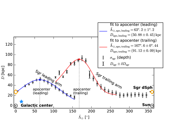
Blue and red lines show the best-fit models for both the leading and trailing arm. The position of the apocenters is denoted by a circle symbol in the corresponding color. Dashed lines mark the corresponding of each apocenter.
In this figure, blue and red lines show the best-fit Gaussian model for both the leading and trailing arm. The position of the apocenters is denoted by a circle symbol each. Dashed lines mark the apocenter’s corresponding .
We find the leading apocenter at , reaching , and the trailing apocenter at , reaching .
For a more detailed discussion of the apocenter substructure, reaching up to 120 kpc from the Sun, we refer to Sesar et al. (2017b), Section 3.
The differential orbit precession is , corresponding to a difference in heliocentric apocenter distances of kpc.
The actual Galactocentric orbital precession is slightly lower than the difference between the heliocentric apocenters. The Galactocentric distances and angles of the leading and trailing apocenters are calculated by taking into account the Galactocentric distance of the Sun being 8 kpc. Consequently, the opening angle between the positions of the two apocenters, as viewed from Galactic center, is then . The Galactocentric distance of the leading apocenter is then kpc, and of the trailing apocenter kpc, resulting into a difference in mean Galactocentric apocenter distances of kpc.
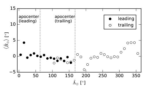
4.4 The Orbital Plane Precession of the Sagittarius Stream
Aside from the apocenter precession of the stream (see Sec. 4.3), the orbital plane itself might show a precession. To test this we obtain the weighted latitude of the stream RRab, , as a function of . The weight of each star is the probability that the star is associated with the Sgr stream.
For each bin in , the fit as described in Sec. 3.1 was carried out, resulting in a parameter set describing the stream and halo properties in the bin in case.
We now again make use of the model for the observed heliocentric distances, Equ. (1) with the halo described by Equ. (3) and the stream described by Equ. (4). We calculate as the fraction of the likelihood a star is associated with the Sgr stream divided by the sum of the likelihood that it is associated with Sgr stream and the likelihood that the star is associated with the halo:
| (11) |
The weighted latitude in a bin is then calculated as
| (12) |
We then use the difference in for the leading and trailing arm to quantify the orbital plane precession.
The resulting for both the leading and the trailing arm are given in Tab. 8 and 9 in the Table Appendix. Fig. 9 shows plotted vs. the bins.
This gives evidence for the leading arm staying in or close to the plane defined by , whereas the trailing arm is found within within to around the plane. From this, we find a separation of , as also derived by Law et al. (2005).
5 Discussion
We can now put our results in the context of existing work, and discuss the prospect of using them for dynamical stream modeling.
5.1 Comparison to the Model by Belokurov et al. (2014)
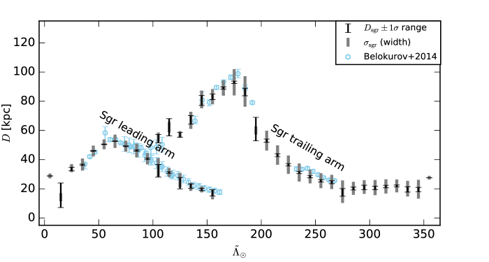
The best previous estimates of the heliocentric distances for a large part of the Sgr stream come from Belokurov et al. (2014), who used blue horizontal branch (BHB) stars, sub-giant branch (SGB) stars and red giant branch (RGB) stars from the Sloan Digital Sky Survey Data Release 8 (SDSS DR8). In Fig. 10 we compare our heliocentric distances, to those from Belokurov et al. (2014) (Figure 6 therein). We show the uncertainties from Belokurov et al. (2014) where available, and assume the uncertainties to be if not stated otherwise.
Overall, the two estimates are in good agreement, attesting to the quality of the Belokurov et al. (2014) analysis. The distances from Belokurov et al. (2014) may be systematically slightly larger; the fact that the RRab distances we use are directly tied to HST and Gaia DR1 parallaxes (Sesar et al., 2017b) should lend confidence to the distance scale of this work. Our new estimates for the mean distance are three times more precise, and presumably also accurate. The typical mean distance uncertainty in Belokurov et al. (2014) is kpc and up to 0.1 for most parts of the stream, whereas our work shows comparable or smaller (see Tables 4, 5).
As mentioned before, our new Sgr stream map also has considerably more extensive angular coverage.
The high individual distance precision to the RRab of allows us to map the l.o.s. depth of the stream, which Belokurov et al. (2014) could not do, or at least did not. For these reasons, our work improves the knowledge on the geometry of Sgr stream significantly.
However, care must be taken in parts of the Sgr stream where the number of sources is comparably low. The trailing arm’s distance estimate for the bin centered on results from only 28 sources within the prior indicated by Fig. 4(a), i.e. kpc. In this bin, the estimated is smaller than the estimated for nearby bins, and the same applies for the estimated width of the stream which appears being too tight.
In both analyses, the apocenters of the leading and trailing arms are derived.
We find the leading apocenter at , reaching , and the trailing apocenter at , reaching . The differential orbit precession is , with a difference in heliocentric apocenter distances of kpc. Taking into account the Galactocentric distance of the Sun being 8 kpc, the corresponding Galactocentric angle from our analysis is . The Galactocentric distance of the leading apocenter is then kpc, and of the trailing apocenter kpc, resulting into a difference in mean Galactocentric apocenter distances of kpc.
If we would assume the trailing arm’s apocenter is close to the maximum extent of the derived , as done by fitting a Gaussian to the five closest points near the maximum extent, we find trailing apocenter at , reaching . The differential orbit precession is then , with a difference in heliocentric apocenter distances of kpc. The Galactocentric angle is then slightly larger than for the log-normal fit, , the Galactocentric distance of the leading apocenter kpc, to the trailing apocenter kpc, resulting into a difference in mean Galactocentric apocenter distances of kpc.
Belokurov et al. (2014) give the position of the leading apocenter as with a Galactocentric distance kpc, and the position of the trailing apocenter as with a Galactocentric distance kpc. They state the derived Galactocentric orbital precession as .
To summarize the comparison:
-
•
Our analysis is done from one single survey and type of stars, whereas the work by Belokurov et al. (2014) relies on BHB, SGB and RGB stars. The extent and depth of PS1 3 enables us to provide a more extensive angular coverage of sources. This resulted into the first complete (i.e., spanning ) trace of Sgr stream’s heliocentric distance from a single type of stars originating from a single survey.
- •
-
•
Along with the extent of the Sgr stream, we can give its l.o.s. depth , and deproject in order to get its true width.
-
•
Our analysis shows a Galactocentric orbital precession being about larger than as measured by Belokurov et al. (2014), or larger if assuming the trailing arm’s apocenter is close to the maximum extent of the derived . This is within the error range given by Belokurov et al. (2014). Generally speaking, the higher the Galactocentric orbital precession, the smoother the dark matter densitiy is as a function of the Galactocentric radius. Logarithmic haloes should show an orbital precession of about (Belokurov et al., 2014), whereas a smaller orbital precession angle indicats a profile with a sharper drop in the radial dark matter density (Belokurov et al., 2014). Finding this result, together with the result of (Belokurov et al., 2014) as well as the simulation by Dierickx & Loeb (2017) is a strong indicator that a steeper profile than the logarithmic one should be considered for the dark matter halo of the Milky Way.
Uncertainties from our results are given as ranges; uncertainties from Belokurov et al. (2014) are given as their ranges if available, and assumed to be if not stated otherwise.
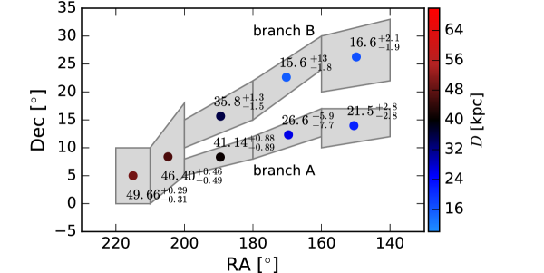
5.2 Bifurcation of the Leading Arm
Part of the Sgr stream’s leading arm in the Galactic Norther hemisphere is “bifurcated”,
or branched, in its projection on the sky (Belokurov et al., 2006). Starting at , the lower and upper declination branches of the stream, labeled A and B respectively (Belokurov et al., 2006), can be traced at least until . As stated by Fellhauer et al. (2006), the bifurcation likely arises from different stripping epochs, the young leading arm providing branch A and the old trailing arm branch B of the bifurcation.
Belokurov et al. (2006) states that the SGB of branch B is significantly brighter and hence probably slightly closer than A, but the branch itself is reported to have much lower luminosity compared to A.
Their Fig. 4 shows a noticeable, but small difference in the distances estimated for branches A and B of 3 to kpc, qualitatively consistent with the simulations by Fellhauer et al. (2006). However, Ruhland et al. (2011) found from an analysis of BHB stars in the stream that the branches differ by at most 2 kpc in distance. To follow up on this, we measured the RRab mean distances for small patches in both branches, as shown by the polygons in Fig. 11, fitting a halo and stream model as described above in Section 3. This fitting led to the distance estimates as shown in Fig. 11 and in Tab. 10 in the Table Appendix. Indeed a small distance difference between the two branches can be found, branch B being closer than branch A like in the simulation by Fellhauer et al. (2006). But the sparse sampling by the RR Lyrae makes this analysis inconclusive.
5.3 Bifurcation of the Trailing Arm
Analogous to the bifurcation of the leading arm found by Belokurov et al. (2006), Koposov et al. (2012) found a similar bifurcation in the Sgr stream trailing arm, consisting of two branches that are separated on the sky by .
These bifurcation was later confirmed and studied in greater detail by Slater et al. (2013), using main-sequence turn-off (MSTO) and red clump (RC) stars from the Pan-STARRS1 survey, and Navarrete et al. (2017), who have examined a large portion of approximately of the Sgr trailing arm available in the imaging data from the VST ATLAS survey, using BHB and SGB stars, as well as RR Lyrae from CRTS.
They found the trailing arm appearing to be split along the line-of-sight, with the additional stream component following a distinct distance track, and a difference in heliocentric distances exists of kpc. The bulk of the “bright stream” (Slater et al., 2013) is below the Sgr orbital plane (thus ), while the “faint stream” lies mostly above the plane ( ).
We compare here our distance distributions to the findings of Slater et al. (2013) and Navarrete et al. (2017) for different regions in .
Navarrete et al. (2017) report a bifurcation in the plane with a separation of . Likely due to our relatively sparse source density, we can not find an indicator for a bifurcation in the plane that would lead to a “bright stream” and “faint stream”.
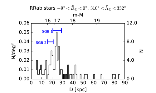
We then checked whether we can identify l.o.s. substructures, and made histograms of the heliocentric distance distribution for several patches along the trailing arm of the Sgr stream.
In Fig. 12, we give a histogram of our distance estimates in one of the regions probed by Navarrete et al. (2017) and Slater et al. (2013). This specific region was also probed using RR Lyrae by Navarrete et al. (2017) (see their Fig. 9). We give our estimates of the heliocentric distance and the distance modulus (Sesar et al., 2017b). Blue markers represent substructures found by Navarrete et al. (2017). A similar shape of the distance distribution is found, and we also detect the substructures they call “SGB 1” and “SGB 2”. We find “SGB 1” at a slightly larger distance than Navarrete et al. (2017). We find “SGB 2” split into two components.
We were also able to identify similar substructures as found by Navarrete et al. (2017) and Slater et al. (2013) within other patches of the Sgr stream trailing arm, and count them as tentative but marginal significant because the relatively low density of our tracers.
6 Summary
In this work, we quantified the geometry of the Sagittarius stream, characterizing the l.o.s. density of the Sagittarius stream approximated by a Gaussian distribution centered on the distance , having the l.o.s. depth . This model was used to estimate distance and depth of the Sgr stream as given by RR Lyrae candidates (RRab with completeness 0.8, purity=0.9 up to 80 kpc, distance precision of ) resulting from the classification that incorporates period fitting.
The fitting resulted into the best and first basically complete (i.e., spanning ) trace of Sgr stream’s heliocentric distance, as well as l.o.s. depth. This model allows further to measure many properties of the Sgr stream. We have measured the depth as well as the deprojected depth of the stream. The function of vs. can be partially explained by projection effects, and partially by projection effects due to the angle our line-of-sight direction forms with the stream direction.
Deprojection removes the line-of-sight effects and thus results into a depth of the stream that will be very helpful when comparing simulations to observational data.
Further on, we computed the amplitude of the Str stream as the number of RRab stars in the sream per degree as a function of its longitude .
The fit allows us to precisely determine the apocenter positions, from which we then calculate the orbital precession. We also find a strong indicator for a precession of the orbital plane.
We have measured the Galactocentric angle between the apocenters of the leading and trailing arm of the Sgr stream and the difference between their respective distances.
Having now a model of the geometry of the Sgr stream at hand, it can be used to further constrain the Milky Way’s potential.
Appendix A Tables
Table 1 gives the PS1 RRab stars with this analysis is based on.
Tables 2 and 3 give the minimum and maximum prior on , and , as indicated in Fig. 4. The annotation “max” within the tables state that the given value is the maximum observed heliocentric distance in the given interval.
Tables 4 and 5 give the geometry of the Sagittarius stream, represented by its extent and depth as inferred from the analysis presented in this paper.
Tables 8 and 9 give the amplitude of the Sagittarius stream. as well as the weighted latitude of the stream, as calculated by Equ. (12).
Table 10 gives the distance estimates for the branches A and B of the Sagittarius stream.
| RA | Dec | DMb | Period | |||
|---|---|---|---|---|---|---|
| (deg) | (deg) | (mag) | (day) | (day) | (mag) | |
| 181.40332 | 7.77677 | 1.00 | 17.08 | 0.6752982619 | 0.24526 | 0.75 |
| 181.12043 | 8.28025 | 0.91 | 12.79 | 0.5382632283 | 0.44801 | 0.63 |
| 180.08748 | 9.10501 | 1.00 | 17.76 | 0.5203340425 | -0.46188 | 0.88 |
Note. — A machine readable version of this table is available in the electronic edition of the Journal. A portion is shown here for guidance regarding its form and content.
| interval (deg) | (kpc) | (kpc) |
|---|---|---|
| 5 | 27.3 (max) | |
| 30 | 35 | |
| 30 | 37 | |
| 10 | 77.5 (max) | |
| 10 | 110.1 (max) | |
| 10 | 98.9 (max) | |
| 10 | 97.2 (max) | |
| 20 | 70 | |
| 20 | 60 | |
| 25 | 50 | |
| 20 | 50 | |
| 15 | 40 | |
| 20 | 40 | |
| 15 | 40 | |
| 15 | 40 |
| interval (deg) | (kpc) | (kpc) |
|---|---|---|
| 50 | 95.1 (max) | |
| 50 | 98.9 (max) | |
| 40 | 92.6 (max) | |
| 10 | 92.7 (max) | |
| 40 | 106.0 (max) | |
| 40 | 134.2 (max) | |
| 10 | 125.1 (max) | |
| 10 | 131.7 (max) | |
| 10 | 103.6 (max) | |
| 10 | 72.6 (max) | |
| 40 | 73.8 (max) | |
| 10 | 64.6 (max) | |
| 30 | 60 | |
| 30 | 60 | |
| 20 | 50 | |
| 10 | 40 | |
| 10 | 50 | |
| 10 | 50 | |
| 10 | 50 | |
| 10 | 50 | |
| 10 | 50 | |
| 10 | 80.0 (max) | |
| 10 | 84.7 (max) | |
| 10 | 64.6 (max) | |
| 10 | 86.4 (max) | |
| 10 | 50.0 |
| (deg) | a | (kpc)b | (kpc)c | ||||||||
|---|---|---|---|---|---|---|---|---|---|---|---|
| 5 | 0.18 | 28.830 | 0.10 | 0.094 | 0.20 | 0.18 | 1.621 | 0.079 | 0.091 | 0.15 | 0.18 |
| 15 | 0.052 | 14.3 | 7.1 | 9.7 | 9.1 | 12.0 | 2.8 | 1.5 | 6.5 | 1.7 | 15 |
| 25 | 0.050 | 34.14 | 1.8 | 0.66 | 3.8 | 0.83 | 2.8 | 1.4 | 3.3 | 1.7 | 9.3 |
| 35 | 0.051 | 36.65 | 0.60 | 0.27 | 1.9 | 0.34 | 4.1 | 1.7 | 1.9 | 2.9 | 4.6 |
| 45 | 0.38 | 45.94 | 0.24 | 0.25 | 0.48 | 0.52 | 3.68 | 0.19 | 0.20 | 0.36 | 0.43 |
| 55 | 0.51 | 50.50 | 0.17 | 0.17 | 0.34 | 0.33 | 3.33 | 0.18 | 0.18 | 0.34 | 0.38 |
| 65 | 0.61 | 52.59 | 0.21 | 0.21 | 0.43 | 0.44 | 4.52 | 0.27 | 0.27 | 0.54 | 0.53 |
| 75 | 0.41 | 49.19 | 0.26 | 0.27 | 0.52 | 0.53 | 3.75 | 0.30 | 0.33 | 0.57 | 0.72 |
| 85 | 0.36 | 46.22 | 0.40 | 0.39 | 0.83 | 0.78 | 4.66 | 0.44 | 0.47 | 0.79 | 0.99 |
| 95 | 0.21 | 40.59 | 0.48 | 0.53 | 0.95 | 1.1 | 3.88 | 0.72 | 0.83 | 1.3 | 1.9 |
| 105 | 0.26 | 34.8 | 6.7 | 1.9 | 9.4 | 2.8 | 6.3 | 2.2 | 6.0 | 3.2 | 8.8 |
| 115 | 0.22 | 31.19 | 0.57 | 0.54 | 1.3 | 1.0 | 3.08 | 0.51 | 0.66 | 0.91 | 1.7 |
| 125 | 0.25 | 25.9 | 5.9 | 1.9 | 9.9 | 3.0 | 5.0 | 1.9 | 3.7 | 2.8 | 6.2 |
| 135 | 0.067 | 21.34 | 0.92 | 2.1 | 1.3 | 8.9 | 2.7 | 1.3 | 2.7 | 1.7 | 6.5 |
| 145 | 0.13 | 19.66 | 0.87 | 0.80 | 2.2 | 20.0 | 2.05 | 0.68 | 1.0 | 0.99 | 2.5 |
| 155 | 0.15 | 16.2 | 1.1 | 3.2 | 1.1 | 3.2 | 3.4 | 2.2 | 2.6 | 2.2 | 2.6 |
| (deg) | a | (kpc)b | (kpc)c | ||||||||
|---|---|---|---|---|---|---|---|---|---|---|---|
| 105 | 0.055 | 55.4 | 3.9 | 1.9 | 5.2 | 3.5 | 3.2 | 1.5 | 7.2 | 2.0 | 13 |
| 115 | 0.056 | 62.3 | 6.0 | 5.8 | 11 | 10 | 3.5 | 2.2 | 7.3 | 2.5 | 14 |
| 125 | 0.059 | 57.2 | 1.9 | 1.4 | 11 | 11 | 2.3 | 0.97 | 2.2 | 1.3 | 12 |
| 135 | 0.084 | 66.9 | 2.6 | 3.2 | 5.0 | 7.2 | 5.8 | 2.4 | 4.0 | 4.1 | 9.9 |
| 145 | 0.095 | 81.3 | 4.1 | 2.7 | 8.7 | 4.4 | 6.1 | 3.1 | 3.0 | 4.6 | 6.2 |
| 155 | 0.31 | 83.1 | 1.9 | 1.8 | 1.9 | 1.8 | 5.2 | 1.7 | 3.0 | 1.7 | 2.0 |
| 165 | 0.36 | 89.02 | 0.72 | 0.74 | 1.5 | 1.5 | 5.13 | 0.64 | 0.85 | 1.2 | 2.0 |
| 175 | 0.63 | 92.98 | 0.79 | 0.81 | 1.6 | 1.6 | 8.99 | 0.64 | 0.68 | 1.3 | 1.4 |
| 185 | 0.40 | 86.7 | 3.0 | 2.2 | 7.0 | 4.6 | 10.5 | 2.8 | 5.2 | 4.6 | 8.7 |
| 195 | 0.082 | 60.0 | 7.1 | 9.0 | 17 | 12 | 2.8 | 1.5 | 5.8 | 1.8 | 15 |
| 205 | 0.55 | 53.0 | 1.2 | 1.1 | 2.6 | 2.1 | 6.78 | 0.82 | 0.95 | 1.5 | 2.2 |
| 215 | 0.61 | 43.15 | 1.1 | 0.88 | 2.4 | 1.8 | 6.65 | 0.97 | 1.2 | 1.8 | 2.4 |
| 225 | 0.71 | 36.55 | 0.87 | 0.75 | 1.8 | 1.4 | 6.28 | 0.49 | 0.61 | 0.97 | 1.4 |
| 235 | 0.55 | 31.17 | 0.70 | 0.80 | 1.1 | 1.6 | 6.16 | 0.65 | 0.71 | 1.3 | 1.5 |
| 245 | 0.58 | 28.41 | 0.85 | 0.69 | 1.9 | 1.3 | 4.66 | 0.60 | 0.75 | 1.1 | 1.7 |
| 255 | 0.62 | 25.57 | 0.85 | 0.72 | 1.9 | 1.4 | 5.14 | 0.54 | 0.64 | 1.0 | 1.4 |
| 265 | 0.43 | 24.7 | 1.2 | 0.87 | 2.8 | 1.6 | 4.86 | 0.90 | 1.1 | 1.7 | 2.4 |
| 275 | 0.60 | 18.0 | 3.1 | 2.1 | 7.0 | 3.9 | 7.7 | 1.8 | 2.1 | 3.3 | 4.2 |
| 285 | 0.32 | 20.34 | 1.1 | 0.83 | 2.7 | 1.6 | 4.44 | 0.67 | 0.90 | 1.2 | 2.2 |
| 295 | 0.27 | 21.2 | 1.8 | 1.2 | 5.4 | 2.2 | 4.7 | 1.2 | 1.7 | 2.0 | 4.2 |
| 305 | 0.37 | 20.8 | 1.3 | 1.0 | 3.4 | 1.9 | 5.17 | 0.88 | 1.1 | 1.6 | 2.8 |
| 315 | 0.45 | 21.66 | 0.95 | 0.80 | 2.0 | 1.5 | 4.84 | 0.67 | 0.80 | 1.3 | 1.8 |
| 325 | 0.48 | 22.00 | 0.75 | 0.62 | 1.7 | 1.2 | 4.41 | 0.52 | 0.63 | 0.97 | 1.5 |
| 335 | 0.40 | 20.1 | 2.3 | 1.4 | 7.3 | 2.3 | 5.3 | 1.2 | 1.9 | 2.1 | 4.6 |
| 345 | 0.47 | 19.7 | 1.7 | 1.3 | 4.7 | 2.4 | 6.43 | 0.73 | 0.92 | 1.4 | 2.3 |
| 355 | 0.43 | 27.605 | 0.054 | 0.053 | 0.11 | 0.11 | 1.245 | 0.048 | 0.047 | 0.091 | 0.096 |
| (deg) | |||
|---|---|---|---|
| 15 | 1.79 | 0.83 | 6.0 |
| 25 | 2.6 | 1.3 | 5.7 |
| 35 | 3.6 | 2.1 | 5.2 |
| 45 | 2.7 | 2.6 | 2.9 |
| 55 | 3.1 | 2.9 | 3.3 |
| 65 | 4.5 | 4.2 | 4.8 |
| 75 | 3.5 | 3.2 | 3.8 |
| 85 | 4.1 | 3.7 | 4.5 |
| 95 | 3.0 | 2.5 | 3.7 |
| 105 | 5.1 | 3.3 | 9.9 |
| 115 | 2.4 | 2.0 | 2.9 |
| 125 | 3.4 | 2.2 | 6.0 |
| 135 | 2.2 | 1.2 | 4.3 |
| 145 | 1.7 | 1.2 | 2.6 |
| (deg) | |||
|---|---|---|---|
| 115 | 0.61 | 0.24 | 1.9 |
| 125 | 2.2 | 1.3 | 4.4 |
| 135 | 4.2 | 2.5 | 7.0 |
| 145 | 5.2 | 2.5 | 7.7 |
| 155 | 5.1 | 3.4 | 7.0 |
| 165 | 4.9 | 4.3 | 5.7 |
| 175 | 9.0 | 8.3 | 9.6 |
| 185 | 6.6 | 4.8 | 9.9 |
| 195 | 1.65 | 0.76 | 5.1 |
| 205 | 5.0 | 4.4 | 5.7 |
| 215 | 4.6 | 3.9 | 5.4 |
| 225 | 4.6 | 4.3 | 5.1 |
| 235 | 5.0 | 4.5 | 5.6 |
| 245 | 4.1 | 3.5 | 4.7 |
| 255 | 4.8 | 4.3 | 5.4 |
| 265 | 3.5 | 2.8 | 4.3 |
| 275 | 6.8 | 5.2 | 8.6 |
| 285 | 4.0 | 3.4 | 4.9 |
| 295 | 4.7 | 3.5 | 6.3 |
| 305 | 5.2 | 4.3 | 6.3 |
| 315 | 4.8 | 4.1 | 5.6 |
| 325 | 4.3 | 3.8 | 4.9 |
| 335 | 5.1 | 3.9 | 6.9 |
| 345 | 4.1 | 3.7 | 4.7 |
| (deg) | (deg kpc-1) | (deg) |
|---|---|---|
| 5 | 24 | 0.48 |
| 15 | 0.53 | 4.3 |
| 25 | 3.9 | -0.41 |
| 35 | 1.2 | 0.40 |
| 45 | 7.4 | 0.90 |
| 55 | 11 | 0.14 |
| 65 | 9.5 | -0.11 |
| 75 | 5.4 | 0.39 |
| 85 | 3.0 | -0.67 |
| 95 | 1.9 | -0.47 |
| 105 | 1.1 | -0.74 |
| 115 | 1.5 | -1.4 |
| 125 | 0.70 | -0.65 |
| 135 | 0.44 | -1.4 |
| 145 | 1.0 | -0.25 |
| 155 | 0.62 | -2.0 |
| (deg) | (deg kpc-1) | (deg) |
|---|---|---|
| 105 | 0.47 | -2.1 |
| 115 | 0.33 | -0.51 |
| 125 | 0.37 | -0.96 |
| 135 | 0.26 | -1.5 |
| 145 | 0.25 | -2.0 |
| 155 | 0.85 | -1.8 |
| 165 | 1.2 | -1.2 |
| 175 | 1.6 | 0.59 |
| 185 | 0.46 | -0.18 |
| 195 | 0.067 | -4.2 |
| 205 | 0.93 | -2.6 |
| 215 | 1.2 | -0.60 |
| 225 | 1.8 | -0.15 |
| 235 | 1.2 | -0.34 |
| 245 | 1.6 | 0.91 |
| 255 | 1.6 | 0.55 |
| 265 | 1.2 | -0.12 |
| 275 | 1.1 | -0.48 |
| 285 | 1.1 | -0.08 |
| 295 | 1.3 | -0.20 |
| 305 | 1.6 | 1.3 |
| 315 | 1.8 | 2.4 |
| 325 | 3.1 | 4.2 |
| 335 | 2.3 | 4.3 |
| 345 | 3.6 | 4.3 |
| 355 | 54 | 0.88 |
| RA (deg) a | Dec (deg) a | b | (kpc)c | (kpc)c | ||||||||
|---|---|---|---|---|---|---|---|---|---|---|---|---|
| 215 | 5 | 0.49 | 49.77 | 0.31 | 0.32 | 0.63 | 0.66 | 3.18 | 0.43 | 0.52 | 0.83 | 1.1 |
| 204.783 | 8.391 | 0.41 | 46.37 | 0.51 | 0.49 | 1.0 | 0.94 | 4.56 | 0.52 | 0.57 | 1.0 | 1.2 |
| 189.524 | 8.333 | 0.32 | 41.22 | 1.1 | 0.87 | 2.8 | 1.7 | 5.48 | 1.0 | 1.3 | 1.9 | 3.3 |
| 189.444 | 15.667 | 0.44 | 20.0 | 6.0 | 6.6 | 9.1 | 15 | 16.14 | 3.5 | 2.5 | 8.9 | 3.6 |
| 169.63 | 12.333 | 0.40 | 21.7 | 7.8 | 6.5 | 11 | 12 | 12.0 | 4.2 | 4.3 | 8.7 | 6.8 |
| 170.256 | 22.641 | 0.33 | 17 | 5.8 | 12 | 7.4 | 13 | 10.1 | 7.4 | 2.6 | 8.7 | 4.5 |
| 150.556 | 13.972 | 0.15 | 25.18 | 1.4 | 0.96 | 4.5 | 1.7 | 2.0 | 0.72 | 1.4 | 0.99 | 4.2 |
| 149.841 | 26.27 | 0.11 | 19.46 | 4.3 | 1.4 | 8.7 | 50 | 2.9 | 1.5 | 4.0 | 1.9 | 10 |
References
- Belokurov et al. (2006) Belokurov, V., Zucker, D. B., Evans, N. W., et al. 2006, ApJ, 642, 2, L137
- Belokurov et al. (2014) Belokurov, V., Koposov, S. E., Evans, N. W., 2014, MNRAS, 437, 1
- Binney et al. (2008) Binney J., Tremaine S., 2008, Galactic Dynamics, 2nd edn. Princeton Univ. Press, Princeton, NJ
- Bovy et al. (2016) Bovy, J., Bahmanyar, A., Fritz, T. K., et al. 2016, AJ, 883, 31
- Chambers et al. (2016) Chambers, K. C., Magnier, E. A., Metcalfe, N., et al. 2016, arXiv:1612.05560 [astro-ph.IM]
- Dierickx & Loeb (2017) Dierickx, M. I. P., Loeb, A., 2017, ApJ, 836, 1, 92
- Drake et al. (2013a) Drake, A. J., Catelan, M., Djorgovski, S. G., et al. 2013, ApJ, 765, 154
- Drake et al. (2014) Drake, A. J., Graham, M. J, Djorgovski, S. G., et al. 2014, ApJS, 213, 1, 9
- Duffau et al. (2014) Duffau, S., Vivas, A. K., Zinn, R., et al. 2014, \ap, 566, A118
- Eyre & Binney (2009) Eyre, A., & Binney, J. 2009, MNRAS, 400, 548
- Fardal et al. (2015) Fardal, M. A., Huang, S., Weinberg, M. D., 2015, MNRAS, 452, 301
- Fellhauer et al. (2006) Fellhauer, M., Belokurov, V., Evans, N. W., et al. 2006, ApJ, 651, 1, 167
- Foreman et al. (2012) Foreman-Mackey, D., Hogg, D. W., Lang, D., et al. 2012, arXiv:1202.3665 [astro-ph.IM]]
- Gaia Collaboration et al. (2016) Gaia Collaboration, Prusti, T., de Bruijne, J. H. J., et al. 2016, A&A, 595, A1
- Gibbons et al. (2014) Gibbons, S. L. J., Belokurov, V., Evans, N. W. 2014, MNRAS, 445, 4, 3788
- Goodman & Weare (2010) Goodman, J., Weare, J., 2010, Communications in Applied Mathematics and Computational Science, 5
- Helmi (2004a) Helmi, A. 2004a, MNRAS, 351, 643
- Helmi (2004b) Helmi, A. 2004b, ApJL, 610, L97
- Hernitschek et al. (2016) Hernitschek, N., Rix., H.-W., Schlafly, E. F. et al. 2016, ApJ, 817, 1, 73
- Ibata et al. (1994) Ibata, R. A., Gilmore, G., Irwin, M. J., 1994, Nature, 370, 6486, 194
- Ibata & Lewis (1998) Ibata, R., Lewis, G. F., 1998, ApJ, 500, 575
- Johnston et al. (1995) Johnston, K. V., Spergel, D. N., Hernquist, L., 1995, ApJ, 451, 598
- Jurić et al. (2008) Jurić, M., Ivezić,Ž., Brooks, A., et al. 2008, ApJ, 673, 864
- Kaiser et al. (2010) Kaiser, N. et al. 2010, Proc. SPIE, 7733
- Karachentsev et al. (2004) Karachentsev, I. D., Karachentseva, V. E., Huchtmeier, W. K., et al. 2004, AJ, 127, 4, 2031
- Koposov et al. (2010) Koposov, S. E., Rix, H. W., Hogg, D. W., et al. 2010, ApJ, 712, 1, 260
- Koposov et al. (2012) Koposov, S. E., Belokurov, V., Evans, N. E., et al. 2012, ApJ, 750, 1, 80
- Law et al. (2005) Law., D. R.,Johnston, K. V., Majewski, S. R., 2005, ApJ, 619, 800
- Law & Majewski (2005) Law, D. R., Majewski, S. R. 2005, ApJ, 619, 807
- Law & Majewski (2010) Law, D. R., Majewski, S. R. 2010, ApJ, 714, 1, 229
- Magnier et al. (2008) Magnier, E. A., Liu, M., et al. 2008, IAU Symposium, Vol. 248, 553-559
- Majewski et al. (2003) Majewski, S. R., Skrutskie, M. F., Weinberg, M. D., & Ostheimer, J. C. 2003, ApJ, 599, 1082
- Martínez-Delgardo et al. (2001) Martínez-Delgado, D., Aparicio, A., Gómez-Flechoso, M. A., et al. 2001, ApJ, 549, 2
- Martínez-Delgardo et al. (2004) Martínez-Delgado, D., Aparicio, A., Carrera, Ricardo, et al. 2003, ApJ, 601, 1, 242
- Mateo et al. (1998) Mateo, M., Olszewski, E. W., Morrison, H. L. 1998, ApJL, 508, 1, L55
- Navarrete et al. (2017) Navarrete, C., Belokurov, V., Koposov, E. E., et. al. 2017, MNRAS, 467, 2, 1329
- Newberg et al. (2002) Newberg, H. J., Yanny, B., Grebel, E. K., et al. 2003, ApJL, 596, L191
- Newberg et al. (2009) Newberg, H. J., Yanny, B., Willet, B. A., 2009, ApJL, 700, 2, L61
- Newberg et al. (2010) Newberg, H. J., Willett, B. A., Yanny, B., et al. 2010, ApJ, 771, 1, 32
- Niederste-Ostholt et al. (2010) Niederste-Ostholt, M., Belokurov, V., Evans, N. W., et al. 2010, ApJ, 712, 1, 516
- Peñarrubia et al. (2010) Peñarrubia, J., Belokurov, V., Evans, N. W., et al. 2010, MNRAS, 408, 1, L26
- Ruhland et al. (2011) Ruhland, C., Bell, E. F., Rix, H.-W., & Xue, X.-X. 2011, ApJ, 731, 119
- Sanders & Binney (2013) Sanders, J. L., & Binney, J. 2013, MNRAS, 433, 1826
- Schlafly et al. (2012) Schlafly, E. F., Finkbeiner, D. F., et al. 2011, ApJ, 756, 158
- Sesar et al. (2012) Sesar, B., Cohen, J. G., Levitan, D., et al. 2012 ApJ, 755, 134
- Sesar et al. (2013b) Sesar, B., Ivezić,Ž., Scott, J. S., et al. 2013b, AJ, 146, 2, 21
- Sesar et al. (2016) Sesar, B., Bovy, J., Bernard, E. J., et al. 2016, ApJ, 809, 1, 59
- Sesar et al. (2017a) Sesar, B., Fouesneau, M., Price-Whelan, A. M., et al. 2017a, ApJ, 838, 107
- Sesar et al. (2017b) Sesar, B., Hernitschek, N., Mitrović, S., et al. 2017b, AJ, 153, 204
- Sesar et al. (2017c) Sesar, B., Hernitschek, N., Dierickx, M. I. P., Fardal, M. A., & Rix, H.-W. 2017c, arXiv:1706.10187
- Slater et al. (2013) Slater, C. T., Bell, E. F., Schlafly, E. F., et al, 2013, ApJ, 762, 1, 6
- Stubbs et al. (2010) Stubbs, C. W., Doherty, P., et al. 2010, Astrophys. J. Suppl. Ser., 191, 376
- Tonry et al. (2012) Tonry, C. W., Stubbs, K. R., et al. 2012, ApJ, 750, 99
- Vivas et al. (2001) Vivas, A. K., Zinn, R., Andrews, P., et al. 2001, ApJL, 554, L33
- Vivas et al. (2004) Vivas, A. K., Zinn, R., Abadl, C., et al. 2004, ApJ, 127, 2
- Vivas et al. (2008) Vivas, A. K., Jaffél, Y. L., Zinn, R., et al. 2008, ApJ, 136, 4
- Zinn et al. (2014) Zinn, R., Horowitz, B., Vivas, A. K., et al. 2014, ApJ, 781, 22