Physica B, in press A Description of Phases with Induced Hybridisation at Finite Temperatures

Abstract

In an extended Falicov-Kimball model, an excitonic insulator phase can be stabilised at zero temperature. With increasing temperature, the excitonic order parameter (interaction-induced hybridisation on-site, characterised by the absolute value and phase) eventually becomes disordered, which involves fluctuations of both its phase and (at higher T) its absolute value. In order to build an adequate mean field description, it is important to clarify the nature of degrees of freedom associated with the phase and absolute value of the induced hybridisation, and the corresponding phase space volume. We show that a possible description is provided by the SU(4) parametrisation on-site. In principle, this allows to describe both the lower-temperature regime where phase fluctuations destroy the long-range order, and the higher temperature crossover corresponding to a decrease of absolute value of the hybridisation relative to the fluctuations level. This picture is also expected to be relevant in other contexts, including the Kondo lattice model.

1 Introduction

The notion of induced hybridisation is familiar in many different contexts, including excitonic insulators[1, 2, 3], Kondo insulators[4], and superconductors (where a somewhat similar role can be played by the pairing amplitude[5]). When the underlying non-interacting system is characterised by several different energy scales, the resultant behaviour at finite temperatures may prove rich and complex, as illustrated by the extended Falicov–Kimball model (FKM) [6],

$${\cal H}= - \frac{t}{2}\sum_{\langle ij\rangle}\left(c^{\dagger}_{i}c_{j}+c^{\dagger}_{j}c_{i}\right)+E_{d}\sum_{i}d^{\dagger}_{i}d_{i}+$$ (1)

$$+ U\sum_{i}c^{\dagger}_{i}d^{\dagger}_{i}d_{i}c_{i}+\delta{\cal H}\,,$$

Here, the fermionic operators $c_{i}$ and $d_{i}$ annihilate spinless fermions in the itinerant and (nearly) localised band (the former with nearest-neighbour hopping amplitude $t$, the latter with the bare energy $E_{d}$), and $U$ is the strength of on-site repulsion (of the order of itinerant bandwidth or smaller). $\delta{\cal H}$ is a weak perturbation (characteristic energy scale much less than $t$), which breaks the continuous local degeneracy of the pure FKM with respect to the phases of operators $d_{i}$ [i.e., $d_{i}\rightarrow\exp(i\phi_{i})d_{i}$]. This could be exemplified by a weak nearest-neighbour hopping in the $d$-band, $\delta{\cal H}=-(t^{\,\prime}/2)\sum_{\langle ij\rangle}(d^{\dagger}_{i}d_{j}+d^{\dagger}_{j}d_{i})$.

Extensive investigations of the half-filled ($n=1$) case showed[7, 8, 9, 10] that at $T=0$ a sizeable region of parameter space exists, whereby the ground state of the system is an excitonic condensate, or equivalently an excitonic insulator with long-range order. The order parameter is the induced hybridisation[2, 3],

$$\Delta_{i}=\langle c^{\dagger}_{i}d_{i}\rangle$$ (2)

(or a Fourier harmonic of it), which in principle can reach the order of unity. For simplicity, here we will speak about the case of a uniform $\Delta_{i}\equiv\Delta$. Within the Hartree–Fock mean-field description, $\Delta$ solves a BCS-type equation. However, in a marked difference from the BCS scenario, the zero-temperature hybridisation gap $2U\Delta$ does not determine the scale of critical temperature $T_{c}$ beyond which the long-range order is lost. Instead, the scale of $T_{c}\ll 2U\Delta$ is that of the low-lying collective excitations[10] at $T=0$, which in turn is dictated by $\delta{\cal H}$.

Indeed, at $\delta{\cal H}=0$ in an (unstable) $\Delta_{i}\equiv\Delta$ state there exists an entire excitation branch with identically vanishing energy, as a consequence of continuous local degeneracy. At $T=0$, excitonic insulator state is stabilised once this branch acquires positive energy at all momenta (except possibly for isolated Goldstone modes), which requires a parametrically small but finite perturbation[10] (e.g., $t^{\,\prime}<t^{\,\prime}_{cr}$ with $0<-t^{\,\prime}_{cr}\ll t$). The value of $T_{c}$ is then determined by the characteristic energy of this low-lying branch [e.g., roughly $\propto\sqrt{|t^{\,\prime}|(|t^{\,\prime}|-|t^{\,\prime}_{cr}|)}$]. Since the degeneracy at $\delta{\cal H}=0$ is associated with the phases of $d_{i}$, or equivalently with those of $\Delta_{i}$, it is clear that the low-lying excitations at small $\delta{\cal H}$ correspond to deviations of phases (as opposed to the amplitudes) of $\Delta_{i}$ from the uniform constant value, and the transition at $T_{c}$ corresponds to a loss of long-range order of these phases. Breaking the individual electron-hole pairs, on the contrary, requires a much larger energy of the order of $2U|\Delta|$.

Above the second-order transition at $T=T_{c}$, the phases of $\Delta_{i}$ become disordered[10, 11], whereas the fluctuations of the amplitude are still weak,

$$\Delta_{i}=|\Delta_{i}|\exp(i\phi_{i})\,,\,\,\,\,|\Delta_{i}|\approx\Delta(T)\,.$$ (3)

While $\Delta(T)$ differs from zero, it is no longer associated with a symmetry breaking. We note the similarity to the Kondo insulator[12], or to the pre-formed pairs above a superconducting transition[13, 14].

It appears that the available mean-field results (see, e.g.,, Refs. [11, 15, 16]) lend support to a generic intuitive expectation that $\Delta(T)$ decreases via a smooth crossover at a temperature $T_{\Delta}$, which is roughly of the order of the zero-temperature hybridisation gap, $T_{\Delta}\sim 2U\Delta(0)$. Beyond $T_{\Delta}$, the value of $\Delta(T)=\langle|\Delta_{i}|\rangle$ is comparable to the fluctuations of $|\Delta_{i}|$.

In the case of the FKM, the crucial variables (such as the hybridisation amplitude $\Delta_{i}$) are defined on-site, which suggests that a single-site mean-field theory might prove a useful starting point for gaining further insight into the finite-temperature behaviour of the system. Here, we wish to clarify the nature of degrees of freedom associated with the fluctuations of $\Delta_{i}$, and to suggest a technique which can be used to describe the system characterised by different behaviours of the phase and amplitude fluctuations at various temperatures. Following some preliminary considerations of the available quantum mechanical states on-site (Sec. 2) and an adaptation of the known results on the Euler angle parametrisation and Haar measure of the SU(4) group (Sec. 3), we explicitly construct the corresponding set of coherent states on-site and write down the phase-space integration measure (Secs. 3–4). While the published work on the FKM mainly deals with the half-filled case, we consider the general situation of $n<2$. Although an actual implementation of a mean-field scheme is relegated to a future publication, in Sec. 5 we provide a crude tentative estimate of the phase-fluctuations contribution to the specific heat. We believe this is a fitting illustration of the physical contents and experimental relevance of the present study.

2 Hybridisation and the on-site Hilbert space

Generally, an electronic state $|\psi\rangle$ at a given site $i$ is written as

$$|\psi\rangle= {\rm e}^{{\rm i}\gamma_{c}}\beta_{c}c^{\dagger}|0\rangle+{\rm e}^{{\rm i}\gamma_{c}+\phi}\beta_{d}d^{\dagger}|0\rangle+$$ (4)

$$+\beta_{0}|0\rangle+{\rm e}^{{\rm i}\gamma_{cd}}\beta_{cd}c^{\dagger}d^{\dagger}|0\rangle\,.$$

Here, the four real and positive coefficients $\beta_{a}$ are subject to the normalisation condition, $\sum_{a}\beta_{a}^{2}=1$, and the phases $\gamma_{c}$, $\gamma_{cd}$, $\phi$ vary from 0 to $2\pi$. $|0\rangle$ is the vacuum (empty) state, and the site index $i$ shall be suppressed forthwith.

The coefficients in (4) are related to the on-site physical quantities as follows:

$$n\equiv\langle\psi|c^{\dagger}c+d^{\dagger}d|\psi\rangle = \beta_{c}^{2}+\beta_{d}^{2}+2\beta_{cd}^{2}\,,$$ (5)

$$n_{d}\equiv\langle\psi|d^{\dagger}d|\psi\rangle = \beta_{d}^{2}+\beta_{cd}^{2}\,,$$ (6)

$$n-2n_{d} = \beta_{c}^{2}-\beta_{d}^{2}\,,$$ (7)

$$\Delta\equiv\langle\psi|c^{\dagger}d|\psi\rangle = {\rm e}^{{\rm i}\phi}\beta_{c}\beta_{d}\,.$$ (8)

In particular, we see that the hybridisation $\Delta$ arises only if both singly-occupied components $c^{\dagger}|0\rangle$ and $d^{\dagger}|0\rangle$ are present in $|\psi\rangle$, and its phase $\phi$ is determined by the relative phase of the two coefficients.

Let us now perform an SU(2) transformation of operators $c$ and $d$ according to

$$c^{\dagger} = \cos\frac{\theta}{2}\tilde{c}^{\dagger}-{\rm e}^{{\rm i}\phi}\sin\frac{\theta}{2}\tilde{d}^{\dagger}\,,$$ (9)

$$d^{\dagger} = {\rm e}^{-{\rm i}\phi}\sin\frac{\theta}{2}\tilde{c}^{\dagger}\ +\cos\frac{\theta}{2}\tilde{d}^{\dagger}\,,$$ (10)

where $\theta$ takes values between 0 and $\pi$ and

$$\cos\theta=\frac{n-2n_{d}}{\sqrt{(n-2n_{d})^{2}+4|\Delta|^{2}}}\,.$$ (11)

Substituting this into Eq. (4), we find after simple algebra:

$$|\psi\rangle= {\rm e}^{{\rm i}\gamma_{c}}\sqrt{n-2\mathfrak{n_{d}}}\tilde{c}^{\dagger}|0\rangle+\sqrt{1-n+\mathfrak{n_{d}}}\,|0\rangle+$$ (12)

$$+{\rm e}^{{\rm i}\gamma_{cd}}\sqrt{\mathfrak{n_{d}}}\tilde{c}^{\dagger}\tilde{d}^{\dagger}|0\rangle\,.$$

Here,

$$\mathfrak{n_{d}}\equiv\langle\psi|\tilde{d}^{\dagger}\tilde{d}|\psi\rangle=\frac{1}{2}\left(n-\sqrt{(n-2n_{d})^{2}+4|\Delta|^{2}}\right)$$ (13)

is the average occupancy of the new fermion corresponding to the operator $\tilde{d}$, which does not hybridise with $\tilde{c}^{\dagger}$,

$$\langle\psi|\tilde{c}^{\dagger}\tilde{d}|\psi\rangle=0\,,\,\,\,\,\langle\psi|\tilde{c}^{\dagger}\tilde{c}+\tilde{d}^{\dagger}\tilde{d}|\psi\rangle=n.$$ (14)

Reversing the transformation given by Eqs. (9–11),

$$\tilde{c}^{\dagger}=\cos\frac{\theta}{2}{c}^{\dagger}+{\rm e}^{{\rm i}\phi}\sin\frac{\theta}{2}{d}^{\dagger}\,$$ (15)

and substituting into Eq.(12), we find for the coefficients $\beta_{a}$ in Eq. (4):

$$\beta_{c}=\sqrt{n-2\mathfrak{n_{d}}}\cos\frac{\theta}{2}, \,\,\,\beta_{d}=\sqrt{n-2\mathfrak{n_{d}}}\sin\frac{\theta}{2}\,,$$

$$\beta_{0}=\sqrt{1-n+\mathfrak{n_{d}}}, \,\,\,\beta_{cd}=\sqrt{\mathfrak{n_{d}}}\,.$$ (16)

The physical variables $\Delta$ and $n_{d}$ are thus given by

$$\Delta = \frac{1}{2}{\rm e}^{{\rm i}\phi}(n-2\mathfrak{n_{d}})\sin\theta\,,$$ (17)

$$n_{d} = \frac{1}{2}[n-(n-2\mathfrak{n_{d}})\cos\theta]\,.$$ (18)

These results were obtained by transforming the fermion operators while keeping the state $|\psi\rangle$ constant. Alternatively, we can start from a state [cf. Eq. (12)]

$$|\tilde{\psi}\rangle= {\rm e}^{{\rm i}\gamma_{c}}\sqrt{n-2\mathfrak{n_{d}}}{c}^{\dagger}|0\rangle+\sqrt{1-n+\mathfrak{n_{d}}}\,|0\rangle+$$ (19)

$$+{\rm e}^{{\rm i}\gamma_{cd}}\sqrt{\mathfrak{n_{d}}}{c}^{\dagger}{d}^{\dagger}|0\rangle\,,$$

and consider the transformation of this state under a substitution

$${c}^{\dagger} \rightarrow \cos\frac{\theta}{2}{c}^{\dagger}+{\rm e}^{{\rm i}\phi}\sin\frac{\theta}{2}{d}^{\dagger}\,,$$ (20)

$${d}^{\dagger} \rightarrow -{\rm e}^{-{\rm i}\phi}\sin\frac{\theta}{2}{c}^{\dagger}+\cos\frac{\theta}{2}{d}^{\dagger}\,.$$ (21)

By varying the values of $\theta$ and $\phi$, we will sweep the entire subset of states $|\psi(\gamma_{c},\gamma_{cd},n,\mathfrak{n_{d}},\theta,\phi)\rangle$ corresponding to our fixed values of the first four parameters. These states have the form (4) with the coefficients $\beta_{a}$ from Eqs. (16) and the values of $n_{d}$ and $\Delta$ given by Eqs. (17–18).

The entire space of on-site electronic states (4) is spanned by generic SU(4) transformations of any given state $|\psi\rangle$. The SU(2) transformations such as (20–21) form a subgroup of the SU(4) group.

3 The SU(4) group: parametrisation of a vector

A generic SU(4) transformation ${\cal D}$ is parametrised by fifteen Euler angles $\alpha_{a}$ as[17]

$$\!\!\!\!\!\!\!\!\!\!\!\!\!\!\!\!\!\!\!\!\!\!\!\!{\cal D}={\rm e}^{{\rm i}\alpha_{1}\lambda_{3}}{\rm e}^{{\rm i}\alpha_{2}\lambda_{2}}{\rm e}^{{\rm i}\alpha_{3}\lambda_{3}}{\rm e}^{{\rm i}\alpha_{4}\lambda_{5}}{\rm e}^{{\rm i}\alpha_{5}\lambda_{3}}{\rm e}^{{\rm i}\alpha_{6}\lambda_{10}}{\rm e}^{{\rm i}\alpha_{7}\lambda_{3}}{\rm e}^{{\rm i}\alpha_{8}\lambda_{2}}\times$$

$$\!\!\!\!\!\!\!\!\!\!\!\!\!\!\!\!\!\!\!\!\!\!\!\!\times{\rm e}^{{\rm i}\alpha_{9}\lambda_{3}}{\rm e}^{{\rm i}\alpha_{10}\lambda_{5}}{\rm e}^{{\rm i}\alpha_{11}\lambda_{3}}{\rm e}^{{\rm i}\alpha_{12}\lambda_{2}}{\rm e}^{{\rm i}\alpha_{13}\lambda_{3}}{\rm e}^{{\rm i}\alpha_{14}\lambda_{8}}{\rm e}^{{\rm i}\alpha_{15}\lambda_{15}}\,.$$ (22)

The matrices $\lambda_{a}$, which are given in Eq. (A1) of Ref. [17], are the four-dimensional analogues of the Gell-Mann matrices familiar from the elementary particle theory. An arbitrary vector $|\psi\rangle$ in the four-dimensional Hilbert state can be obtained by ${\cal D}$ acting on a vector $|\psi_{0}\rangle$, which we choose as

$$|\psi_{0}\rangle=\left(\begin{array}[]{l}0\\ 0\\ 0\\ 1\end{array}\right)\,,\,\,\,\,\,|\psi\rangle={\cal D}|\psi_{0}\rangle\,.$$ (23)

The first term in Eq. (22) to act on $|\psi_{0}\rangle$ contains a diagonal matrix $\lambda_{15}$, and we readily find

$${\rm e}^{{\rm i}\alpha_{15}\lambda_{15}}|\psi_{0}\rangle=\exp\left(-{\rm i}\sqrt{\frac{3}{2}}\alpha_{15}\right)|\psi_{0}\rangle\,.$$ (24)

Further, matrices $\lambda_{a}$ with $a=1\div 8$ have a 3x3 block structure, viz., $(\lambda_{a})_{\mu,\nu}=0$ when at least one of either $\mu$ or $\nu$ equals four. When exponentiated, this yields for ${\cal D}_{b,a}=\exp({\rm i}\alpha_{b}\lambda_{a})$ a block-diagonal form: $({\cal D}_{b,a})_{4,4}=1$ and $({\cal D}_{b,a})_{\mu,4}=({\cal D}_{b,a})_{4,\mu}=0$ for $\mu\neq 4$. This means that the next eight exponential factors in Eq. (22) leave $|\psi_{0}\rangle$ invariant. In the remaining first six factors on the r. h. s. of Eq.(22), the explicit exponentiation should be performed, facilitated by the similarity of the corresponding $\lambda_{a}$ to the Pauli matrices. Ultimately, one finds

$$\!\!\!\!\!\!\!\!\!\!|\psi\rangle={\rm e}^{-{\rm i}\sqrt{\frac{3}{2}}\alpha_{15}}\left(\begin{array}[]{l}{\rm e}^{{\rm i}(\alpha_{1}+\alpha_{3}+\alpha_{5})}\cos\alpha_{2}\cos\alpha_{4}\sin\alpha_{6}\\ -{\rm e}^{{\rm i}(-\alpha_{1}+\alpha_{3}+\alpha_{5})}\sin\alpha_{2}\cos\alpha_{4}\sin\alpha_{6}\\ -{\rm e}^{{\rm i}\alpha_{5}}\sin\alpha_{4}\sin\alpha_{6}\\ \cos\alpha_{6}\end{array}\right)\,,$$ (25)

where we can drop the exponential pre-factor. Thus, an arbitrary state $|\psi\rangle$ is parametrised by six real variables $\alpha_{a}$ with $a=1\div 6$, as could have been anticipated based on the discussion in the previous section.

It is possible to perform integrations over the group space using a measure which is invariant under the group action (Haar measure). Following Ref. [17] we write this as

$$d\Omega= \frac{24}{\pi^{3}}\cos^{3}\alpha_{4}\cos\alpha_{6}\sin 2\alpha_{2}\sin\alpha_{4}\times$$ (26)

$$\times\sin^{5}\alpha_{6}\,\,d\alpha_{1}d\alpha_{2}d\alpha_{3}d\alpha_{4}d\alpha_{5}d\alpha_{6}\,,$$

where on the r. h. s. we omitted the product of $d\alpha_{a}$ with $a=7\div 15$, as the vector $|\psi\rangle$, Eq. (25), does not depend on the corresponding $\alpha_{a}$. In order to sweep the entire Hilbert space once, the remaining $\alpha_{a}$’s should vary in the following intervals:

$$0\leq\alpha_{1}\leq\pi\,,\,\,\,\,\,0\leq\alpha_{2},\alpha_{4},\alpha_{6}\leq\frac{\pi}{2}\,$$

$$0\leq\alpha_{3},\alpha_{5}\leq 2\pi$$ (27)

[see Ref. [17], Eq. (C7)]. Our choice of the pre-factor in Eq. (26) corresponds to the net volume equal to the total number of states (four):

$$\int_{SU(4)}d\Omega=4\,.$$ (28)

The subscript SU(4) denotes integration over the entire range specified by the inequalities (27).

In a direct analogy to the spin-coherent states generated by SU(2) rotations[18], the states $|\psi(\alpha_{1},\alpha_{2},\alpha_{3},\alpha_{4},\alpha_{5},\alpha_{6})\rangle$, given by Eq. (25), form an overcomplete basis of SU(4) coherent states in our four-dimensional Hilbert space. Indeed, it is straightforward to verify the resolution of unity,

$$\int_{SU(4)}|\psi(\alpha_{1},...,\alpha_{6})\rangle\langle\psi(\alpha_{1},...,\alpha_{6})|d\Omega=\hat{1}\,.$$ (29)

It follows that the trace of any operator $\hat{{\cal O}}$ over the Hilbert space can be evaluated as

$${\rm Tr}\hat{{\cal O}}=\int_{SU(4)}\langle\psi(\alpha_{1},...,\alpha_{6})|\hat{{\cal O}}|\psi(\alpha_{1},...,\alpha_{6})\rangle\,d\Omega.$$ (30)

4 Phase-space integration

We begin with translating the mathematical results of the previous section into the language of the electronic states on-site discussed in Sec. 2. Since the vector $|\psi\rangle$ is defined up to an overall phase factor, we can multiply the r. h. s. of Eq. (25) by $-\exp({\rm i}\sqrt{{3}/{2}}\alpha_{15}-{\rm i}\alpha_{5})$. We then assign the four components of the vector, top to bottom, as corresponding to $c^{\dagger}|0\rangle$, $d^{\dagger}|0\rangle$, $|0\rangle$ and $c^{\dagger}d^{\dagger}|0\rangle$. Comparing $|\psi\rangle$ to the form (4) we find from Eqs. (5) and (16):

$$\!\!\!\!\!\!\!\phi=-2\alpha_{1}+\pi\,,\,\,\,\,\gamma_{c}=\alpha_{1}+\alpha_{3}+\pi\,,\,\,\,\gamma_{cd}=-\alpha_{5}+\pi$$

and, with the help of Eqs. (5) and (16),

$$\theta = 2\alpha_{2}\,,\,\,\,\mathfrak{n_{d}}=\cos^{2}\alpha_{6}\,,$$

$$n = \sin^{2}\alpha_{6}\cos^{2}\alpha_{4}+2\cos^{2}\alpha_{6}\,.$$ (31)

Evaluating the Jacobians, $|\partial(\theta,\phi,\gamma_{c},\gamma_{cd})/\partial(\alpha_{1},\alpha_{2},\alpha_{3},\alpha_{5})|=4$ and

$$\frac{\partial(n,\mathfrak{n_{d}})}{\partial(\alpha_{4},\alpha_{6})}=\sin 2\alpha_{6}\sin 2\alpha_{4}\sin^{2}\alpha_{6}\,$$ (32)

we find from Eq. (26),

$$d\Omega=\frac{3}{2\pi^{3}}(n-2\mathfrak{n_{d}})\sin\theta\,d\gamma_{c}d\gamma_{cd}dnd\mathfrak{n_{d}}d\theta d\phi\,,$$ (33)

where according to Eq. (17), $(n-2\mathfrak{n_{d}})\sin\theta=2|\Delta|$. Traces of operators can thus be evaluated using Eq. (30) with $|\psi\rangle=|\psi(\gamma_{c},\gamma_{cd},n,\mathfrak{n_{d}},\theta,\phi)\rangle$ given by Eqs. (4) and (16). The integration ranges are

$$0\leq\phi,\gamma_{c},\gamma_{cd}\leq 2\pi\,,\,\,\,0\leq\theta\leq\pi\,,$$ (34)

$$0\leq n\leq 2\,,$$ (35)

$$\left\{\begin{array}[]{l}0\leq\mathfrak{n_{d}}\leq n/2\,\,{\rm for}\,\,n\leq 1\,,\\ {}\\ n-1\leq\mathfrak{n_{d}}\leq n/2\,\,{\rm for}\,\,n>1\end{array}\right.$$ (39)

(see Fig. 1). The dependence of the on-site physical quantities $\Delta$ and $n_{d}$ on the integration variables is given by Eqs. (17–18).

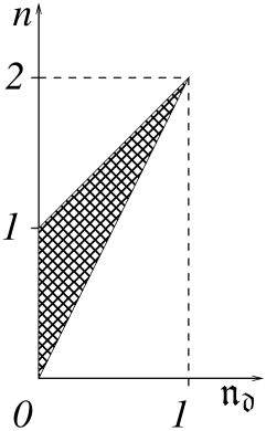
Figure 1: Ranges of integration over the $SU(4)$ group for $n$ and $\mathfrak{n_{d}}$, Eqs. (35–39).

It is instructive to calculate the number of states on-site available for a fixed value of $n=n_{0}$:

$$\!\!\!\!\!\!\!\!\!\!\!\!{\cal N}(n_{0})=\int_{SU(4)}\!\!\!\!\!\!\!\delta(n-n_{0})d\Omega=\left\{\begin{array}[]{l}6n_{0}^{2}\,\,{\rm for}\,\,0\leq n_{0}\leq 1\,,\\ {}\\ 6(2-n_{0})^{2}\,\,{\rm for}\,\,1<n_{0}\leq 2\end{array}\right.\!\!\!\!\!\!\!\!\!\!\!$$ (40)

with $\int_{0}^{2}{\cal N}(n_{0})dn_{0}=4$, the net number of available states.

The on-site electron states in the presence of itinerant electrons are not pure in the quantum-mechanical sense, and should be described with a density matrix. If the state of the entire system corresponds to a fixed integer number of electrons (which is a possible choice, due to overall particle conservation by the Hamiltonian), this on-site density matrix will be diagonal in the number of particles on-site. In other words, there will be no off-diagonal elements involving either $|0\rangle$ or $c^{\dagger}d^{\dagger}|0\rangle$, unlike in a factorizable density matrix built out of the pure states (4). In order to restrict the trace in Eq. (30) to this subset, one should replace the generic operator ${\cal O}$ with $\sum_{n=0}^{2}{\cal P}_{n}{\cal O}{\cal P}_{n}$, where ${\cal P}_{n}$ is a projection onto a subspace with a given value of $n$ (thus ${\cal P}_{1}$ projects onto the subspace of linear combinations of $c^{\dagger}|0\rangle$ and $d^{\dagger}|0\rangle$). Obviously, operators corresponding to the physical observables on-site already have this structure. Either way, the integrand in Eq. (30) will be independent of the phases $\gamma_{c}$ and $\gamma_{cd}$ in Eq. (4), and the corresponding integration [along with the pre-factor $1/(2\pi)^{2}$] can be dropped. Thus, we finally arrive at

$$d\Omega=\frac{6}{\pi}(n-2\mathfrak{n_{d}})\sin\theta\,dnd\mathfrak{n_{d}}d\theta d\phi\,,$$ (41)

where the integration region for the four variables is still given by Eqs. (34–39).

5 Prolegomena to the mean field theory

The formalism developed in the previous sections provides necessary information about the structure of the phase space of the on-site variables $\Delta_{i}$ and $n_{d,i}$. This enables constructing a single-site mean field description for the extended FKM and related models. While postponing a truly self-consistent calculation to a future publication, we will now briefly discuss the appreciated results at a rather qualitative level. We will make the following simplifying assumptions:

(i) The system can be described in terms of a single-site energy $E$, which depends on the fluctuating values of local parameters $n$,$\mathfrak{n_{d}}$, $\theta$ and $\phi$. Here, we again omit the subscript corresponding to the chosen site, which should be viewed as embedded into a virtual crystal characterised by the average values of these parameters.

(ii) Fluctuations of both $n$ and $\mathfrak{n_{d}}$ are negligible, and their respective average values are temperature-independent. This leaves two parameters $\theta$ and $\phi$, and the integration measure is that of the SU(2) subgroup:

$$d\Omega^{\prime}=(n-2\mathfrak{n_{d}})\sin\theta d\theta d\phi\,,$$ (42)

where we omitted the unknown (and unimportant) numerical pre-factor.

(iii) On-site parameters $|\Delta|$ and $\phi$ which enter the single-site energy $E$ can be treated as classical variables. We expect this to be qualitatively correct when thermal fluctuations are sufficiently strong. At very low temperatures, on the other hand, any single-site mean-field approach would be inadequate.

(iv) The minimum of energy $E$ is attained at $|\Delta|=\Delta_{0}(T)$ and (in the ordered phase at $T<T_{c}$) at $\phi=0$. We assume that $\Delta_{0}$ equals zero above the crossover temperature $T_{\Delta}$ (where $T_{\Delta}\gg T_{c}$, see Sec. 1) and below $T_{\Delta}$ shows typical behaviour of a solution to a BCS-like gap equation:

$$\Delta_{0}(T)=\Delta_{0}(0)\sqrt{(T_{\Delta}-T)/T_{\Delta}}\,,\,\,\,T<T_{\Delta}\,.$$ (43)

Quantitatively this assumption overestimates the steepness of the crossover, as it can be argued that $\Delta_{0}(T)$ never vanishes. We write in a Ginzburg–Landau fashion,

$$E(|\Delta|,\phi)=2A\frac{T-T_{\Delta}}{T_{\Delta}}[\Delta_{0}(0)]^{2}|\Delta|^{2}+A|\Delta|^{4}-$$

$$-B(T)\cos{\phi}+\frac{1}{2}B(T)\langle\!\langle\cos{\phi}\rangle\!\rangle\,,$$ (44)

omitting terms which do not depend on $\Delta$ and $\phi$. The coefficient $A$ does not depend on temperature, whereas the molecular field $B(T)$ vanishes at $T>T_{c}$, resulting in a second-order phase transition (loss of the long-range order of the phases $\phi_{i}$) at $T_{c}$:

$$B(T)=B(0)\sqrt{(T_{c}-T)/T_{c}}\,,\,\,\,T<T_{c}\,\,.$$ (45)

Physically, $B(T)$ originates from the last term in Eq. (1). The last term in Eq. (44) offsets the usual mean-field energy double-counting, with

$$\!\!\!\!\!\!\!\!\!\!\!\!\langle\!\langle\cos{\phi}\rangle\!\rangle\equiv\frac{1}{Z}\int\cos{\phi}{\rm e}^{-E(|\Delta|,\phi)/T}d\Omega^{\prime}=\frac{I_{1}[B(T)/T]}{I_{0}[B(T)/T]}$$ (46)

at $T<T_{c}$. Here, $I_{n}$ are the imaginary argument Bessel functions, and $Z$ is the partition function,

$$Z\equiv\int{\rm e}^{-E(|\Delta|,\phi)/T}d\Omega^{\prime}\,.$$ (47)

The discontinuity of specific heat $C$ at $T_{c}$ is obtained as

$$C(T_{c}-0)-C(T_{c}+0)=\frac{1}{32}\left[B(0)/T_{c}\right]^{4}\,.$$ (48)

Formally, there are two distinct values of the angle $\theta$, corresponding to $|\Delta|=\Delta_{0}(T)$ [see Eq.(17)] . At the level of our discussion here, this appears to be due to simplifications we made in writing Eq. (44). We note, however, that this corresponds to the fact that the on-site density matrix can be parametrised by two vector (“pure-state”) components, with the two respective values of $\theta$ adding up to $\pi$ (i.e., same value of $\sin\theta$). Since both components show similar behaviour with temperature, we will follow only one of these. Assuming that the temperature is not too high, we may restrict integration over $\theta$ in Eq. (47) to $0<\theta<\pi/2$, thereby choosing the $\theta<\pi/2$ component. In the phase-disordered region between $T_{c}$ and $T_{\Delta}$, the energy $E(|\Delta|,\phi)$ can be expanded about its minimum, $|\Delta|=\Delta_{0}(T)$, yielding

$$\!\!\!\!\!\!\!\!\!\!\!\!\!Z\approx 4\left\{\frac{\pi^{3}T}{A[(n-2\mathfrak{n_{d}})^{2}-(2\Delta_{0}(T))^{2}]}\right\}^{1/2}{\rm e}^{A(\Delta_{0}(T))^{4}/T}\,,$$ (49)

provided that $T_{\Delta}-T$ is not too small, $(T_{\Delta}-T)^{2}\gg TT_{\Delta}^{2}/4A$. We find

$$\!\!\!\!\!\!\!\!\!\!\!\!\!C\!\approx \!\!\!\!\!\!\!\!\!\!\!\!\frac{1}{2}+2A[\Delta_{0}(0)]^{4}\frac{T}{T_{\Delta}^{2}}-\frac{T}{T_{\Delta}}\frac{4[\Delta_{0}(0)]^{2}}{(n-2\mathfrak{n_{d}})^{2}-4[\Delta_{0}(T)]^{2}}+$$ (50)

$$+\frac{T^{2}}{T_{\Delta}^{2}}\frac{8[\Delta_{0}(0)]^{4}}{\{(n-2\mathfrak{n_{d}})^{2}-4[\Delta_{0}(T)]^{2}\}^{2}}\,.$$

The value of $C$ increases superlinearly with temperature, and the coefficient in the $T^{2}$ term decreases smoothly as the temperature increases towards $T_{\Delta}$.

We wish to emphasise the role of the phase degree of freedom even in the disordered state above $T_{c}$. Indeed, considering $\phi$ as a fictitious variable would lead to a substitution of the integration measure $d\Omega^{\prime}$, Eq. (42), with merely $d\theta$ [replacing the integration over SU(2) subgroup with the U(1) one]. Clearly, the corresponding partition function $\tilde{Z}$ in this temperature range is given by $Z$ of Eq. (49) divided by the value of $2\pi(n-2\mathfrak{n_{d}})\sin\theta$ at the energy minimum, i.e., by $4\pi\Delta_{0}(T)$. The result for the specific heat would be

$$\tilde{C}\approx C+\frac{T}{2}\frac{2T_{\Delta}-T}{(T_{\Delta}-T)^{2}}.$$ (51)

This difference is due to the larger relative phase space volume at small $\Delta$ [which otherwise is suppressed by the weight $2|\Delta|$ entering the SU(2) integration measure, Eq. (42)]. This becomes important as the temperatures increase toward $T_{\Delta}$ and the energy $E(|\Delta|)$ , Eq. (44), softens at $\Delta=0$. Thus taking phase fluctuations into account results in a slower decrease of the average value of $|\Delta|$, and reduces the values of specific heat.

Typical numerical results for $C$ (solid line) and $\tilde{C}$ are shown in Fig. 2, whereas the corresponding average values of $|\Delta|$ are plotted in Fig. 3.

Figure 2: Typical temperature dependence of specific heat $C$ (solid line). The dotted line (plotted for $T>T_{c}$) represents $\tilde{C}$, which does not include the contribution of phase fluctuations to the partition function. Parameter values are $n-2\mathfrak{n_{d}}=0.5$, $\Delta_{0}(0)=0.125$, $B(0)=0.02$, $T_{c}/T_{\Delta}=0.01$, and $A/T_{\Delta}=10^{4}$.

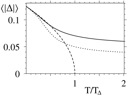
Figure 3: Thermal average of $|\Delta|$ (solid line) for the values of parameters used in Fig. 2. Dotted line shows the result obtained by neglecting phase fluctuations, whereas the dashed line corresponds to $\Delta_{0}(T)$, Eq. (43).

As mentioned above, we cannot expect to obtain a faithful description of the $T\rightarrow 0$ case, which explains the finite value of $C$ found in this limit. Following a negative jump at $T=T_{c}$, $C$ begins to increase as dictated by the second term in Eq. (50). This increase [which at higher $T$ is suppressed by terms omitted in Eq. (50)] becomes less pronounced and eventually disappears if the coefficient $A$ in Eq. (44) is decreased. As noted above, omitting phase fluctuations yields to a much stronger increase in $\tilde{C}$, with the ratio $\tilde{C}/C$ approaching 2 at the peak value (note the log scale in Fig. 2).

Above the crossover temperature $T_{\Delta}$, taking phase fluctuations into account reduces the available phase space volume near $|\Delta|=0$. This leads to stronger fluctuations of $|\Delta|$ (and accordingly yields a larger average value of $|\Delta|$) and to an increased specific heat. In fact, if the parameter values allow for the regime where

$$(n-2\mathfrak{n_{d}})^{2}\gg[\Delta_{0}(0)]^{2}\frac{T-T_{\Delta}}{T_{\Delta}}\gg\sqrt{\frac{T}{A}}\,,$$ (52)

we find

$$C\approx\frac{T_{\Delta}^{2}}{(T-T_{\Delta})^{2}}\approx 2\tilde{C}\,.$$ (53)

These results, while tentative, highlight the importance of correctly taking into account the available phase space volume in a disordered excitonic insulator above $T_{c}$. While this preliminary discussion was limited to the extended Falicov–Kimball model, we expect similar physics to play a role in related systems, including Kondo lattices.

6 Acknowledgements

The author takes pleasure in thanking A. G. Abanov, R. Berkovits, A. Frydman, A. V. Kazarnovski-Krol, and M. Khodas for discussions. This work was supported by the Israeli Absorption Ministry.

References

- [1] W. Kohn, in: Many-Body Physics, edited by C. DeWitt and R. Balian (Gordon and Breach, New York, 1967).
- [2] A. N. Kocharyan and D. I. Khomskii, Zh. Eksp. Teor. Fiz. 71, 767 (1976) [Sov. Phys. JETP 44, 404 (1976)].
- [3] H. J. Leder, Solid State Comm. 27, 579 (1978).
- [4] N. F. Mott, Phil. Mag. 30, 403 (1974).
- [5] P.Nozières and S. Schmitt-Rink, J. Low Temp. Phys. 59, 195 (1985).
- [6] J. K. Freericks and V. Zlatić, Rev. Mod. Phys. 75, 1333 (2003), and references therein.
- [7] G. Czycholl, Phys. Rev. B59, 2642 (1999).
- [8] C. D. Batista, Phys. Rev. Lett. 89, 166403 (2002).
- [9] P. Farkašovský, Phys. Rev. B77, 155130 (2008).
- [10] D. I. Golosov, Phys. Rev. B86, 155134 (2012).
- [11] V. Apinyan and T. K. Kopeć, J. Low Temp. Phys. 176, 27 (2014).
- [12] P. Coleman, Introduction to Many-Body Physics (Cambridge University Press, Cambridge, 2015), and references therein.
- [13] M. Randeria, in: Models and Phenomenology for Conventional and High-Temperature Superconductivity (Proceedings of the International School of Physics “Enrico Fermi”, Course 136), edited by G. Iadonisi, J. R. Schriffer, and M. L. Chiofalo (IOS Press, Amsterdam, 1998), and references therein.
- [14] Q. Chen, J. Stajic, S. Tan, and K. Levin, Phys. Rep. 412, 1 (2005), and references therein.
- [15] V.-N. Phan, H. Fehshke, and K. W. Becker, Europhys. Lett. 95, 17006 (2011), and references therein.
- [16] C. Schneider and G. Czycholl, Eur. Phys. J. B64, 43 (2008).
- [17] T. Tilma, M. Byrd, and E. C. G. Sudarshan, J. Phys. A: Math. Gen. 35, 10445 (2002).
- [18] A. Auerbach, Interacting Electrons and Quantum Magnetism (Springer, New York, 1994), and references therein.