Eigenvalue approximation of sums of Hermitian matrices from eigenvector localization/delocalization

Abstract

We propose a technique for calculating and understanding the eigenvalue distribution of sums of random matrices from the known distribution of the summands. The exact problem is formidably hard. One extreme approximation to the true density amounts to classical probability, in which the matrices are assumed to commute; the other extreme is related to free probability, in which the eigenvectors are assumed to be in generic positions and sufficiently large. In practice, free probability theory can give a good approximation of the density.

We develop a technique based on eigenvector localization/delocalization that works very well for important problems of interest where free probability is not sufficient, but certain uniformity properties apply. The localization/delocalization property appears in a convex combination parameter that notably, is independent of any eigenvalue properties and yields accurate eigenvalue density approximations.

We demonstrate this technique on a number of examples as well as discuss a more general technique when the uniformity properties fail to apply.

I Summary of the main results

This paper proposes an answer to an applied mathematics problem with a rich pure history: what are the eigenvalues of the sum of two symmetric matrices? Knutson and Tao remind us knutson2001honeycombs that in 1912 Hermann Weyl asked for all the possible eigenvalues that can result given the eigenvalues of the summands weyl1912asymptotische . We ask a less precise question that we suspect may also be more useful. What might the spectrum (as a distribution) look like?

Let us start by the eigenvalue decompositions of two $m\times m$ self-adjoint matrices $M_{1}=Q_{1}^{-1}\Lambda_{1}Q_{1}$ and $M_{2}=Q_{2}^{-1}\Lambda_{2}Q_{2}$ where $\Lambda_{1}$ and $\Lambda_{2}$ are diagonal matrices of eigenvalues of $M_{1}$ and $M_{2}$, and $Q_{1}$ and $Q_{2}$ are $\beta-$orthogonal matrices with $\beta=1,2,4$ denoting real orthogonal, unitary and symplectic respectively. The goal then becomes to compute the eigenvalue distribution of $M\equiv M_{1}+M_{2}$ from the knowledge of the distributions of $\Lambda_{1}$ and $\Lambda_{2}$.

Let us change basis and write $M_{1}+M_{2}$ as

$$M\equiv\Lambda_{1}+Q_{s}^{-1}\Lambda_{2}Q_{s},$$ (1)

where $Q_{s}\equiv Q_{2}Q_{1}^{-1}$.

Let us define the classical and finite free versions of this problem, respectively, by

$$M_{c} = \Lambda_{1}+\Pi^{-1}\Lambda_{2}\Pi$$ (2)

$$M_{f} = \Lambda_{1}+Q^{-1}\Lambda_{2}Q$$ (3)

where $\Pi$ denotes a uniform random permutation matrix and $Q$ is a $\beta-$Haar orthogonal matrix. Note that we only replaced the exact $Q_{s}$ in Eq. (1) with the appropriate approximations. That is $\Lambda_{1}$ and $\Lambda_{2}$ are kept the same in $M_{c}$, and $M_{f}$.

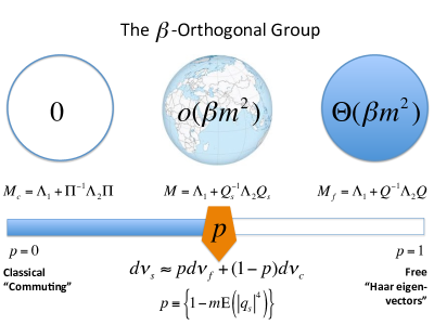
Figure 1: Depiction of the proposition. Inside the spheres we show the parameter count for the corresponding $\beta-$orthogonal matrix

Remark 1.

The eigenvalue distribution of $M_{c}$ and $M_{f}$ are, respectively, the classical and finite “free” convolution of the distributions corresponding to $\Lambda_{1}$ and $\Lambda_{2}$.

Let $d\nu_{1}$ and $d\nu_{2}$ be the eigenvalue densities of $M_{1}$ and $M_{2}$ respectively. By assumption the distribution of $M$, denoted by $d\nu_{M}$, is hard to compute. The notation we use for the classical and finite free convolutions of $d\nu_{1}$ and $d\nu_{2}$ respectively is

$$d\nu^{c} = d\nu_{1}\boxplus_{c}\mbox{ }d\nu_{2}\qquad\mbox{classical}$$ (4)

$$d\nu^{f} = d\nu_{1}\boxplus_{f}\mbox{ }d\nu_{2}\qquad\mbox{Free}.$$ (5)

Classical approximation assumes that $M_{1}$ and $M_{2}$ commute (Eq. (2)), whereas, the free approximation (Eq. (3)) is the extreme opposite in the sense that in $M_{f}$ the relative eigenvectors are in completely generic positions. Moreover, the number of random parameters in $\Pi$ and $Q$ are the minimum and maximum possible respectively (Fig. (1)). These observations motivate the proposal that the actual problem is in-between.

There is a line, the convex combination, that connects these two extremes that is both mathematically natural and in practice very powerful for obtaining the density of the sum. We denote it by

$$d\nu^{(p)}\equiv d\nu_{1}\boxplus_{p}d\nu_{2}=p\mbox{ }d\nu^{f}+(1-p)\mbox{ }d\nu^{c}\quad$$ (6)

for $0\leq p\leq 1$. Note that $d\nu^{(0)}\equiv d\nu^{c}$ and $d\nu^{(1)}=d\nu^{f}$.

Many applied problems involve summing random objects whose measures are $d\nu_{1}$ and $d\nu_{2}$. We hypothesize that very often the measure of the sum is well approximated by either $d\nu^{(1)}$ or $d\nu^{(p)}$ for some $0\leq p\leq 1$, where we describe how to obtain the appropriate parameter $p$.

We define the $k^{th}$ empirical moment of $M$ by

$$m_{k}=\varphi[M^{k}]=\frac{1}{m}\mathbb{E}\text{Tr}[M^{k}].$$ (7)

We find that $\mathbb{E}\text{Tr}(M^{k})=\mathbb{E}\text{Tr}(M_{c}^{k})=\mathbb{E}\text{Tr}(M_{f}^{k})$ for $k=1,2,3$, i.e., the fourth moment is where the three problems distinguish themselves. Therefore, we define $p$ by matching fourth moments

$$m_{4}=pm_{4}^{f}+(1-p)m_{4}^{c}\text{ },$$ (8)

where $m_{4}\equiv\varphi(M^{4})$, $m_{4}^{c}\equiv\varphi(M_{c}^{4})$, and $m_{4}^{f}\equiv(M_{f}^{4})$ need to be calculated exactly to solve for $p$, which using the above equation is simply

$$p=\frac{m_{4}^{c}-m_{4}}{m_{4}^{c}-m_{4}^{f}}=\frac{\varphi(M_{c}^{4})-\varphi(M^{4})}{\varphi(M_{c}^{4})-\varphi(M_{f}^{4})}.$$ (9)

So far in this section, the problem setup has been completely general. An interesting and a surprisingly simple and general formula for $p$ can be derived if we make an assumption (Assumption (1)). In practice the domain of applicability of this technique (Eqs. (6) and (9)) extends beyond.

Definition 1.

We say the eigenvector matrix $U$ is permutation invariant, when given two permutation matrices $\Pi_{1}$ and $\Pi_{2}$, the joint distribution of the entries of $U$ and the joint distribution of the entries of $\Pi_{1}U\Pi_{2}$ are the same.

Assumption 1.

In Eq. (1), $\Lambda_{1}$ and $\Lambda_{2}$ are independent random diagonal matrices. $Q_{s}$ is random and permutation invariant (but not necessarily Haar).

Proposition.

Under this assumption, the eigenvalues density of $M$ is approximated by $d\nu_{M}\approx d\nu^{(p)}$, where $d\nu^{(p)}\equiv pd\nu^{f}+(1-p)d\nu^{c}$. The parameter $0\leq p\leq 1$ is defined by

$$p=\frac{m_{4}^{c}-m_{4}}{m_{4}^{c}-m_{4}^{f}}=\frac{\left\{1-m\mathbb{E}\left(|q_{s}|^{4}\right)\right\}}{\left\{1-m\mathbb{E}\left(|q|^{4}\right)\right\}}\text{ }\overset{m\rightarrow\infty}{=}\text{ }1-m\mathbb{E}(|q_{s}|^{4}),$$ (10)

where $q_{s}$ denotes any entry of $Q_{s}$, and $q$ denotes any entry of the $\beta-$Haar $Q$.

We were surprised to find that $p$ is independent of the eigenvalue distributions and in that sense is universally given by Eq. (10) as long as the eigenvectors are permutational invariant.

Remark 2.

In the finite case, in Eq. (10) we have a ratio of $1-m\mathbb{E}\left(|q_{s}|^{4}\right)$ and $1-m\mathbb{E}\left(|q|^{4}\right)$. These are measures of the localization of the eigenvectors of $Q_{s}$ and $Q$ respectively, and in physics literature are called inverse participation ratios. Let us illustrate this by taking a general eigenvector matrix $U$ and denote any column of it by $u$. Denote its entries by $u_{i}$. Since $\mathbb{E}(|u_{i}|{}^{2})=(1/m)\sum_{i}|u_{i}|^{2}=1$ and, because of centrality $\mathbb{E}(u_{i}^{3})=0$ , a good measure for distribution of entries of $u$ is

$$1-m\mathbb{E}(|u_{i}|^{4})=1-\sum_{i=1}^{m}|u_{i}|^{4}=\left\{\begin{array}[]{cccc}0&&u=(0,\dots,0,1,0,\dots,0)^{T}&\text{most localized},\\ 1-1/m&&u=\frac{1}{\sqrt{m}}(1,1,\dots,1)&\text{most delocalized}.\end{array}\right.$$

As $m\rightarrow\infty$ the inverse participation ratio goes to $1$ for the most delocalized eigenvectors. It is fascinating that in quantifying localization and teasing apart the difference among empirical measures, the fourth moment is what matters most.

Illustration

We provide two illustrations of this theory that are relevant in quantum many-body systems (see Fig. (2)) and defer the details and further examples to Section VI. The Figure on the left shows the density of states (DOS) of a quantum spin chain with generic local interactions in which $p=0.43$. The example on the right is the DOS of the Anderson model in which $p=1$ (i.e., the free approximation suffices).

      

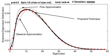
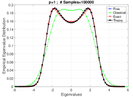
Figure 2: Left: Density of states (DOS) of a quantum spin chain with generic local interactions movassagh2011density . Here $p=0.43$, the solid grey curve is the DOS of the free approximation (i.e, $p=1$) and dashed grey curve is the DOS of classical version ($p=0$). The red dots are the exact DOS and the black solid line is the approximation obtained from our technique. Right: DOS of the Anderson model with $p=1$. Sum of a diagonal standard random gaussian matrix, $M_{1}$, and the hopping matrix, $M_{2}=Q^{T}(2\mathbb{I}+L)Q$, where $L$ is the Laplacian matrix. Please see Section VI for the details.

II Introduction

Given the eigenvalues of two $m\times m$ Hermitian matrices, how does one determine all the possible set of the eigenvalues of the sum? As stated at the very beginning of this paper, H. Weyl’s question lead to many mathematical developments and A. Horn’s seminal work that conjectured a (over-complete) set of recursive inequalities for the eigenvalues of sums of Hermitian matrices horn1962eigenvalues . This conjecture was proved by Klyachko klyachko1998stable and later made clearer with the use of Schubert calculus by Knudson and Tao knutson2001honeycombs . However, the bounds obtained from these works are not very good for sparse matrices which are often encountered in practice (e.g., local Hamiltonians that physicists often consider). In any case and despite these great successes, there are not many results that with a high accuracy compute the eigenvalues of the sum from the knowledge of the summands.

Our goal is pragmatic: we seek a method that enables us to draw (on a computer) an accurate picture of the density of the eigenvalues of the sum from those of the summands.

Given the probability measures $d\nu_{1}$ and $d\nu_{2}$ of two random variables, one can ask: what is the measure of the sum of the random variables? In classical probability theory in which the random variables commute, the measure of the sum is the convolution of the measures. In the other extreme, where the random variables do not commute and are generic (e.g., random matrices), the measure in the infinite limit is the free convolution nica2006lectures ; voiculescu1992free .

Let us define the $\varphi$ notation following nica2006lectures . Let ${\cal A}$ be unital algebras over $\mathbb{C}$ . The elements of ${\cal A}$ are in general non-commuting.

Definition 2.

Let $\varphi$ be a unital linear functional $\varphi:\text{ }{\cal A}\rightarrow\mathbb{C}$, with the properties that $\varphi$ is a trace and $\varphi[1_{{\cal A}}]=1$. $\varphi$ is a trace in the sense that

$$\varphi[ab]=\varphi[ba],\quad\forall a,b\in{\cal A},$$

Let $\varphi_{c}$ be the “commutative” version of $\varphi$, that has the additional property that the order of the product of its arguments do not matter, i.e., $\varphi_{c}[abc]=\varphi_{c}[bac]=\cdots$.

Notation 1.

When the variables (elements of ${\cal A})$ are $m\times m$ matrices, then

$$\begin{array}[]{ccc}\varphi[\centerdot]\equiv\frac{1}{m}\text{Tr}[\centerdot]&&\text{non-random matrices}\\ \\ \varphi[\centerdot]\equiv\frac{1}{m}\mathbb{E}\text{Tr}[\centerdot]&&\text{random matrices .}\\ \\ \varphi[\centerdot]=\int\centerdot\text{ }d\mu&&\text{operators}\end{array}$$

Given a random matrix $M$, the expected empirical measure of its eigenvalues is

$$d\nu_{M}=\varphi[M]=\frac{1}{m}\mathbb{E}\left\{\sum_{i=1}^{m}\delta\left(\lambda-\lambda_{i}(M)\right)\right\}.$$

II.1 Introduction to Free Probability Theory

Free probability theory (FPT) is suited for non-commuting random variables. The more conventional probability theory (CPT) deals with commuting random variables.

Supposed $M_{1},M_{2},\cdots,M_{N}$ are $m\times m$ random matrices with known eigenvalue distributions, what is the eigenvalue distribution of

$$M=M_{1}+M_{2}+\cdots+M_{N}\quad?$$ (11)

FPT answers this question if $M_{k}$’s are free. We define free independence following Nica and Speicher nica2006lectures .

Definition 3.

([Nica Speicher] Free Independence) Let $({\cal A},\varphi)$ be a non-commutative probability space and let $I$ be a fixed index set. The subalgebras $({\cal A}_{i})_{i\in I}$ are called free independent with respect to the functional $\varphi$, if

$$\varphi(a_{1}\dots a_{k})=0$$

whenever we have the following:

• $k$ is a positive integer;

• $a_{j}\in{\cal A}_{i(j)}$ , $(i(j)\in I)$ for all $j=1,\dots,k$;

• $\varphi(a_{j})=0$ for all $j=1,\dots,k$;

• and neighboring elements are from different subalgebras, i.e., $i(1)\neq i(2)$, $i(2)\neq i(3)$, $\dots$, $i(k-1)\neq i(k)$.

Recall that in CPT the distribution of sum of random variables is not additive but the cumulants or log-characteristics are. The analogous additive quantities in FPT are free cumulants and $r-$transforms nica2006lectures .

How can we make utilize FPT to analytically obtain the eigenvalue distribution of Eq. (11)? As long as $M_{k}$’s are free from one another, theoretically, the free convolution will provide the distribution of the sum. However, its numerical computation may be difficult.

For the sake of concreteness, suppose we have two matrices $M_{1}$ and $M_{2}$ , which may not be free, and we are interested in the spectrum of the sum

$$M=M_{1}+M_{2};$$ (12)

the free approximation can be obtained by (possibly slightly) changing the problem. Mathematically, FPT would obtain the eigenvalue distribution of

$$M_{1}+Q^{-1}M_{2}Q$$

where, $Q$ is an $m\times m$ Haar distributed $\beta-$orthogonal matrix as before. This amounts to spinning the eigenvectors to point randomly and uniformly on a sphere in orthogonal group $\mathcal{O}(m)$ uniformly. Our technology can treat both finite and infinite matrices. One need not use the standard fields; arbitrary number fields can be used by replacing $Q$ in Eq. (12) by the corresponding Haar matrices (see Table (1)).

Field	Real	Complex	Quaternions	“Ghosts”
$\beta$	$1$	$2$	$3$	$>3$
Haar matrices	$Q$	$U$	$S$	$\mathcal{G}$

Table 1: Notation for various fields of numbers

Remark 3.

Standard FPT proves that $M_{1}$ and $Q^{-1}M_{2}Q$ are asymptotically free. If we look at the moments of the sum, i.e., $\varphi\left[M_{1}+Q^{-1}M_{2}Q\right]^{k}=\frac{1}{m}\mathbb{E}\text{Tr}\left[M_{1}+Q^{-1}M_{2}Q\right]^{k}$ then $O(1)$ terms would match the answer that FPT would provide and there will be additional terms (finite corrections) that will be at most $O(1/m)$.

Since its eigenvectors are Haar, one naturally thinks of the free approximation as the most delocalized. For finite Haar distributed $\beta-$orthogonal matrices (compare with Eq. (10)),

$$1-m\mathbb{E}(|q|^{4})=\frac{(m-1)\beta}{m\beta+2}$$ (13)

which in the limit of $m\rightarrow\infty$ is independent of $\beta$ and equal to one. More generally, for $\beta-$Haar orthogonal matrix of size $m\times m$ we have

Moments of $\beta-$Haar Orthogonal matrix
Expected values	Count
$\mathbb{E}(|q_{i,j}|^{2})=1/m$	$m^{2}$
$\mathbb{E}(|q_{i,j}|^{4})=\frac{\beta+2}{m(m\beta+2)}$	$m^{2}$
$\mathbb{E}(|q_{i,j}|^{2}|q_{i,k}|^{2})=\frac{\beta}{m(m\beta+2)}$, $j\neq k$	$2m^{2}(m-1)$
$\mathbb{E}(\bar{q}_{ji}q_{jk}\bar{q}_{pk}q_{pi})=\frac{-\beta}{m(m\beta+2)(m-1)}$, $i\neq k\text{ and }j\neq p$	$m^{2}(m-1)^{2}$

Comment: These formulas can be derived from Weingarten formulas or direct calculations for $\beta=1,2,4$. We have checked the quantities in the table above against numerical experiments for $\beta=1,2$. General $\beta\notin\{1,2,4\}$ is a subject of current speculation.

III More than two matrices

In our work we satisfy ourselves with sums of two hermitian matrices. However, in the next two subsections we provide results that extend the moment computation for the classical and free modifications of the problem.

III.1 Classical irreducible moment expansion

Definition 4.

(Classically Equivalent) In the expansion of $\varphi_{c}\left[\left(M_{1}+M_{2}+\dots+M_{k}\right)^{n}\right]$, there are $k^{n}$ monomials that can be put into distinct equivalent classes under $\varphi_{c}$. Each equivalence class is defined by the distinct set of positive integers $j_{i}\in[n]$ for $1\leq i\leq k$, where any fixed set $j_{1},\dots,j_{k}$ corresponds to the number of times $M_{1},\dots,M_{k}$ appear in the expansion respectively.

Because of the commutativity, the binomial theorem can be evoked, and by the cyclic property of $\varphi_{c}$

$$\varphi_{c}\left[\left(M_{1}+M_{2}\right)^{n}\right]=\sum_{j=0}^{n}\left(\begin{array}[]{c}n\\ j\end{array}\right)\varphi_{c}\left[M_{1}^{j}M_{2}^{n-j}\right],$$ (14)

where each summand is the contribution of the $j^{\text{th}}$ equivalent class. More generally,

$$\varphi_{c}\left[\left(M_{1}+M_{2}+\cdots+M_{k}\right)^{n}\right]=\sum_{j_{1}+\cdots+j_{k}=n}\left(\begin{array}[]{ccccc}&&n\\ j_{1}&,&\cdots&,&j_{k}\end{array}\right)\varphi_{c}\left[M_{1}^{j_{1}}M_{2}^{j_{2}}\dots M_{k}^{j_{k}}\right],$$

where each summand once again is the contribution of one of the equivalent classes.

We wish to generalize these classical notions to the non-commutative setting, whereby the reduced form of the non-classical (i.e., non-commuting) moment expansion $\varphi\left[\left(A+B\right)^{n}\right]$ is found. As a first step, it would be helpful to know the number of terms of each type that are cyclically equivalent with respect to $\varphi$.

III.2 Free irreducible moment expansion

Definition 5.

(trace-equivalent) In the general non-commuting $n^{th}$ moment expansion

$$\varphi\left[(M_{1}+M_{2}+\cdots+M_{k})^{n}\right]$$ (15)

there are $n^{k}$ monomials each of which is a product of $n$ terms chosen from the alphabet $\{M_{1},M_{2},\dots,M_{k}\}$. We define each trace-equivalent class to be the subset of monomials that are equal under $\varphi$.

So how many of such equivalent classes are there? The answer to this question is equivalent to a theorem by Polya riordan2012introduction .

Definition.

An $(n,k)$-necklace is an equivalence class of words of length $n$ over an alphabet of size $k$ under rotation (i.e., cyclically equivalent). The total number of such distinct necklaces is denoted by $a(n,k)$.

Theorem.

(Polya) Let $\phi(d)$ be the Euler function of the positive integer $d$ and $d|n$ denote all the divisors of the integer $n$ then

$$a(n,k)=\frac{1}{n}\sum_{i=1}^{n}k^{\text{gcd}(n,i)}=\frac{1}{n}\sum_{d|n}\phi(d)k^{n/d}.$$

For example, in $\varphi\left[(M_{1}+M_{2})^{n}\right]$ there are $a(n,2)$ necklaces. More generally, in $\varphi\left[(M_{1}+M_{2}+\cdots+M_{k})^{n}\right]$ there are $a(n,k)$ necklaces. In Fig. (3) we illustrate the equivalent classes of $a(3,2)$ and $a(4,2)$. The former corresponds to $\varphi\left[(M_{1}+M_{2})^{3}\right]$ and the latter to $\varphi\left[(M_{1}+M_{2})^{4}\right]$.

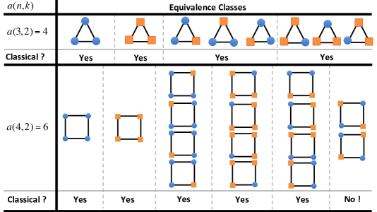
Figure 3: Illustration of Theorem. The one-to-one correspondence with moment expansion in Eq. (15) can be done by thinking of circles as $M_{1}$ and squares as $M_{2}$.

Lemma 1.

In the expansion $\varphi\left[(M_{1}+M_{2})^{n}\right]$ there are only $(n-1)^{2}+1$ terms that are classical.

Proof.

These would coincide with the terms that are cyclically equal to $\varphi_{c}\left[M_{1}^{j}M_{2}^{n-j}\right]$. Suppose $M_{1}$ appears $j$ times. If $0<j<n$ the length of the cyclic orbit is exactly $n$. However, if $j=0$ or $j=n$, then there is no orbit and each has exactly one term in the corresponding equivalence class. We have altogether $(n-2)n+2$ classical terms. ∎

IV Technical Results

We now return to the problem of approximating the eigenvalue distribution of sums of two hermitian matrices. Below we use $U$ to denote an eigenvector matrix that is permutation invariant and $\beta-$orthogonal; it can be $Q_{s}$, $\Pi$ or $Q$. That is we reserve $U$ when the results being proved do not depend on the choice of the three cases. We assume that the columns of $U$ are chosen so that each column and its negation are equiprobable. One consequence is that the mean of every element of $U$ is zero. Below repeated indices are summed over unless states otherwise. We denote the (diagonal) entries of $\Lambda_{1}$ and $\Lambda_{2}$ by

$$\lambda_{i} \rightarrow \Lambda_{1}$$

$$\mu_{i} \rightarrow \Lambda_{2}$$

Lemma 2.

The elements of $U$ are (dependent) random variables with mean zero and variance $1/m$.

Proof.

The invariance under the change of sign implies the zero mean. The variance is $\frac{1}{m^{2}}\sum|u_{ij}|^{2}=1/m$. ∎

Lemma 3.

(departure lemma) $\varphi\left[\Lambda_{1}^{k_{1}}U^{-1}\Lambda_{2}^{k_{2}}U\right]=\mathbb{E}\left(\lambda_{i}^{k_{1}}\right)\mathbb{E}\left(\mu_{j}^{k_{2}}\right)$.

Proof.

By permutation invariance and Lemma (2), $\mathbb{E}(|u_{ij}|^{2})=1/m$ . For integers $k_{1}>0$ and $k_{2}>0$, we have $\mathbb{E}\textrm{Tr}\left(\Lambda_{1}^{k_{1}}U^{-1}\Lambda_{2}^{k_{2}}U\right)=\mathbb{E}\left(\sum_{i,j}|u_{ij}|^{2}\lambda_{i}^{k_{1}}\mu_{j}^{k_{2}}\right)$. By the independence of the eigenvalues from the eigenvectors, this expected value is equal to $m^{2}\left(\frac{1}{m}\right)\mathbb{E}\left(\lambda_{i}^{k_{1}}\mu_{j}^{k_{2}}\right)$ for any $i$ or $j$. By Def. (2), we now have

$$\varphi\left[\Lambda_{1}^{k_{1}}U^{-1}\Lambda_{2}^{k_{1}}U\right]=\mathbb{E}\left(\lambda_{i}^{k_{1}}\mu_{j}^{k_{2}}\right)=\mathbb{E}\left(\lambda_{i}^{k_{1}}\right)\mathbb{E}\left(\mu_{j}^{k_{2}}\right),$$

where the last equality follows from the independence of $\Lambda_{1}$ and $\Lambda_{2}$. ∎

Lemma 4.

The first three moments of $\Lambda_{1}+U^{-1}\Lambda_{2}U$ are equal (and independent of the distribution of $U$).

Proof.

Using the trace property $\text{Tr}(AB)=\text{Tr}(BA)$, the first three moments are

$$\begin{array}[]{c}m_{1}\equiv\varphi\left[\Lambda_{1}+\Lambda_{2}\right]\qquad\text{in all three cases}\\ m_{2}\equiv\varphi\left[\left(\Lambda_{1}+U^{-1}\Lambda_{2}U\right)^{2}\right]=\varphi\left(\Lambda_{1}^{2}+2\Lambda_{1}U^{-1}\Lambda_{2}U+\Lambda_{2}^{2}\right)\\ m_{3}\equiv\varphi\left[\left(\Lambda_{1}+U^{-1}\Lambda_{2}U\right)^{3}\right]=\varphi\left(\Lambda_{1}^{3}+3\Lambda_{1}^{2}U^{-1}\Lambda_{2}U+3\Lambda_{1}U^{-1}\Lambda_{2}^{2}U+\Lambda_{2}^{3}\right),\end{array}$$

By linearity of the $\mathbb{E}\text{Tr}(\centerdot)$ and Lemma (3) $m_{1}$, $m_{2}$ and $m_{3}$ above are all equal to the corresponding classical first, second and third moments respectively. ∎

The fourth moments of the three cases will differ because of the appearance of the terms that we put in bold-faced and underlined in.

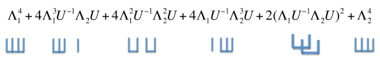
Figure 4: Fourth moment expansion and (non)-crossing partitions. We represent each $\Lambda_{1}$ with a vertical line and connect products of $\Lambda_{1}$ by a horizontal line (similarly with $U^{-1}\Lambda_{2}U$). Note that $(\Lambda_{1}U^{-1}\Lambda_{2}U)^{2}$ is the only crossing partition, and is the only term whose expected trace differs among the three cases. The crossing partitions appear first in the fourth moment expansions.

$$m_{4}\equiv\varphi\left[\left(\Lambda_{1}+U^{-1}\Lambda_{2}U\right)^{4}\right]=\varphi\left[\Lambda_{1}^{4}+4\Lambda_{1}^{3}U^{-1}\Lambda_{2}U+4\Lambda_{1}^{2}U^{-1}\Lambda_{2}^{2}U+4\Lambda_{1}U^{-1}\Lambda_{2}^{3}U+\mathbf{\underline{2\left(\mathbf{\Lambda_{1}U^{-1}\Lambda_{2}U}\right)^{2}}}+\Lambda_{2}^{4}\right].$$ (16)

In Fig. (4) we express these terms in their natural combinatorial representation in terms of (non)-crossing partitions.

Let the symmetric polynomials of degree $k$ in $m$ variables be denoted by $SP(k,m)$. Moreover let $\lor$ denote a symmetric product, which we take to mean that the product is invariant under exchange, i..e, $x\lor y=y\lor x$. Moreover, let $\kappa_{2}(\Lambda)=\frac{1}{m}\sum_{i}\lambda_{i}^{2}-\left(\frac{\sum\lambda_{i}}{m}\right)^{2}$, which is the “variance” of $(\lambda_{1},\lambda_{2},\dots,\lambda_{m})$.

Lemma 5.

Let $f(\Lambda_{1},\Lambda_{2})\in SP(k,m)\lor SP(k,m)$ such that $f(\mathbb{I},\Lambda_{2})=0$. Then if $k=2$, $f(\Lambda_{1},\Lambda_{2})=c\text{ }\kappa_{2}(\Lambda_{1})\kappa_{2}(\Lambda_{2})$, where $c$ is a constant.

Proof.

It is clear that $f$ as a polynomial in $\Lambda_{1}$ is a multiple of $\kappa_{2}(\Lambda)$ because $f$ vanishes at $\Lambda_{1}=\mathbb{I}$ and $SP(2,m)$ is only two-dimensional. Similarly $f$ is a multiple of $\kappa_{2}(\Lambda_{2})$ as a polynomial in $\Lambda_{2}$. Since $f$ vanishes at $\Lambda_{2}=\mathbb{I}$ the only polynomials in $SP(2,m)\lor SP(2,m)$ with this property are multiples of $\kappa_{2}(\Lambda_{1})\kappa_{2}(\Lambda_{2})$. ∎

The following lemma is key:

Lemma 6.

$\varphi\left[\left(\Lambda_{1}+\Pi^{-1}\Lambda_{2}\Pi\right)^{4}-\left(\Lambda_{1}+U^{-1}\Lambda_{2}U\right)^{4}\right]=\kappa_{2}(\Lambda_{1})\kappa_{2}(\Lambda_{2})\left\{1-m\mathbb{E}\left(|u_{ij}|^{4}\right)\right\}.$

Proof.

$U=\Pi$ is trivial so we think of $U$ as a place holder for $Q_{s}$ and $Q$. Because of the linearity of $\varphi$ and Lemma (3) the general form of this difference is

$$\varphi\left[\left(\Lambda_{1}+\Pi^{-1}\Lambda_{2}\Pi\right)^{4}-\left(\Lambda_{1}+U^{-1}\Lambda_{2}U\right)^{4}\right] = 2\varphi\left[\left(\Lambda_{1}\Pi^{-1}\Lambda_{2}\Pi\right)^{2}-\left(\Lambda_{1}U^{-1}\Lambda_{2}U\right)^{2}\right],$$ (17)

where the expectation is taken with respect to the random permutations $\Pi$ and eigenvectors $U$ respectively.

In Eq. (17) if $\Lambda_{1}\rightarrow\alpha\Lambda_{1}$ then the right hand side gets multiplied by $\alpha^{2}$, so it is a homogenous polynomial of second order. Since conjugating either $\Lambda_{1}$ or $\Lambda_{2}$ by any permutation matrix leaves the expected trace invariant, the expression is a symmetric polynomial in entries of $\Lambda_{1}$ and $\Lambda_{2}$. Therefore, by Lemma (5), we have

$$\varphi\left[\left(\Lambda_{1}\Pi^{-1}\Lambda_{2}\Pi\right)^{2}-\left(\Lambda_{1}U^{-1}\Lambda_{2}U\right)^{2}\right]=c(U)\text{ }\kappa_{2}(\Lambda_{1})\kappa_{2}(\Lambda_{2}).$$

To evaluate $c\left(U\right)$, it suffices to let $\Lambda_{1}$ and $\Lambda_{2}$ be projectors of rank one where $\Lambda_{1}$ would have only one nonzero entry on the $i^{\mbox{th }}$ position on its diagonal and $\Lambda_{2}$ only one nonzero entry on the $j^{\mbox{th }}$ position on its diagonal. Further take those nonzero entries to be ones, giving $m_{1,1}^{\lambda}=m_{1,1}^{\mu}=0$ and $m_{2}^{\lambda}=m_{2}^{\mu}=1/m$, and we have

$$\varphi\left[\left(\Lambda_{1}\Pi^{-1}\Lambda_{2}\Pi\right)^{2}-\left(\Lambda_{1}U^{-1}\Lambda_{2}U\right)^{2}\right]=\frac{1}{m^{2}}\text{ }c\left(U\right).$$ (18)

But the left hand side is

$$\varphi\left[\delta_{ij}-|u_{ij}|^{4}\right] = \frac{1}{m}\left\{\frac{1}{m^{2}}\sum_{ij}\delta_{ij}-\frac{1}{m^{2}}\sum_{ij}\mathbb{E}\left(|u_{ij}|^{4}\right)\right\}=\frac{1}{m}\left\{\frac{1}{m}-\mathbb{E}\left(|u_{ij}|^{4}\right)\right\},$$

where we used the homogeneity of $U$. Consequently, by equating this to $c\left(U\right)/m^{2}$, we get the desired quantity

$$c\left(U\right)=\left\{1-m\mathbb{E}\left(|u_{ij}|^{4}\right)\right\}.$$

Our final result, i.e., Eq. (17), reads

$$\varphi\left[\left(\Lambda_{1}\Pi^{-1}\Lambda_{2}\Pi\right)^{2}-\left(\Lambda_{1}U^{-1}\Lambda_{2}U\right)^{2}\right]=\kappa_{2}(\Lambda_{1})\kappa_{2}(\Lambda_{2})\left\{1-m\mathbb{E}\left(|u_{ij}|^{4}\right)\right\}.$$ (19)

where $\kappa_{2}(\Lambda_{1})=\left(m_{2}^{\lambda}-m_{1,1}^{\lambda}\right)$ and $\kappa_{2}(\Lambda_{2})=\left(m_{2}^{\mu}-m_{1,1}^{\mu}\right)$ as before. ∎

Theorem 1.

(universality of $p$) In defining $p$ by matching fourth moments via $m_{4}=pm_{4}^{f}+(1-p)m_{4}^{c}$, we find that $p$ is independent of the eigenvalues and is given by

$$p=\frac{m_{4}^{c}-m_{4}}{m_{4}^{c}-m_{4}^{f}}=\frac{\left\{1-m\mathbb{E}\left(|q_{s}|^{4}\right)\right\}}{\left\{1-m\mathbb{E}\left(|q|^{4}\right)\right\}}\text{ }\overset{m\rightarrow\infty}{=}\text{ }\left\{1-m\mathbb{E}\left(|q_{s}|^{4}\right)\right\},$$ (20)

where, as before, $q_{s}$ and $q$ denote any entry of $Q_{s}$ and $Q$ respectively (see Eqs. (1) and (3)).

Proof.

The first equality follows the definition of $p$ via fourth moment matching. The second equality follows Lemma (6) , where the dependence on eigenvalues as well as an overall factor of $2$ that appear in the numerator and the denominator cancel. The last equality follows Eq. (13) in the limit of $m\rightarrow\infty$, which corresponds to free probability theory. ∎

Corollary 1.

(Slider) $0\leq p\leq 1$.

Proof.

Since by normality of eigenvectors $\sum_{i=1}^{m}|q_{s}^{i}|^{2}=1$, we have that $0\leq\sum_{i=1}^{m}|q_{s}^{i}|^{4}\leq 1$. Now $m\mathbb{E}\left(|q_{s}|^{4}\right)=m\left(\frac{1}{m}\sum_{i=1}^{m}|q_{s}^{i}|^{4}\right)$. So we have that $0\leq 1-m\mathbb{E}\left(|q_{s}|^{4}\right)\leq 1$. ∎

Comment: $p$ can analytically be calculated if one computes $\mathbb{E}(|q_{s}|^{4})$. This for example has been done for quantum spin chains with generic interactions movassagh2011density ; movassagh_IE2010 .

Remark 4.

Often in applications, one of the summands is a perturbation of the other. Namely, $M=M_{1}+\epsilon M_{2}$, where $\left\|M_{1}\right\|=\left\|M_{2}\right\|$ and $\epsilon\ll 1$. From the analysis above it should be clear that $p$ is independent of $\epsilon$.

V Computation of the Density

The eigenvalue distribution of the classical extreme is simple; one simply takes the convolution of the density of the summands. Less known and more difficult is the computation of the density of the free sum. Mathematically this is done by taking the free convolution via the $R-$transform (See nica2006lectures for a detailed discussion). However, the actual computation of the free convolution is subtle. Olver and Rao made a numerical package that works well in computing the free convolution under the assumption that the eigenvalue distribution of the summands has a connected support (it does not work as well when the support has disjoint intervals) olver2012numerical . Below we provide a complementary method for calculating the free convolution when the eigenvalues are discrete.

V.1 Density of the free sum

Suppose we seek the density of $M$ in Eq. (11) under the assumption that $M_{1},M_{2},\dots,M_{N}$ are free. This, as stated above, requires the matrices to be infinite in size. In practice, however, finite (e.g., $30\times 30$) random matrices act free.

One could fix a given matrix $M_{0}$ and take an $N-$fold free sum of it and ask: What is the density of $M$ when

$$M=Q_{1}^{\dagger}M_{0}Q_{1}+Q_{2}^{\dagger}M_{0}Q_{2}+\dots+Q_{N}^{\dagger}M_{0}Q_{N},$$ (21)

and each $Q_{i}$ is a $\beta-$Haar orthogonal matrix?

We now define a few important ingredients and outline how the density of a free sum is computed in theory. The Cauchy transform of any function, $f(x)$, is given by

$$G(z)=\frac{1}{2\pi i}\int_{\mathbb{R}}dx\text{ }\frac{f(x)}{z-x}\text{ },$$ (22)

where for our purposes we use the density $f_{k}(x)$ which denotes the distribution of the eigenvalues of $M_{k}$ in Eq. (11) (each summand is assumed to be free).

In conventional probability theory, the log-characteristics and cumulants are additive. In free probability theory, the so called $R-$transform is additive.

Using the Cauchy transform $G_{k}(z)$, the $R-$transform is defined by

$$R_{k}\left(G_{k}(z)\right)=z-\frac{1}{G_{k}(z)},$$ (23)

where in order to obtain $z$, the Cauchy transform Eq. (22) needs to be inverted. It is good practice to let $w_{k}\equiv G_{k}(z)$, by which Eq. (23) reads,

$$R_{k}(w_{k})=G_{k}^{-1}(w_{k})-\frac{1}{w_{k}};$$ (24)

in solving for $z$ in $w_{k}=G_{k}(z)$, among multiple roots one chooses the one that is consistent with $\lim_{z\rightarrow\infty}w\sim 1/z$.

Given that we find a way of inverting Eq. (22), we have in our hands the $R-$transform of each summand.

Comment: The inversion may be tedious. See the next section for a routine for doing so efficiently.

Let us denote the density of the sum by $f(x)$ and its $R-$transform by $R(w)$. As stated above, it is a fact of FPT that the $R-$transforms of the sum are additive nica2006lectures . We have

$$R(w)=\sum_{k=1}^{N}R_{k}(w)\overset{\textrm{i.d.}}{=}NR_{0}(w)$$ (25)

where the last equality only holds if each $M_{k}$ has identically distributed eigenvalues, whose $R-$transform is denoted by $R_{0}(w)$. The last equality also applies in the case of Eq. (21) where each $M_{i}=M_{0}$.

Now we have at our disposal the $R-$transform of the sum and from it we want to infer the density $f(x)$. The inverse Cauchy transform of $R(w)$ is

$$G^{-1}(w)=R(w)+\frac{1}{w}.$$

The distribution satisfies

$$w\equiv G(z)=\int_{\mathbb{R}}\frac{f(x)}{G^{-1}(w)-x}\text{ }dx.$$

Since $G^{-1}(w)$ introduces a branch cut on the real line, we perform analytical continuation into the complex plane. Let $g^{+}(z)$ be located right above the branch cut. The distribution is calculated using Plemelj-Sokhotsky formula:

$$f(x)=\frac{1}{\pi}\lim\left[\textrm{Im}(g^{+}(z)\right].$$ (26)

This completes the procedure for finding the density of the free sum of $N$ matrices.

Remark 5.

The discrete Cauchy transform of the spectrum of $M_{k}$ is $G_{k}(z)=\frac{1}{m}\underset{i=1}{\sum^{m}}\frac{1}{z-\lambda_{i}(M_{k})}$, where $\lambda_{i}(M_{k})$ is an eigenvalue of $M_{k}$. However, inverting each of the Cauchy transforms involves finding the roots of a high order complex polynomial, which can be quite difficult. In subsection V.2, we provide a routine that finds the roots efficiently without solving the high degree polynomial.

V.2 Detailed Algorithm for discrete spectra

Suppose we have a discrete distribution

$$f(x)=\frac{1}{m}\sum_{i=1}^{m}\delta(x-\lambda_{i})$$ (27)

and we want the free probability distribution of a random variables that is distributed according to an $N$-fold sum of random variables, each of which is distributed according to $f(x)$. More explicitly, suppose $M_{0}$ is distributed according to $f(x)$ in Eq. (27) and we want the distribution of Eq. (21) under the assumption that the eigenvalues of $M_{0}$ are a finite and discrete set. We now show how to obtain this by using free probability theory as an approximation.

The Cauchy distribution of $f(x)$ becomes

$$G(z)\equiv w=\frac{1}{m}\sum_{i=1}^{m}\frac{1}{z-\lambda_{i}}.$$ (28)

By the definition of the $R-$transform we can eliminate $z$ by

$$z=R(w)+\frac{1}{w};$$

we are interested in an $N-$fold free sum which by additivity of the $R$-transform amounts to $R(w)\rightarrow R(w)/N$.

The $z$ of the sum is therefore

$$z=\frac{R(w)}{N}+\frac{1}{w};$$

if one were to solve for $R(w)$, one would obtain the $R-$transform of the sum of $N$ copies the random variables.

The above procedure can succinctly be performed by only doing the following transformation on the $z$ of a single random variable

$$z\rightarrow\frac{z}{N}+\frac{1}{w}\left(1-\frac{1}{N}\right),$$

where the right hand side is the inverse Cauchy transform of the sum denoted by $G_{N}^{-1}(w)$.

The discrete inverse Cauchy transform of a sum of $N$ copies of $m\times m$ matrix $M_{0}$ (Eq. (28)) now reads

$$F(w,z,m)\equiv-w+\frac{1}{m}\sum_{i=1}^{m}\frac{1}{\frac{z}{N}+\frac{1}{w}\left(1-\frac{1}{N}\right)-\lambda_{i}}=0$$ (29)

This is the desired formula. To get the density one applies the Plemelj-Sokhotsky formula; i.e., one solves for $w$ at a fixed z, and take the imaginary part and divide by $\pi$.

Solving for $w$ as a function of $z$ requires solving a high degree polynomial, which may analytically be impossible for polynomials of degree higher than four.

After dividing through by $w$, Eq. (29) can be rewritten as

$$\sum_{i=1}^{m}\frac{v_{i}}{w-v_{i}}=\alpha,$$ (30)

where $v_{i}=\frac{N-1}{N\lambda_{i}-z}$ and denote the poles in Eq. (29) and $\alpha=-m\left(\frac{N-1}{N}\right)<0$.

The solutions of Eq. (30) correspond to the intersection of the horizontal line located at $\alpha$ with $\sum_{i=1}^{m}v_{i}/(w-v_{i})$; the latter is plotted in Fig. (5). When all the $v_{i}$ are positive or negative, there are in general exactly $m$ solutions to Eq. (30); however, when the $v_{i}$ have mixed signs, then for certain values of $\alpha$ ($\alpha>-4$ in Fig. (5)) there are $m-2$ real roots and a complex conjugate pair.

This follows because between any pair of consecutive $v_{i}$’s that are both negative (positive), the function in Eq. (30) goes from negative (positive) to positive (negative) infinity. Thus there is at least $m-2$ real solutions to Eq. (30). Therefore there are at most a complex conjugate pair of solutions. When a complex conjugate pair of solutions exist, they correspond to the solution of Eq. (30) where $v_{i}$ changes sign (see Fig. (5)).

The non-existence of a complex conjugate pair means lack of support in the distribution of the $N-$fold sum. In Plemelj-Sokhotsky formula the imaginary part needs to be taken. Lastly note, that there are at most one pair of complex conjugate roots to Eq. (30). In other words, the roots are either real (i.e. zero probability in the density) or have at most a complex conjugate pair.

How would one find the roots? There exists a matrix such that its eigenvalues are the roots (set of $w$ that are the zeros of Eq. (30)) of the above

$$\text{diag}(v_{1},\dots,v_{m})+\frac{1}{\alpha}uv^{T}\equiv\text{diag}(v)+\frac{1}{\alpha}uv^{T},$$ (31)

which is a general rank-one update, where $u=[1,\dots,1]^{T}$ is a column vector of length $m$. This is the non-symmetric generalization of the more standard secular equations method trefethen1997numerical .

To see this, assume non-singularity, which yields $\det\left(\text{diag}(v)+\frac{uv^{T}}{\alpha}-\lambda I\right)=0$ or $\det\left(I+\left(\text{diag}(v)-\lambda I\right)^{-1}\frac{uv^{T}}{\alpha}\right)=0$; therefore (using trace properties): $1+\frac{1}{\alpha}v^{T}\left(\text{diag}(v)-wI\right)^{-1}u=0$. Writing it out we have:

$$\frac{1}{\alpha}\sum_{i=1}^{m}\frac{v_{i}}{v_{i}-w}=-1$$

Therefore, eigenvalues of $\text{diag}(v)+\frac{1}{\alpha}uv^{T}$ give the roots that we were seeking .

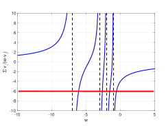
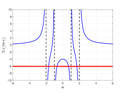
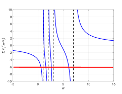
Figure 5: The red horizontal line is at $\alpha=-6$. Left: $v=[-1,-2,-3,-7]$, Middle: $v=[-2,-1,1,2]$, has mixed signs, Right: $v=[1,2,3,7]$

Remark 6.

It seems possible that one can compute the complex eigenvalues efficiently for an interval of different $z$ values by performing one initial computation, obtain the $2-$ dimensional eigenspace for a complex pair, and then update only that space with different $z$ values by an Arnoldi method.

VI Illustrations and Applications

For majority of applications involving non-commuting matrices, we believe, free probability theory suffices. However, when the latter fails, we have found that a combination of the two extreme approximations (i.e., free and classical) to work very well. In particular, under rather very mild conditions the natural parameter, $p$, for a convex combination is obtained by matching fourth moments. Below we illustrate the theory using some examples.

Let us push the analytical calculation of $p$. Using Eq. (9) we have

$$p=\frac{\mathbb{E}\text{Tr}\left[M_{c}^{4}\right]-\mathbb{E}\text{Tr}\left[M^{4}\right]}{\mathbb{E}\text{Tr}\left[M_{c}^{4}\right]-\mathbb{E}\text{Tr}\left[M_{f}^{4}\right]},$$

which by Eq. (16), and noting that in the classical approximation the summands commute, reads

$$p=\frac{\mathbb{E}\text{Tr}\left[M_{1}^{2}M_{2}^{2}\right]-\mathbb{E}\text{Tr}\left[\left(M_{1}M_{2}\right)^{2}\right]}{\mathbb{E}\text{Tr}\left[M_{1}^{2}M_{2}^{2}\right]-\mathbb{E}\text{Tr}\left[\left(\Lambda_{1}Q_{\beta}^{\dagger}\Lambda_{2}Q_{\beta}\right)^{2}\right]},$$ (32)

where with no loss of generality we take $M_{1}=\text{diag}(\lambda_{1},\dots,\lambda_{m})$ and we have

$$\begin{array}[]{ccccc}\text{Classical}&:&\mathbb{E}\text{Tr}\left[M_{1}^{2}M_{2}^{2}\right]&=&\mathbb{E}\sum_{i,j}\lambda_{i}^{2}|b_{ij}|^{2}\\ \text{Exact}&:&\mathbb{E}\text{Tr}\left[\left(M_{1}M_{2}\right)^{2}\right]&=&\mathbb{E}\sum_{i,j}\lambda_{i}b_{ij}\lambda_{j}b_{ji}=\mathbb{E}\sum_{i,j}\lambda_{i}\lambda_{j}|b_{ij}|^{2},\\ \text{Free}&:&\mathbb{E}\text{Tr}\left[\left(M_{1}Q_{\beta}^{\dagger}\Lambda_{2}Q_{\beta}\right)^{2}\right]&=&\mathbb{E}\sum_{i,j,k,p}\lambda_{i}\bar{q}_{ji}\mu_{j}q_{jk}\lambda_{k}\bar{q}_{pk}\mu_{p}q_{pi},\end{array}$$

where for the Free approximation of $M_{2}$ we substituted $Q_{\beta}^{\dagger}\Lambda_{2}Q_{\beta}$ and recall that $\Lambda_{2}=\text{diag}(\mu_{1},\dots,\mu_{m})$. It is useful to further the computation of the Free approximation

$$\begin{array}[]{cccc}\mathbb{E}\text{Tr}\left[\left(M_{1}Q_{\beta}^{\dagger}\Lambda_{2}Q_{\beta}\right)^{2}\right]&=&\mathbb{E}\sum_{i\neq k,j\neq p}\lambda_{i}\lambda_{k}\mu_{j}\mu_{p}\text{ }\bar{q}_{ji}q_{jk}\bar{q}_{pk}q_{pi}&"i\neq k","j\neq p"\\ &+&\mathbb{E}\sum_{k,j\neq p}\lambda_{k}^{2}\text{ }\mu_{j}\mu_{p}\text{ }|q_{jk}|^{2}|q_{pk}|^{2}&\quad"i=k","j\neq p"\\ &+&\mathbb{E}\sum_{i\neq k,j}\lambda_{i}\lambda_{k}\text{ }\mu_{j}^{2}\text{ }|q_{jk}|^{2}\text{ }|q_{ji}|^{2}&\quad"i\neq k","j=p"\\ &+&\mathbb{E}\sum_{j,k}\lambda_{k}^{2}\text{ }\mu_{j}^{2}\text{ }|q_{jk}|^{4}&\quad"i=k","j=p".\end{array}$$ (33)

VI.1 Sum of a diagonal and a block diagonal matrix

Let $m=64$. As before and with no loss of generality we take $M_{1}$ to be diagonal. Let $M_{1}=\text{diag}(\lambda_{1},\dots,\lambda_{m})$ with $\lambda_{i}\sim{\cal N}(0,1)$, and let $M_{2}$ the block diagonal matrix:

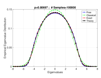
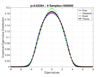
Figure 6: Sum of a diagonal random matrix with normally distributed diagonal entries with a block diagonal matrix whose diagonal blocks are independently drawn from the $\ell\times\ell$ GOE. Left: $\ell=8$ and Right: $\ell=4$. In each sample we generate new matrices. Compare the empirical $p$ values on the plots with the theoretical that one obtains from Eq. (35), which for $\ell=8$ is $p=0.8048$ and for $\ell=4$ is $p=0.62264$.

$$M_{2}=\left[\begin{array}[]{cccc}B_{1}\\ &B_{2}\\ &&\ddots\\ &&&B_{k}\end{array}\right]$$ (34)

where each $B_{k}$ is an $\ell\times\ell$ independent GOE matrix with $k\ell=m$ (see Fig. (6)). We illustrate the technique with $a_{i}\sim{\cal N}(0,1)$. In Fig. (6) we plot the eigenvalue distribution based on samples of $M_{1}$ and $M_{2}$ as indicated on the plots for $\ell=8$ and $\ell=4$. Numerically, in each sample we obtain each $B_{i}$ by first generating an $\ell\times\ell$ random real gaussian matrix $G_{i}$, whose entries are standard normals and then define $B_{i}$

$$B_{i}=\frac{G_{i}^{T}+G_{i}}{2}.$$

This is an example for which the relative eigenvectors have a block-diagonal structure and therefore do not satisfy the uniformity property in Assumption (1).

Below we derive formulas for general matrices of size $m$ with $k$ blocks of size $\ell\times\ell$ (clearly $k\ell=m$) and for general $\beta$.

From the above, and using the fact that $M_{1}$ and $M_{2}$ are independent, it is easy to see that $\mathbb{E}\text{Tr}[M_{1}^{2}M_{2}^{2}]=\sum_{i,j}\mathbb{E}(\lambda_{i}^{2})\mathbb{E}(|b_{ij}|^{2})$. If $\lambda_{i}\sim{\cal N}(0,1)$, then $\mathbb{E}(\lambda_{i}^{2})=1$ for all $i$. Moreover, since the total number of nonzero diagonal terms in $B$ is $m$ and the total number of nonzero diagonal terms is $k\ell(\ell-1)=m(\ell-1)$ we have

$$\mathbb{E}(|b_{ij}|^{2}) = \frac{1}{m^{2}}\sum_{i,j}|b_{ij}|^{2}=\frac{1}{m^{2}}\left\{m\mathbb{E}(b_{11}^{2})+m(\ell-1)\mathbb{E}(|b_{12}|^{2})\right\}$$

$$= \frac{1}{m}\left[1+\left(\ell-1\right)\frac{\beta}{2}\right]\qquad\text{For G(O/U/S)E block-diag. matrix}.$$

because for the G(O/U/S)E matrix, the variance of any diagonal entry is clearly $1$ and any off diagonal entry is $\beta/2$. Therefore the classical answer is $\mathbb{E}\text{Tr}[M_{1}^{2}M_{2}^{2}]=\sum_{i,j}\mathbb{E}(|b_{ij}|^{2})=m\left(1+\beta(\ell-1)/2\right)$.

Let us now calculate, the exact departing term. By the independence of $M_{1}$ and $M_{2}$ and since $\mathbb{E}(\lambda_{i}\lambda_{j})=\delta_{i,j}\mathbb{E}(\lambda_{i}^{2})$, we have $\mathbb{E}\text{Tr}[(M_{1}M_{2})^{2}]=\mathbb{E}\sum_{i,j}\lambda_{i}\lambda_{j}|b_{ij}|^{2}=k\mathbb{E}\sum_{1\leq i,j\leq\ell}\lambda_{i}\lambda_{j}|b_{ij}|^{2}=k\left\{\ell\mathbb{E}(\lambda_{i}^{2})\mathbb{E}(|b_{ii}|^{2})\delta_{i,j}\right\}=k\ell=m$.

We now turn to the corresponding quantity in the free approximation. In the formulas above (Eq. (33)) we need $\mathbb{E}(\mu_{i})$ , $\mathbb{E}(\mu_{i}\mu_{j})$ and $\mathbb{E}(\mu_{i}^{2})$, where now $\mu_{i}$ denotes an eigenvalue. For the G(O/U/S)E, $\mathbb{E}(\lambda_{i})=0$. Denoting by $||\centerdot||_{F}$ the Frobenius norm, for any $\ell\times\ell$ G(O/U/S)E matrix $B_{k}$ we have $\mathbb{E}(\mu_{i}^{2})=\frac{1}{\ell}\mathbb{E}||B_{k}||_{F}$, but $||B_{k}||_{F}=\frac{1}{\ell}\mathbb{E}\left\{\sum_{1\leq i,j\leq\ell}|b_{i,j}|^{2}\right\}=\frac{1}{\ell}\{\ell\mathbb{E}(|b_{i,i}|^{2}+\ell(\ell-1)\mathbb{E}(|b_{i,j}|^{2})\}$. We conclude that $\mathbb{E}(\mu_{i}^{2})=\left(1+\beta(\ell-1)/2\right)$. However, the size of $Q_{\beta}$ matrix is still $m$. To calculate $\mathbb{E}(\mu_{i}\mu_{j})$ for $j\neq i$ note that

$$\mathbb{E}[\text{Tr}(B_{k})\text{Tr}(B_{k})]=\mathbb{E}\sum_{i=1}^{\ell}\mu_{i}^{2}+\mathbb{E}\sum_{i\neq j}\mu_{i}\mu_{j}$$

But $X_{\ell}\equiv\text{Tr}(B_{k})$ is a sum of $\ell$ independent standard normal variables, which has mean zero and variance $\ell$. Moreover, by independence and zero mean, the cross terms are zero and we have $\mathbb{E}[\text{Tr}(B_{k})\text{Tr}(B_{k})]=\mathbb{E}[X_{\ell}^{2}]=\ell$. Lastly, we just derived $\mathbb{E}(\mu_{i}^{2})$, so we have

$$\mathbb{E}(\mu_{i}^{2}) = 1+\frac{\beta(\ell-1)}{2},$$

$$\mathbb{E}\sum_{i\neq j}\mu_{i}\mu_{j} = \ell(\ell-1)\beta/2\implies\mathbb{E}(\mu_{i}\mu_{j})=-\frac{\beta}{2}.\qquad\text{For G(O/U/S)E}$$

Comment: For $\mathbb{E}(\mu_{i}\mu_{j})$ the size of the matrix and its blocks are irrelevant.

Because of independence of $M_{1}$ from $M_{2}$ and $\mathbb{E}(\lambda_{i}\lambda_{j})=\delta_{i,j}$, the first and third sums in Eq. (33) vanish. Moreover by the independence of eigenvalues from eigenvectors the expectation is taken term-wise as

$$\mathbb{E}\text{Tr}\left[\left(M_{1}Q_{\beta}^{\dagger}\Lambda_{2}Q_{\beta}\right)^{2}\right] = \frac{\beta}{(m\beta+2)}\sum_{j\neq p}\text{ }\mathbb{E}(\mu_{j}\mu_{p})+\frac{\beta+2}{(m\beta+2)}\sum_{j}\mathbb{E}(\mu_{j}^{2})$$

$$= \frac{m(\ell\beta+2)}{m\beta+2},$$

because $\sum_{j\neq p}\mathbb{E}(\mu_{j}\mu_{p})=k\sum_{1\leq j\neq p\leq\ell}\mathbb{E}(\mu_{j}\mu_{p})$ and Weingarten formulas (see Eq. (13) and the Table below it).

Comment: The analytically derived values for $\mathbb{E}(|b_{ij}|^{2})$, $\mathbb{E}(\mu_{i}\mu_{j})$, $\mathbb{E}(\mu_{j}^{2})$, and $\mathbb{E}\text{Tr}\left[\left(M_{1}Q_{\beta}^{\dagger}\Lambda_{2}Q_{\beta}\right)^{2}\right]$ were all checked against numerics with high accuracy.

We can now analytically obtain $p$ (Eq. (32)) for this problem to be

$$p=\frac{(\ell-1)(m\beta+2)}{(\ell-1)(m\beta+2)+2(m-\ell)}.$$ (35)

Remark 7.

Note that when $\ell=m$, $p=1$ as expected the free answer becomes exact when one sums a random diagonal matrix with an $m\times m$ G(O/U/S)E. Also note the remarkable agreement of theoretical (Eq. (35)) and empirical $p$ values in Fig. (6)

If we were to use Eq. (20) we would obtain for the example in this section $p=1-m\mathbb{E}[|q_{s}|^{4}]=(\ell-1)/(\ell+2)$. The reason there is a discrepancy with Eq. (35) is that the block diagonal matrix $M_{2}$ does not obey Assumption (1).

VI.2 Sum of a diagonal with fixed Kac-Mudrock-Szego or Laplacian matrix

Next we take the diagonal entries of $M_{1}$ to be $a_{i}\in[-1,+1]$ and take $M_{2}=K$, where $Q$ is a Haar orthogonal matrix and $K$ is the Kac-Mudrock-Szego matrix, whose entries, denoted by $k_{i,j}$, are

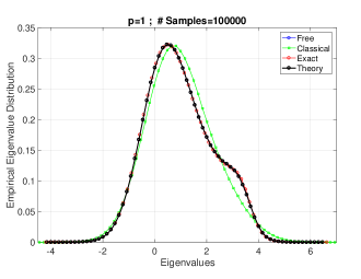
Figure 7: Sum of a diagonal random matrix, $M_{1}$, with standard normal entries and the matrix, $M_{2}=Q^{T}KQ$, where $K$ is taken to be Kac-Mudrock-Szego. Note that the eigenvalues of $M_{2}$ are fixed.

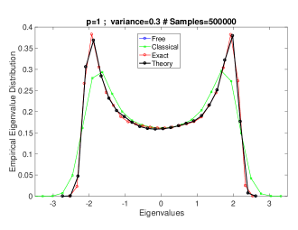
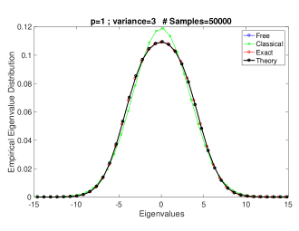
Figure 8: Left: (Anderson model) with variance $\text{var}(\lambda_{i})=0.3$. Sum of a diagonal random gaussian matrix, $M_{1}$, and the hopping matrix, $M_{2}=Q^{T}(2\mathbb{I}+L)Q$, where $L$ is the Laplacian matrix. Right: (Anderson model) with $\text{var}(\lambda_{i})=3$. Note that in all these plots examples $M_{2}$ has a fully deterministic set of eigenvalues. In Fig. (2) we show the case where $\text{var}(\lambda_{i})=1$.

$$k_{ij}=\rho^{|i-j|}$$

where we take $\rho=1/2$; it can be shown that when $0<\rho<1$ then $M_{2}\geq 0$. We show the eigenvalues of the sum in Fig. (7).

Lastly, we illustrate how well the density of states of the Anderson model is captured by this technique. In this case $M_{1}=\text{diag}(a_{1},\dots,a_{n})$, where $a_{i}$’s are independent standard gaussians and $M_{2}$ is the nearest neighbors hopping matrix with periodic boundary conditions

$$M_{2}=\left[\begin{array}[]{ccccc}0&1&&&1\\ 1&0&1\\ &1&0&\ddots\\ &&\ddots&\ddots&1\\ 1&&&1&0\end{array}\right].$$

$M_{2}$ is equal to a shifted Laplacian matrix, where $M_{2}=2\mathbb{I}+L$, where $\mathbb{I}$ is the identity and $L$ is the Laplacian matrix. Elsewhere, we took $a_{i}$ to be randomly distributed from the semi-circle law and proved that $M_{1}$ and $M_{2}$ have moments matching up to $8$ chen2012error . We showed that the method is successful across the range of the strength of disorder (see Fig. (2) and Fig. (8)). Like in there we find that the free approximation alone is quite adequate.

Comment: If one sets to find $p$ numerically by matching fourth moments, one should note that the kurtosis can be very slow to converge. In principle, if two matrices are free, one could numerically observe a $p>1$ or if the classical end is the exact theory then $p<0$ can be observed. These are byproducts of numerical inaccuracies of computing the kurtoses.

VII An Application: Density of State of Generic Local Quantum Spin Chains

The density of states encodes useful information about the physics of many-body systems. Here we apply our technique to quantum many-body systems with generic interactions movassagh2011density ; movassagh_IE2010 . Consider the Hamiltonian acting on the joint Hilbert space of $n$ $d-$dimensional complex vector spaces (e.g., spin $s$ particles, where $d=2s+1$). The joint Hilbert space is $\left(\mathbb{C}^{d}\right)^{\otimes n}$ and the nearest neighbor interactions is given by the Hamiltonian

$$H=\sum_{k=1}^{n-1}\mathbb{I}_{d^{k-1}}\otimes H_{k,k+1}\otimes\mathbb{I}_{d^{n-k-1}}$$ (36)

where each $H_{k,k+1}$ is a $d^{2}\times d^{2}$ matrix that we take to be generic. For example, the local interactions can be distributed according to GUE, or be random projectors, or Wishart matrices etc.

The problem statement is then: Suppose the eigenvalue distribution of $H_{k,k+1}$ is known, what is the eigenvalue distribution of $H$?

The exact problem is NP-Complete brown2011computational . There are two main sources of difficulties: 1. The size of the matrix $H$ is $d^{n}\times d^{n}$, which makes the exact diagonalization difficult even for moderate sized problems. 2. Any two consecutive terms in Eq. (36) do not commute.

Despite these challenges and the NP-completeness of the exact result, the method described above provides an excellent approximation to the true distribution. We now proceed to detail the results corroborated with various numerical illustrations.

In Eq. (36) the summands with $k$ odd all commute. Similarly the summands with $k$ even all commute. This enables us to write $H$ in Eq. (36) as

$$H_{odd}+H_{even},$$ (37)

where each $H_{odd}$ and $H_{even}$ is $d^{n}$ dimensional and is given by

$$H_{odd} = \sum_{k\text{ odd}}\mathbb{I}_{d^{k-1}}\otimes H_{k,k+1}\otimes\mathbb{I}_{d^{n-k-1}},$$

$$H_{even} = \sum_{k\text{ even}}\mathbb{I}_{d^{k-1}}\otimes H_{k,k+1}\otimes\mathbb{I}_{d^{n-k-1}}.$$

We take $H_{odd}$ and $H_{even}$ as our two known matrices, where an eigenvalue decomposition gives

$$H_{odd} =U_{odd}^{\dagger}\Lambda_{odd}U_{odd}$$

$$H_{even} =U_{even}^{\dagger}\Lambda_{even}U_{even}.$$

The unitary matrices of eigenvectors, $U_{odd}$ and $U_{even}$, are (for an odd sized chain)

$$U_{odd} = U_{1,2}\otimes U_{3,4}\otimes\cdots\otimes U_{n-2,n-1}\otimes\mathbb{I}_{d}$$

$$U_{even} = \mathbb{I}_{d}\otimes U_{2,3}\otimes U_{4,5}\otimes\cdots\otimes U_{n-1,n}.$$

In these equations $U_{k,k+1}$ denotes the eigenvector matrix of $H_{k,k+1}$ and is therefore $d^{2}\times d^{2}$ in size.

The diagonal real matrices of eigenvalues $\Lambda_{odd}$ and $\Lambda_{even}$ are

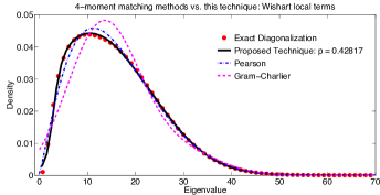
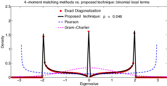
Figure 9: Comparison of our technique with Gram-Charlier and Beta-ensemble. The left corresponds to what was shown in Fig. (2) and the right is a spin chain of length $3$ where each of the two local interactions has Haar eigenvectors and Bernoulli $\pm 1$ eigenvalues. In the latter, we took the size of each local term to be $25\times 25$; therefore $H$ is $125\times 125$.

$$\Lambda_{odd} =\sum_{k\text{ odd}}\mathbb{I}_{d^{k-1}}\otimes\Lambda_{k,k+1}\otimes\mathbb{I}_{d^{n-k-1}},$$

$$\Lambda_{even} =\sum_{k\text{ even}}\mathbb{I}_{d^{k-1}}\otimes\Lambda_{k,k+1}\otimes\mathbb{I}_{d^{n-k-1}},$$

and $\Lambda_{k,k+1}$ is the real and diagonal matrix of the eigenvalues of $H_{k,k+1}$. The eigenvalues of $\Lambda_{odd}$ corresponds to all possible sums of the eigenvalues of $\Lambda_{k,k+1}$, which is easy to obtain. Similarly $\Lambda_{even}$ is easy to compute.

With no loss of generality we change basis in which $H_{odd}$ is diagonal, whereby we have

$$H=\Lambda_{odd}+Q_{s}^{-1}\Lambda_{even}Q_{s}$$

and $Q_{s}\equiv U_{odd}U_{even}^{\dagger}$. The problem then is to find a good approximation for the density of states of $H$. Recall that we have two extreme ends that correspond to the classical and free approximations

$$H_{c} =\Lambda_{odd}+\Pi^{-1}\Lambda_{even}\Pi$$

$$H_{f} =\Lambda_{odd}+Q^{-1}\Lambda_{even}Q$$

where $\Pi$ and $Q$ are permutation and $\beta-$orthogonal Haar matrices respectively (exactly as before). In the left figure of Fig. (2) we showed the DOS for $H$, $H_{c}$ , $H_{f}$ and the proposed technique; the convex combination parameter here is $p=0.43$.

How does our technique compare to other known techniques? To the best of our knowledge there are two note-worthy techniques that we can compare against. The first is the Gram-Charlier expansion cramer2016mathematical which builds the distribution from the knowledge of first $k$ moments. The second is a fit to the beta-distribution, which is part of MatLab’s library of function (pearson.m). Our technique, unlike the others, seems to work much better than what one would expect from the knowledge of the first four moments alone.

VIII Discussions: Limitations and Comparison

In this paper we described a technique for calculating the eigenvalue distribution of sums of matrices from the knowledge of the distribution of the summands. The input to the theory is the known distribution of the summands and the output is an approximation to the density of the sum. We have laid out a step by step technology by which such calculations can be carried out and provided an eigenvalue finding subroutine which circumvents solving high order polynomials to solve for the complex roots needed. We then compared our theory against exact diagonalization. Through our numerical work we find that the theory proposed gives excellent approximation of the exact eigenvalue distributions in most cases.

The technique described above outputs an eigenvalue distribution, which is a continuous curve or union of continuous curves. It is limited in that it does not provide level spacing statistics (for $M$ in Eq. (1)). For many problems of interest in physics, such as quantum many-body systems, the difference between the smallest two eigenvalues is of utmost importance. This difference is simply called the gap. Elsewhere we have proved that there is a continuum of eigenvalues above the smallest eigenvalue movassagh2016generic . Although this implies that the gap tends to zero as $m\rightarrow\infty$ for generic (local) interactions and that we can quantify how it goes to zero for gaussian ensembles, we do not have a detailed enough description of eigenvalue spacings beyond.

Density of states does not necessarily provide information about 2-point or higher order correlation functions. It would be interesting if they were investigated.

We are aware of two other works (benaych2011continuous and bozejko1997q ) that formulate some form of interpolation between a “free” object and a “classical” object: In benaych2011continuous , a random unitary matrix is explicitly constructed through a Brownian motion process starting at time $t=0$, and going to time $t=\infty$. “Classical” corresponds to $t=0$, and “free” corresponds to $t=\infty$. The random unitary matrix starts non-random and is randomized continuously until it fully reaches Haar measure. In bozejko1997q , through detailed combinatorial constructions and investigation into Fock space representations of Fermions and Bosons, unique measures are constructed that interpolate between the limit of the classical central limit theorem, the gaussian, and the free central limit theorem, the semicircle. The curve also continues on to $t=-1$, which corresponds to two non-random atoms.

An unknown question is whether the unitary construction in benaych2011continuous leads to the same convolution interpolate as this paper where we take a convex combination. Another unknown question is whether our proposal and benaych2011continuous lead to an analog of a limit of a central limit theorem which would match that of bozejko1997q .

We outline in the table below features found in each paper. The empty boxes are opportunities for further research.

	Application	Unitary Matrix Construction	Interpolate Convolution	Iterate Convolution to a CLT
This work	✔		✔
benaych2011continuous		✔	✔
bozejko1997q				✔

Lastly, this work proposes a technique to obtain the eigenvalue distribution. To ultimately understand the powers and limitations of it, it would be most useful to take an applied perspective and apply it to concrete problems.

IX Acknowledgements

Some of this work was completed while RM had the support of the Simons Foundation and the American Mathematical Society through the AMS-Simons travel grant, and IBM Research’s support and freedom offered by his former Herman Goldstine Fellowship. AE was supported by the National Science Foundation through the grant DMS-1312831.

References

- [1] Florent Benaych-Georges and Thierry Lévy. A continuous semigroup of notions of independence between the classical and the free one. The Annals of Probability, pages 904–938, 2011.
- [2] Marek Bożejko, Burkhard Kümmerer, and Roland Speicher. q-gaussian processes: non-commutative and classical aspects. Communications in Mathematical Physics, 185(1):129–154, 1997.
- [3] Brielin Brown, Steven T Flammia, and Norbert Schuch. Computational difficulty of computing the density of states. Physical review letters, 107(4):040501, 2011.
- [4] Jiahao Chen, Eric Hontz, Jeremy Moix, Matthew Welborn, Troy Van Voorhis, Alberto Suárez, Ramis Movassagh, Alan Edelman, et al. Error analysis of free probability approximations to the density of states of disordered systems. Physical review letters, 109(3):036403, 2012.
- [5] Harald Cramér. Mathematical Methods of Statistics (PMS-9), volume 9. Princeton university press, 2016.
- [6] Alfred Horn. Eigenvalues of sums of hermitian matrices. Pacific Journal of Mathematics, 12(1):225–241, 1962.
- [7] Alexander A Klyachko. Stable bundles, representation theory and hermitian operators. Selecta Mathematica, New Series, 4(3):419–445, 1998.
- [8] Allen Knutson and Terence Tao. Honeycombs and sums of hermitian matrices. Notices Amer. Math. Soc, 48(2), 2001.
- [9] R Movassagh and A Edelman. Isotropic entanglement.(2010). arXiv preprint arXiv:1012.5039.
- [10] Ramis Movassagh. Generic local hamiltonians are gapless. arXiv preprint arXiv:1606.09313, 2016.
- [11] Ramis Movassagh and Alan Edelman. Density of states of quantum spin systems from isotropic entanglement. Physical review letters, 107(9):097205, 2011.
- [12] Alexandru Nica and Roland Speicher. Lectures on the combinatorics of free probability, volume 13. Cambridge University Press, 2006.
- [13] Sheehan Olver and Raj Rao Nadakuditi. Numerical computation of convolutions in free probability theory. arXiv preprint arXiv:1203.1958, 2012.
- [14] John Riordan. Introduction to combinatorial analysis. Courier Corporation, 2012.
- [15] Lloyd N Trefethen and David Bau III. Numerical linear algebra, volume 50. Siam, 1997.
- [16] Dan V Voiculescu, Ken J Dykema, and Alexandru Nica. Free random variables. Number 1. American Mathematical Soc., 1992.
- [17] Hermann Weyl. Das asymptotische verteilungsgesetz der eigenwerte linearer partieller differentialgleichungen (mit einer anwendung auf die theorie der hohlraumstrahlung). Mathematische Annalen, 71(4):441–479, 1912.