Does the Galaxy-Halo Connection Vary with Environment?

Abstract

SubHalo Abundance Matching (SHAM) assumes that one (sub)halo property, such as mass $M_{\rm vir}$ or peak circular velocity $V_{\rm peak}$, determines properties of the galaxy hosted in each (sub)halo such as its luminosity or stellar mass. This assumption implies that the dependence of Galaxy Luminosity Functions (GLFs) and the Galaxy Stellar Mass Function (GSMF) on environmental density is determined by the corresponding halo density dependence. In this paper, we test this by determining from an SDSS sample the observed dependence with environmental density of the $ugriz$ GLFs and GSMF for all galaxies, and for central and satellite galaxies separately. We then show that the SHAM predictions are in remarkable agreement with these observations, even when the galaxy population is divided between central and satellite galaxies. However, we show that SHAM fails to reproduce the correct dependence between environmental density and $g-r$ color for all galaxies and central galaxies, although it better reproduces the color dependence on environmental density of satellite galaxies.

1 Introduction

In the standard theory of galaxy formation in a $\Lambda$CDM universe, galaxies form and evolve in massive dark matter halos. The formation of dark matter halos is through two main mechanisms: (1) the accretion of diffuse material, and (2) the incorporation of material when halos merge. At the same time, galaxies evolve within these halos, where multiple physical mechanisms regulate star formation and thus produce their observed properties. Naturally, this scenario predicts that galaxy properties are influenced by the formation and evolution of their host halos (for a recent review see Somerville & Davé, 2015).

What halo properties matter for galaxy formation? The simplest assumption that galaxy formation models make is that a dark matter halo property such as mass $M_{\rm vir}$ or maximum circular velocity $V_{\rm max}$ fully determines the statistical properties of their host galaxies. This assumption was supported by early studies that showed that the halo properties strongly correlate with the larger-scale environment mainly due to changes in halo mass (e.g., Lemson & Kauffmann, 1999). Halo evolution and corresponding evolution of galaxy properties can be predicted from Extended Press-Schechter analytical models based on Monte Carlo merger trees (Cole, 1991; White & Frenk, 1991; Kauffmann & White, 1993; Somerville & Kolatt, 1999). Such models assume that the galaxy assembly time and merger history are independent of the large-scale environment (for a recent discussion see, e.g., Jiang & van den Bosch, 2014).

However, it is known that dark matter halo properties do depend on other aspects beyond $M_{\rm vir}$, a phenomenon known as halo assembly bias. Wechsler et al. (2006, see also , ) observed an assembly bias effect in the clustering of dark matter halos: they showed that for halos with $\mbox{$M_{\rm vir}$}\lower 2.15277pt\hbox{$\;\buildrel<\over{\sim}\;$}10^{13}\mbox{M${}_{\odot}$}$ early forming halos are more clustered than late forming halos, while for more massive halos they found the opposite. Other effects of environmental density on dark matter halos are known, for example that halo mass accretion rates and spin can be significantly reduced in dense environments due to tidal effects, and that median halo spin is significantly reduced in low-density regions due to the lack of tidal forces there (Lee et al., 2017). Indeed there are some recent efforts to study assembly bias and the effect of the environment on the galaxy-halo connection in the context of galaxy clustering (Lehmann et al., 2017; Vakili & Hahn, 2016; Zentner et al., 2016; Zehavi et al., 2017) and weak lensing (Zu et al., 2017). Despite such environmental effects on halo properties, it may still be true that some galaxy properties can be correctly predicted from just halo $M_{\rm vir}$ or $V_{\rm max}$.

The assumption that dark matter halo mass fully determines the statistical properties of the galaxies that they host has also influenced the development of empirical approaches for connecting galaxies to their host halo: the so-called halo occupation distribution (HOD) models (Berlind & Weinberg, 2002) and the closely related conditional stellar mass/luminosity function model (Yang, Mo & van den Bosch, 2003; Cooray, 2006). HOD models assume that the distribution of galaxies depends on halo mass only (Mo et al., 2004; Abbas & Sheth, 2006). Yet the HOD assumption has been successfully applied to explain the clustering properties of galaxies not only as a function of their mass/luminosity only but also as a function of galaxy colors (Jing, Mo & Börner, 1998; Berlind & Weinberg, 2002; Zehavi et al., 2005; Zheng et al., 2005; Tinker et al., 2013; Rodríguez-Puebla et al., 2015).

The (sub)halo abundance matching (SHAM) approach takes the above assumption to the next level by assuming that not only does a halo property, such as mass $M_{\rm vir}$ or maximum circular velocity $V_{\rm max}$, determine the luminosity or stellar mass of central galaxies, but also that there is a simple relation between subhalo properties and those of the satellite galaxies they host. Specifically, we will assume that subhalo peak circular velocity $V_{\rm peak}$ fully determines the corresponding properties of their hosted satellite galaxies (Reddick et al., 2013). For simplicity, in the remainder of this paper, when we write $V_{\rm max}$ we will mean the maximum circular velocity for distinct halos, and the peak circular velocity of subhalos. SHAM assigns by rank a halo property, such as $V_{\rm max}$, to that of a galaxy property, such as luminosity or stellar mass, by matching their corresponding cumulative number densities (Kravtsov et al., 2004; Vale & Ostriker, 2004; Conroy, Wechsler & Kravtsov, 2006; Conroy & Wechsler, 2009; Behroozi, Conroy & Wechsler, 2010; Behroozi, Wechsler & Conroy, 2013; Moster, Naab & White, 2013, 2017; Rodríguez-Puebla et al., 2017).

While central galaxies are continuously growing by in-situ star formation and/or galaxy mergers, satellite galaxies are subject to environmental effects such as tidal and ram-pressure stripping, in addition to interactions with other galaxies in the halo and with the halo itself. Therefore, central and satellite galaxies are expected to differ in the relationship between their host halos and subhalos (see e.g., Neistein et al., 2011; Rodríguez-Puebla, Drory & Avila-Reese, 2012; Yang et al., 2012; Rodríguez-Puebla, Avila-Reese & Drory, 2013). Nevertheless, SHAM assumes that (sub)halo $V_{\rm max}$ fully determines the statistical properties of the galaxies. Thus SHAM galaxy properties evolve identically for central and satellite galaxies, except that satellite galaxy properties are fixed after $V_{\rm peak}$ is reached. SHAM also implies that galaxy properties are independent of local as well as large-scale environmental densities. Thus two halos with identical $V_{\rm max}$ but in different environments will host identical galaxies. Despite the extreme simplicity of this approach, the two point correlation functions predicted by SHAM are in excellent agreement with observations (Reddick et al., 2013; Campbell et al., 2017, and Figures 4 and 5 below), showing that on average galaxy clustering depends on halo $V_{\rm peak}$. It is worth mentioning that neither HOD nor SHAM identify clearly which galaxy property, luminosity in various wavebands or stellar mass, depends more strongly on halo mass—although, theoretically, stellar mass growth is expected to be more closely related to halo mass accretion (Rodríguez-Puebla et al., 2016b).

Our main goal in this paper is to determine whether the assumption that one (sub)halo property, in our case halo $V_{\rm max}$ and subhalo $V_{\rm peak}$, fully determines some statistical properties of the hosted galaxies. This might be true even though the galaxy-halo relation is expected to depend on environment because the properties of the galaxies might reflect halo properties that depend on some environmental factor (see e.g., Lee et al., 2017). We will test this assumption by determining from a Sloan Digital Sky Survey (SDSS) sample the dependence on environmental density of the $ugriz$ galaxy luminosity functions (GLFs) as well as the Galaxy Stellar Mass Function (GSMF) for all galaxies, and separately for central and satellite galaxies, and comparing these observational results with SHAM predictions. We will also investigate which of these galaxy properties is better predicted by SHAM. If a galaxy-halo connection that is independent of environment successfully reproduces observations in the nearby universe, then we can conclude that the relation may be appropriate to use for acquiring other information about galaxies. It also suggests that this assumption be tested at larger redshifts. To the extent that the galaxy-halo connection is independent of density or other environmental factors, it is a great simplification.

This paper is organized as follows. In Section 2, we describe the galaxy sample that we utilize for the determination of the environmental dependence of the $ugriz$ GLFs and GSMF. Section 3 describes our mock galaxy catalog based on the Bolshoi-Planck cosmological simulation. Here we show how SHAM assigns to every halo in the simulation has five band magnitudes, $ugriz$, and a stellar mass. In Section 4, we present the dependence with environment of $ugriz$ GLFs and GSMF both for observations and for SHAM applied to the Bolshoi-Planck simulation. We show that the SHAM predictions are in remarkable agreement with observations even when the galaxy population is divided between central and satellite galaxies. However, we also find that SHAM fails to reproduce the correct dependence between environmental density and $g-r$ color. Finally Section 5 summarizes our results and discusses our findings. We adopt a Chabrier (2003) IMF and the Planck cosmological parameters used in the Bolshoi-Planck simulation: $\Omega_{\Lambda}=0.693,\Omega_{\rm M}=0.307,h=0.678$.

2 Observational Data

In this section we describe the galaxy sample that we utilize for the determination of the galaxy distribution. We use the standard 1/$\mathcal{V}_{\rm max}$ weighting procedure for the determination of the $ugriz$ Galaxy Luminosity Functions (GLFs) and the Galaxy Stellar Mass Function (GSMF) and report their corresponding best fitting models. We show that a function composed of a single Schechter function plus another Schechter function with a sub-exponential decreasing slope is an accurate model for the $ugriz$ GLFs as well as the GSMF. Finally, we describe the methodology for the determination of the environmental density dependence of the $ugriz$ GLFs and GSMF.

2.1 The Sample of Galaxies

In this paper we utilize the New York Value Added Galaxy Catalog NYU-VAGC (Blanton et al., 2005b) based on the the SDSS DR7. Specifically, we use the large galaxy group catalog from Yang et al. (2012) with $\sim 6\times 10^{5}$ spectroscopic galaxies over a solid angle of $7748$ deg² comprising the redshift range $0.01<z<0.2$ with an apparent magnitude limit of $m_{{\rm lim},r}=17.77$. However, the sample we use in this paper is $0.03<z<0.11$ (see Figure 2 below).

The Yang et al. (2012) catalog is a large halo-based galaxy group catalog that assigns group membership by assuming that the distribution of galaxies in phase space follows that of dark matter particles. Mock galaxy catalogs demonstrate that $\sim 80\%$ of all their groups have a completeness larger than $80\%$ while halo groups with mass $M_{\rm vir}>10^{12.5}h^{-1}\mbox{M${}_{\odot}$}$ have a completeness $>95\%$; for more details see Yang et al. (2007). Here, we define central galaxies as the most massive galaxy in their group in terms of stellar mass; the remaining galaxies will be regarded as satellites.

The definition of groups in the Yang et al. (2012) catalog is very broad and includes systems that are often explored individually in the literature, such as clusters, compact groups, fossil groups, rich groups, etc. That is, this galaxy group catalog is not biased to a specific type of group. Instead, this galaxy group catalog is diverse and, more importantly, closely related to the general idea of galaxy group that naturally emerges in the $\Lambda$CDM paradigm: that halos host a certain number of galaxies inside their virial radius. Therefore, the Yang et al. (2012) galaxy group catalog is ideal for comparing to predictions based on $N$-body cosmological simulations. For the purpose of exploring whether certain galaxy properties are fully determined by the (sub)halo in which they reside, this galaxy group catalog will help us to draw conclusions not only at the level of the global GLFs and GSMF but also at the level of centrals and satellites. Thus, the Yang et al. (2012) galaxy group catalog is an ideal tool to explore at a deeper level the simple assumptions in the SHAM approach.

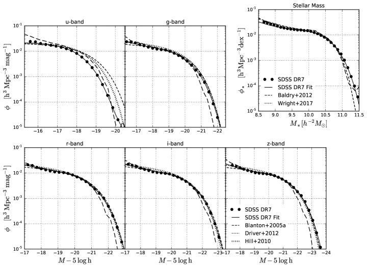
Figure 1: The global $ugriz$ galaxy luminosity function. Our derived $ugriz$ GLFs and GSMF are shown with the black circles with error bars. For comparison we reproduce the $ugriz$ GLFs from Blanton et al. (2005a, black long dashed lines) based on the SDSS DR2; Hill et al. (2010, dotted lines) by combining the MGC, SDSS DR5 and the UKIDSS surveys; and Driver et al. (2012, short dashed lines) based on the GAMA survey. As for the stellar masses we compare with the GSMF from Baldry et al. (2012) and Wright et al. (2017), black long and short dashed lines, respectively.

Table 1: Best fitting parameters for the GLFs and the GSMF.

Galaxy Luminosity Functions
Band	$\alpha$	$M^{*}-5\log h$	$\log\phi^{*}_{1}$ $\left[h^{3}{\rm Mpc}^{-3}{\rm mag}^{-1}\right]$	$\log\phi_{2}^{*}$ $\left[h^{3}{\rm Mpc}^{-3}{\rm mag}^{-1}\right]$	$\beta$
$u$	$-0.939\pm 0.005$	$-17.758\pm 0.016$	$-1.530\pm 0.002$	$-3.692\pm 0.044$	$0.721\pm 0.008$
$g$	$-1.797\pm 0.044$	$-19.407\pm 0.068$	$-2.764\pm 0.105$	$-1.674\pm 0.013$	$0.821\pm 0.014$
$r$	$-1.810\pm 0.036$	$-20.184\pm 0.062$	$-2.889\pm 0.094$	$-1.733\pm 0.013$	$0.813\pm 0.013$
$i$	$-1.794\pm 0.031$	$-20.546\pm 0.053$	$-2.896\pm 0.077$	$-1.768\pm 0.011$	$0.815\pm 0.011$
$z$	$-1.816\pm 0.028$	$-20.962\pm 0.051$	$-3.038\pm 0.076$	$-1.806\pm 0.012$	$0.827\pm 0.011$
Galaxy Stellar Mass Function
	$\alpha$	$\mathcal{M}^{*}$ $\left[h^{-2}\mbox{M${}_{\odot}$}\right]$	$\log\phi^{*}_{1}$ $\left[h^{3}{\rm Mpc}^{-3}{\rm dex}^{-1}\right]$	$\log\phi_{2}^{*}$ $\left[h^{3}{\rm Mpc}^{-3}{\rm dex}^{-1}\right]$	$\beta$
	$-1.664\pm 0.033$	$10.199\pm 0.0303$	$-3.041\pm 0.082$	$-1.885\pm 0.010$	$0.708\pm 0.012$

In order to allow for meaningful comparison between galaxies at different redshifts, we utilize model magnitudes that are K+E-corrected at the rest-frame $z=0$. These corrections account for the broad band shift with respect to the rest-frame broad band and for the luminosity evolution. For the K-corrections we utilize the input values tabulated in the NYU-VAGC catalog (Blanton & Roweis, 2007, corresponding to the kcorrect software version v$4\_1\_4$), while for the evolution term we assume a model given by

$$E_{j}(z)=-Q_{X}\times z,$$ (1)

where the subscript $X$ refers to the $u$, $g$, $r$, $i$ and $z$ bands and their values are $(Q_{u},Q_{g},Q_{r},Q_{i},Q_{z})=(4.22,1.3,1.1,1.09,0.76)$. Here we ignore potential dependences between $Q_{X}$ and colors (but see Loveday et al., 2012, for a discussion) and luminosity, and use global values only. Although this is a crude approximation for accounting for the evolution of the galaxies, it is accurate enough for our purposes since we are not dividing the galaxy distribution into subpopulations as a function of star formation rate and/or color.

We estimated the value of each $Q_{X}$ by determining first the $X$-band GLF when $Q_{X}=0$ at four redshift intervals: $[0.01,0.05]$, $[0.01,0.1]$, $[0.01,0.15]$ and $[0.01,0.2]$. When assuming $Q_{X}=0$, the GLFs are normally shifted towards higher luminosities, with this shift increasing with redshift. In other words, when ignoring the evolution correction, the GLF will result in an overestimation of the number density at higher luminosities and high redshifts. Thus, in order to account for this shift we find the best value for $Q_{X}$ that leaves the GLFs invariant at the four redshift intervals mentioned above. We note that our derived values are similar to those reported in Blanton et al. (2003). For the $u$-band we used the value reported in Blanton et al. (2003), but we have checked that the value of $Q_{u}=4.22$ also leaves the GLF invariant at the four redshifts bins mentioned above.

For stellar masses, we utilize the MPA-JHU DR7 database derived from photometry-spectral energy distribution fittings, explained in detail in Kauffmann et al. (2003). All stellar masses have been normalized to a Chabrier (2003) IMF and to the cosmology used for this paper.

2.2 The Global $ugriz$ Luminosity Functions and Stellar Mass Function

Next, we describe the procedure we utilize for determining the global GLFs and the GSMF.

Here, we choose the standard 1/$\mathcal{V}_{\rm max}$ weighting procedure for the determination of the $ugriz$ GLFs and the GSMF. Specifically, we determine the galaxy luminosity and stellar mass distributions as

$$\phi_{X}(M_{X})=\frac{1}{\Delta M_{X}}\sum_{i=1}^{N}\frac{\omega_{X}(M_{X}\pm\Delta M_{X}/2)}{\mbox{$\mathcal{V}_{{\rm max},i}$}},$$ (2)

where $M_{X}$ refers to $M_{u}$, $M_{g}$, $M_{r}$, $M_{i}$, $M_{z}$ and $\log\mbox{$M_{*}$}$, $\omega_{i}$ is the correction weight completeness factor in the NYU-VAGC for galaxies within the interval $M_{X}\pm\Delta M_{X}/2$, and

$$\mbox{$\mathcal{V}_{{\rm max},i}$}=\int_{\Omega}\int^{z_{u}}_{z_{l}}\frac{d^{2}V_{c}}{dzd\Omega}dzd\Omega.$$ (3)

We denote the solid angle of the SDSS DR7 with $\Omega$ while $V_{c}$ refers to the comoving volume enclosed within the redshift interval $[z_{l},z_{u}]$. The redshift limits are defined as $z_{l}={\rm max}(0.01,z_{\rm min})$ and $z_{u}={\rm min}(z_{\rm max},0.2)$; where $z_{\rm min}$ and $z_{\rm max}$ are, respectively, the minimum and maximum at which each galaxy can be observed in the SDSS DR7 sample. For the completeness limits, we use the limiting apparent magnitudes in the $r$-band of $r=14$ and $r=17.77$.

The filled black circles with error bars in Figure 1 present our determination of the global SDSS DR7 $ugriz$ GLFs. For comparison we reproduce the $ugriz$ GLFs from Blanton et al. (2005a, black long dashed line) who used a sample of low-redshift galaxies ($<150h^{-1}$Mpc) from the SDSS DR2 and corrected due to low surface brightness selection effects. Additionally, we compare to Hill et al. (2010) who combined data from the Millennium Galaxy Catalog (MGC), the SDSS DR5 and the UKIRT Infrared Deep Sky Survey Large Area Survey (UKIDSS) for galaxies with $z<0.1$, dotted lines; and to Driver et al. (2012) who utilized the Galaxy And Mass Assembly (GAMA) survey for the redshift interval $0.013<z<0.1$ to derive the $ugriz$ GLFs, short dashed-lines. All the GLFs in Figure 1 are at the rest-frame $z=0$. In general we observe good agreement with previous studies; in a more detailed examination, however, we note some differences that are worthwhile to clarify.

Consider the $u$-band GLFs from Figure 1 and note that there is an apparent tension with previous studies. At the high luminosity-end, our inferred $u$-band GLF decreases much faster than the above-mentioned studies. This is especially true when comparing with the Hill et al. (2010) and Driver et al. (2012) GLFs. This could be partly due to the differences between the Kron magnitudes used by Hill et al., 2010 and Driver et al., 2012 and the model magnitudes used in this paper. But we believe that most of the difference is due to the differences in the E-corrections, reflecting that our model evolution is more extreme than that of Hill et al. (2010) and Driver et al. (2012). This can be easily understood by noting that the high luminosity-end of the GLF is very sensitive to E-corrections. The reason is that brighter galaxies are expected to be observed more often at larger redshifts than fainter galaxies; thus Equation (1) will result in a small correction for lower luminosity galaxies (low redshift) but a larger correction for higher luminosity galaxies (high redshifts). Indeed, Driver et al. (2012) who did not determine corrections by evolution, derived a $u$-band GLF that predicts the largest abundance of high luminosity galaxies. On the other hand, the evolution model introduced by Hill et al. (2010) is shallower than ours, which results in a GLF between our determination and the Driver et al. (2012) $u$-band GLF. This could explain the apparent tension between the different studies. While the effects of evolution are significant in the $u$-band, they are smaller in the longer wavebands. Ideally, estimates of the evolution should be more physically motivated by galaxy formation models, but empirical measurements are more accessible and faster to determine; however, when making comparisons one should keep in mind that empirical estimates are by no means definitive.

Some previous studies have concluded that a single Schechter function is consistent with observations (see, e.g., Blanton et al., 2003, and recently Driver et al., 2012). However, other studies have found that a double Schechter function is a more accurate description of the GLFs (Blanton et al., 2005a). Additionally, recent studies have found shallower slopes at the high luminosity-end instead of an exponential decreasing slope in the GLFs (see e.g., Bernardi et al., 2010). In this paper, we choose to use GLFs that are described by a function composed of a single Schechter function plus another Schechter function with a subexponential decreasing slope for the $ugriz$ bands given by

$$\phi(M)=\frac{\ln 10}{2.5}\phi_{1}^{*}10^{0.4(M^{*}_{1}-M)\left(1+\alpha_{1}\right)}\exp\left(-10^{0.4\left(M^{*}_{1}-M\right)}\right)$$

$$+\frac{\ln 10}{2.5}\phi_{2}^{*}10^{0.4(M^{*}_{2}-M)\left(1+\alpha_{2}\right)}\exp\left(-10^{0.4\left(M^{*}_{2}-M\right)\beta}\right).$$ (4)

The units of the GLFs are $h^{3}$ Mpc^-3 mag^-1 while the input magnitudes have units of mag$-5\log h$. The parameters for the $ugriz$ bands are given in Table 1. Note that for simplicity we assume that $\alpha_{1}=\alpha$, $\alpha_{2}=1+\alpha$ and $M^{*}_{1}=M^{*}_{2}=M^{*}$. These assumptions reduce the number of free parameters to five. The corresponding best fitting models are shown in Figure 1 with the solid black lines. The filled circles with error bars in Figure 1 present our determinations for the global SDSS DR7 GLFs.

In the case of the GSMF, we compare our results with Baldry et al. (2012) and Wright et al. (2017) plotted with the black long and short dashed lines respectively. Both analyses used the GAMA survey to determine the local GSMF. Recall that our stellar masses were obtained from the MPA-JHU DR7 database. As can be seen in the figure, our determination is consistent with these previous results. We again choose to use a function composed of a single Schechter function plus another Schechter function with a subexponential decreasing slope for the GSMFgiven by

$$\phi_{*}(\mbox{$M_{*}$})=\phi_{1}^{*}{\ln 10}\left(\frac{\mbox{$M_{*}$}}{\mathcal{M}_{1}^{*}}\right)^{1+\alpha_{1}}\exp\left(-\frac{\mbox{$M_{*}$}}{\mathcal{M}_{1}^{*}}\right)$$

$$+\phi_{2}^{*}{\ln 10}\left(\frac{\mbox{$M_{*}$}}{\mathcal{M}_{2}^{*}}\right)^{1+\alpha_{2}}\exp\left[-\left(\frac{\mbox{$M_{*}$}}{\mathcal{M}_{2}^{*}}\right)^{\beta}\right].$$ (5)

The units for the GSMF are $h^{3}$ Mpc^-3 dex^-1 while the input stellar masses are in units of $h^{-2}\mbox{M${}_{\odot}$}$. Again, for simplicity we assume that $\alpha_{1}=\alpha$, $\alpha_{2}=1+\alpha$, and $\mathcal{M}_{1}^{*}=\mathcal{M}_{2}^{*}=\mathcal{M}^{*}$; again, this assumption reduces the number of free parameters to five. We report the best fitting value parameters in Table 1 and the corresponding best fitting model is presented with the solid black line in Figure 1. As we will describe in Section 3, we use the $ugriz$ GLFs and GSMF as inputs for our mock galaxy catalog.

2.3 Measurements of the Observed $ugriz$ GLFs and GSMF as a Function of Environment

Once we determined the global $ugriz$ GLFs and the GSMF, the next step in our program is to determine the observed dependence of the $ugriz$ GLFs and GSMF with environmental density.

2.3.1 Density-Defining Population

The SDSS DR7 limiting magnitude in the $r$-band is 17.77. Thus, in order to determine the local overdensity of each SDSS DR7 galaxy, we need to first construct a volume-limited density-defining population (DDP, Croton et al., 2005; Baldry et al., 2006). A volume-limited sample can be constructed by defining the minimum and maximum redshifts at which galaxies within some interval magnitude are detected in the survey. Following the McNaught-Roberts et al. (2014) GAMA paper, we define our volume-limited DDP sample of galaxies in the absolute magnitude range $-21.8<M_{r}-5\log h<-20.1$. A valid question is whether the definition utilized for the volume-limited DDP sample could lead to different results. This question has been studied in McNaught-Roberts et al. (2014); the authors conclude that the precise definition for the volume-limited DDP sample does not significantly affect the shape of GLFs. Nonetheless, our defined volume-limited DDP sample restricts the SDSS magnitude-limited survey into the redshift range $0.03\leq z\leq 0.11$. Figure 2 shows the absolute magnitude in the $r-$band as a function of redshift for our magnitude-limited galaxy sample. The solid box presents the galaxy population enclosed in our volume-limited DDP sample, while the dashed lines show our magnitude-limited survey.

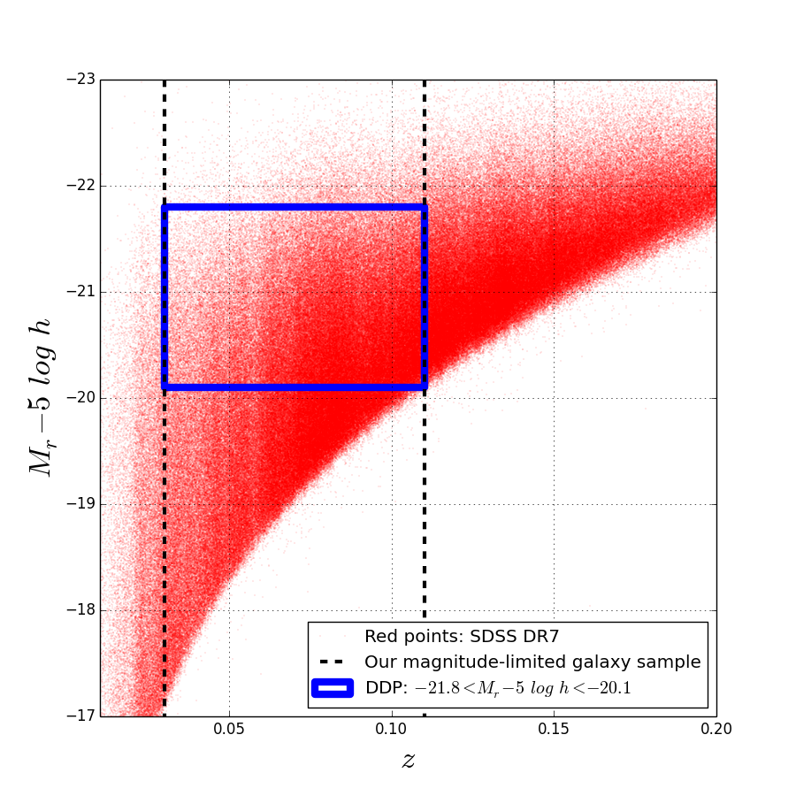
Figure 2: Absolute magnitude in the $r-$band as a function of redshift for our magnitude-limited galaxy sample. The blue solid box shows our volume-limited DDP sample. Note that our DDP sample restricts to study environments for galaxies between $0.03\leq z\leq 0.11$ as shown by the dashed lines.

2.3.2 Projected Distribution on the Sky of the Galaxy Sample

The irregular limits of the projected distribution on the sky of the SDSS-DR7 galaxies could lead to a potential bias in our overdensity measurements; they will artificially increase the frequency of low density regions and, ideally, overdensity measurements should be carried out over more continuous regions. Following Varela et al. (2012) and Cebrián & Trujillo (2014), we reduce this source of potential bias by restricting our galaxy sample to a projected area based on the following cuts:

$${\rm DEC}>\left\{\begin{array}[]{l l}0&\mbox{Southern limit}\\ -2.555556\times({\rm RA}-131^{\circ})&\mbox{Western limit}\\ -1.70909\times({\rm RA}-235^{\circ})&\mbox{Eastern limit}\\ \arcsin\left(\frac{x}{\sqrt{1-x^{2}}}\right)&\mbox{Northern limit}\end{array},\right.$$ (6)

where $x=0.93232\sin({\rm RA}-95.9^{\circ})$. This region is plotted in Figure 1 of Cebrián & Trujillo (2014).

2.3.3 Overdensity Measurements

In summary, our final magnitude-limited galaxy sample consists of galaxies in the redshift range $0.03\leq z\leq 0.11$ and galaxies within the projected area given by Equation (6), while our volume-limited DDP sample comprises galaxies with absolute magnitude satisfying $-21.8<M_{r}-5\log h<-20.1$. Based on the above specifications, we are now in a position to determine the local overdensity of each SDSS DR7 galaxy in our magnitude-limited galaxy sample.

Overdensities are estimated by counting the number of DDP galaxy neighbors, $N_{n}$, around our magnitude-limited galaxy sample in spheres of $r_{8}=8h^{-1}$ Mpc radius. While there exists various methods to measure galaxy environments, Muldrew et al. (2012) showed that aperture-based methods are more robust in identifying the dependence of halo mass on environment, in contrast to nearest-neighbors-based methods that are largely independent of halo mass. In addition, aperture-based methods are easier to interpret. For these reasons, the aperture-based method is ideal to probe galaxy environments when testing the assumptions behind the SHAM approach.

The local density is simply defined as

$$\rho_{8}=\frac{N_{n}}{4/3\pi r_{8}^{3}}.$$ (7)

We then compare the above number to the expected number density of DDP galaxies by using the global $r$-band luminosity function determined above in Section 2.2; $\bar{\rho}=6.094\times 10^{-3}h^{3}$ Mpc^-3. Finally, the local density contrast for each galaxy is determined as

$$\delta_{8}=\frac{\rho_{8}-\bar{\rho}}{\bar{\rho}}.$$ (8)

The effect of changing the aperture radius has been discussed in Croton et al. (2005). While the authors noted that using smaller spheres tends to sample underdense regions differently, they found that their conclusions remain robust due to the change of apertures. Nevertheless, smaller-scale spheres are more susceptible to be affected by redshift space distortions. Following Croton et al. (2005), we opt to use spheres of $r_{8}=8h^{-1}$ Mpc radius as the best probe of both underdense and overdense regions. Finally, note that our main goal is to understand whether halo $V_{\rm max}$ fully determines galaxy properties as predicted by SHAM, not to study the physical causes for the observed galaxy distribution with environment. Therefore, as long as we treat our mock galaxy sample, to be described in Section 3, in the same way that we treat observations, understanding the impact of changing apertures in the observed galaxy distribution is beyond the scope of this paper.

2.3.4 Measurements of the Observed $ugriz$ GLFs and the GSMF as a Function of Environmental Density

Once the local density contrast for each galaxy in the SDSS DR7 is determined, we estimate the dependence of the $ugriz$ GLFs and the GSMF with environmental density.

As in Section 2.2, we use the standard 1/$\mathcal{V}_{\rm max}$ weighting procedure. Unfortunately, the 1/$\mathcal{V}_{\rm max}$ method does not provide the effective volume covered by the overdensity bin in which the GLFs and the GSMF have been estimated and, therefore, one needs to slightly modify the 1/$\mathcal{V}_{\rm max}$ estimator. In this subsection, we describe how we estimate the effective volume.

We determine the fraction of effective volume by counting the number of DDP galaxy neighbours in a catalog of random points with the same solid angle and redshift distribution as our final magnitude-limited sample. Observe that we utilize the real position of the DDP galaxy sample defined above. We again utilized spheres of $r_{8}=8h^{-1}$ Mpc radius and create a random catalog consisting of $N_{r}\sim 2\times 10^{6}$ of points. The local density contrast for each random point is determined as in Equation (8):

$$\delta_{r_{8}}=\frac{\rho_{r_{8}}-\bar{\rho}}{\bar{\rho}},$$ (9)

where $\rho_{r_{8}}$ is the local density around random points. We estimate the fraction of effective volume by a given overdensity bin as

$$f(\delta_{8})=\frac{1}{N_{r}}\sum_{i=1}^{N_{r}}\Theta(\delta_{{r_{8}},i}).$$ (10)

Here, $\Theta$ is a function that selects random points in the overdensity range $\delta_{r_{8}}\pm\Delta\delta_{r_{8}}/2$, that is:

$$\Theta(\delta_{{r_{8}},i})=\left\{\begin{array}[]{c c}1&\mbox{if }\delta_{{r_{8}},i}\in[\delta_{r_{8}}-\Delta\delta_{r_{8}}/2,\delta_{r_{8}}+\Delta\delta_{r_{8}}/2)\\ 0&\mbox{otherwise }\end{array}.\right.$$ (11)

Table 2 lists the fraction of effective volume for the range of overdensities considered in this paper and calculated as described above. We estimate errors by computing the standard deviation of the fraction of effective volume in sixteen redshift bins equally spaced. We note that the number of sampled points gives errors that are less than $\sim 3\%$ and for most of the bins less than $\sim 1\%$, see last column of Table 2. Therefore, we ignore any potential source of error from our determination of the fraction of effective volume into the $ugriz$ GLFs and the GSMFs.

Finally, we modify the 1/$\mathcal{V}_{\rm max}$ weighting estimator to account for the effective volume by the overdensity bin as

$$\phi_{X}(M_{X}|\delta_{8})=\sum_{i=1}^{N}\frac{\omega_{i}(M_{X}\pm\Delta M_{X}/2|\delta_{r_{8}}\pm\Delta\delta_{r_{8}}/2)}{f(\delta_{8})\times\Delta M_{X}\times\mbox{$\mathcal{V}_{{\rm max},i}$}},$$ (12)

again, $M_{X}$ refers to $M_{u}$, $M_{g}$, $M_{r}$, $M_{i}$, $M_{z}$ and $\log\mbox{$M_{*}$}$. Here $\omega_{i}$ refers to the correction weight completeness factor for galaxies within the interval $M_{X}\pm\Delta M_{X}/2$ given that their overdensity is in the range $\delta_{r_{8}}\pm\Delta\delta_{r_{8}}/2$.

Table 2: Fraction of effective volume covered by the overdensity bins considered for our analysis in the SDSS DR7. Also shown is the fractional error due to the number of random points sampled.

$\delta_{{\rm min},8}$	$\delta_{{\rm max},8}$	$f(\delta_{8})\pm\delta f(\delta_{8})$	$100\%\times\delta f(\delta_{8})/f(\delta_{8})$
-1	-0.75	$0.1963\pm 0.0014$	0.713
-0.75	-0.55	$0.1094\pm 0.0010$	0.914
-0.55	-0.40	$0.0974\pm 0.0009$	0.924
-0.40	0.00	$0.2156\pm 0.0014$	0.650
0.00	0.70	$0.1800\pm 0.0012$	0.667
0.70	1.60	$0.1040\pm 0.0009$	0.866
1.60	2.90	$0.0621\pm 0.0007$	1.130
2.90	4	$0.0197\pm 0.0004$	2.030
4.00	$\infty$	$0.0153\pm 0.0004$	2.614

3 The galaxy-halo connection

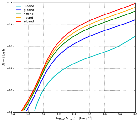
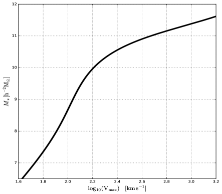
Figure 3: Left Panel: Luminosity-to-$V_{\rm max}$ relation from SHAM. The different colors indicate the band utilized for the match. Right Panel: Stellar mass-to-$V_{\rm max}$ relation. Recall that SHAM assumes that these relations are valid for centrals as well as for satellites. We report these values in Table 5.In the case of centrals $V_{\rm max}$ refers to the halo maximum circular velocity, while for satellites $V_{\rm max}$ represents the highest maximum circular velocity ($V_{\rm peak}$) reached along the subhalo’s main progenitor branch. SHAM assumes that $V_{\rm max}$ fully determines these statistical properties of the galaxies.

The main goal of this paper is to study whether one halo property, in this case $V_{\rm max}$, fully determines the observed dependence with environmental density of the $ugriz$ GLFs and the GSMF. Confirming this would significantly improve our understanding the galaxy-halo connection. In this section we describe how we constructed a mock galaxy catalog in the cosmological Bolshoi-Planck N-body simulation via (sub)halo abundance matching (SHAM).

3.1 The Bolshoi-Planck Simulation

To study the environmental dependence of the galaxy distribution predicted by SHAM, we use the N-body Bolshoi-Planck (BolshoiP) cosmological simulation (Klypin et al., 2016). This simulation is based on the $\Lambda$CDM cosmology with parameters consistent with the latest results from the Planck Collaboration. This simulation has $2048^{3}$ particles of mass $1.9\times 10^{8}\mbox{M${}_{\odot}$}h^{-1}$, in a box of side length $L_{\rm BP}=$ 250 $h^{-1}$Mpc. Halos/subhalos and their merger trees were calculated with the phase-space temporal halo finder Rockstar (Behroozi, Wechsler & Wu, 2013) and the software Consistent Trees (Behroozi et al., 2013). Entire Rockstar and Consistent Trees outputs are downloadable. Halo masses were defined using spherical overdensities according to the redshift-dependent virial overdensity $\Delta_{\rm vir}(z)$ given by the spherical collapse model, with $\Delta_{\rm vir}(z)=333$ at $z=0$. The Bolshoi-Planck simulation is complete down to halos of maximum circular velocity $\mbox{$V_{\rm max}$}\lower 2.15277pt\hbox{$\;\buildrel>\over{\sim}\;$}55$ km s^-1. For more details see Rodríguez-Puebla et al. (2016a). Next we describe our mock galaxy catalogs generated via SHAM.

3.2 Determining the Galaxy-Halo Connection

As we have explained, SHAM is a simple approach relating a halo property, such as mass or maximum circular velocity, to that of a galaxy property, such as luminosity or stellar mass. In abundance matching between a halo property and a galaxy property, the number density distribution of the halo property is matched to the number density distribution of the galaxy property to obtain the relation. Recall that SHAM assumes that that there is a one-to-one monotonic relationship between galaxies and halos, and that centrals and satellite galaxies have identical relationships (except that satellite galaxy evolution is stopped when the host halo reaches its peak maximum circular velocity). In this paper we choose to relate galaxy properties, $\mathcal{P}_{\rm gal}$, to halo maximum circular velocities $V_{\rm max}$ as

$$\int_{\mathcal{P}_{\rm gal}}^{\infty}\mbox{$\phi_{\rm gal}$}(\mathcal{P}_{\rm gal}^{\prime})d\log\mathcal{P}_{\rm gal}^{\prime}=\int_{V_{\rm max}}^{\infty}\phi_{V}(V_{\rm max}^{\prime})d\log V_{\rm max}^{\prime},$$ (13)

where $\mbox{$\phi_{\rm gal}$}(\mathcal{P}_{\rm gal})$ denotes the $ugriz$ GLF as well as the GSMF  and $\phi_{V}(\mbox{$V_{\rm max}$})$ represents the subhalo+halo velocity function, both in units of $h^{3}$ Mpc^-3 dex^-1. To construct a mock galaxy catalog of luminosities and stellar masses from the BolshoiP simulation, we apply the above procedure by using as input the global $ugriz$ GLFs and the GSMF derived in Section 2.2.

Equation (13) is the simplest form that SHAM could take as it ignores the existence of a physical scatter around the relationship between $\mathcal{P}_{\rm gal}$ and $V_{\rm max}$. Including physical scatter in Equation (13) is no longer considered valid and should be modified accordingly (for more details see Behroozi, Conroy & Wechsler, 2010). Constraints based on weak-lensing analysis (Leauthaud et al., 2012); satellite kinematics (More et al., 2009, 2011); and galaxy clustering (Zheng, Coil & Zehavi, 2007; Zehavi et al., 2011; Yang et al., 2012) have shown that this is of the order of $\sim 0.15$ dex in the case of the stellar but similar in $r-$band magnitude. There are no constraints as for the dispersion around shorter wavelengths. In addition, it is not clear how to sample galaxy properties in a system with $n$ number of properties from the joint probability distribution ${\rm prop}(\mathcal{P}_{{\rm gal},1},...,\mathcal{P}_{{\rm gal},n}|V_{\rm max}).$ Instead of that, studies that aim at to constrain the galaxy-halo connection use marginalization to constrain the probability distribution function ${\rm prop}(\mathcal{P}_{{\rm gal},i}|V_{\rm max})$ for $i$th galaxy property. In this paper we are interested in the statistical correlation of the galaxy-halo connection in which case Equation (13) is a good approximation. Studying and quantifying the physical scatter around the relations is beyond the scope of this work. Also, ignoring the scatter around the galaxy-halo connection makes it easier to interpret. For those reasons we have opted to ignore the any source of scatter in our relationships.

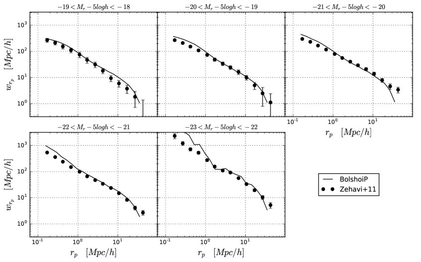
Figure 4: Two-point correlation function in five luminosity bins at $z=0.1$. The solid lines show the predicted two-point correlation based on our $r$-band magnitude-to-$V_{\rm max}$ relation from SHAM, while the circles with error bars show the same but for the SDSS DR7 (Zehavi et al., 2011).

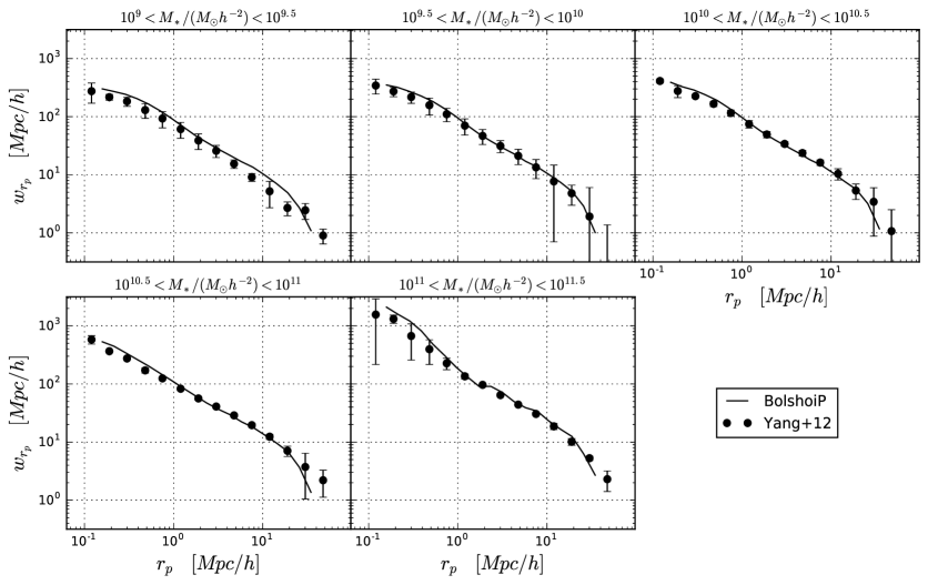
Figure 5: Two-point correlation function in five stellar mass bins. The solid lines show the predicted two-point correlation based on our stellar mass-to-$V_{\rm max}$ relation from SHAM, while the circles with error bars show the same but for SDSS DR7 (Yang et al., 2012).

Previous studies have found that for distinct dark matter halos (those that are not contained in bigger halos), the maximum circular velocity $V_{\rm max}$ is the halo property that correlates best with the hosted galaxy’s luminosity/stellar mass. This is likely because the properties of a halo’s central region, where its central galaxy resides, are better described by $V_{\rm max}$ than $M_{\rm vir}$. By comparing to observations of galaxy clustering, Reddick et al. (2013) and more recently Campbell et al. (2017) have found that for subhalos, the property that correlates best with luminosity/stellar mass is the highest maximum circular velocity reached along the main progenitor branch of the halo’s merger tree. This presumably reflects the fact that subhalos can lose mass once they approach and fall into a larger halo, while the host galaxy at the halo’s center is unaffected by this halo mass loss. Thus, in this paper we use

$$\mbox{$V_{\rm max}$}=\left\{\begin{array}[]{c l}\mbox{$V_{\rm max}$}&\mbox{Distinct halos}\\ \mbox{$V_{\rm peak}$}&\mbox{Subhalos}\end{array},\right.$$ (14)

as the halo proxy for galaxy properties $\mathcal{P}_{\rm gal}$, where $V_{\rm peak}$ is the maximum circular velocity throughout the entire history of a subhalo and $V_{\rm max}$ is at the observed time for distinct halos.

Figure 3 shows the relationships between galaxy luminosities $u$, $g$, $r$, $i$, and $z$ and galaxy stellar masses to halo maximum circular velocities. Table 5, reports the values from Figure 3. Most of these relationships are steeply increasing with $V_{\rm max}$ for velocities below $\mbox{$V_{\rm max}$}\sim 160$ km s^-1. At higher velocities the relationships are shallower. The shapes of these relations are governed mostly by the shapes of the GLFs and GSMF, since the velocity function $\phi_{V}$ is approximately a power-law over the range plotted in Figure 3, see Rodríguez-Puebla et al. (2016a).

Note that at this point every halo and subhalo in the BolshoiP simulation at rest frame $z=0$ has been assigned a magnitude in the five bands $u$, $g$, $r$, $i$, and $z$ and a stellar mass $M_{*}$. Therefore, one might be tempted to correlate galaxy colors such as red or blue (i.e. differences between galaxy magnitudes) with halo properties. If we did this, we would be ignoring the scatter around our luminosity/stellar mass-to-$V_{\rm max}$ relationships, and galaxies with the same magnitude or $M_{*}$ would have the same color, contrary to observation. Fortunately, including a scatter around those relationships will not impact our conclusions given that i) the scatter does not substantially impact the results presented in Figure 3 and ii) we are here interested only in the statistical correlation of the galaxy properties with environment. Nevertheless, in Section 4.2.1 we will study the statistical correlation between color and environment for all galaxies, and separately for central and satellite galaxies.

As a sanity check, we show that our mock galaxy catalog in the BolshoiP reproduces the projected two-point correlation function of SDSS galaxies. Figures 4 and 5 show, respectively, that this is the case for the $r$-band and stellar mass projected two point correlation functions. In the case of $r$-band, we compared to Zehavi et al. (2011) who used $r$-band magnitudes at $z=0.1$. We transformed our $r$-band magnitudes to $z=0.1$ by finding the correlation between model magnitudes at $z=0$ and at $z=0.1$ from the tables of the NYU-VAGC. For the projected two point correlation function in stellar mass bins we compare with Yang et al. (2012).

3.3 Measurements of the mock $ugriz$ GLFs and the GSMF as a function of environment

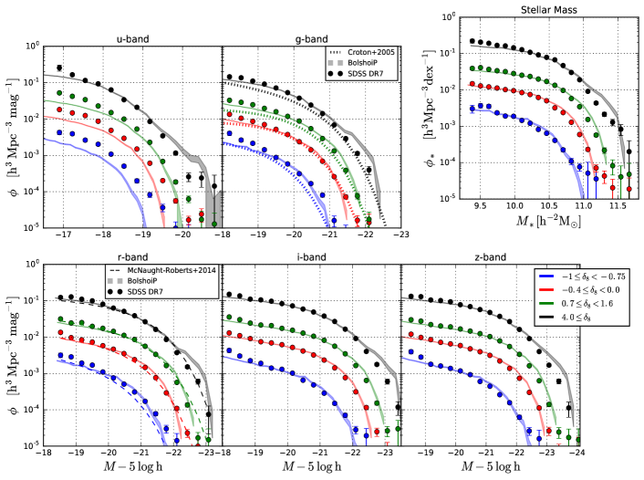
Figure 6: Comparison between the observed SDSS DR7 $ugriz$ GLFs and GSMF, filled circles with error bars, and the ones predicted based on the BolshoiP simulation from SHAM, shaded regions, at four environmental densities in spheres of radius 8 $h^{-1}$Mpc. We also reproduce the best fitting Schechter functions to the $r$-band GLFs from the GAMA survey (McNaught-Roberts et al., 2014). Observe that SHAM predictions are in excellent agreement with observations, especially for the longest wavelength bands and stellar mass.

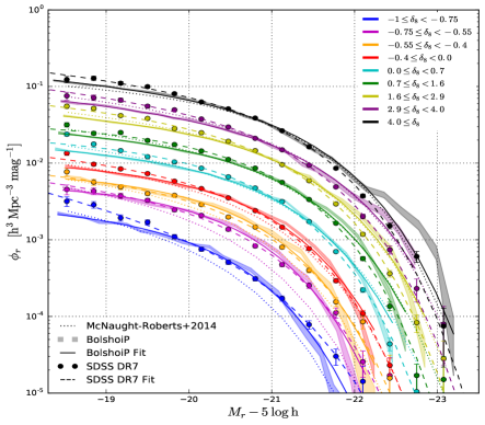
Figure 7: Left Panel: Comparison between the observed $r-$band GLF with environmental density in spheres of 8 $h^{-1}$Mpc, filled circles with error bars, and the ones predicted based on the BolshoiP simulation from SHAM, shaded regions. The dashed and solid lines show the best fitting Schechter functions to the observed and the mocked $r-$band GLFs while the dotted lines show the same but from the GAMA survey (McNaught-Roberts et al., 2014). Right Panel: Similar to the left panel but for the GSMF with environmental density. Here again the dashed and solid lines are the best fitting Schechter functions to the observed and mocked GSMFs.

Our mock galaxy catalog is a volume complete sample down to halos of maximum circular velocity $\mbox{$V_{\rm max}$}\sim 55$ km$s^{-1}$, corresponding to galaxies brighter than $M_{r}-5\log h\sim-14$, see Figure 3. This magnitude completeness is well above the completeness of the SDSS DR7. Thus, galaxies selected in the absolute magnitude range $-21.8<M_{r}-5\log h<-20.1$ define a volume-limited DDP sample. In other words, incompleteness is not a problem for our mock galaxy catalog. Overdensity and density contrast measurements for each mock galaxy in the BolshoiP simulation are obtained as described in Section 2.3.3.

We estimate the dependence of the $ugriz$ GLFs with environment in our mock galaxy catalog as

$$\phi_{X}(M_{X}|\delta_{8})=\sum_{i=1}^{N}\frac{\omega_{i}(M_{X}\pm\Delta M_{X}/2|\delta_{r_{8}}\pm\Delta\delta_{r_{8}}/2)}{\Delta M_{X}f_{\rm BP}(\delta_{8})L_{\rm BP}^{3}}.$$ (15)

Here, $\omega_{i}=1$ if a galaxy is within the interval $M_{X}\pm\Delta M_{X}/2$ given that its overdensity is in the range $\delta_{r_{8}}\pm\Delta\delta_{r_{8}}/2$, otherwise it is 0. Again, $M_{X}$ refers to $M_{u}$, $M_{g}$, $M_{r}$, $M_{i}$, $M_{z}$ and $\log\mbox{$M_{*}$}$. The function $f_{\rm BP}(\delta_{8})$ is the fraction of effective volume by a given overdensity bin for the BolshoiP simulation. In order to determine $f_{\rm BP}(\delta_{8})$, we create a random catalog of $N_{r}\sim 1.2\times 10^{6}$ points in a box of side length identical to the BolshoiP simulation, i.e., $L_{\rm BP}=$ 250 $h^{-1}$Mpc. Using Equation (10) allows us to calculate $f_{\rm BP}(\delta_{8})$.

4 Results on Environmental Density Dependence

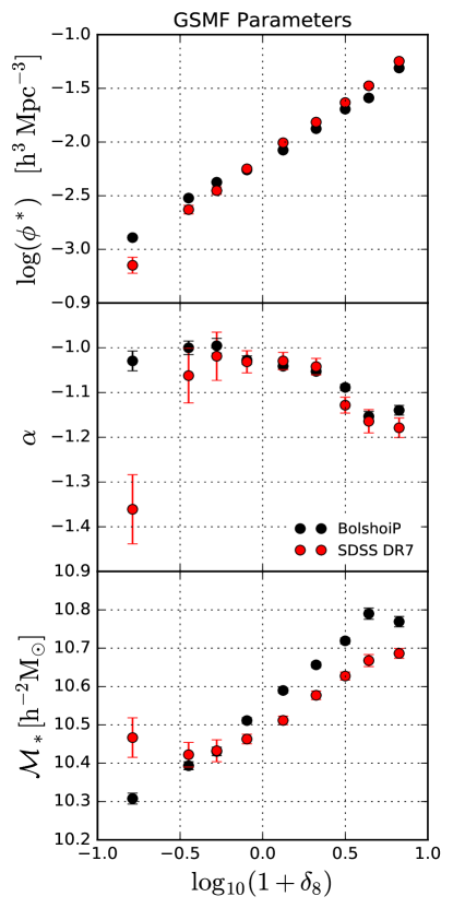
Figure 8: Left Panel: The dependence of the $r-$band Schechter function parameters on environmental overdensity $\delta_{8}$ in spheres of 8 $h^{-1}$ Mpc (Eq (8)). Right Panel: The dependence of the galaxy stellar mass function Schechter parameters on environmental density.

In this section we present our determinations for the environmental density dependence of the $ugriz$ GLFs and the GSMF from the SDSS DR7 and the BolshoiP. Here, we will investigate how well the assumption that the statistical properties of galaxies are fully determined by $V_{\rm max}$ can predict the dependence of the $ugriz$ GLFs and GSMF with environment. We will show that predictions from SHAM are in remarkable agreement with the data from the SDSS DR7, especially for the longer wavelength bands. Finally, we show that SHAM also reproduces the correct dependence on environmental density of both the $r$-band GLFs and GSMF for centrals and satellites, although it fails to reproduce the observed relationship between environment and color.

4.1 SDSS DR7

Figure 6 shows the dependence of the SDSS DR7 $ugriz$ GLFs as well as the GSMF with environmental density measured in spheres of radius 8 $h^{-1}$Mpc. For the sake of the simplicity, we present only four overdensity bins in Figure 6. In Figure 7 we show the determinations in nine density bins for the $r$-band GLFs and GSMF. In order to compare with recent observational results we use identical environment density bins as in McNaught-Roberts et al. (2014), who used galaxies from the GAMA survey to measure the dependence of the $r$-band GLF on environment over the redshift range $0.04<z<0.26$ in spheres of radius of 8 $h^{-1}$Mpc.

The $r-$band panel of Figure 6 shows that our determinations are in good agreement with results from the GAMA survey. In the $g$-band panel of the same Figure, we present a comparison with the previously published results by Croton et al. (2005), who used the 2dF Galaxy Redshift Survey to measure the dependence of the $b_{\rm J}$-band GLFs at a zero redshift rest-frame in spheres of radius of 8 $h^{-1}$Mpc. We convert the $b_{\rm J}$-band GLFs from Croton et al. (2005) to the $g$-band by applying a shift of -0.25 to their magnitudes, that is, $M_{g}=M_{b_{\rm J}}-0.25$ (Blanton et al., 2005a). We observe good agreement with the result of Croton et al. (2005) for most of our density bins. A better comparison would have used identical density bins; however, the density bins used by Croton et al. (2005) are close to ours. Finally, in Figure 6 we also extend previous results by presenting the GLFs for the $u$, $i$ and $z$ bands and for the GSMF. We are not aware of any published low redshift GLFs for the $u$, $i$ and $z$ bands.

The left panel of Figure 7 shows again the dependence of the GLF in the $r-$band, but now for all our overdensity bins, filled circles with error bars. In order to report an analytical model for the luminosity functions, we fit observations to a simple Schechter function; observations show that this model is a good description for the data, given by

$$\phi(M)=\frac{\ln 10}{2.5}\phi^{*}10^{0.4(M^{*}-M)\left(1+\alpha_{1}\right)}\exp\left(-10^{0.4\left(M^{*}-M\right)}\right),$$ (16)

in units of $h^{3}$ Mpc^-3 mag^-1. The best fit to simple Schechter functions are shown as the dashed lines in the same plot, and we report the Schechter parameters as a function of the density contrast in the left panel of Figure 8. The best fitting parameters are listed in Table 3. For comparison, we reproduce the best fit to a Schechter function from McNaught-Roberts et al. (2014), dotted lines.

Figure 8 shows that the normalization parameter of the Schechter function, $\phi^{*}$, depends strongly on density. There are almost two orders of magnitude difference between the least and the highest density bins; see also Table 3. In contrast, the faint-end slope, $\alpha$, remains practically constant with environment with a value of $\alpha=-1.0$ to $-1.2$. Note, however, that our analysis of the SDSS observations shows that the GLF becomes steeper in the least dense environment, with $\alpha\sim-1.7$. The characteristic magnitude of the Schechter function, $M^{*}$, evolves only little with environment between $-1\lower 2.15277pt\hbox{$\;\buildrel<\over{\sim}\;$}\delta_{8}\lower 2.15277pt\hbox{$\;\buildrel<\over{\sim}\;$}0$ but it increases above $\delta_{8}\sim 0$. Finally, in the same figure, we reproduce the best fitting model parameters reported in McNaught-Roberts et al. (2014). In general, our determinations are in good agreement with the trends reported in McNaught-Roberts et al. (2014) even at faint magnitudes, as is shown in Figures 7 and 8. This is reassuring since the GAMA survey is deeper than the SDSS which could result in a much better determination of the faint-end. In addition, the subtended area by the GAMA survey is much smaller than that of the SDSS, which could have resulted in GAMA underestimating the abundance of massive galaxies in low-density environments. The reason for this is because the limited volume of GAMA does not adequately sample these rather rare galaxies in low-density regions.

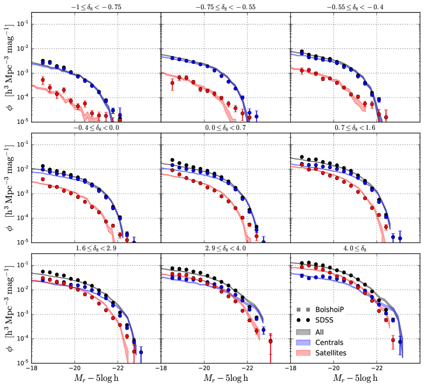
Figure 9: The dependence on $r$-band magnitude of the GLFs in nine bins of environmental density in $8h^{-1}$ Mpc spheres for all galaxies, central galaxies, and satellite galaxies. Filled circles with error bars show the results from the SDS DR7 while shaded areas show the SHAM predictions from the BolshoiP simulation. There is a remarkable agreement between observations and SHAM predictions, even when dividing between centrals and satellites.

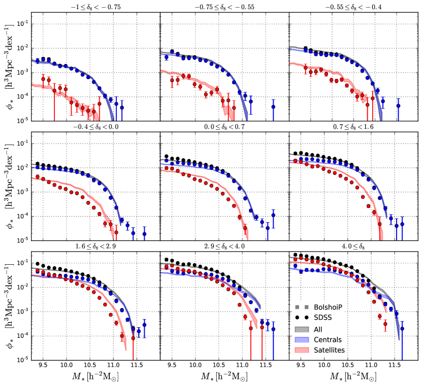
Figure 10: Similarly to Figure 9 but for the GSMF for all galaxies, central galaxies, and satellite galaxies. Filled circles with error bars show the results from the SDS DR7 while shaded areas show the SHAM predictions from the BolshoiP simulation. While there is good agreement between observations and SHAM predictions for all galaxies and centrals, there is some tension with the SHAM predictions of the satellite GSMF.

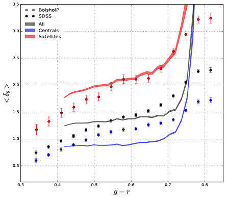
Figure 11: Mean density in $8h^{-1}$ Mpc spheres as a function of galaxy $g-r$ color, from the SDSS DR7 (shaded regions, representing the standard deviation) and the mean density predicted by SHAM based on the BolshoiP simulation, filled circles with error bars. We present the mean density for all, central, and satellite galaxies as indicated by the labels. SHAM fails to predict the correct relationship between mean density and galaxy colors for all galaxies and central galaxies. In contrast, the SHAM prediction for satellite galaxies is in better agreement with observations.

The right panel of Figure 7 shows the dependence of the GSMF for all our overdensity bins as well as their corresponding best fit to simple Schechter functions, filled circles with error bars and solid lines, respectively. In this case the Schechter function is given by

$$\phi_{*}(\mbox{$M_{*}$})=\phi_{1}^{*}\times{\ln 10}\times\left(\frac{\mbox{$M_{*}$}}{\mathcal{M}_{1}^{*}}\right)^{1+\alpha_{1}}\exp\left(-\frac{\mbox{$M_{*}$}}{\mathcal{M}_{1}^{*}}\right),$$ (17)

with units of $h^{3}$ Mpc^-3 dex^-1. We report the best fitting parameters in Table 4. The right panel of Figure 8 presents the Schechter parameters for the GSMFs as a function of the density contrast. Similarly to the GLFs, the normalization parameter for the GSMF, $\phi^{*}$, depends strongly on density as a power-law and there are approximately two orders of magnitude difference between the GLFs in the least and the most dense environments. As for the faint-end slope, $\alpha$, we observe that the general trend is that in high density environments the GSMF becomes steeper than in low density environments. Nonetheless, we observe, again, that in the lowest density bin the GSMF becomes steeper than other density bins. The characteristic stellar mass of the Schechter function, $\mathcal{M}_{*}$ increases with the environment at least for densities greater than $\delta_{8}\sim 0$. In contrast, below $\delta_{8}\sim 0$ it remains approximately constant.

Table 3: Best fitting parameters from the observed SDSS DR7 GLFs

Galaxy Luminosity Functions
SDSS DR7
$\delta_{{\rm min},8}$	$\delta_{{\rm max},8}$	$\alpha$	$M^{*}-5\log h$	$\log\phi^{*}$ $\left[h^{3}{\rm Mpc}^{-3}{\rm mag}^{-1}\right]$
-1	-0.75	$-1.671\pm 0.092$	$-20.650\pm 0.131$	$-2.938\pm 0.095$
-0.75	-0.55	$-1.265\pm 0.077$	$-20.456\pm 0.086$	$-2.391\pm 0.051$
-0.55	-0.40	$-1.178\pm 0.068$	$-20.490\pm 0.073$	$-2.224\pm 0.041$
-0.40	0.00	$-1.217\pm 0.032$	$-20.568\pm 0.033$	$-2.031\pm 0.019$
0.00	0.70	$-1.120\pm 0.025$	$-20.604\pm 0.026$	$-1.754\pm 0.013$
0.70	1.60	$-1.092\pm 0.023$	$-20.703\pm 0.025$	$-1.556\pm 0.012$
1.60	2.90	$-1.230\pm 0.033$	$-20.870\pm 0.016$	$-1.408\pm 0.015$
2.90	4	$-1.292\pm 0.028$	$-20.981\pm 0.040$	$-1.280\pm 0.023$
4.00	$\infty$	$-1.275\pm 0.005$	$-21.000\pm 0.034$	$-1.045\pm 0.020$
BolshoiP+SHAM
-1	-0.75	$-1.0963\pm 0.0264$	$-20.1018\pm 0.0319$	$-2.6084\pm 0.0172$
-0.75	-0.55	$-1.0214\pm 0.0206$	$-20.2498\pm 0.0238$	$-2.2478\pm 0.0127$
-0.55	-0.40	$-1.0462\pm 0.0225$	$-20.3727\pm 0.0273$	$-2.1260\pm 0.0147$
-0.40	0.00	$-1.0828\pm 0.0129$	$-20.5454\pm 0.0193$	$-2.0225\pm 0.0096$
0.00	0.70	$-1.1274\pm 0.0087$	$-20.7486\pm 0.0142$	$-1.8634\pm 0.0075$
0.70	1.60	$-1.1453\pm 0.0086$	$-20.8882\pm 0.0204$	$-1.6760\pm 0.0079$
1.60	2.90	$-1.1790\pm 0.0092$	$-21.0189\pm 0.0220$	$-1.4913\pm 0.0090$
2.90	4	$-1.2451\pm 0.0154$	$-21.1841\pm 0.0354$	$-1.3821\pm 0.0179$
4.00	$\infty$	$-1.2227\pm 0.0129$	$-21.1285\pm 0.0300$	$-1.0924\pm 0.0149$

Table 4: Best fitting parameters from the observed SDSS DR7 GSMF

Galaxy Stellar Mass Functions
SDSS DR7
$\delta_{{\rm min},8}$	$\delta_{{\rm max},8}$	$\alpha$	$\mathcal{M}_{*}$ $\left[h^{-2}\mbox{M${}_{\odot}$}\right]$	$\log\phi^{*}$ $\left[h^{3}{\rm Mpc}^{-3}{\rm dex}^{-1}\right]$
-1	-0.75	$-1.361\pm 0.077$	$10.467\pm 0.052$	$-3.148\pm 0.075$
-0.75	-0.55	$-1.062\pm 0.061$	$10.422\pm 0.032$	$-2.630\pm 0.040$
-0.55	-0.40	$-1.019\pm 0.054$	$10.433\pm 0.029$	$-2.453\pm 0.035$
-0.40	0.00	$-1.031\pm 0.025$	$10.463\pm 0.012$	$-2.250\pm 0.015$
0.00	0.70	$-1.029\pm 0.019$	$10.511\pm 0.011$	$-2.006\pm 0.012$
0.70	1.60	$-1.042\pm 0.018$	$10.577\pm 0.011$	$-1.815\pm 0.012$
1.60	2.90	$-1.128\pm 0.018$	$10.627\pm 0.011$	$-1.632\pm 0.013$
2.90	4	$-1.164\pm 0.026$	$10.668\pm 0.016$	$-1.477\pm 0.021$
4.00	$\infty$	$-1.179\pm 0.022$	$10.686\pm 0.013$	$-1.248\pm 0.017$
BolshoiP+SHAM
-1	-0.75	$-1.0293\pm 0.0222$	$10.3077\pm 0.0142$	$-2.8903\pm 0.0176$
-0.75	-0.55	$-1.0000\pm 0.0151$	$10.3933\pm 0.0105$	$-2.5222\pm 0.0128$
-0.55	-0.40	$-0.9954\pm 0.0162$	$10.4306\pm 0.0110$	$-2.3743\pm 0.0138$
-0.40	0.00	$-1.0275\pm 0.0094$	$10.5112\pm 0.0074$	$-2.2602\pm 0.0088$
0.00	0.70	$-1.0411\pm 0.0074$	$10.5896\pm 0.0065$	$-2.0754\pm 0.0073$
0.70	1.60	$-1.0528\pm 0.0073$	$10.6564\pm 0.0069$	$-1.8757\pm 0.0075$
1.60	2.90	$-1.0885\pm 0.0069$	$10.7191\pm 0.0075$	$-1.6939\pm 0.0081$
2.90	4	$-1.1533\pm 0.0112$	$10.7898\pm 0.0146$	$-1.5891\pm 0.0154$
4.00	$\infty$	$-1.1396\pm 0.0109$	$10.7691\pm 0.0135$	$-1.3106\pm 0.0143$

4.2 Comparison to Theoretical Determinations: SHAM

Figure 6 compares our observed $ugriz$ GLFs and the results derived from the mock galaxy sample based on SHAM. In general, we observe a remarkable agreement between observations and SHAM. This statement is true for all the luminosity bands as well as for stellar mass and for most of the density bins. This remarkable agreement is not a trivial result since we are assuming that $V_{\rm max}$ fully determines the magnitudes in the $u$, $g$, $r$, $i$, and $z$ bands and stellar mass $M_{*}$ in every halo in the simulation. Additionally, in Section 3 we noted that the shape of the galaxy-halo connection is governed, mainly, by the global shape of the galaxy number densities. Moreover, while we have defined our volume-limited DDP sample as for the SDSS observations, it is subject to the assumptions behind SHAM as well. In addition, the real correlation between $r$-band magnitude and all other galaxy properties is no doubt more complex than just monotonic relationships without scatters, as is derived in SHAM.

Note, however, that there are some discrepancies towards bluer bands and low densities. Shorter wavelengths are more affected by recent star formation, and more likely to be related to halo mass accretion rates (Rodríguez-Puebla et al., 2016b, and references therein), while infrared magnitudes depend more strongly on stellar mass. This perhaps just reflects that stellar mass is the galaxy property that most naturally correlates with $V_{\rm max}$. Indeed, when comparing the environmental dependence of the observed and the mock GSMF we observe, in general, rather good agreement.

The left panel of Figure 7 compares the resulting dependence of the observed $r$-band GLFs with environment and the predictions based on SHAM for all our overdensity bins. This again shows the remarkable agreement between observations and SHAM for all our density bins. Similarly, the right panel of Figure 7 compares the observed GSMF with our predictions based on SHAM. Left panel of Figure 8 compares the best fitting Schechter parameters for the $r$-band magnitude while the right panel shows the same but for stellar masses. In order to make a meaningful comparison with observations, we fit the observed GLFs and GSMF of the SDSS DR7 over the same dynamical ranges. In general, we observe a good agreement between predictions from SHAM and the results from the SDSS DR7.

While Figure 7 shows that the general trends are well predicted by SHAM, there are some differences that are worth discussing. SHAM is able to recover the overall normalization of the $r$-band GLF and the GSMF, but it slightly underpredicts the number of faint galaxies and it also underpredicts the high-mass end in low-density environments. In high-density environments SHAM overpredicts the number of galaxies at the high mass end. A natural explanation for these differences could be the dependence of the galaxy-halo connection with environment. Recall that we are assuming zero scatter in the galaxy-halo connection. Despite the differences noted above, the extreme simplicity of SHAM captures extremely well the dependences with environmental density of the galaxy distribution. This is remarkable and, as we noted earlier, it might not be expected since halo properties depend on the local environment as well as the large-scale environment. In order to understand better the success of SHAM and the nature of the above discrepancies, we now turn our attention to the dependence with environment of the $r$-band GLFs and GSMF of central and satellite galaxies separately.

4.2.1 SHAM Predictions for the Central and Satellite GLF and GSMF

Figures 9 and 10 show respectively the dependence on environmental density of the $r$-band GLFs and GSMF for all galaxies, and separately for centrals and satellites. The circles with error bars show the results when using the memberships from the SDSS DR7 Yang et al. (2012) galaxy group catalog, while the shaded areas show the predictions from SHAM based on the BolshoiP simulation. When dividing the population between centrals and satellites, in general SHAM captures the observed dependences from the SDSS DR7 Yang et al. (2012) galaxy group catalog. This simply reflects that the fraction of subhalos increases as a function of the environment as well as the chances of finding high mass (sub)halos in dense environments.

The agreement is particularly good for centrals. However, the satellite $r$-band GLF is in much better agreement with observations than the satellite GSMF: for the $r$-band GLF we observe a marginal difference only, while SHAM predicts that there are more galaxies around the knee of the GSMF compared to what is observed. It is not clear why we should expect this difference, but a potential explanation could be that satellite galaxies are much more sensitive to their local environment and to the definition of the DDP population. To help build intuition, recall that SHAM assigns every halo in the simulation five magnitudes in the $u$, $g$, $r$, $i$, and $z$ bands and stellar mass $M_{*}$. Consider now that the relationship between $r$-band magnitude and all other galaxy properties are just monotonic and with zero scatter, as explained earlier. Thus, this oversimplification of much more complex relationships is affecting the measurements of environmental dependences in satellite galaxies especially when these are projected in other observables. Possibly, when using a stellar mass-based DDP population the problem will be inverted. In other words, we might observe a marginal difference between SHAM and the GSMFs but a larger differences between SHAM and the GLFs. Of course central galaxies are not exempt from also being affected, but given the good agreement with observations we conclude that the effect is only marginal. Another possible explanation is that the assumption of identical relations between centrals and satellites is more valid for the $r$-band luminosity than for the stellar mass. That is, the stellar mass of satellite galaxies perhaps varies more strongly with $V_{\rm max}$ than the $r$-band luminosity does.

A third possible explanation is that group finding algorithms are subject to errors. In a recent paper, Campbell et al. (2015) showed that there are two main sources of errors that could affect the comparison in Figures 9 and 10: i) central/satellite designation and ii) group membership determination. In that paper, the authors showed that the Yang et al. (2007) group finder algorithm tends to misidentify central galaxies systematically with increasing group mass. In other words, satellites are sometimes mistakenly identified as centrals. Consequently, the GLFs and the GSMF for centrals and satellites will be affected towards the bright-end. Note, however, that Campbell et al. (2015) showed that for each satellite that is misidentified as a central, approximately a central is misidentified as a satellite in the Yang et al. (2007) group finder. Thus, in the Yang et al. (2007) group finder central/satellite designation is the main source of error rather than the group membership determination. While this a source of error that should be taken into account in our analysis, it is likely that this is not the main source of difference between observations and SHAM predictions. The reason is that there exists the above compensation effect in the identification of centrals and satellite galaxies which could leave, perhaps, the GLFs and the GSMF of centrals and satellites with little or no changes.

Finally, as we noted earlier, Figure 7 shows that SHAM overpredicts the number of high mass galaxies in high mass bins. Figures 9 and 10 show that this excess of galaxies is due to central galaxies. We will discuss this in the light of the dependence of the galaxy-halo connection with environment in Section 5.

4.2.2 The Relationship Between Color and Mean Environmental Density

Figure 11 shows the mean density as a function of the $g-r$ color separately for all galaxies, centrals, and satellites. The filled circles with error bars show the mean density measured from the Yang et al. (2012) galaxy group catalog while the shaded areas show the same but for the BolshoiP simulation. SHAM is unable to predict the correct correlation between mean density and galaxy colors for all and central galaxies. SHAM predicts that, statistically speaking, the large-scale mean environmental density varies little with the colors of central galaxies, except that the reddest galaxies on average lie in the densest environments. Actually, this is not surprising since we assumed that the $ugriz$ bands and stellar mass are independent of environment when constructing our mock galaxy catalog and the above is simply showing that one halo property does not fully determine the statistical properties of the galaxies. Other halo properties that vary with environment should instead be used in order to reproduce the correct trends with environment. Extensions to SHAM in which halo age is matched to galaxy age/color at a fixed luminosity/stellar mass and halo mass (see e.g., Hearin & Watson, 2013; Masaki, Lin & Yoshida, 2013) are promising approaches that could help to better explain the trends with observations. Nonetheless, SHAM predictions are in better agreement with the observed correlation of density with color for satellite galaxies.

5 Summary and Discussion

Subhalo abundance matching (SHAM) makes the assumption that one (sub)halo property fully determines the statistical properties of their host galaxies. Therefore, SHAM implies that i) the galaxy-halo connection is identical between halos and subhalos, and ii) the dependence of galaxy properties on environmental density comes entirely from the corresponding dependence on density of this (sub)halo property. The halo property that this paper explores for SHAM is the quantity $V_{\rm max}$, which is defined in Equation (14) as the maximum circular velocity for distinct halos, while for subhalos it the peak maximum circular velocity $V_{\rm peak}$ reached along the halo’s main progenitor branch. This is the most robust halo and subhalo property for SHAM (see, e.g., Reddick et al., 2013; Campbell et al., 2017). The galaxy properties we studied are the $ugriz$ GLFs as well as the GSMF, which we determined from the SDSS DR7. We compared these observations with SHAM predictions from a mock galaxy catalog based on the BolshoiP simulation (Klypin et al., 2016; Rodríguez-Puebla et al., 2016a). SHAM assigns every halo in the BolshoiP simulation magnitudes in the five SDSS bands $u$, $g$, $r$, $i$ and $z$ and also a stellar mass $M_{*}$(Figure 3 and Appendix). We tested the assumptions behind SHAM by comparing the predicted and observed dependence of the $ugriz$ GLFs as well as the GSMF on the environmental density from the SDSS DR7 Yang et al. (2012) galaxy group catalog. The main results and conclusions are as follows:

• In general, the environmental dependence of the $ugriz$ GLFs predicted by SHAM are in good agreement with the observed dependence from the SDSS DR7. This is especially true for $r$ and infrared bands. Theoretically the stellar mass is the galaxy property that is expected to depend more strongly on halo $V_{\rm max}$, while bluer bands also reflect recent effects of star formation.

• We show that the environmental dependence of the GSMF predicted by SHAM is in remarkable agreement with the observed dependence from the SDSS DR7, reinforcing the above conclusion.

• When dividing the galaxy population into centrals and satellites SHAM predicts the correct dependence of the observed $r$-band GLF and GSMF for centrals and satellite galaxies from the Yang et al. (2012) group galaxy catalog.

• While SHAM predicts GLFs and the GSMF that are in remarkable agreement with observations even when the galaxy population is separated between centrals and satellites, SHAM does not predict the observed average relation between $g-r$ color and mean environmental density. This is especially true for central galaxies, while the correlation obtained for satellite galaxies is in better agreement with observations.

Many previous authors have studied the correlation between galaxies and dark matter halos with environment both theoretically and observationally (see, e.g., Avila-Reese et al., 2005; Baldry et al., 2006; Blanton & Berlind, 2007; Maulbetsch et al., 2007; Tinker, Wetzel & Conroy, 2011; Lacerna et al., 2014; Lee et al., 2017; Yang et al., 2017, and many more references cited therein). While most of these authors have focused on understanding this correlation by studying the galaxy distribution as a function of color, star formation or age and environment at a fixed $M_{*}$, here we take a different approach and exploit the extreme simplicity of SHAM. Firstly, there are no special galaxies in SHAM. Second, SHAM can be applied to any galaxy property distribution. Thus, in our framework a halo and a subhalo with identical $V_{\rm max}$ will host galaxies with identical luminosities and stellar mass, no matter the halo’s environmental density or position in the cosmic web. Our results are consistent with previous findings that halo $V_{\rm max}$ could be enough to determine the luminosities and stellar masses. However, we have also shown that SHAM is unable to reproduce the correct correlation between galaxy color and the mean density $\delta_{8}$ on a scale of 8 $h^{-1}$ Mpc. This result implies that additional halo properties that depend in some way on the halo environment (e.g., Lee et al., 2017) should be employed to correctly reproduce the relationship between $\delta_{8}$ and galaxy color.

Does the above imply that the galaxy-halo connection should depend on environment? On the one hand, from observations we have learned that the statistical properties of the galaxies such as color and star formation change with environment in the direction that low density environments are mostly populated by blue/star-forming galaxies while dense environments are mostly populated with red/quenched galaxies (see for e.g., Hogg et al., 2003; Baldry et al., 2006; Tomczak et al., 2017). On the other hand, the shape of the luminosity-to-$V_{\rm max}$ and the stellar mass-to-$V_{\rm max}$ relations, Figure 3, contain information about the process that regulated the star formation in galaxies. Therefore, it is not a bad idea to consider that the differences described in Figure 7 are the result that the galaxy-halo connection could change with environment. For the sake of the simplicity, consider the GSMF of central galaxies derived in the case of zero scatter around the $\mbox{$M_{*}$}=\mbox{$M_{*}$}(\mbox{$V_{\rm max}$})$ relationship. Therefore, Equation (13) can be rewritten to give the GSMF as

$$\phi_{*}(\mbox{$M_{*}$})=\phi_{V}(\mbox{$V_{\rm max}$}(\mbox{$M_{*}$}))\times\alpha_{\rm gal},$$ (18)

while the dependence with environment of the GSMF of central galaxies is given by

$$\phi_{*}(\mbox{$M_{*}$}|\delta_{8})=\phi_{V}(\mbox{$V_{\rm max}$}(\mbox{$M_{*}$})|\delta_{8})\times\alpha_{\rm gal},$$ (19)

where $\alpha_{\rm gal}\equiv d\log\mbox{$V_{\rm max}$}(\mbox{$M_{*}$})/d\log\mbox{$M_{*}$}$ is the logarithmic slope of the $\mbox{$M_{*}$}=\mbox{$M_{*}$}(\mbox{$V_{\rm max}$})$ relationship assumed to be independent of environment. Next, consider the simplest case in which $\phi_{V}(\mbox{$V_{\rm max}$}|\delta_{8})$ is a double power law such that $\phi_{V}(\mbox{$V_{\rm max}$}|\delta_{8})\propto V_{\rm max}^{\beta(\delta_{8})}$ for $V_{\rm max}\ll V_{\rm max}^{*}(\delta_{8})$ and $\phi_{V}(\mbox{$V_{\rm max}$}|\delta_{8})\propto V_{\rm max}^{\gamma(\delta_{8})}$ for $V_{\rm max}\gg V_{\rm max}^{*}(\delta_{8})$ where $V_{\rm max}^{*}(\delta_{8})$ is a characteristic velocity and we have emphasized that the parameters $\beta,\gamma$ and $V_{\rm max}^{*}$ depend on the environment. In order to simplify even further the problem, consider that the $\mbox{$M_{*}$}=\mbox{$M_{*}$}(\mbox{$V_{\rm max}$})$ relationship is a power law relation at low masses with logarithmic slope $\alpha_{\rm gal,low}$ while at high masses it is also a power law with logarithmic slope of $\alpha_{\rm gal,high}$ . Based on the above, we can write the dependence with environment of the GSMF of central galaxies in the limit cases

$$\phi_{*}(\mbox{$M_{*}$}|\delta_{8})\propto\left\{\begin{array}[]{@{}l@{}l@{}}\alpha_{\rm gal,low}\times M_{*}^{\beta(\delta_{8})/\alpha_{\rm gal,low}}&\mbox{if }V_{\rm max}\ll V_{\rm max}^{*}(\delta_{8})\\ \alpha_{\rm gal,high}\times M_{*}^{\gamma(\delta_{8})/\alpha_{\rm gal,high}}&\mbox{if }V_{\rm max}\gg V_{\rm max}^{*}(\delta_{8})\end{array}.\right.$$ (20)

Thus, if $\alpha_{\rm gal,low}$ and $\alpha_{\rm gal,high}$ are independent of environment the resulting shape and dependence of $\phi_{*}(\mbox{$M_{*}$}|\delta_{8})$ with environment can be simply understood as the dependence with environment of the slopes $\beta$ and $\gamma$ of the halo velocity function.

By looking to the least (voids-like) and highest (cluster-like) density environments from Figure 10, upper left and bottom right panels respectively, we can use the above model in order to understand how the galaxy-halo connection may depend on environment. The voids-like GSMF from Figure 10 shows that SHAM tends to underpredict the number density of central galaxies both at the low and high mass ends. In other words, the slopes predicted by SHAM at the low and high mass ends are, respectively, too shallow and steep compared to observations. Inverting this would require, based on Equation (20), to make the slopes $\alpha_{\rm gal,low}$ and $\alpha_{\rm gal,high}$ shallower and steeper, respectively, to what we derived from SHAM, see the right panel of Figure 3. This implies that in low density environments at a fixed $V_{\rm max}$ halos had been more efficient in forming stars both for at the low and high mass end. In contrast, the high density GSMF from Figure 10 shows that SHAM tends to overpredict the number density of central galaxies at the high mass end. In this case, we invert the above trend by making the high mass end slope $\alpha_{\rm gal,high}$ more shallow compared to what is currently derived from SHAM. This implies that the star formation efficiency has been suppressed in high mass halos residing in high density environments with respect to the predictions of SHAM.

The above limiting cases show that the galaxy-halo connection is expected to change with environment in the direction that halos in low density environment should be more efficient in transforming their gas into stars while in high density environments halos have become more passive. This is indeed consistent with the color/star formation trends that have been observed in large galaxy surveys. Of course, our discussion is an oversimplification, and in order to model exactly how the galaxy-halo connection depends on environment we would need to use the dependence of the GSMF with environment as an extra observational constraint for the galaxy-halo connection. In a recent series of papers Tinker et al. (2017c, b) and Tinker et al. (2017a) studied the galaxy-halo connection in the light of the relation between the star formation and environment at a fixed stellar and halo mass, obtaining similar conclusions to ours. That is, above-average galaxies with above average star formation rates and high halo accretion rates live in underdense environments, while the increase of the observed quenched fraction of galaxies from low-to-high density environments is consistent with the fact that halo formation has an impact on quenching the star formation at high masses and densities. See also Lee et al. (2017) for similar conclusions.

Finally, we expect that at high redshift the assumptions from SHAM are likely to be closer to reality. The reason is that as the Universe ages, the cosmic web becomes more mature and the dependence of halo properties with environment become also stronger. As we showed here, while there are some differences with observations of local galaxies, those are small despite the extreme simplicity of the SHAM assumptions. Therefore, we expect that the galaxy-halo connection should depend less on environment at high redshifts, when environmental process have not played a significant role.

Appendix A Tables for the galaxy-halo connection

This Section reports our Luminosity-to-$V_{\rm max}$ and stellar mass-to-$V_{\rm max}$ relations from SHAM in Table 5. For galaxies, we utilized the best fitting parameters for the global $ugriz$ galaxy luminosity functions and stellar mass function reported in Table 1. In the case of distinct halos, $V_{\rm max}$ refers to the halo maximum circular velocity, while for satellites $V_{\rm max}$ represents the highest maximum circular velocity reached along the subhalo’s main progenitor branch $V_{\rm peak}$. Note that the validation limits for our Luminosity-to-$V_{\rm max}$ and stellar mass-to-$V_{\rm max}$ determinations are due to the range of the observed galaxy number density which corresponds to halos above $\mbox{$V_{\rm max}$}\sim 90$ km/s even if the BolshoiP simulations is complete up to $\mbox{$V_{\rm max}$}\sim 55$ km/s. Below this limit the mock catalog should be considered as an extrapolation to observations.

Table 5: Luminosity-to-$V_{\rm max}$ relations and stellar mass-to-$V_{\rm max}$ relation from SHAM.

$V_{\rm max}$ [km/s]	$\log(\mbox{$M_{*}$}/h^{-2}\mbox{M${}_{\odot}$})$	$M_{u}-5\log h$	$M_{g}-5\log h$	$M_{r}-5\log h$	$M_{i}-5\log h$	$M_{z}-5\log h$
80.0000	7.96057	-14.5647	-15.8541	-16.2580	-16.4285	-16.5291
88.5047	8.26452	-15.3542	-16.5009	-16.9221	-17.0909	-17.2073
97.9136	8.59933	-15.9608	-17.1241	-17.5814	-17.7615	-17.9085
108.323	8.95125	-16.4419	-17.6885	-18.1921	-18.3951	-18.5809
119.838	9.28607	-16.8340	-18.1794	-18.7281	-18.9579	-19.1805
132.578	9.57433	-17.1613	-18.5995	-19.1867	-19.4408	-19.6931
146.672	9.81092	-17.4401	-18.9593	-19.5777	-19.8514	-20.1260
162.265	10.0045	-17.6817	-19.2700	-19.9132	-20.2022	-20.4935
179.515	10.1654	-17.8942	-19.5413	-20.2044	-20.5053	-20.8089
198.599	10.3019	-18.0835	-19.7809	-20.4603	-20.7703	-21.0832
219.712	10.4197	-18.2542	-19.9950	-20.6877	-21.0049	-21.3250
243.070	10.5232	-18.4096	-20.1882	-20.8920	-21.2150	-21.5406
268.910	10.6154	-18.5525	-20.3641	-21.0774	-21.4049	-21.7350
297.497	10.6985	-18.6852	-20.5256	-21.2471	-21.5784	-21.9119
329.124	10.7742	-18.8093	-20.6752	-21.4038	-21.7381	-22.0745
364.113	10.8440	-18.9266	-20.8147	-21.5495	-21.8864	-22.2252
402.821	10.9088	-19.0385	-20.9457	-21.6861	-22.0252	-22.3658
445.645	10.9696	-19.1464	-21.0697	-21.8151	-22.1560	-22.4983
493.021	11.0270	-19.2516	-21.1879	-21.9378	-22.2803	-22.6238
545.433	11.0818	-19.3557	-21.3013	-22.0554	-22.3992	-22.7438
603.418	11.1344	-19.4603	-21.4109	-22.1688	-22.5139	-22.8594
667.566	11.1854	-19.5678	-21.5177	-22.2792	-22.6253	-22.9716
738.534	11.2352	-19.6810	-21.6226	-22.3875	-22.7345	-23.0813
817.047	11.2843	-19.8042	-21.7263	-22.4944	-22.8422	-23.1896
903.907	11.3331	-19.9425	-21.8298	-22.6009	-22.9495	-23.2972
1000.00	11.3820	-20.1006	-21.9337	-22.7078	-23.0570	-23.4050
1106.31	11.4313	-20.2772	-22.0389	-22.8158	-23.1656	-23.5138
1223.92	11.4815	-20.4630	-22.1461	-22.9259	-23.2762	-23.6245
1354.03	11.5328	-20.6494	-22.2561	-23.0386	-23.3894	-23.7377
1497.98	11.5856	-20.8337	-22.3695	-23.1548	-23.5060	-23.8542
1657.23	11.6403	-21.0165	-22.4871	-23.2752	-23.6267	-23.9746

References

- Abbas & Sheth (2006) Abbas U., Sheth R. K., 2006, MNRAS, 372, 1749
- Avila-Reese et al. (2005) Avila-Reese V., Colín P., Gottlöber S., Firmani C., Maulbetsch C., 2005, ApJ, 634, 51
- Baldry et al. (2006) Baldry I. K., Balogh M. L., Bower R. G., Glazebrook K., Nichol R. C., Bamford S. P., Budavari T., 2006, MNRAS, 373, 469
- Baldry et al. (2012) Baldry I. K. et al., 2012, MNRAS, 421, 621
- Behroozi, Conroy & Wechsler (2010) Behroozi P. S., Conroy C., Wechsler R. H., 2010, ApJ, 717, 379
- Behroozi, Wechsler & Conroy (2013) Behroozi P. S., Wechsler R. H., Conroy C., 2013, ApJ, 770, 57
- Behroozi et al. (2014) Behroozi P. S., Wechsler R. H., Lu Y., Hahn O., Busha M. T., Klypin A., Primack J. R., 2014, ApJ, 787, 156
- Behroozi, Wechsler & Wu (2013) Behroozi P. S., Wechsler R. H., Wu H.-Y., 2013, ApJ, 762, 109
- Behroozi et al. (2013) Behroozi P. S., Wechsler R. H., Wu H.-Y., Busha M. T., Klypin A. A., Primack J. R., 2013, ApJ, 763, 18
- Berlind & Weinberg (2002) Berlind A. A., Weinberg D. H., 2002, ApJ, 575, 587
- Bernardi et al. (2016) Bernardi M., Meert A., Sheth R. K., Huertas-Company M., Maraston C., Shankar F., Vikram V., 2016, MNRAS, 455, 4122
- Bernardi et al. (2013) Bernardi M., Meert A., Sheth R. K., Vikram V., Huertas-Company M., Mei S., Shankar F., 2013, MNRAS, 436, 697
- Bernardi et al. (2010) Bernardi M., Shankar F., Hyde J. B., Mei S., Marulli F., Sheth R. K., 2010, MNRAS, 404, 2087
- Blanton & Berlind (2007) Blanton M. R., Berlind A. A., 2007, ApJ, 664, 791
- Blanton et al. (2003) Blanton M. R. et al., 2003, ApJ, 592, 819
- Blanton et al. (2005a) Blanton M. R., Lupton R. H., Schlegel D. J., Strauss M. A., Brinkmann J., Fukugita M., Loveday J., 2005a, ApJ, 631, 208
- Blanton & Roweis (2007) Blanton M. R., Roweis S., 2007, AJ, 133, 734
- Blanton et al. (2005b) Blanton M. R. et al., 2005b, AJ, 129, 2562
- Campbell et al. (2015) Campbell D., van den Bosch F. C., Hearin A., Padmanabhan N., Berlind A., Mo H. J., Tinker J., Yang X., 2015, MNRAS, 452, 444
- Campbell et al. (2017) Campbell D., van den Bosch F. C., Padmanabhan N., Mao Y.-Y., Zentner A. R., Lange J. U., Jiang F., Villarreal A., 2017, ArXiv e-prints
- Cebrián & Trujillo (2014) Cebrián M., Trujillo I., 2014, MNRAS, 444, 682
- Chabrier (2003) Chabrier G., 2003, PASP, 115, 763
- Cole (1991) Cole S., 1991, ApJ, 367, 45
- Conroy & Wechsler (2009) Conroy C., Wechsler R. H., 2009, ApJ, 696, 620
- Conroy, Wechsler & Kravtsov (2006) Conroy C., Wechsler R. H., Kravtsov A. V., 2006, ApJ, 647, 201
- Cooray (2006) Cooray A., 2006, MNRAS, 365, 842
- Croton et al. (2005) Croton D. J. et al., 2005, MNRAS, 356, 1155
- Driver et al. (2012) Driver S. P. et al., 2012, MNRAS, 427, 3244
- Faltenbacher & White (2010) Faltenbacher A., White S. D. M., 2010, ApJ, 708, 469
- Gao, Springel & White (2005) Gao L., Springel V., White S. D. M., 2005, MNRAS, 363, L66
- Gao & White (2007) Gao L., White S. D. M., 2007, MNRAS, 377, L5
- Hearin & Watson (2013) Hearin A. P., Watson D. F., 2013, MNRAS, 435, 1313
- Hill et al. (2010) Hill D. T., Driver S. P., Cameron E., Cross N., Liske J., Robotham A., 2010, MNRAS, 404, 1215
- Hogg et al. (2003) Hogg D. W. et al., 2003, ApJ, 585, L5
- Jiang & van den Bosch (2014) Jiang F., van den Bosch F. C., 2014, MNRAS, 440, 193
- Jing, Mo & Börner (1998) Jing Y. P., Mo H. J., Börner G., 1998, ApJ, 494, 1
- Kauffmann et al. (2003) Kauffmann G. et al., 2003, MNRAS, 341, 33
- Kauffmann & White (1993) Kauffmann G., White S. D. M., 1993, MNRAS, 261
- Klypin et al. (2001) Klypin A., Kravtsov A. V., Bullock J. S., Primack J. R., 2001, ApJ, 554, 903
- Klypin et al. (2016) Klypin A., Yepes G., Gottlöber S., Prada F., Heß S., 2016, MNRAS, 457, 4340
- Kravtsov et al. (2004) Kravtsov A. V., Berlind A. A., Wechsler R. H., Klypin A. A., Gottlöber S., Allgood B., Primack J. R., 2004, ApJ, 609, 35
- Lacerna & Padilla (2011) Lacerna I., Padilla N., 2011, MNRAS, 412, 1283
- Lacerna et al. (2014) Lacerna I., Rodríguez-Puebla A., Avila-Reese V., Hernández-Toledo H. M., 2014, ApJ, 788, 29
- Leauthaud et al. (2012) Leauthaud A. et al., 2012, ApJ, 744, 159
- Lee et al. (2017) Lee C. T., Primack J. R., Behroozi P., Rodríguez-Puebla A., Hellinger D., Dekel A., 2017, MNRAS, 466, 3834
- Lehmann et al. (2017) Lehmann B. V., Mao Y.-Y., Becker M. R., Skillman S. W., Wechsler R. H., 2017, ApJ, 834, 37
- Lemson & Kauffmann (1999) Lemson G., Kauffmann G., 1999, MNRAS, 302, 111
- Loveday et al. (2012) Loveday J. et al., 2012, MNRAS, 420, 1239
- Masaki, Lin & Yoshida (2013) Masaki S., Lin Y.-T., Yoshida N., 2013, MNRAS, 436, 2286
- Maulbetsch et al. (2007) Maulbetsch C., Avila-Reese V., Colín P., Gottlöber S., Khalatyan A., Steinmetz M., 2007, ApJ, 654, 53
- McNaught-Roberts et al. (2014) McNaught-Roberts T. et al., 2014, MNRAS, 445, 2125
- Mo et al. (2004) Mo H. J., Yang X., van den Bosch F. C., Jing Y. P., 2004, MNRAS, 349, 205
- Montero-Dorta & Prada (2009) Montero-Dorta A. D., Prada F., 2009, MNRAS, 399, 1106
- More et al. (2009) More S., van den Bosch F. C., Cacciato M., Mo H. J., Yang X., Li R., 2009, MNRAS, 392, 801
- More et al. (2011) More S., van den Bosch F. C., Cacciato M., Skibba R., Mo H. J., Yang X., 2011, MNRAS, 410, 210
- Moster, Naab & White (2013) Moster B. P., Naab T., White S. D. M., 2013, MNRAS, 428, 3121
- Moster, Naab & White (2017) Moster B. P., Naab T., White S. D. M., 2017, ArXiv e-prints
- Muldrew et al. (2012) Muldrew S. I. et al., 2012, MNRAS, 419, 2670
- Neistein et al. (2011) Neistein E., Li C., Khochfar S., Weinmann S. M., Shankar F., Boylan-Kolchin M., 2011, MNRAS, 416, 1486
- Parkinson, Cole & Helly (2008) Parkinson H., Cole S., Helly J., 2008, MNRAS, 383, 557
- Reddick et al. (2013) Reddick R. M., Wechsler R. H., Tinker J. L., Behroozi P. S., 2013, ApJ, 771, 30
- Rodríguez-Puebla, Avila-Reese & Drory (2013) Rodríguez-Puebla A., Avila-Reese V., Drory N., 2013, ApJ, 767, 92
- Rodríguez-Puebla et al. (2015) Rodríguez-Puebla A., Avila-Reese V., Yang X., Foucaud S., Drory N., Jing Y. P., 2015, ApJ, 799, 130
- Rodríguez-Puebla et al. (2016a) Rodríguez-Puebla A., Behroozi P., Primack J., Klypin A., Lee C., Hellinger D., 2016a, MNRAS, 462, 893
- Rodríguez-Puebla, Drory & Avila-Reese (2012) Rodríguez-Puebla A., Drory N., Avila-Reese V., 2012, ApJ, 756, 2
- Rodríguez-Puebla et al. (2017) Rodríguez-Puebla A., Primack J. R., Avila-Reese V., Faber S. M., 2017, MNRAS, 470, 651
- Rodríguez-Puebla et al. (2016b) Rodríguez-Puebla A., Primack J. R., Behroozi P., Faber S. M., 2016b, MNRAS, 455, 2592
- Somerville & Davé (2015) Somerville R. S., Davé R., 2015, ARA&A, 53, 51
- Somerville & Kolatt (1999) Somerville R. S., Kolatt T. S., 1999, MNRAS, 305, 1
- Tinker, Wetzel & Conroy (2011) Tinker J., Wetzel A., Conroy C., 2011, ArXiv e-prints
- Tinker et al. (2017a) Tinker J. L., Hahn C., Mao Y.-Y., Wetzel A. R., 2017a, ArXiv e-prints
- Tinker et al. (2017b) Tinker J. L., Hahn C., Mao Y.-Y., Wetzel A. R., Conroy C., 2017b, ArXiv e-prints
- Tinker et al. (2013) Tinker J. L., Leauthaud A., Bundy K., George M. R., Behroozi P., Massey R., Rhodes J., Wechsler R. H., 2013, ApJ, 778, 93
- Tinker et al. (2017c) Tinker J. L., Wetzel A. R., Conroy C., Mao Y.-Y., 2017c, MNRAS, 472, 2504
- Tomczak et al. (2017) Tomczak A. R. et al., 2017, ArXiv e-prints
- Vakili & Hahn (2016) Vakili M., Hahn C. H., 2016, ArXiv e-prints
- Vale & Ostriker (2004) Vale A., Ostriker J. P., 2004, MNRAS, 353, 189
- Varela et al. (2012) Varela J., Betancort-Rijo J., Trujillo I., Ricciardelli E., 2012, ApJ, 744, 82
- Wechsler et al. (2006) Wechsler R. H., Zentner A. R., Bullock J. S., Kravtsov A. V., Allgood B., 2006, ApJ, 652, 71
- White & Frenk (1991) White S. D. M., Frenk C. S., 1991, ApJ, 379, 52
- Wright et al. (2017) Wright A. H. et al., 2017, MNRAS, 470, 283
- Yang, Mo & van den Bosch (2003) Yang X., Mo H. J., van den Bosch F. C., 2003, MNRAS, 339, 1057
- Yang, Mo & van den Bosch (2009) Yang X., Mo H. J., van den Bosch F. C., 2009, ApJ, 695, 900
- Yang et al. (2007) Yang X., Mo H. J., van den Bosch F. C., Pasquali A., Li C., Barden M., 2007, ApJ, 671, 153
- Yang et al. (2012) Yang X., Mo H. J., van den Bosch F. C., Zhang Y., Han J., 2012, ApJ, 752, 41
- Yang et al. (2017) Yang X. et al., 2017, ArXiv e-prints
- Zehavi et al. (2017) Zehavi I., Contreras S., Padilla N., Smith N. J., Baugh C. M., Norberg P., 2017, ArXiv e-prints
- Zehavi et al. (2011) Zehavi I. et al., 2011, ApJ, 736, 59
- Zehavi et al. (2005) Zehavi I. et al., 2005, ApJ, 630, 1
- Zentner et al. (2016) Zentner A. R., Hearin A., van den Bosch F. C., Lange J. U., Villarreal A., 2016, ArXiv e-prints
- Zheng et al. (2005) Zheng Z. et al., 2005, ApJ, 633, 791
- Zheng, Coil & Zehavi (2007) Zheng Z., Coil A. L., Zehavi I., 2007, ApJ, 667, 760
- Zu et al. (2017) Zu Y., Mandelbaum R., Simet M., Rozo E., Rykoff E. S., 2017, MNRAS, 470, 551