The Faint End of the $z=5$ Quasar Luminosity Function from the CFHTLS

Abstract

We presents results from a spectroscopic survey of $z\sim 5$ quasars in the CFHT Legacy Survey (CFHTLS). Using both optical color selection and a likelihood method we select 97 candidates over an area of 105 deg² to a limit of $i_{\rm AB}<23.2$, and 7 candidates in the range $23.2<i_{\rm AB}<23.7$ over an area of 18.5 deg². Spectroscopic observations for 43 candidates were obtained with Gemini, MMT, and LBT, of which 37 are $z>4$ quasars. This sample extends measurements of the quasar luminosity function $\sim$1.5 mag fainter than our previous work in SDSS Stripe 82. The resulting luminosity function is in good agreement with our previous results, and suggests that the faint end slope is not steep. We perform a detailed examination of our survey completeness, particularly the impact of the Ly$\alpha$ emission assumed in our quasar spectral models, and find hints that the observed Ly$\alpha$ emission from faint $z\sim 5$ quasars is weaker than for $z\sim 3$ quasars at a similar luminosity. Our results strongly disfavor a significant contribution of faint quasars to the hydrogen-ionizing background at $z=5$.

1 Introduction

Surveys of high-redshift quasars provide essential insight into the growth of supermassive black holes at high redshift and the buildup of the metagalactic ionizing background. The Sloan Digital Sky Survey (SDSS) provided the first large sample of $z\gtrsim 5$ quasars (Fan et al. 1999, 2000) and measurements of the luminosity function at $z\sim 5\mbox{--}6$ (Fan et al. 2001a, b; Richards et al. 2006). The SDSS main survey was successful at finding the brightest quasars at high redshift (Jiang et al. 2016), while the deeper imaging from the multiply scanned Stripe 82 region yielded fainter quasars (Jiang et al. 2008, 2009; McGreer et al. 2013). The sample of quasars at $z\gtrsim 6$ now exceeds one hundred due to additional quasar searches such as the Canada-France High-z Quasar Survey (Willott et al. 2010), the Subaru High-z Exploration of Low-Luminosity Quasars (Matsuoka et al. 2016), and the Pan-STARRS1 Distant Quasar Survey (Bañados et al. 2016).

A perhaps surprising result from these surveys is that the most luminous quasars — powered by the most massive black holes — in general formed earliest, with some extreme cases (Mortlock et al. 2011; Wu et al. 2015) posing a challenge to models of black hole formation and growth at early times (see reviews by Volonteri & Bellovary 2012; Haiman 2013). These luminous systems may have formed in unusual conditions (e.g., Volonteri & Rees 2006; Dijkstra et al. 2008; Agarwal et al. 2014; Begelman & Volonteri 2016). On the other hand, faint quasars are better suited to probe lower-mass systems at an epoch closer to their original seed mass (Volonteri et al. 2008; Devecchi et al. 2012; Haiman 2013; Natarajan 2014; Reines & Comastri 2016); furthermore, faint quasars capture the rapid buildup of the population of massive black holes from $z\sim 7$ to $z\sim 3$ that likely generates the hard ionizing photons required for the reionization of He II (e.g., McQuinn et al. 2009; La Plante & Trac 2015; D’Aloisio et al. 2017). Due to the difficulty of identifying large numbers of faint quasars at high redshift, the faint end of the luminosity function remains poorly constrained.

Spectroscopy of high redshift quasars provides highly useful constraints on the ionization state of intergalactic hydrogen at $z\sim 6$, indicating that reionization has completed by this epoch (Fan et al. 2006; Becker et al. 2014; McGreer et al. 2011, 2015). Luminous quasars are too rare to provide sufficient photons to be the primary driver of hydrogen reionization (e.g., Fan et al. 2001a), but the role played by low-luminosity AGN remains unknown. Recently, Giallongo et al. (2015) suggested that the faint number counts are much higher than would be expected from extrapolation of observations of brighter quasars (but see Parsa et al. 2017), leading to renewed interest in AGN-driven reionization models (e.g., Madau & Haardt 2015).

Wide area optical surveys are the most fruitful locations to search for high redshift quasars. First, certain combinations of optical colors provide relatively efficient cuts to separate quasars and stars. Second, when compared to surveys at other wavelengths (e.g., mid-IR and X-ray), optical surveys have a more optimal combination of depth and area, which is required as even at faint fluxes the spatial density of high-$z$ quasars is quite low.

In a previous work we utilized the Stripe 82 region of the SDSS to measure the quasar luminosity function at $z\sim 5$ to a limit of $i_{\rm AB}=22$ (McGreer et al. 2013, hereafter Paper I). Stripe 82 is a 250 deg² patch of sky with a coadded image depth $\gtrsim 2$ mag fainter than the main SDSS survey (Jiang et al. 2014). Using simple color selection we produced a sample of 92 $z\sim 5$ quasar candidates and obtained spectroscopic observations for 73 objects, including 71 quasars at $z>4$. From a well defined sample of 52 quasars at $4.7<z<5.1$ we measured the luminosity function to a limit of $M_{1450}\approx-24$. Combining this sample with bright quasars from the full SDSS footprint, we found that the break in the luminosity function occurs at a relatively high luminosity ($M_{1450}^{*}<-27;~{}2\sigma$), and that the number counts increase steeply below this value, with a faint end slope $\alpha\approx-2$ (compared to $\sim-1.3$ at lower redshift, e.g., Ross et al. 2013).

The success of the color selection applied to Stripe 82 was due to the relative ease with which quasars can be distinguished from stars at $z\sim 5$ using optical colors, and the high quality of the Stripe 82 photometry at $i\approx 22$. The CFHTLS Wide provides images in SDSS-like $ugriz$ bandpasses to a depth $\sim 2$ mag fainter than the Stripe 82 coadds. We thus decided to employ similar methods to the CFHTLS data in order to extend our measurements of the faint end of the quasar luminosity function at $z\sim 5$. In previous works we presented interesting objects discovered in the course of this survey; namely, a $z=5$ binary quasar with a projected separation of 21″ (McGreer et al. 2016), and an unusually bright Lyman-alpha emitter at $z=5.4$ (McGreer et al. 2017).

All magnitudes are reported on the AB system (Oke & Gunn 1983) and corrected for Galactic extinction (Schlegel et al. 1998) unless otherwise noted. We use a $\Lambda$CDM cosmology with parameters $\Omega_{\Lambda}=0.728$, $\Omega_{m}=0.272$,  $\Omega_{\rm b}=0.0456$, and  $H_{0}=70~{}{\rm km}~{}{\rm s}^{-1}~{}{\rm Mpc}^{-1}$ (Hinshaw et al. 2013), which is updated from the cosmology used in Paper I (Komatsu et al. 2009) although this results in only minor differences.

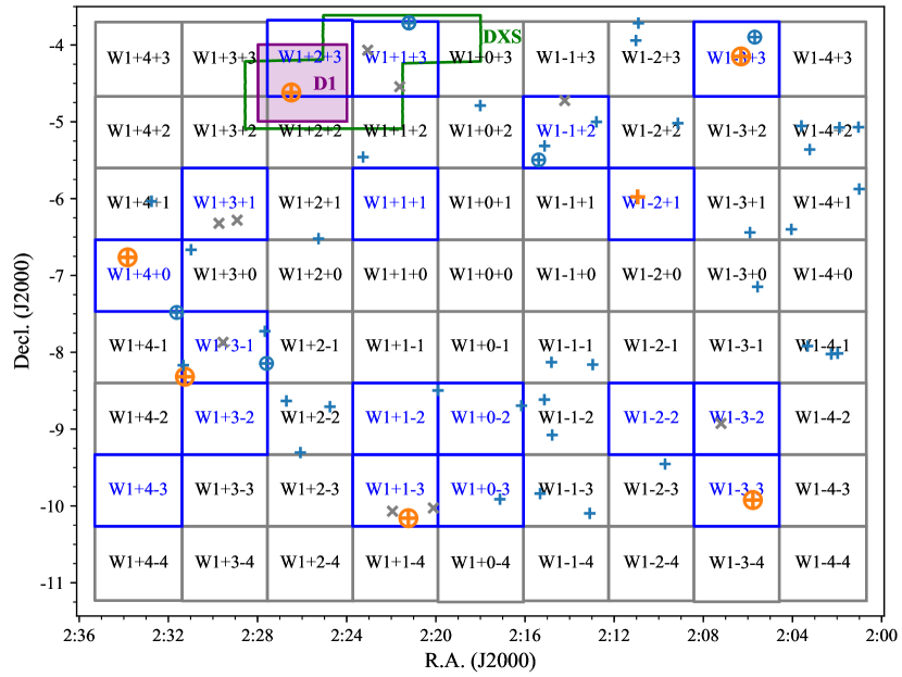
Figure 1: Layout of the CFHTLS W1 field. Individual Megacam pointings are labeled as in Gwyn (2012). Gray (blue) lines mark the boundaries of pointings rejected (accepted) by our field selection cuts for the faint candidate selection. The boundary of the UKIDSS DXS region is displayed with a green line, and the Deep D1 field as a filled purple square. The positions of our final quasar candidates are marked with plus signs, with blue (orange) indicating bright (faint) objects and circles drawn around objects with spectroscopy. Additional objects with spectroscopic observations not included in the final candidate list are marked with gray crosses.

2 CFHTLS imaging data

The CFHTLS Wide encompasses a total of 150 deg² split over four widely spaced fields. Stacked images and derived catalogs from the MegaPipe processing are publicly available on the CADC website and are described in Gwyn (2012). Not only are the CFHTLS Wide data considerably deeper than the Stripe 82 coadded imaging, they also have superior image quality. The stacked images have typical 5$\sigma$ magnitude limits of $r=25.9$, $i=25.7$, and $z=24.6$, and PSF FWHM $\sim$0.6-1.0″; compared to $i\approx 23.5$ and $\sim$1.0″ for Stripe 82.

We also utilize the CFHTLS Deep survey data. These consist of four independent, single MegaCam pointings (1 deg² in area) with depths of $i=27.4$. Two versions of the Deep image stacks are available: the “full-depth” coadds which utilize a larger number of input images, and the “best-seeing” coadds which are derived from a subset of images with the best image quality.

Image stacks for both the Wide and Deep data were generated by selecting input images based on quality criteria, resampling the images to remove geometric distortions, and combining them with a median algorithm using SWarp. The astrometric and photometric calibrations were obtained from comparison to SDSS measurements when available. The final catalogs were produced with SExtractor. Complete details of the MegaPipe processing are provided in Gwyn (2012). The layout of the W1 field can be viewed in Figure 1.

As demonstrated in Paper I, color selection of quasars at $z\sim 5$ is efficient owing to the separation between typical quasar colors at this redshift and the track defined by the stellar locus. However, this efficiency is extremely sensitive to the photometric accuracy, as the population of M dwarf stars similarly with red colors is several orders of magnitude more numerous than the high redshift quasar population. Furthermore, at increasingly faint fluxes unresolved galaxies with red colors begin to outnumber stars, particularly at high Galactic latitudes. For these reasons obtaining both an accurate photometric calibration and reliable star/galaxy separation from the CFHTLS imaging is crucial to this work.

We chose to generate our own photometric catalogs from the CFHTLS Wide images in order to better understand any systematic variations in the photometry and to improve the star/galaxy separation. These catalogs include PSF-based measurements using the PSF kernels obtained from PSFEx as part of the MegaPipe processing. Detection is performed on the $i$-band images and forced photometry is obtained in the other bands. We perform several diagnostic tests in order to assess the reliability of our photometric catalogs and to control for systematics in the CFHTLS imaging, as detailed in the following subsections.

2.1 Star/galaxy separation

An initial examination showed that the CLASS_STAR parameter provided in the CFHTLS SExtractor MegaPipe catalogs was not reliable in our magnitude range of interest ($i\gtrsim 23$). After exploring several approaches to this problem, we adopt a star/galaxy criterion similar to that employed by the SDSS. Namely, we use the difference between the flux measured with a PSF-shaped aperture and that measured through an elliptical Kron-like aperture (PSF_MAG and MAG_AUTO in SExtractor, respectively). This differs slightly from the SDSS definition, which uses the best-fit model magnitude instead of an elliptical aperture (where the model is selected from either a de Vaucouleurs or exponential disk profile, Stoughton et al. 2002), but we obtain acceptable results with this definition.

We examine the reliability of our star/galaxy separation with several test sets, paying particular attention to the performance at faint magnitudes. First, we use HST data from the CANDELS survey (Grogin et al. 2011; Koekemoer et al. 2011). The UDS ACS/F814W imaging has an area of $\sim 150$ arcmin² and lies within the CFHTLS-W1 field. We select 292 stars from the UDS v1.0 catalogs (Galametz et al. 2013) using F814W FWHM measurements. After matching the stellar objects to the CFHTLS Wide catalogs we find that the average $i$-band magnitude difference for stars with $i<24$ is $\langle i_{\rm AUTO}-i_{\rm PSF}\rangle=0.11$, with 89% (94%) of the UDS objects having $i_{\rm AUTO}-i_{\rm PSF}>0.0~{}(-0.1)$. Thus this method is highly complete at selecting stellar objects from the HST imaging; however, these results are based on a small region lying entirely within a single Wide pointing (W1+0+2) that has exceptionally good seeing (0.57″ in $i$-band) and may not be representative of the full survey.

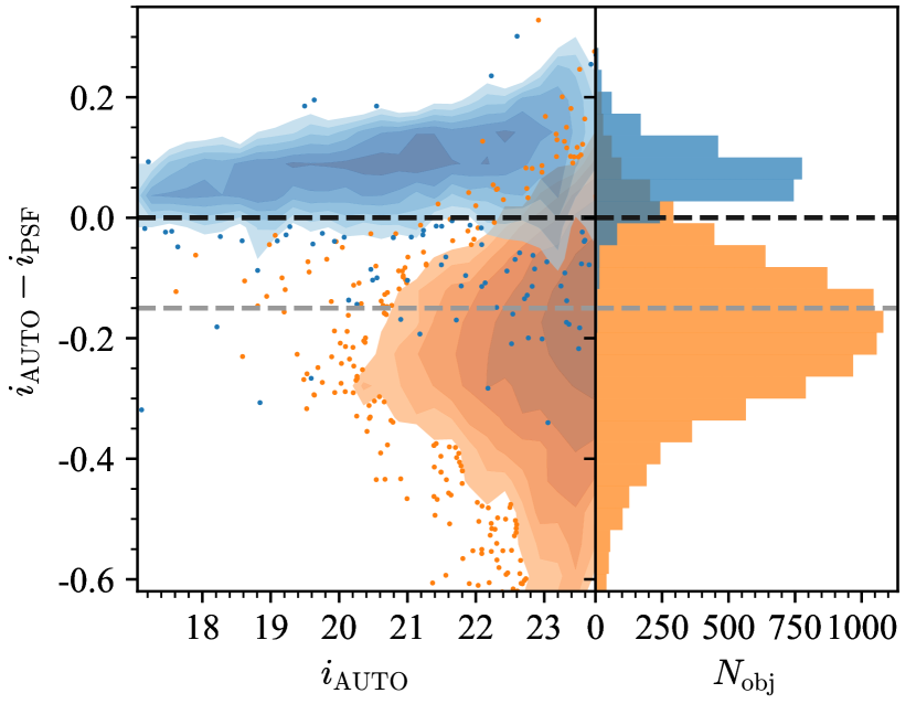
Figure 2: Demonstration of the star/galaxy separation cuts. The Deep D1 best-seeing catalogs are used as a reference. Stellar objects are selected from D1 using a cut on the half-light radius of $r_{1/2}<0.4$″. Compact galaxies are selected in the range $0.45$″$<r_{1/2}<0.55$″. Both samples are cross-matched to counterparts in the overlapping Wide catalogs. In the left panel the blue (orange) shaded contours and points represent the density of stellar (non-stellar) objects as a function of magnitude and MAG_AUTO$-$MAG_PSF. The right panel displays histograms of both samples. The black dashed line is the more strict cut used for the faint candidate selection, which is $\sim 88$% complete at $i_{\rm AB}\gtrsim 23$ while rejecting $>95$% of the compact galaxies. The more inclusive cut used for the bright candidate selection is displayed with a gray dashed line and is $\sim 98$% complete to faint stellar objects.

For a second test we use the Deep stacks from the CFHTLS. The Deep field D1 lies entirely within the Wide field W1 and overlaps with four individual Wide pointings. The D1 best-seeing stacks have an image quality of 0.64″ in the $i$-band, compared to 0.7-0.9″ in the overlapping Wide fields. We utilize the superior depth and resolution of the Deep data to identify stellar objects and then compare to the corresponding Wide photometry.

We use the MegaPipe D1 best-seeing catalogs to select stars from the locus of points in size-magnitude space. We find that the stellar locus is resolved from the galaxy distribution to a limit of $g\lesssim 23.7$. We use the $g$-band to select stellar objects, then examine their $i$-band photometry for classification. When the cut $i_{\rm AUTO}-i_{\rm PSF}>0.0~{}(-0.15)$ is applied to the Wide catalogs, 94% (99%) of the D1 stars are selected to a limit of $i=23.7$, in good agreement with the HST results. Focusing on the range $22.8<i<23.7$, the completeness is slightly lower, with the same cuts selecting 88% (98%) of the unresolved sources from D1. If we select compact galaxies by identifying marginally resolved sources with a measured size just above the stellar locus ($r_{1/2}\approx 0.5$″, compared to $r_{1/2}\approx 0.35$″ for stars), a cut of $i_{\rm AUTO}-i_{\rm PSF}>0.0$ eliminates $\sim 96$% of the compact galaxy contamination at $i\gtrsim 23$. The results of this test are presented in Figure 2.

Finally, we check these cuts against a sample of known quasars drawn from our spectroscopy of candidates in the CFHTLS. In early versions of our candidate selection weaker star/galaxy cuts were applied, resulting in greater contamination. Half of the non-quasars from our spectroscopic observations are rejected by an $i_{\rm AUTO}-i_{\rm PSF}>0$ cut.

We conclude from these tests that a cut of $i_{\rm AUTO}-i_{\rm PSF}>0.0$ is $\sim 90\%$ complete at selecting stellar objects from the Wide imaging, while greatly reducing the contamination from compact galaxies. We adopt this cut for selecting faint quasars, where the galaxy contamination is greater, while using the more permissive $i_{\rm AUTO}-i_{\rm PSF}>-0.15$ cut for brighter objects.

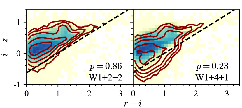
Figure 3: Examples of the stellar locus matching procedure used to select fields with greater photometric reliability. In both panels the background image represents the density of stars in $r-i$/$i-z$ color space in the Deep D1 field, with blue (yellow) indicating higher (lower) density. The dark red contours denote the stellar density in two different Wide pointings. The left panel presents a pointing that is an example of a good match to the Deep photometry, while the pointing in the right panel is a poor match. For reference, the black dashed line marks the color cut used to separate stars and quasars in Paper I; the pointing on the right has substantially greater contamination from stars scattered below this boundary.

2.2 Field selection

The expected density of $z\sim 5$ quasars with $i\lesssim 23$ on the sky is $\sim 1~{}{\rm deg}^{-2}$. Searching the full CFHTLS Wide area (150 deg²) would result in too many candidates to confirm spectroscopically given 30-60 min exposures for the faintest targets. We thus focus our attention on individual pointings within the CFHTLS that are likely to yield the highest reliability for color selection. In this section we detail the criteria used to select CFHTLS pointings in order to define our survey area. As described in Gwyn (2012), each pointing is a contiguous, $\sim 1~{}{\rm deg}^{2}$ area corresponding to a single MegaCam field-of-view, with a small overlap area between adjacent pointings.

First, we require homogeneous $i$-band filter coverage. During the course of the CFHTLS the $i$-band filter was replaced. The two filters used, $i^{\prime}_{1}$ and $i^{\prime}_{2}$, have significantly different profiles at the blue edge of the filter. As can be seen in Fig. 6 of Gwyn (2012), the $i^{\prime}_{2}$ filter has a peak $\sim 150$Å bluer than the $i^{\prime}_{1}$ filter. This shift has a substantial effect on quasar colors at $z\sim 5$, inducing differences of $\sim 0.1$–$0.2$ mag in the $r-i$ and $i-z$ colors between the two filters. As most of the CFHTLS was observed with the $i^{\prime}_{1}$ filter, we simply remove all fields with $i^{\prime}_{2}$ coverage from our survey in order to maintain a consistent set of selection criteria.

Next we select fields in order to optimize the photometric reliability. The five-band imaging for the CFHTLS was performed over a period of years, with varying conditions occurring in the individual images contributing to the final stacked images. This can lead to difficulties in obtaining an accurate representation of the coadded PSF, as well as non-uniform depths between the different bands.

To address the issue of non-uniform depth, we utilize the limiting depths for each pointing and each band given in Table 4 of Gwyn (2012). For our faint object selection criteria (defined in §3.4), we require that the limiting magnitudes (50% completeness) in the bluest and reddest bands are $g_{\rm lim}>26.3$ and $z_{\rm lim}>24.5$, respectively. These two bands are crucial in $z\sim 5$ quasar selection. The Lyman Limit for $z\sim 5$ quasars is redward of the $g$-band, thus relatively deep $g$-band imaging ensures that candidates are $g$-band dropouts. The $z$-band is typically much shallower than the $i$-band, but blue $i-z$ colors are an important discriminant between quasars and stars, and thus reliable $z$-band photometry is a necessity.

To further constrain the photometric reliability we assess the colors of objects along the stellar locus. Our approach is broadly similar to using principle colors to define a well calibrated stellar locus (Ivezic et al. 2004) or stellar locus regression (High et al. 2009). However, as we are only interested in selecting the best fields we do not attempt to improve the calibration (cf. Matthews et al. 2013, who discuss a recalibration of the CFHTLS data). We define the stellar locus using photometry from the Deep survey as a reference, and then compare photometry from individual Wide pointings to this reference using the binned maximum likelihood (ML) as a metric, where the data are binned in their $r-i$ and $i-z$ colors. Figure 3 presents examples of this method. The left panel contains a color-color plot from a “good” Wide pointing with colors well matched to the Deep catalogs. A poor match is presented in the right panel. The binned ML provides the probability of a match between the two distributions; based on examining the color-color plots we select a threshold of $p_{\rm locus}>0.52$, which removes $\sim 40$% of the W1 pointings. Imposing all of the quality cuts on W1 retains only 18/72 (25%) of the pointings in the full area; we will utilize this region for selection of the faintest candidates (§3.4).

3 Target selection

3.1 Simulated quasar colors

As in Paper I, our target selection is guided by models for quasar colors at $z\sim 5$. The paucity of known quasars at this redshift means that a limited training set is available, we thus generate simulated quasar colors trained on the properties of the more abundant quasar population at lower redshift, assuming that quasar spectra do not strongly evolve (e.g., Kuhn et al. 2001; Jiang et al. 2006). Specificially, our model is derived from the observed spectral properties of SDSS BOSS DR9 quasars (Ahn et al. 2012; Ross et al. 2013), which capture the UV emission of $\sim 150,000$ quasars at $z\sim 2.5$ over a wide luminosity range. The model includes a broken power law continuum, an emission line template capturing the Baldwin Effect (Baldwin 1977), iron emission templates (Boroson & Green 1992; Vestergaard & Wilkes 2001; Tsuzuki et al. 2006), and a stochastic IGM HI absorption model (Worseck & Prochaska 2011; McGreer et al. 2013). Quasar spectra are generated though Monte Carlo samplings of the individual spectral features in order to reproduce the intrinsic scatter in colors at any given redshift. The simulated spectra are then convolved with filter bandpasses to produce mock photometry, and then realistic scatter is introduced to mimic actual observations. The code to generate simulated quasar spectra and photometry is written in Python and is freely available; additional details of its implementation are provided in Paper I and Ross et al. (2013).

Figure 4: Simulated quasar colors in $riz$ color space. The simulations include 140,000 objects in the range $4.3<z<5.8$. The color scale indicates the mean redshift in bins of width $0.07$ mag in $riz$ colors. The location of the stellar locus is given by logarithmically stepped contours represented by dark gray lines. The color selection efficiency peaks at $z\sim 5.0$ as the colors of typical quasars separate from the stellar locus.

We adopt the model parameters used in Paper I, but update the model to include photometry in the CFHT MegaCam system with photometric errors appropriate for the CFHTLS Wide survey. Results of the simulations are presented in Figure 4, demonstrating that for our fiducial quasar model the $riz$ colors of $z\sim 5$ quasars are well separated from the stellar locus.

3.2 Color selection

The color criteria presented in Paper I were designed for quasar selection in Stripe 82 and require modification for the present work: although the CFHT photometric system is quite similar to the SDSS, the differences are sufficient to result in markedly different colors of $z\sim 5$ quasars (of order $\sim 0.2$ mag). We adopt the following color cuts for the CFHTLS Wide selection:

$$S/N(u)<2.2~{}~{},$$ (1)

$$g-r>1.8~{}~{}{\rm OR}~{}~{}S/N(g)<2.2~{}~{},$$ (2)

$$r-i>1.3~{}~{},$$ (3)

$$i-z<0.15+0.875[(r-i)-1.3]~{}~{},$$ (4)

$$i-z<0.5~{}~{}.$$ (5)

We refer to these cuts at the “strict” color criteria.

Alternatively, we also consider “weak” criteria defined by replacing equations  4  and  5 with:

$$-0.5<i-z<0.55~{}~{}.$$ (6)

The weak criteria are highly complete but by themselves result in an unacceptably high level of contamination. These criteria will be used when ancillary data is available to reduce the contamination.

In Paper I we utilized near-IR imaging from UKIDSS to assist in rejecting stars. The CFHTLS Wide fields are not uniformly covered by sufficiently deep near-IR imaging to aid in quasar candidate selection. Alternative means of expanding on optical color selection, e.g., through radio (McGreer et al. 2009) or mid-IR (Wang et al. 2016) data were similarly not available to sufficient depth and area in these fields. We thus found it desirable to prioritize the color-selected candidates with a probabilistic approach.

3.3 Likelihood selection

We adopt the likelihood method (Kirkpatrick et al. 2011) to rank our candidates and to provide additional candidates missed by the color cuts. This method requires a training set of quasars (“QSO”) in the desired redshift range, and a catalog of non-quasar contaminants (“Everything Else“, or EE). After properly normalizing the training set catalogs, quasar probabilities are assigned to input objects by asking whether they are more likely to belong to the QSO or EE catalogs. The relative probabilities are obtained from a $\chi^{2}$ statistic calculated by comparing the input fluxes and errors to the training set fluxes in a multidimensional space.

The likelihood method has the limitation of including photometric errors in the training sets (see Bovy et al. 2011 for a related method that avoids this issue). We mitigated this problem by using the CFHTLS Deep survey catalogs, which have substantially smaller photometric errors than the Wide catalogs, for our EE training set and the (noise-free) simulated quasar photometry for our QSO training set. The simulated quasars were necessary as no training set of known quasars at $z\sim 5$ with similar fluxes as our targets exists.

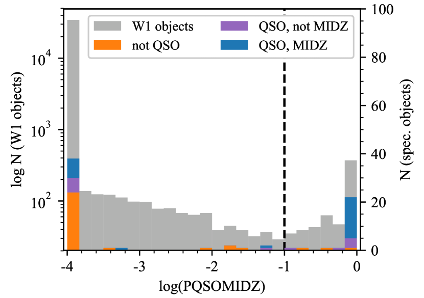
Figure 5: Distribution of log-likelihoods that objects are quasars at $4.8<z<5.2$ (${\rm\tt PQSOMIDZ}$). The gray histogram is constructed from the W1 pre-selected object catalog (§3.3) and is shown on a logarithmic scale (left axis). The number of objects with spectroscopy is tallied as orange (non-quasars), purple (quasars not in mid-$z$ range), and blue (quasars in the mid-$z$ range) bars on a linear scale given on the right axis. A lower bound of $10^{-4}$ is set on the probabilities. A cut of ${\rm\tt PQSOMIDZ}>0.1$ is used to select candidates with the likelihood method.

EE catalog: The Everything Else catalog was constructed from the $i$-band detection catalogs derived from the full-depth Deep coadds. The Deep field photometry is in an identical system as the Wide field, but the photometric uncertainties are negligible in our range of interest. On the other hand, the Deep fields cover a much smaller area and have a limited sampling the full distribution of contaminants, particularly at the bright end.

We first restrict the catalog to the unmasked survey regions, resulting in 1.5 million objects. We then remove objects with suspect photometry (I_FLAGS=0 from SExtractor), and apply a cut on stellarity. Formally, our likelihood model could include the probability that a candidate object is a star, and thus fold in the stellar probability for objects in the EE catalog. We instead take the simpler approach of applying the star/galaxy cut $i_{\rm AUTO}-i_{\rm PSF}>-0.15$ to the Deep photometry. We account for inaccuracy in the star/galaxy classification by including a random sampling of objects from the Deep catalogs that pass the stellarity cut based on their Wide measurements but not with the Deep photometry. The final EE catalog has 600,000 entries and an effective area of 3.3 deg².

QSO catalog: The mock quasar catalog is constructed from the simulations. First, we distribute a sample of quasars in luminosity and redshift according to the luminosity function from Paper I (row 1 in Table 5). The total number matches the expectation for a survey with an area of 250 deg², roughly twice the area we searched in CFHTLS, and the sample is bounded by $M_{1450}<-21.9$ ($i_{\rm AB}<24.2$ at $z=5$) and $4.5<z<5.8$.

We generate simulated spectra and photometry as described in §3.1. Although the simulated photometry is noiseless, this approach is limited by any systematic errors in our quasar model. The model has been shown to accurately reproduce the colors of SDSS BOSS quasars at $2.2<z<3.5$ (Ross et al. 2013), and we assume it applies equally well to $z\sim 5$ quasars. Following Bovy et al. (2011) we divide the simulated quasars into three redshift bins in order to gain information about objects likely to be just below or above our target redshift range. The probabilities are calculated as $p(f_{i},z_{1}\leq z<z_{2}~{}{\rm quasar})$ where $f_{i}$ represents the (linear) fluxes in the five SDSS bands and the three redshift bins are ${\rm\tt PQSOLOWZ}$ ($4.5<z<4.8$), ${\rm\tt PQSOMIDZ}$ ($4.8<z<5.2$), and ${\rm\tt PQSOHIZ}$ ($5.2<z<5.8$). We also calculate the summed probability that an object is in the full redshift range (${\rm\tt PQSO}$). Quasars outside of this redshift range are ignored; they will contribute negligible contamination given our color cuts, and are implicitly included in the EE catalog.

With our training sets in hand we now derive quasar probabilities for objects in the Wide catalogs. To ease the calculation we only compute likelihoods for objects with I_FLAGS=0, $i<24$, $g-r>1.5$, and $r-i>1.0$. These criteria are unlikely to miss any quasars at $z\sim 5$ and reduce the input list to $\sim$100,000 objects in the four CFHTLS-Wide fields. Figure 5 presents the distribution of likelihoods for the pre-selected list in the W1 field. The vast majority have ${\rm\tt PQSOMIDZ}<10^{-4}$. The choice of ${\rm\tt PQSOMIDZ}\gtrsim 0.1$ roughly picks out a minimum in the distribution separating the likely quasars from the stellar contaminants. We thus apply the cut

$${\rm\tt PQSOMIDZ}>0.1$$ (7)

to define “likelihood-selected” candidates.

3.4 CFHTLS Wide targets

The final target selection is obtained from a combination of the color and likelihood selection methods. We define three distinct samples of targets. First, we select bright candidates ($i_{\rm AB}<23.2$) in the W1, W3, and W4 fields. In the W4 field we only considered pointings that overlap with the SDSS Stripe 82 imaging in order to prioritize candidates that are in common with the Paper I sample. The bright targets provide backup targets for observing runs with sub-par conditions, and an independent sample that spans the luminosity range of the Paper I QLF, while also extending 1 mag deeper.

Figure 6: Colors of high redshift quasars and stars in CFHTLS-W1. The gray contours and points represent the density in logarithmic steps of catalog objects with $i_{\rm AUTO}-i_{\rm PSF}>-0.15$ and to a depth of $i_{\rm AB}<23.2$. The solid (dashed) magenta line marks the boundaries of our strict (weak) $riz$ color selection criteria. Objects in the bright candidate sample are represented by filled blue pentagons for spectroscopically confirmed quasars, orange stars for non-quasars, and empty purple circles for objects without spectroscopic observations. Objects with spectroscopy not included in the final sample are represented by green pluses for quasars in the redshift range $4.7<z<5.3$, green crosses for quasars outside of that redshift range, and yellow crosses for non-quasars.

For the bright targets we ignore the field selection criteria from §2.2 and select candidates with both the strict color criteria from §3.2 and the likelihood selection from §3.3 (i.e., a candidate may be selected by either method). We apply a highly inclusive star/galaxy cut of $i_{\rm AUTO}-i_{\rm PSF}>-0.15$, which is $\gtrsim 99$% complete to stellar objects (§2.1). Finally, we visually inspect the candidates and discard spurious objects and those with unreliable photometry.

Applying these criteria to the W1, W3, and W4 fields yields 97 candidates over an area of 105 deg², after removing 22 during the visual inspection step. The strict color criteria select 87 of the candidates, the likelihood criteria 55, and 45 candidates pass both criteria. Only 10 of the candidates lie outside of the color boxes and are selected by likelihood only; all of these targets lie within the weak color criteria. The full list of bright candidates is provided in Table 4; a visualization of the color selection of the bright targets is presented in Figure 6.

Next we define the faint quasar sample in the W1 field, selecting quasar candidates with $23.2<i_{\rm AB}<23.7$. For the faint targets we apply the field selection criteria to identify the most reliable pointings within W1, and we apply a stricter star/galaxy cut of $i_{\rm AUTO}-i_{\rm PSF}>0.0$. This results in seven candidates from an area of 18.5 deg², after removing two objects by visual inspection. These objects provided the primary target list for the Gemini observations. The candidate list is provided in Table 5. A color-color plot of the faint candidates is presented in Figure 7, showing that all seven meet the strict color criteria.

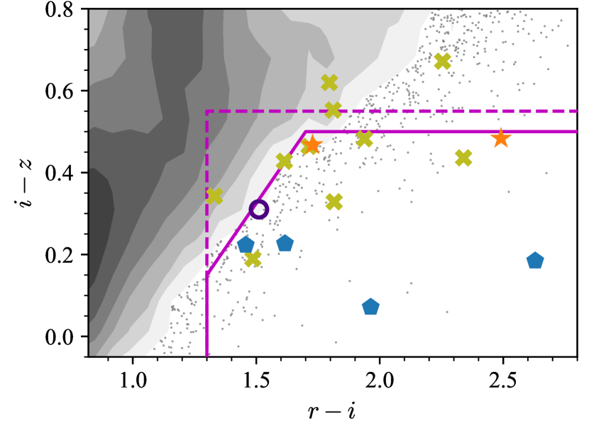
Figure 7: Same as in Fig. 6, but for the faint targets in W1. The background contours represent W1 objects with $23.2<i_{\rm AB}<23.7$ and $i_{\rm AUTO}-i_{\rm PSF}>-0.15$; note that the distribution has a somewhat different shape than for the brighter objects likely due to a larger contribution from compact galaxies. A few objects that lie outside the color boxes were observed with Gemini because they were selected as backup targets based on aperture photometry; none of these were found to be quasars. Additionally, none of the backup targets selected by colors but with low likelihood values were quasars.

3.5 Ancillary selection in D1+DXS

Our candidate selection from the CFHTLS-Wide is complemented by deep data from two ancillary regions. First, the Deep D1 field lies entirely within the Wide W1 field, spanning one square degree and overlapping with four separate Wide pointings. The D1 $i$-band data are $\approx 1.6$ mag deeper on average than the overlapping Wide pointings, and the image quality of the best-seeing stack is 0.64″, compared to $<{\rm IQ}(i)>=0.73$″ for the Wide images.

Second, the W1 field is partially covered by near-infrared imaging from the UKIDSS Deep Extragalactic Survey (DXS). As shown in Paper I, near-IR photometry is highly useful for rejecting stellar contaminants in $z\sim 5$ quasar selection, as stars have redder $i-J$ colors than quasars with similar optical colors. At the time of our observations, the DR9 release from UKIDSS provided $2.52~{}{\rm deg}^{2}$ of $JK$ imaging within the W1 field to depths of $J_{\rm AB}\approx 23.2$ and $K_{\rm AB}\approx 22.6$ ($5\sigma$). An area of 0.88 deg² within DXS overlaps with D1 (see Fig. 1).

We first search within the DXS region by applying the weak color criteria from §3.2 to the W1+DXS overlap area. We remove all cuts on morphology, photometric flags, and imaging masks. We then apply the following near-IR criteria, similar to those used in Paper I:

$$i-J<((r-i)-1.3)+0.8~{}~{},$$ (8)

$$i-J<1.2~{}~{},$$ (9)

after substituting a nominal detection limit for the $J$-band non-detections. These cuts select 14 candidates with $23.2<i<23.7$, of which six are within D1. Examining the D1 photometry for those six objects, we find that with the deeper photometry all but one fail the weak color criteria, and thus are not likely to be $z\sim 5$ quasars.

We additionally search the 0.88 deg² D1+DXS overlap region using the D1 photometry as input to the weak color criteria. This test would identify objects with quasar-like colors scattered outside of the color boxes in the shallower Wide imaging. This search yields only two candidates, both of which were also selected by the W1+DXS search.

One of the two D1+DXS color-selected candidates has $i_{\rm AUTO}-i_{\rm PSF}=-0.4$ in the D1 best-seeing catalogs. This object is clearly elongated in the $i$-band best-seeing image and its radial profile is more extended than the profiles of nearby stars. Thus we reject it as a quasar candidate, and retain a single good candidate from the D1+DXS area. This candidate is a confirmed $z=4.9$ quasar (§4).

We also test somewhat more restrictive near-IR color cuts:

$$i-J<0.75((r-i)-1.3)+0.7~{}~{},$$ (10)

$$i-J<1.0~{}~{}.$$ (11)

This reduces the W1+DXS sample to two objects. One is the quasar also identified in the D1+DXS search. The other is also in D1 but falls outside of the weak color cuts when using the D1 photometry. The fact that nearly all of the W1+DXS candidates selected with relaxed optical color criteria applied to the Wide photometry are rejected either by the more restrictive near-IR cuts and/or by using deeper optical photometry suggests that they are unlikely to be quasars.

In summary, the D1 and DXS data demonstrate that our selection criteria from the Wide survey are not missing a significant number of valid candidates just outside the selection boundaries. Even after applying highly permissive color criteria to the Deep catalogs, we identify only a single quasar candidate in the D1 area. This corresponds to a sky density of $0.40~{}{\rm deg}^{-2}$, in excellent agreement the result from the Wide fields over the same magnitude range, $0.39~{}{\rm deg}^{-2}$. We kept a small number of the W1+DXS-selected candidates in our target list but at a low priority for observations.

4 Spectroscopic Observations

Figure 8: Spectra of CFHTLS quasars observed with GMOS at Gemini North. The spectra have been smoothed with a $\sim 12$Å boxcar. Vertical tick marks indicate the location of typical quasar emission lines, from left to right Ly$\beta$, Ly$\alpha$, N V, O I, Si IV, and C IV. CFHTLSJ020541-035350 is not included in the final candidate sample, and CFHTLSJ023349-064551 is an example of a non-quasar. The spectra generally display broad emission lines typical of luminous quasars, as well as BAL-like absorption features near the wavelengths of N V, Si IV, and C IV.

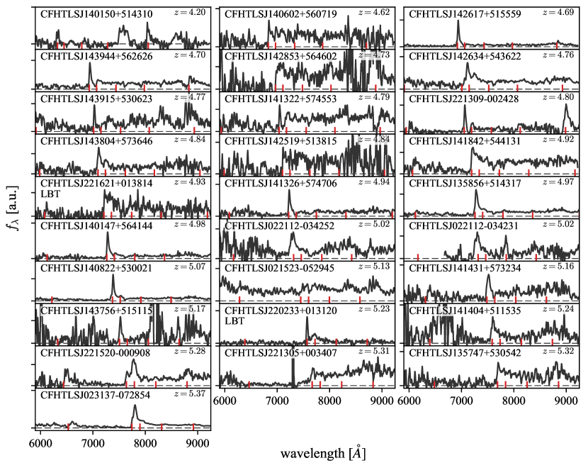
Figure 9: MMT Red Channel spectra of CFHTLS quasars (the two spectra from LBT are labeled under the object names). Redshifts are obtained from template fitting; however, given the low quality of the spectra and the strong absorption features, the redshifts are only accurate to $\Delta{z}\sim 0.1$. The same emission lines as in Fig. 8 are denoted with vertical red marks. CFHTLSJ021523-052945 has a noisy extraction but the Ly$\alpha$+N V feature is apparent in the 2D spectrum.

4.1 Gemini-North

We obtained spectroscopic observations of faint quasar candidates from CFHTLS-W1 using GMOS on Gemini North through classical mode observations conducted on 2013 October 24-25 (program GN-2013B-C-1). Conditions were excellent with 0$\farcs$4-0$\farcs$6 seeing throughout. Spectra were obtained through a 1″ longslit and dispersed with the R400 grating, yielding a resolution of $R\sim 1000$. The grating was centered at 7400 Å and the OG515 blocking filter was used; this setup provides coverage from 5320 Å to 9500 Å. The e2V detectors were binned by a factor of two in both the spatial and spectral directions, resulting in a spatial scale of 0.15 arcsec pix^-1 and a dispersion of 1.34 Å pix^-1. Each target was observed with a single 1200s integration; based on an assessment of the 2D spectrum additional exposures were sometimes obtained to increase the $S/N$. No dithering in either the spatial or spectral directions was performed between successive exposures. We observed a total of 17 targets, including all four of the likelihood candidates.

Data were processed in a standard fashion using the IRAF gemini.gmos package. After bias subtraction and flat field correction, cosmic rays were identified and masked using the LACOS (van Dokkum 2001) routines. The 2D images were then stacked using gemcombine. The targets are faint and the per pixel $S/N$ is quite low; we thus extracted 1D spectra by following a reference trace obtained from observations of bright quasars taken each night as part of another program. Wavelength calibration was provided by CuAr lamps. The spectra were flux-calibrated using observations of the spectrophotometric standards Wolf 1346 and Hiltner 600 obtained once per night.

The Gemini observations resulted in five newly confirmed quasars at $4.5<z<5.4$ with a typical magnitude of $i=23.5$. The final spectra are displayed in Figure 8. The Ly$\alpha$ line is readily apparent in each case. The 12 non-quasars present only featureless continua; they could be either late-type stars or faint red galaxies. An example spectrum of a failed target (non-quasar) is given in Fig. 8. Matsuoka et al. (2017) have presented observations of $z\sim 6$ quasar candidates at a similar luminosity selected from Subaru Hyper Suprime-Cam (HSC) imaging, and find a large number of sources with narrow Ly$\alpha$ emission and no obvious quasar emission lines, or with galaxy-like spectra. Some of our failed quasar targets may indeed be absorption line galaxies with no strong emission features, but the spectra are of insufficient quality to establish their redshift and type.

4.2 MMT

We observed a large number of candidates with the 6.5m MMT using the Red Channel spectrograph during a number of observing runs from 2012 to 2014. The MMT targets were primarily selected as backup targets for poor observing conditions and were limited to $i<23$. One run from 2012 May 27-28 was dedicated to this program and conditions were excellent during this run with 0$\farcs$7 seeing; we utilized this time for fainter targets ($i\sim 23$).

We observed quasar candidates with the low dispersion 270 mm^-1 grating, typically centered at 7500 Å with coverage from 5500Å to 9700Å. We alternated between the 1″ or 1.5″ slit based on the seeing, providing resolutions of $R\sim 640$ and $R\sim 430$, respectively.

Data processing employed standard longslit reduction methods using scripts written in Python and using Pyraf routines. Basic corrections included bias subtraction, pixel level flat fields generated from internal lamps, and sky subtraction using a polynomial background fit along the slit direction. Cosmic rays were identified and masked using the LACOS routines (van Dokkum 2001). Initial wavelength solutions were obtained from an internal HeNeAr lamp and then corrected using night sky lines (primarily the OH line list given by Rousselot et al. 2000); the final RMS for sky lines is $\sim 2$Å. Spectrophotometric standard stars were observed each night and used for flux calibration. However, the conditions were generally variable and the absolute flux calibrations are only approximate.

The MMT sample also includes five targets from Stripe 82 that did not have spectroscopy at the time Paper I was prepared. These objects are listed in Table 3 in the Appendix.

Several of the targets observed with MMT have unusual properties. Two quasars, CFHTLS J022112.3-034231 and CFHTLS J022112.6-034252, form a small-separation (20″) binary quasar at $z=5.02$; constraints on quasar clustering at $z\sim 5$ derived from this pair are discussed in McGreer et al. (2016). Another target, CFHTLS J141446.8+544631, is in our final quasar candidate sample but is a $z=5.42$ lensed galaxy with strong Ly$\alpha$ emission. Additional spectroscopy and multiwavelength observations of this object are presented in McGreer et al. (2017). Finally, CFHTLS J141956.4+555316 is tentatively assigned a redshift of $z=5.0$ based on a marginal line detection at $\sim 7310$Å. The line appears in multiple sky-subtracted 2D spectra, but extraction is hampered by a strong complex of OH airglow lines at these wavelengths. This object may be a weaker version of CFHTLS J141446.8+544631 but needs deeper spectroscopy to confirm its nature.

4.3 LBT

We obtained spectroscopy with the Large Binocular Telescope (LBT) Multi-Object Double Spectrograph (MODS1) instrument on 2012 September 21. MODS provides moderate resolution optical spectroscopy (Pogge et al. 2006). The primary target was a Stripe 82 quasar from Paper I that has a close companion galaxy; however, we also observed five CFHTLS-W4 candidates based on an early version of the target selection. Details of the observations can be found in McGreer et al. (2014); briefly, we used a 1″ slit in good seeing conditions ($\sim$0.8″) with the G670L grating ($R\sim 1400$), integrating for $\sim 30$min on each target.

Only two of the five targets are $z\sim 5$ quasars, and they are the only two objects which appear in the final candidate list.

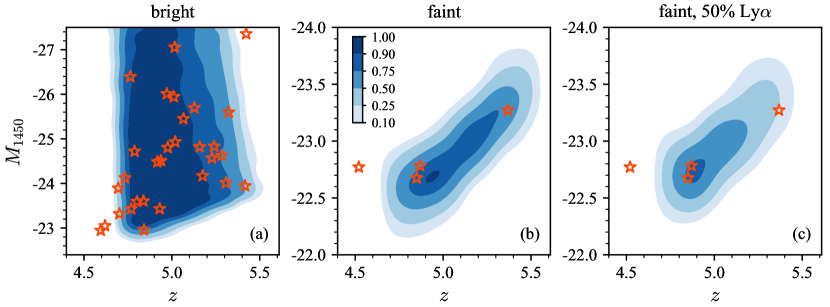
Figure 10: Selection functions for the color selection criteria (§3.2). The filled contours represent the selection efficiency with the scale given in panel (b). The completeness for the bright selection ($i_{\rm AB}<23.2$) is presented in panel (a), and for faint selection ($23.2<i_{\rm AB}<23.7$) in panel (b). Panel (c) presents results for the faint criteria applied to a quasar model with the assumed Ly$\alpha$ EWs reduced by half. The dependence of the selection on Ly$\alpha$ strength is further discussed in the Appendix. Spectroscopically confirmed quasars from the final candidate list are marked with red stars. The $z=4.5$ faint quasar that lies well outside the selection region is not formally likelihood-selected or color-selected, but observed because it has ${\rm\tt PQSOMIDZ}>0.01$.

4.4 Redshift determination

The spectra typically have modest $S/N$ ($\sim$few per pixel in the rest-UV continuum) and often the only well-detected feature is the Ly$\alpha$ emission line and the continuum break due to the onset of the Ly$\alpha$ forest. We obtain redshifts by fitting a set of templates to the spectra and varying the template redshifts, finding the best-fit through a $\chi^{2}$ minimization. The set of templates includes a fiducial quasar with emission line strengths and average forest absorption as generated by our models (§3.1) for a quasar with $M_{1450}=-24$. We also modify this fiducial template by reducing the more prominent UV emission lines by a factor of two, and add two narrow-line templates for which the broad components of the UV lines are set to zero and the narrow Ly$\alpha$ and C IV lines are either twice or half their nominal values from the models. Finally, we add a continuum-only template to represent a weak-lined quasar. Given that the templates are mainly fitting the Ly$\alpha$ feature the systematic uncertainty is $\Delta{z}\sim 0.1$.

The $k$-corrections are also determined from the quasar models, accounting for luminosity dependence (the Baldwin Effect) as in Paper I. The $i$-band magnitudes and redshifts are matched to model quasar spectra and used to determine the rest-UV continuum luminosity $M_{1450}$. Dust extinction is not included in these models.

5 Results

We obtained a total of 80 spectra of objects in the CFHTLS fields, with 17 spectra from Gemini, 61 from MMT, and 2 from LBT. Redshifts for two additional sources come from the BOSS DR9 quasar catalog (Paris et al. 2012). The complete sample of bright candidates includes 97 targets in W1+W3+W4 with $i<23.2$ (Table 4), of which over a third (39) have spectroscopic observations. This includes 38/87 (44%) of the color-selected candidates and 24/55 (44%) of the likelihood-selected candidates. The efficiency is quite high: 35/39 of the targets are $z>4$ quasars. For the faint W1 sample (Table 5), 6/7 were observed with Gemini/GMOS, including all of the likelihood-selected candidates (5), and 4/6 are $z\geq 4.6$ quasars.

5.1 Completeness

5.1.1 Color models

We determine the completeness of our selection criteria by using the color simulations to generate model quasar colors. The fraction of simulated quasars passing our color cuts is then calculated as a function of redshift and luminosity. This fraction is measured in a grid with bin widths ($\Delta{M}_{1450}$, $\Delta{z}$) = (0.1, 0.05) and with 100 quasars in each bin. Only the color criteria are considered this calculation. Although the likelihood method was used to prioritize candidates, the color and likelihood methods have an equal amount of spectroscopic coverage. The color-selected sample also provides a more well defined boundary for the selection cuts, especially considering that the same quasar model we use for the completeness calculation was used to train the likelihood model.

Figure 10 displays the selection function for the bright and faint quasar samples in the CFHTLS Wide survey. We derive photometry from our quasar models by including a representation of the CFHT photometric system with flux errors that match the depth of the Wide survey fields. We also update the completeness calculation of the SDSS DR7 and Stripe 82 quasar samples from Paper I. The new calculation fixes an error in $k$-correction used in Paper I that resulted in a shift of $\sim 0.1$ mag in the absolute magnitudes.

For consistency, the quasar color models used here (§3.1) are identical to those from Paper I and from the calculation of the luminosity function of BOSS quasars at $2<z<3.5$ (Ross et al. 2013). In Paper I we considered the effect of the Ly$\alpha$ emission on $z\sim 5$ quasar selection, noting that due to the Baldwin Effect we expect fainter quasars to have stronger line emission and thus be more easily selected by their redder $r-i$ colors (Ly$\alpha$ is in the $i$-band). However, if the properties of $z\sim 5$ quasars are different than the $z\sim 3$ quasars from BOSS used to calibrate our model, this would affect our completeness estimation. Panel (c) of Figure 10 compares the selection function derived for a model where the Ly$\alpha$ flux is decreased by a factor of two compared to the reference model (Panel b). Although the efficiency is reduced, particularly at $z\gtrsim 5$, the overall effect is rather modest and thus would not substantially alter the luminosity function results. In the Appendix (§7) we explore the dependence of the selection function on the assumed Ly$\alpha$ emission in greater detail and conclude that, although our color selection is less sensitive to quasars with weak line emission, it is unlikely we are missing a substantial population at $z\sim 5$.

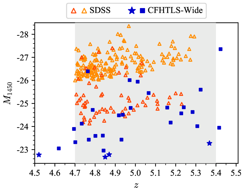
Figure 11: Distribution of the quasar samples in absolute UV magnitude and redshift. The updated results from SDSS DR7 (orange) and Stripe 82 (dark orange) are shown as empty triangles, truncated at $z>4.7$. The new CFHTLS quasars from the bright (blue squares) and faint (blue stars) candidate samples overlap with the Stripe 82 results from Paper I, but reach $\sim 1.5$ mag deeper.

5.1.2 Results from spectroscopy

The results from the Gemini spectroscopy provide validation of the likelihood method as applied to the faint candidates: all four targets assigned the highest priority — based on ${\rm\tt PQSOMIDZ}>0.1$ — were confirmed as $z>4.5$ quasars. Of the three additional targets selected with the strict color cuts but not likelihood, two were observed and neither were quasars.

In addition to the primary sample of seven color+likelihood targets, the favorable observing conditions permitted observations of lower priority targets just outside of the color selection boundary. Only one of these 11 targets is a quasar: J020541.5-035350 has $i=23.16$ and is included in the bright sample. With a redshift of $z=4.6$ it is just below the target redshift range, which agrees with the crude photo$-z$’s provided by likelihood: it has ${\rm\tt PQSOMIDZ}=0.06$ and ${\rm\tt PQSOLOWZ}=0.91$. The highest redshift quasar in the complete sample at $z=5.38$ has ${\rm\tt PQSOMIDZ}=0.10$, just at the threshold, but ${\rm\tt PQSOHIZ}=0.90$.

Many of the spectra for the bright candidates ($i<23.2$) were obtained before our selection criteria were finalized and thus probe regions outside of our selection boundaries. Of the 40 bright objects with spectroscopy not included in the final sample, 30 are not quasars and only eight are in the range $4.7<z<5.4$. Of those eight, five are relatively bright quasars ($i_{\rm AB}\lesssim 21$) that fail the rather stringent “dropout” criteria in the $u$ and $g$ bands (eqns. 1 and 2), and the other three are just outside the color cuts. These three objects have redshifts near the edges of our bin ($z=4.701,5.228,~{}{\rm and}~{}5.364$) where the selection efficiency is lower. This provides further confidence in the completeness of our final selection criteria. The likelihood cut also misses eight quasars in the mid-$z$ range (see Fig. 5), but again most of the missed quasars are near the edge of the redshift bin.

5.2 Photometric and Spectroscopic Completeness

At the depths probed by our survey the CFHTLS imaging is highly complete. By comparing the Wide survey catalogs to the overlapping Deep regions, we find that the Wide imaging recovers $\sim 96$% of stellar sources in the Deep best-seeing stacks at $i_{\rm AB}<23.7$, where most of the losses are due to blending with nearby sources. Additionally, as discussed in §2.1, our star/galaxy separation method is $\sim 90$% ($\sim 98$%) complete to point sources for the faint (bright) sample. Thus we estimate the photometric completeness to be 86% for the faint sample and 94% for the bright sample.

For the bright ($i_{\rm AB}<23.2$) quasar selection, we have obtained spectra for all targets with $i_{\rm AB}\leq 20.8$, 86% of the targets with $20.8<i_{\rm AB}\leq 22.6$, and 37% of targets with $22.6<i_{\rm AB}\leq 23.2$. For the faint quasar selection we have Gemini spectra for 6/7 targets. Both the photometric and spectroscopic completenesses are applied during the calculation of the luminosity function.

5.3 Binned Luminosity Function

The binned QLF is determined separately for three samples: “SDSS Main” consists of quasars from SDSS DR7. There are slight differences between the results presented here and those from Paper I due to the updated $K$-corrections and completeness models; otherwise, the observed sample of quasars is identical. “SDSS Stripe 82” is similarly updated from Paper I, but includes the five additional quasars with spectroscopic observations presented here. Finally, “CFHTLS Wide” consists of the results from the spectroscopic observations of targets in the CFHTLS Wide fields, including both the MMT, LBT, and Gemini observations of $i<23.2$ targets and the Gemini observations of $23.2<i<23.7$ targets. Although the selection methods for each of the three samples are slightly different, the quasar models and methodology used to calculate the completeness corrections are identical.

The nominal CFHTLS selection function extends to slightly higher redshifts than the SDSS and Stripe 82 samples from Paper I. We thus adopt a wider redshift bin of $4.7<z<5.4$ for the CFHTLS data, compared to the $4.7<z<5.1$ bin that was used in Paper I. However, we continue use the smaller bin for the recalculation of the SDSS and Stripe 82 QLF. The choice of a larger bin includes more of the quasars found in CFHTLS, but has little effect on the luminosity function as the number density declines steeply with redshift and the mean quasar redshift is $\langle{z}\rangle\approx 4.9$ for all three samples.

The results of the binned QLF calculation are given in Table 1. To calculate $\sigma_{\Phi}$ we have adopted the approximation for confidence intervals in the low count regime provided by Gehrels (1986). Figure 12 presents our measurement of the QLF over a dynamic range in luminosity greater than a factor of 100, to the limit of $M_{1450}=-22.9$ achieved with the faint CFHTLS quasars.

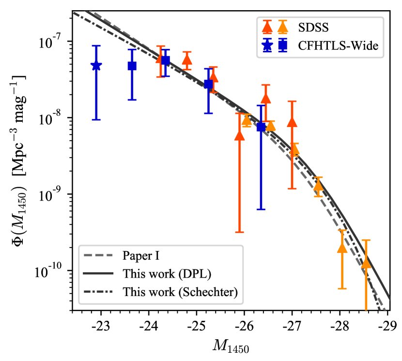
Figure 12: Binned QLF results at $z\sim 5$ shown as points with error bars, including the SDSS Main (orange), SDSS Stripe 82 (dark orange), and CFHTLS-Wide (blue) samples. The lines denote model fits to the QLF using maximum likelihood. The dashed line is the best-fit from Paper I using SDSS data only, the solid line is the best-fit double power law model from this work, and the dot-dashed line the best-fit Schechter function model. The Stripe 82 and CFHTLS points show good agreement where they overlap in luminosity. The faintest bin from the CFHTLS, based on the W1 Gemini spectroscopy and represented by a star, is well below the best fit QLF models.

The results from the CFHTLS fields agree well with those from SDSS Main and Stripe 82 in the luminosity range over which they overlap. Although the color selection methods used to target quasars in these surveys share a high degree of similarity, the input imaging data is quite different, providing some encouragement that the results are not sensitive to the systematics of any one survey.

Table 1: Binned QLF

$M_{1450}$	$N$	$N_{\rm cor}$	$\log\Phi$	$\sigma_{\Phi}$
SDSS Main
-28.55	1	1.7	-9.90	0.12
-28.05	2	2.6	-9.70	0.14
-27.55	13	17.2	-8.89	0.37
-27.05	34	51.5	-8.41	0.72
-26.55	67	100.4	-8.10	1.08
-26.05	30	38.6	-8.03	1.74
SDSS Stripe 82
-27.00	3	4.9	-8.06	5.57
-26.45	7	9.9	-7.75	6.97
-25.90	3	3.2	-8.23	3.38
-25.35	12	18.6	-7.47	10.39
-24.80	20	31.6	-7.24	13.12
-24.25	8	14.9	-7.22	21.91
CFHTLS Wide
-26.35	3	3.5	-8.12	4.34
-25.25	5	8.8	-7.56	12.70
-24.35	10	18.0	-7.25	18.05
-23.65	4	7.8	-7.32	23.77
-22.90	3	5.1	-7.32	28.24

The most striking result apparent in Figure 12 is the low number of quasars in the faintest luminosity bin. The space density of quasars at $M_{1450}=-22.9$ is roughly similar to that at $M_{1450}=-23.7$. This suggests that the relatively steep faint-end slope determined in Paper I ($\alpha$=-2.03) may not extend to lower luminosities. We now explore parametric model fits to the new QLF data.

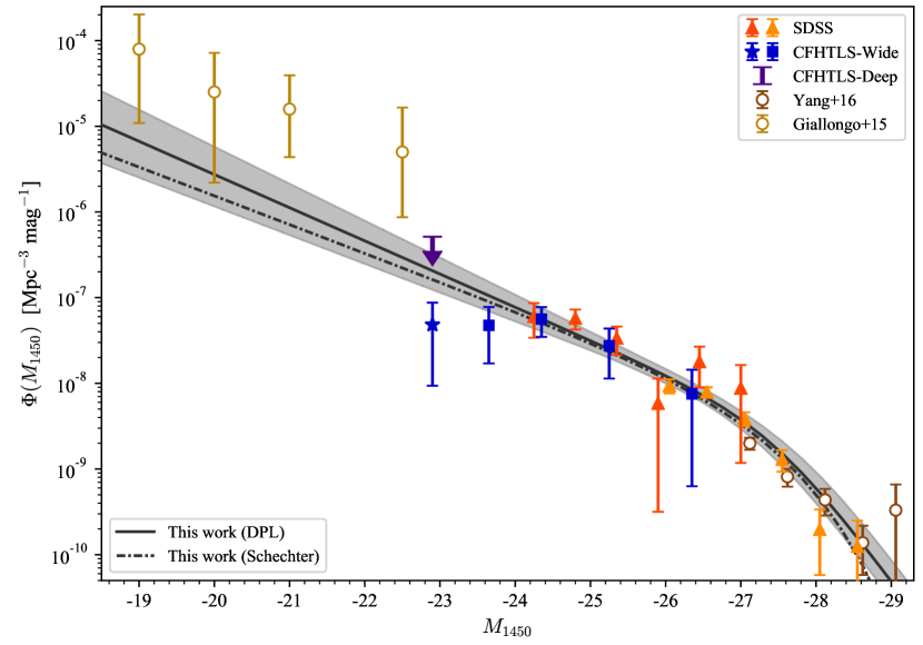
Figure 13: QLF from this work compared to Yang et al. (2016) (brown) and Giallongo et al. (2015) (dark yellow) at the bright and faint ends, respectively. The purple downward arrow marks the $3\sigma$ upper limit obtained from the CFHTLS Deep D1+DXS region. The remaining lines and points are as in Figure 12, with the addition of a gray boundary spanning the $3\sigma$ range allowed by the uncertainties in the double power law fits. Although the CFHTLS sample does not overlap the Giallongo et al. (2015) sample in luminosity, it is clear that the two QLFs do not agree at the faint end.

5.4 Parameter Estimation from Maximum Likelihood

As in Paper I, we employ maximum likelihood estimation to obtain parametric model fits to our data. Assuming an evolving luminosity function $\Phi(M,z)$ modulated by a selection function $p(M,z)$, the log likelihood function is

$$S=-2\sum\limits_{i}^{N}\ln[\Phi(M_{i},z_{i})]+2\int\int\Phi(M,z)p(M,z)\frac{dV}{dz}dMdz~{}.$$

We first fit a double power law function,

$$\Phi(M,z)=\frac{\Phi^{*}}{10^{0.4(\alpha+1)(M-M^{*})}+10^{0.4(\beta+1)(M-M^{*})}}~{},$$

where $\Phi^{*}$ is the normalization of the space density, $M^{*}$ is the break luminosity, and $\alpha$ and $\beta$ are the faint- and bright-end slopes, respectively. We consider evolution of this function within our bin of width $\Delta{z}=0.7$ by allowing the normalization to decline as a power law, $\Phi^{*}(z)=\Phi^{*}(z=6)\times 10^{k(z-6)}$, with $k=-0.47$ (Fan et al. 2001b). In Paper I we examined the evolution of both $\Phi^{*}$ and $M^{*}$ at $z\geq 4$ and found that $k=-0.47$ provides a good fit to the data out to $z\sim 5$, although there is some indication this value steepens at $z\gtrsim 6$. $M^{*}$ is also found to evolve strongly out to $z\sim 5$, although its continued evolution to higher redshift is difficult to assess and here we ignore any evolution in this parameter within our bin. We experimented with fits using $k=-0.7$ and find that the results within our redshift bin are generally insensitive to the choice of the $k$ term.

The apparent flattening of the faint-end slope based on the new measurements presented here introduces some tension with the double power law form. We thus experiment with a Schechter function parameterization of the QLF:

$$\Phi(M,z)=\frac{\ln{10}}{2.5}\Phi^{*}10^{0.4(\alpha+1)(M-M^{*})}\exp[-10^{0.4(M-M^{*})}]~{}.$$

This model requires only three parameters, similar in nature to the double power law parameters except the power-law bright-end slope is replaced by an exponential cutoff. While this functional form is commonly used to describe the galaxy luminosity function, a double power law is generally preferred by QLF measurements.

Table 2 contains the results from the maximum likelihood parameter estimation. We include the fit results from Paper I in the second column for comparison, updated to the cosmology adopted in this paper. In the third and fourth columns we present the best-fit results for the double power law and Schechter luminosity function parameterizations, respectively. Following Paper I, we have fixed the bright-end slope for the double power law to $\beta=-4$, thus the two functional forms have the same number of parameters. The log-likelihood values differ at the $<1\sigma$ level, indicating that the two forms provide an equally good fit.

Table 2: MLE fit parameters

Parameter	Paper I (DPL)	DPL	Schechter
$\log\Phi^{*}$	$-8.94^{+0.20}_{-0.24}$	$-8.97^{+0.15}_{-0.18}$	$-8.70^{+0.19}_{-0.22}$
$M_{1450}^{*}$	$-27.21^{+0.27}_{-0.33}$	$-27.47^{+0.22}_{-0.26}$	$-27.33^{+0.26}_{-0.32}$
$\alpha$	$-2.03^{+0.15}_{-0.14}$	$-1.97^{+0.09}_{-0.09}$	$-1.84^{+0.12}_{-0.11}$
$\beta$	$-4.00$	$-4.00$	-

Note. — Parameters without uncertainty ranges are fixed during the maximum likelihood fitting.

5.5 Comparison to Previous Work

We first compare our results to those from Paper I. Comparison of the best-fit double power law values in Table 2 shows that the new fits are in good agreement with the previous results, with all parameters agreeing within the $1\sigma$ ranges. The QLF models shown in Figure 12 demonstrate that the new double power law fit has almost no effect on the faint end number counts, although the Schechter form predicts number counts at lower luminosities that are a factor of $\sim 2$ lower than the double power law extrapolation.

Figure 13 places our new QLF measurement in the context of other measurements at $z\sim 5$. The bright end of the luminosity function was recently assessed by Yang et al. (2016) using a combination of SDSS and WISE colors. At $M_{1450}\leq-28$ our results are in good agreement. Our number densities are slightly higher at lower luminosities, which may be due to the efficiency of WISE selection at these redshifts. Yang et al. (2016) found a best-fit bright-end slope of $\beta=-3.6$, somewhat flatter than the fixed value of $\beta=-4$ we adopted; however, our results are rather insensitive to the value of $\beta$. They also find a somewhat fainter break luminosity of $M_{1450}^{*}=-27$, although the two results agree within the $1\sigma$ uncertainties.

At the faint end of the luminosity function we find a much lower number density than implied by the results of Giallongo et al. (2015) based on photometric redshifts of putative X-ray detections in the GOOD-S field. Where the two measurements nearly overlap our counts are lower by more than one order of magnitude. We consider the maximum possible number density consistent with our survey in two ways. First, we assess the allowed range of QLF fits by performing 1000 Monte Carlo samplings of the best-fit double power law parameters, keeping those with a log-likelihood within $1\sigma$ of the best-fit result. This range is marked by the gray shaded region. Second, we obtain a density from the single quasar in the D1 field. The $3\sigma$ upper limit for the density at $M_{1450}=-22.9$ obtained from this object is denoted by the purple error bar with a downward arrow. As argued in §3.5, we expect the selection in the D1 region to be highly complete and thus this upper limit provides a strong constraint on the faint number counts. Recently, Parsa et al. (2017) performed a re-analysis of the Giallongo et al. (2015) sample, and find a number density at $z\sim 5$ about a factor of $\sim 3$ lower, in much better agreement with our results.

Repeating the procedure of Giallongo et al. (2015), we derive an ionizing emissivity at $z\sim 5$ that is almost an order of magnitude lower: $\epsilon_{912}^{24}=0.8$ as opposed to $\epsilon_{912}^{24}=5.9$ in Giallongo et al. (2015) (compare to $\epsilon_{912}^{24}=1.3$ in Parsa et al. 2017). Based on these results it is highly unlikely that faint AGN make a significant contribution to hydrogen reionization (see also D’Aloisio et al. 2017; Khaire 2017; Ricci et al. 2017), unless our survey is highly incomplete or the extrapolation to fainter sources does not follow the QLF we have derived.

Finally, we compare our results to measurements of the X-ray QLF from wide-area surveys as given in Georgakakis et al. (2015, see also ). Assuming typical values for the X-ray/optical flux ratio, Georgakakis et al. (2015) found that the QLF we obtained in Paper I is nearly an order of magnitude below the X-ray counts at a similar luminosity. Our new results favor an even flatter slope at the faint end. This suggests that a significant fraction of black hole growth at low luminosities may be highly obscured (see also Trakhtenbrot et al. 2016).

5.6 Conclusions

We present a sample of 104 candidate $z\sim 5$ quasars drawn from the CFHTLS Wide survey. Spectroscopic confirmations for 37 quasars were obtained using Gemini-GMOS, MMT Red Channel, and LBT-MODS. The luminosity function derived from these quasars is in good agreement with our previous measurements using SDSS Stripe 82 (Paper I). The faintest quasars in the sample reach $M_{1450}=-22.9$, with the full luminosity function extending over a range of 6 mag.

Parametric fits to the luminosity function obtained using a maximum likelihood method show that the break in the luminosity function is at $M_{1450}\approx-27$, in agreement with the evolutionary model presented in Paper I that includes a steady increase in the break luminosity with increasing redshift. Although the best-fit faint-end slope is somewhat steep ($\alpha\approx-2$), the data in the lowest luminosity bins are below the best-fit QLF, suggesting the faint number counts may be even fewer. In addition to the traditional double power-law form for the QLF, a Schechter function is found to provide an equally good fit to the overall data, and provides a marginally better fit to the faint number counts.

These results do not support a scenario in which faint AGN provide a significant contribution to the hydrogen-ionizing radiative background at $z\sim 5$. Integrating the best-fit QLF to $M_{1450}=-18$ results in quasars producing only a few per cent of the ionizing photons required to maintain hydrogen ionization. This is contrary to recent claims of a significant faint AGN population based on photometric redshifts of galaxies associated with X-ray emission (Giallongo et al. 2015, although see Parsa et al. 2017).

We consider potential sources of incompleteness in our survey, focusing on the effect of Ly$\alpha$ emission as this has a significant impact on optical color selection. We find marginal evidence for weaker Ly$\alpha$ emission in our faintest quasars compared to a luminosity-matched sample at $z\sim 3$ from BOSS. If Ly$\alpha$ is systematically weaker at high redshift, our selection efficiency may be overestimated. However, this is unlikely to substantially alter the conclusion that quasars are insufficient in number to drive hydrogen reionization. Future studies that can efficiently select high-$z$ quasars using methods independent of the Ly$\alpha$ flux – e.g., color selection in infrared bands (Wang et al. 2016; Yang et al. 2016), or variability selection (Peters et al. 2015; AlSayyad 2016) – will address this issue and form a more complete picture of the faint quasar population near the epoch of reionization.

6 Acknowledgments

I. D. McGreer and X. Fan acknowledge the support from the U.S. NSF grant AST 15-15115. L.J. acknowledge support from the National Key R&D Program of China (2016YFA0400703). The work presented here is based in part on observations obtained at the Gemini Observatory, which is operated by the Association of Universities for Research in Astronomy, Inc., under a cooperative agreement with the NSF on behalf of the Gemini partnership: the National Science Foundation (United States), the National Research Council (Canada), CONICYT (Chile), the Australian Research Council (Australia), Ministério da Ciência, Tecnologia e Inovação (Brazil) and Ministerio de Ciencia, Tecnología e Innovación Productiva (Argentina). Gemini data were processed using the Gemini IRAF package and gemini_python. Additional observations were obtained at the MMT Observatory, a joint facility of the Smithsonian Institution and the University of Arizona. Also based on observations obtained with MegaPrime/MegaCam, a joint project of CFHT and CEA/DAPNIA, at the Canada-France-Hawaii Telescope (CFHT) which is operated by the National Research Council (NRC) of Canada, the Institut National des Science de l’Univers of the Centre National de la Recherche Scientifique (CNRS) of France, and the University of Hawaii. This work is based in part on data products produced at the Canadian Astronomy Data Centre as part of the Canada-France-Hawaii Telescope Legacy Survey, a collaborative project of NRC and CNRS.

This work made use of the following open source software: IPython (Perez & Granger 2007), matplotlib (Hunter 2007), NumPy (van der Walt et al. 2011), SciPy (Oliphant 2007), Astropy (The Astropy Collaboration et al. 2013), and astroML (VanderPlas et al. 2012). This research has made use of NASA’s Astrophysics Data System.

Facilities: Gemini:Gillett (GMOS), LBT (MODS1), MMT (Red Channel spectrograph), CFHT (MegaCam)

7 Appendix

7.1 Color selection and weak-lined quasars

The efficiency of our selection method relies on the colors of $z\sim 5$ quasars becoming redder in $r-i$ and bluer in $i-z$ than stars in a similar region of color space (Fig. 4). This is due to a combination of the attenuation in bands blueward of the $i$-band from the strong IGM absorption, and the generally prominent Ly$\alpha$ emission from the quasar. Because Ly$\alpha$ is within the $i$-band at these redshifts, stronger Ly$\alpha$ emission increases the contrast between quasars and stars and hence the selection efficiency. We noted this effect in Paper I (Fig. 13 and surrounding discussion), where we showed that our color selection is expected to be relatively more sensitive to fainter quasars, which tend to have stronger Ly$\alpha$ emission associated with the Baldwin Effect (Baldwin 1977).

A potential concern is the fraction of quasars with weak emission lines. Using our color simulations, we find that removing the emission lines completely (the most extreme case of a weak-lined quasar) indeed shifts the $riz$ colors towards the boundary of our color box. In Paper I, we noted that the fraction of weak-lined quasars, defined as EW₀(Ly$\alpha$+N V) $<15$Å by Diamond-Stanic et al. (2009), is $\sim 6\%$ for SDSS quasars at $z\gtrsim 4$ where the selection efficiency of weak-lined objects is relatively high (see their Fig. 5). We thus expect a minimal correction to the luminosity function from this class of objects unless the weak-lined fraction evolves dramatically from $z\sim 4$ to $z\sim 5$, or if it is much higher for the low luminosity objects in our sample compared to the more luminous SDSS quasars in Diamond-Stanic et al. (2009).

Weak emission lines may arise due to intrinsic properties of quasars, e.g., a softer ionizing continuum or shielding gas (Wu et al. 2012; Plotkin et al. 2015; Shemmer & Lieber 2015). While it is not known whether or not these properties evolve with redshift, in general, the spectral properties of quasars appear to show little redshift evolution (e.g., Kuhn et al. 2001; Yip et al. 2004; Jiang et al. 2006). On the other hand, the Ly$\alpha$ emission may be affected by strong neutral absorbers near the quasar redshift. While the line-of-sight proximity effect is generally suppressed in lower redshift, high-luminosity quasars (Bajtlik et al. 1988; Hennawi et al. 2006, although see Dall’Aglio et al. 2008) likely due to the strong ionizing radiation from the quasar, in our sample of faint, $z\sim 5$ quasars the incidence of self-shielded absorption systems may be greater (see related discussions in Hennawi & Prochaska 2007; Bolton & Haehnelt 2013), the mean UV background emission is weaker (Calverley et al. 2011), and the expected proximity zone sizes are smaller (e.g., Eilers et al. 2017), all of which may lead to greater Ly$\alpha$ absorption. Additionally, if the Ly$\alpha$ emission line in high-$z$ quasars is systematically blueshifted it may be suppressed by strong IGM absorption from dense gas, even if it is highly ionized (cf. Keating et al. 2015, for a discussion of red damping wings from highly ionized environs). Ly$\alpha$ blueshifts are correlated with C IV blueshifts (Kramer & Haiman 2009), which are commonly found in luminous quasars (Mortlock et al. 2011; Richards et al. 2011; Bosman & Becker 2015).

In the most extreme case, if low-luminosity $z\sim 5$ quasars tend to have extremely weak Ly$\alpha$ emission, our selection efficiency would be greatly reduced. In this Appendix we examine in detail the dependence of our color selection efficiency on the Ly$\alpha$ emission properties. Our quasar models are calibrated using SDSS/BOSS quasars at $2<z<3.5$; any differences between the spectra of $z\sim 3$ and $z\sim 5$ quasars will impact our luminosity function calculation.

7.2 Quasar samples with Ly$\alpha$ coverage

Our comparison sample is constructed from $z\sim 3$ quasars from the SDSS DR7QSO catalog (Schneider et al. 2010) and the BOSS DR9QSO catalog (Paris et al. 2012). For the DR7QSO quasars we adopt the redshifts provided by Hewett & Wild (2010), and for DR9QSO we use the PCA redshifts (Z_PCA, Paris et al. 2012). We then select quasars with $2.4<z<3.5$, providing coverage of the Ly$\alpha$ region. For the BOSS quasars we further restrict the sample to quasars in Stripe 82, which are predominantly selected by variability (Palanque-Delabrouille et al. 2011), reducing any color selection bias that would disfavor objects with weak lines. The BOSS sample includes $\sim 900$ quasars that were observed in SDSS I/II and present in the DR7QSO sample. The BOSS and SDSS spectra are independent and we choose to retain these objects in both samples. The final $z\sim 3$ comparison set consists of $\sim$5700 BOSS and $\sim 10000$ SDSS quasars and spans $-28\lesssim M_{1450}\lesssim-23$.

We also draw on the DR7QSO and DR9QSO catalogs to select luminous $z\sim 5$ quasars, obtaining $\sim 400$ ($\sim 150$) quasars from SDSS (BOSS) in the range $4.5<z<5.5$. Finally, we include fainter quasars from our own survey, with $\sim 75$ MMT spectra and 5 Gemini spectra of $z\sim 5$ quasars.

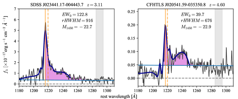
Figure 14: Examples of non-parametric estimation of line features. The left panel displays the spectrum of a $z\sim 3$ quasar from BOSS with a gray line, and the right panel a Gemini spectrum of a $z\sim 5$ quasar at a similar luminosity. The light blue line represents the power-law continuum fit as described in the text; the gray shaded region is the bluest spectral window used for continuum fitting. The dark blue line traces the smoothed spline model fit to the spectrum. The total EW of the Ly$\alpha$+N V region is obtained by direct integration above the continuum fit, as represented by the purple shaded region. The Ly$\alpha$ red HWHM is obtained from the peak wavelength (solid orange line) and the wavelength at which the smoothed profile drops to 60% of the peak value (dashed orange line, scaled to HWHM position for a Gaussian profile).

7.3 Method

The Ly$\alpha$ emission region of high-redshift quasars consists of a complex set of emission and absorption features. We initially attempted to fully model the Ly$\alpha$ region using a series of Gaussians for the Ly$\alpha$ $\lambda$1216, N V $\lambda$1240, and Si II $\lambda$1261 emission features, including both a broad and narrow component for Ly$\alpha$. However, we found that reliable decomposition of this region into multiple Gaussians was extremely difficult due to the varied shapes of the line profiles, strong absorption features (from both intrinsic Ly$\alpha$ and BAL-type absorption), Ly$\alpha$ forest absorption, and the relatively low $S/N$ of the spectra.

We thus adopted non-parametric approaches to characterize the Ly$\alpha$ emission. First, we quantify the total EW of the emission region (including Ly$\alpha$, N V, and Si II) using the method of Diamond-Stanic et al. (2009). Briefly, a power-law continuum is fit to a set of spectral windows relatively uncontaminated by emission lines. After dividing the power-law continuum, the total EW is obtained by summing the residual (positive) emission; as in Diamond-Stanic et al. (2009) we refer to this quantity as EW₀(Ly$\alpha$+N V). One difference with the method of Diamond-Stanic et al. (2009) is that we sum over the wavelength range $1216<\lambda<1290$ instead of $1160<\lambda<1290$. Truncating the blue edge of the region at Ly$\alpha$ provides a more reasonable comparison between $z\sim 3$ and $z\sim 5$ spectra, as otherwise the results would be affected by the increased IGM absorption blueward of Ly$\alpha$ between those redshifts.

Next, we roughly quantify the width of the core the Ly$\alpha$ line, which is typically dominated by the narrow component. For this we use the half-width at half-maximum of the profile redward of line center (rHWHM). Using the red side avoids regions affected by Ly$\alpha$ forest absorption. However, the red side is affected by blending from N V emission and also strong absorption features that appear in many spectra (usually N V BAL-type absorption). To address these issues, we fit a heavily smoothed spline model to the line profile. The spline models were derived by iteratively fitting splines of increasing flexibility while masking pixels significantly below the low-order fits to remove absorption features.

After obtaining the spline models, we calculate the half-width at 65% of the peak, instead of 50%, as we found this value to be less affected by contamination from the neighboring lines while still providing a reasonable estimate of the line width. The calculated value is then scaled appropriately for a Gaussian to the half-power width in order to obtain the rHWHM estimate. Examples of Ly$\alpha$ fitting for a BOSS quasar at $z=3.1$ and a Gemini spectrum of a faint CFHTLS quasar at $z=4.6$ are presented in Figure 14.

We stress that the both quantities (EW₀ and rHWHM) are obtained using exactly the same procedure on the spectra from the different quasar samples.

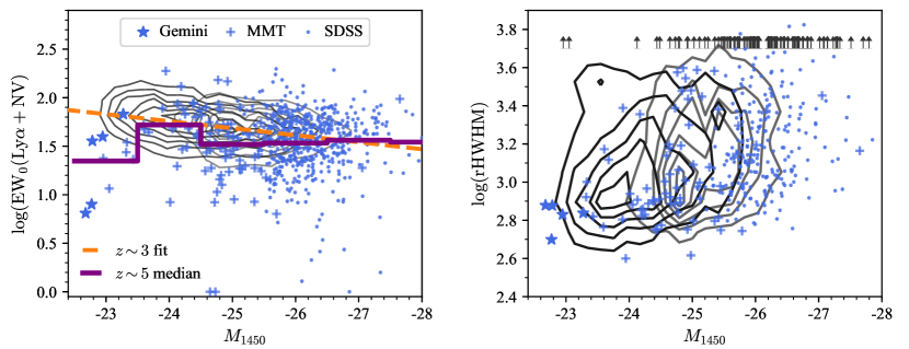
Figure 15: Left: Distribution of rest-frame EW of the combined Ly$\alpha$+N V emission lines for various high-redshift quasar samples. The black (gray) contours represent the distribution of EWs measured from luminous quasars at $2.4<z<3.5$ from DR7QSO (DR9QSO). The $z\sim 5$ data are represented with circles. A running median of the $z\sim 5$ points in bins of width $\Delta{m}=1$ is marked with the solid brown line. Right: rHWHM measurements. Lines and symbols are same as the left panel. Objects with rHWHM $>5000~{}{\rm km}~{}{\rm s}^{-1}$ are displayed as upward pointing arrows at $\log({\rm rHWHM})=3.7$; these cases are usually due to contamination from broad Ly$\alpha$ or N V.

7.4 Results

Figure 15 displays measurements of EW₀(Ly$\alpha$+N V) from our quasar samples. The grayscale contours represent the distribution of EWs measured from $z\sim 3$ SDSS/BOSS quasars, and show a clear trend of increasing EW with decreasing luminosity (the Baldwin Effect). This trend can be recovered with a linear fit to the data, represented by the dashed orange line which is $\log(\mathrm{EW}_{0})=1.7+0.07(M_{1450}+25)$. The scatter points represent the measurements from $z\sim 5$ quasars. At high luminosities they overlap the $z\sim 3$ data, but at the lowest luminosities there appears to be a dearth of high-EW quasars as expected from the extrapolation of the $z\sim 3$ sample. The solid purple line marks the median EW in bins of width 1 mag in luminosity. For $z\sim 5$ quasars with a luminosity $M_{1450}\approx-23$ the median is $\langle$EW₀(Ly$\alpha$+N V)$\rangle=1.3$, which is $\sim 0.5$ dex lower than the relation for the $z\sim 3$ quasars. That is, if the $z\sim 3$ population were shifted to $z\sim 5$, we should expect a median EW $\approx 70$, but the median of the observed $z\sim 5$ quasars is $\approx 24$. Only 1/10 of the $M_{1450}\approx-23$ quasars has EW $>40$.

Another check on whether there is evolution in the intrinsic emission properties of quasars between $z\sim 3$ and $z\sim 5$ is to examine the profile width of the Ly$\alpha$ emission line. The right panel of Figure 15 shows that the measurements of rHWHM for the two redshift ranges are broadly consistent, although this is a noisy measurement. We were motivated to perform this check after noticing the narrowness of the lines presented by the low-luminosity objects (cf. Matsuoka et al. 2017); however, as can be seen in Figure 15 the $z\sim 5$ objects are not outliers from the general trend with luminosity observed at $z\sim 3$.

7.5 Implications for completeness

We now examine the effect of varying the Ly$\alpha$ emission in our quasar completness models. Figure 16 compares the selection efficiency along two parameters: Ly$\alpha$ EW and UV continuum slope. We use a grid of simulated quasars at $z\sim 5$ modeled as a simple power-law continuum with index $\alpha_{\nu}$ and a single Gaussian emission line at 1216Å. The grid includes $\alpha_{\nu}=(-1.5,-1.0,-0.6,-0.4,-0.2,0.0)$ and $\mathrm{EW}_{0}({\rm Ly}\alpha[\AA])=(0,15,30,60,120)$. We then run the simulation with this simplistic model while allowing for random sampling of the Ly$\alpha$ forest transmission and the random scatter of the photometry . The left panel shows the mean selection function at $\alpha_{\nu}=-0.4$ (a typical value for quasars, Vanden Berk et al. 2001) as the Ly$\alpha$ EW is varied. The selection function prefers quasars with high EW. Thus it is interesting that our observed sample presents a dearth of high EW quasars at $z\sim 5$ compared to quasars at a similar (low) luminosity at $z\sim 3$.

The right panel shows the mean selection function at $\mathrm{EW}_{0}({\rm Ly}\alpha)=30$Å, roughly matching our measurements of $z\sim 5$ quasars. The dependence on spectral index is less strong, although bluer quasars tend to be selected less efficiently at low redshift and more efficiently at high redshift.

The efficiencies for both the weak (solid lines) and strict (dashed) color criteria are presented in Figure 16. We have a substantial amount of spectroscopic coverage for candidates selected by the strict criteria, and for the faint quasar sample the coverage is complete. We also select candidates after applying the weak color criteria but adding a likelihood cut for both the bright and faint candidate samples. Thus our true completeness lies somewhere between the dashed and solid curves in Figure 16.

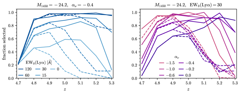
Figure 16: Left: Selection function dependence on Ly$\alpha$ EW for $\alpha_{\nu}=-0.4$. The line shading represents increasing Ly$\alpha$ EW. Solid (dashed) lines are for the weak (strict) color selection criteria. At fixed luminosity ($M_{1450}=-24.2$) the selection efficiency for the weak cuts drops by a factor of $\sim 2$ as the Ly$\alpha$ flux goes to zero. The strict cuts largely exclude $z\gtrsim 5$ quasars with modest Ly$\alpha$ EW. Right: Selection function at fixed Ly$\alpha$ EW for different UV spectral slopes. In general the dependence on UV slope is much weaker.

Although our selection function clearly depends on the Ly$\alpha$ EW, a $z=4.9$ quasar with $\mathrm{EW}_{0}({\rm Ly}\alpha)=15$Å has a $\sim 70$% chance of being selected by either the weak or strict color criteria. This is the boundary used to define weak-lined quasars by (Diamond-Stanic et al. 2009). A quasar with no Ly$\alpha$ emission has a $\sim 50$% ($\sim 35$%) probability of being selected by the weak (strict) color criteria. Unless weak-lined quasars completely dominate the population at $z\sim 5$, we are likely overestimating our completeness at the lowest luminosities by at most a factor of $\sim$2–3. The median of our observed sample at $\sim 24$Å, suggesting that we are not overestimating our completeness by such a large factor. Future surveys less reliant on optical colors will be better suited to address this outstanding issue.

7.6 Additional quasars

We obtained spectroscopic observations of a number of objects not included in our final candidate sample. These can be broken into three groups. First, there are 10 $z\sim 5$ quasars identified in the CFHTLS using early implementations of our color and likelihood selection methods, but excluded from the final sample. Second, we obtained spectra for five candidates from our Stripe 82 sample in Paper I (see Table 3 in that paper) that previously lacked identifications. Finally, during poor observing conditions we observed bright backup targets from the SDSS DR7 imaging. The full list of additional quasars is given in Table 3 and the MMT spectra can be viewed in Figure 17.

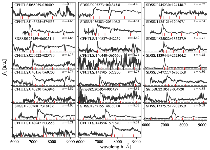
Figure 17: MMT spectra of quasars not included in final sample, corresponding entries are in Table 3. Names starting with “SDSS” are from SDSS DR7, “Stripe82” from SDSS Stripe 82, and “CFHTLS” from CFHTLS Wide.

Table 3: Quasars with spectroscopy not included in final candidate sample

R.A. (J2000)	Decl. (J2000)	$z$	Source	R.A. (J2000)	Decl. (J2000)	$z$	Source
01:25:45.49	+06:02:51.1	4.65	DR7	14:09:42.30	+53:35:58.2	5.21	CFHT
07:45:23.90	+12:41:48.7	4.57	DR7	14:19:56.59	+57:18:40.4	5.31	CFHT
08:25:02.42	+13:52:27.9	4.71	DR7	14:31:56.36	+56:02:00.8	4.75	CFHT
08:50:39.71	-03:04:09.6	4.18	CFHT	14:36:25.45	+57:45:55.8	4.58	CFHT
09:05:27.43	+04:43:43.8	4.40	DR7	14:37:05.17	+52:28:00.7	4.78	CFHT
09:47:22.87	+69:36:15.8	4.80	DR7	14:38:30.83	+56:39:46.4	4.82	CFHT
10:36:38.93	+20:54:06.2	4.61	DR7	17:57:15.95	+48:36:01.8	5.03	DR7
11:25:12.21	+12:06:07.1	4.64	DR7	20:37:53.64	+00:05:49.4	-	S82
12:00:26.28	+23:18:18.6	4.90	DR7	20:59:54.11	-00:54:27.7	4.82	S82
13:32:57.45	+22:08:35.9	5.09	DR7	21:00:41.31	-00:52:03.4	-	S82
13:39:44.03	+25:23:04.2	4.75	DR7	21:05:17.97	-00:49:20.3	4.85	S82
14:04:40.29	+56:56:50.7	4.74	CFHT	21:47:30.25	+00:12:37.5	-	S82
14:08:37.46	+54:22:59.7	4.69	CFHT	22:05:22.15	+02:57:30.0	4.73	CFHT

Note. — The final column lists the imaging source from which the object was selected: DR7 - SDSS DR7, S82 - SDSS Stripe 82, CFHT - CFHTLS Wide. Three non-quasars from the Stripe 82 complete sample given in Paper I are listed with dashes for the redshift entry.

Table 4: Complete sample of quasar candidates with $i_{\rm AB}<23.2$ selected from the CFHTLS Wide fields W1, W2, and W3, and with partial spectroscopic coverage from Gemini-N, MMT, and LBT.

R.A.	Decl.	$g_{\rm AB}$	$r_{\rm AB}$	$i_{\rm AB}$	$z_{\rm AB}$	${\rm\tt PQSO}$	${\rm\tt PQSOMIDZ}$	$M_{1450}$	$z$	Tel.
02:01:00.41	-05:52:30.2	26.04	23.30	21.67	21.72	1.0	1.0
02:01:02.44	-05:04:08.6	25.59	22.94	21.17	20.88	1.0	0.00
02:01:53.71	-05:04:27.2	$>$26.6	24.57	22.67	22.21	1.0	0.0
02:01:58.30	-08:00:48.9	25.34	23.28	21.53	21.63	1.0	1.0
02:02:15.60	-08:01:21.3	27.40	25.32	22.84	22.46	1.0	0.0
02:03:13.48	-05:21:37.9	$>$26.6	24.92	22.73	23.16	1.0	1.0
02:03:19.34	-07:55:08.2	26.61	24.75	22.99	22.74	0.99	0.95
02:03:35.87	-05:03:11.1	$>$26.6	24.15	22.82	22.62	1.0	1.0
02:04:03.11	-06:23:58.2	26.09	23.73	21.98	21.83	1.0	1.0
02:05:33.92	-07:08:49.1	26.61	24.78	23.07	22.59	0.00	0.0
02:05:41.59	-03:53:50.8	26.45	24.64	23.16	23.10	0.97	0.06	-22.9	4.60	Gem
02:05:54.37	-06:26:24.0	27.66	23.81	22.25	22.01	1.0	0.0
02:09:08.47	-05:01:07.4	28.67	24.15	22.75	22.41	1.0	1.0
02:09:42.92	-09:27:14.2	26.86	24.57	22.83	23.17	1.0	0.77
02:10:54.68	-03:42:55.0	$>$26.1	24.64	22.68	22.23	1.0	0.0
02:11:01.49	-03:56:29.0	26.91	24.77	22.96	22.46	0.18	0.00
02:12:47.67	-05:00:02.8	25.20	23.16	21.79	21.70	1.0	0.0
02:12:57.80	-08:09:36.8	26.35	24.37	22.65	22.20	0.0	0.0
02:13:05.72	-10:05:47.9	26.43	24.43	23.04	22.81	0.99	0.01
02:14:46.81	-09:04:35.2	26.48	24.60	23.09	22.85	0.71	0.00
02:14:48.81	-08:07:46.7	$>$26.9	25.04	23.18	22.72	0.97	0.00
02:15:07.29	-05:18:49.2	26.29	24.28	22.82	22.72	1.0	0.01
02:15:07.82	-08:36:59.2	25.96	23.97	22.64	22.63	1.0	0.0
02:15:19.38	-09:50:18.7	$>$26.2	24.58	22.82	23.00	1.0	0.99
02:15:23.27	-05:29:45.8	28.05	22.69	20.85	20.64	1.0	1.0	-25.7	5.13	MMT
02:16:09.59	-08:41:41.1	$>$26.8	24.52	22.41	22.00	1.0	0.0
02:17:07.49	-09:54:45.2	27.05	23.97	22.34	22.15	1.0	1.0
02:18:00.49	-04:47:18.5	26.41	24.52	23.16	23.14	1.0	0.00
02:19:54.18	-08:29:48.8	$>$26.8	24.57	22.45	22.21	1.0	0.99
02:21:12.32	-03:42:31.6	25.82	23.59	21.42	21.48	1.0	1.0	-24.9	5.02	MMT
02:21:12.61	-03:42:52.2	24.10	21.22	19.38	19.52	0.0	0.0	-27.1	5.02	MMT
02:23:15.88	-05:27:30.0	26.49	23.03	21.58	21.28	1.0	1.0
02:24:45.08	-08:42:28.7	25.26	22.62	20.98	20.98	1.0	1.0
02:25:15.76	-06:31:15.1	$>$26.3	24.46	22.44	22.04	1.0	0.0
02:26:04.73	-09:18:18.7	27.53	22.54	20.82	20.53	1.0	1.0
02:26:42.39	-08:38:00.4	26.19	23.86	22.07	22.13	1.0	1.0
02:27:35.87	-08:08:40.9	26.56	24.63	23.15	22.96	1.0	0.16	-	-	Gem
02:27:40.24	-07:43:33.8	26.64	23.32	21.73	21.34	1.0	0.0
02:30:59.02	-06:39:55.7	27.47	24.46	22.99	22.74	1.0	0.32
02:31:19.76	-08:10:07.1	26.03	24.17	22.67	22.42	1.0	0.0
02:31:37.64	-07:28:54.4	$>$26.6	21.35	19.41	19.15	0.0	0.0	-27.7	5.37	MMT
02:32:45.46	-06:02:03.1	26.32	23.47	21.87	21.80	1.0	1.0
13:57:47.34	+53:05:42.5	28.27	23.32	21.29	20.85	1.0	0.0	-25.6	5.32	MMT
13:58:55.97	+51:43:17.0	25.74	22.11	20.33	20.34	0.0	0.0	-26.0	4.97	MMT
14:01:46.97	+56:41:44.7	25.87	23.47	21.49	21.68	1.0	0.0	-24.8	4.98	MMT
14:01:49.96	+51:43:10.3	28.28	24.54	22.85	23.05	1.0	0.99	-23.0	4.20	MMT
14:02:41.71	+52:39:08.2	26.65	24.63	23.11	23.05	1.0	0.36	-	-	MMT
14:05:17.99	+54:00:03.2	$>$26.1	25.09	23.10	22.61	1.0	0.0
14:06:02.15	+56:07:19.1	28.77	24.47	23.06	22.98	1.0	0.66	-23.0	4.62	MMT
14:07:10.12	+51:24:15.1	27.00	24.56	23.08	22.63	0.42	0.31
14:07:29.55	+53:45:55.7	26.46	24.15	22.77	22.37	0.36	0.36
14:08:22.92	+53:00:20.9	25.11	22.75	20.99	21.16	1.0	1.0	-25.5	5.07	MMT
14:08:50.27	+54:41:43.5	27.20	24.59	23.00	22.62	1.0	0.94
14:12:45.95	+54:46:36.9	26.08	24.17	22.61	22.33	1.0	0.39
14:13:22.22	+57:45:53.5	25.92	23.04	21.43	21.40	1.0	1.0	-24.7	4.79	MMT
14:13:26.58	+57:47:06.5	27.44	23.61	21.73	21.80	1.0	1.0	-24.5	4.94	MMT
14:14:04.36	+51:15:35.8	$>$26.5	23.56	21.86	21.45	1.0	0.0	-24.8	5.24	MMT
14:14:31.57	+57:32:34.1	27.61	23.37	21.73	21.51	1.0	1.0	-24.8	5.16	MMT
14:14:46.82	+54:46:31.8	27.31	25.08	23.02	23.34	1.0	0.95	-23.9	5.42	MMT
14:18:42.69	+54:41:31.2	26.37	23.15	21.74	21.44	1.0	1.0	-24.5	4.92	MMT
14:18:45.92	+54:47:20.7	29.06	24.50	23.18	22.95	0.99	0.62
14:18:58.99	+54:05:12.2	28.08	24.75	23.11	22.63	0.73	0.16
14:19:29.54	+51:23:56.1	26.74	24.56	23.05	22.74	0.34	0.21
14:19:56.49	+55:53:16.2	$>$26.4	25.69	23.17	22.95	1.0	0.00	-	5.0?	MMT
14:24:08.15	+51:42:23.8	27.03	24.59	22.78	22.29	1.0	0.0
14:25:19.30	+51:38:15.6	28.35	25.04	23.15	23.29	1.0	0.98	-23.0	4.84	MMT
14:26:17.28	+51:55:59.4	26.46	23.79	22.22	21.91	1.0	0.99	-23.9	4.69	MMT
14:26:34.87	+54:36:22.7	23.95	21.54	19.79	20.01	0.0	0.0	-26.4	4.76	MMT
14:28:53.84	+56:46:02.1	26.07	23.76	21.99	21.84	1.0	1.0	-24.1	4.73	MMT
14:36:49.39	+54:15:12.1	26.56	24.66	23.15	23.06	0.99	0.31
14:37:21.78	+54:28:19.6	24.66	22.42	20.90	20.78	1.0	1.0
14:37:56.54	+51:51:15.1	$>$26.6	24.25	22.37	22.21	1.0	0.98	-24.2	5.17	MMT
14:38:04.05	+57:36:46.3	27.55	24.23	22.52	22.68	1.0	1.0	-23.6	4.84	MMT
14:38:06.51	+54:46:03.3	25.83	23.95	22.21	21.77	1.0	0.0
14:39:15.95	+53:06:22.9	$>$26.7	24.61	22.67	22.37	1.0	0.88	-23.4	4.77	MMT
14:39:44.87	+56:26:26.5	27.01	24.43	22.78	22.63	1.0	0.99	-23.3	4.70	MMT
21:59:55.17	+01:15:12.9	29.20	24.64	22.96	22.70	1.0	0.38
22:02:33.20	+01:31:20.3	28.16	23.95	22.09	22.02	1.0	0.14	-24.6	5.23	LBT
22:02:39.31	+01:03:45.2	26.64	24.80	23.12	22.74	0.03	0.01
22:09:12.11	+01:32:46.2	26.58	24.36	22.62	22.21	1.0	0.00
22:11:41.01	+00:11:18.9	$>$26.7	23.99	21.91	21.73	1.0	1.0	-24.8	5.23	MMT
22:12:13.43	-00:04:19.4	26.91	24.58	23.07	23.18	1.0	0.33
22:12:51.49	-00:42:30.7	23.87	21.82	19.80	19.95	0.0	0.0	-27.4	5.42	Sloan
22:13:05.26	+00:34:07.8	27.45	24.46	22.76	22.26	0.92	0.0	-24.0	5.31	MMT
22:13:09.67	-00:24:28.1	27.37	24.47	22.52	22.59	1.0	1.0	-23.6	4.80	MMT
22:14:43.52	+00:47:33.4	25.64	23.67	22.16	22.18	1.0	1.0
22:15:20.22	-00:09:08.4	$>$26.2	24.18	22.14	21.83	1.0	0.05	-24.6	5.28	MMT
22:16:21.85	+01:38:14.6	$>$26.4	24.58	22.75	22.46	1.0	0.99	-23.4	4.93	LBT
22:16:44.02	+00:13:48.1	25.07	22.03	20.45	20.40	1.0	0.0	-25.9	5.01	Sloan
22:16:51.92	+00:28:09.4	26.75	24.99	23.05	22.60	0.56	0.0
22:19:41.90	+00:12:56.1	25.24	22.81	21.48	21.52	1.0	0.0	-24.5	4.30	MMT
22:19:56.70	-00:52:40.5	27.11	24.34	22.80	22.41	0.11	0.11
22:19:56.70	+01:04:29.0	26.82	24.70	23.04	22.64	0.11	0.07
22:20:25.29	+00:19:30.5	26.90	24.86	23.15	22.68	0.00	0.0
22:20:54.77	+01:25:53.4	$>$26.3	24.78	22.91	22.47	1.0	0.02	-	-	MMT
22:21:13.74	-00:45:01.2	28.89	24.65	23.02	22.52	0.58	0.32
22:22:16.02	-00:04:05.6	29.58	23.69	21.88	21.84	1.0	1.0	-24.4	4.95	MMT

Note. — Magnitudes are on the AB system (Oke & Gunn 1983) and have been corrected for Galactic extinction. Lower limits on magnitudes are the 50% completeness limits for the associated CFHTLS pointing from Gwyn (2012). Blank entries indicate lack of spectroscopic coverage and dashes are used for spectroscopic non-quasars.

Table 5: Complete sample of quasar candidates with $23.2<i_{\rm AB}<23.7$ selected from the CFHTLS Wide field W1 and with partial spectroscopic coverage from Gemini-N. Format is as in Table 4.

R.A.	Decl.	$g_{\rm AB}$	$r_{\rm AB}$	$i_{\rm AB}$	$z_{\rm AB}$	${\rm\tt PQSO}$	${\rm\tt PQSOMIDZ}$	$M_{1450}$	$z$
02:05:46.63	-09:55:23.7	$>$26.6	26.18	23.55	23.37	1.0	0.10	-23.3	5.37
02:06:18.65	-04:08:55.5	28.46	24.94	23.32	23.10	1.0	0.87	-22.8	4.87
02:10:56.76	-05:58:40.4	26.87	24.93	23.42	23.11	0.05	0.00
02:21:13.96	-10:09:33.9	27.10	26.18	23.69	23.20	0.0	0.0	-	-
02:26:29.06	-04:37:04.5	$>$26.5	24.87	23.41	23.19	1.0	0.97	-22.7	4.85
02:31:15.46	-08:19:07.1	27.55	25.29	23.33	23.26	1.0	0.85	-22.8	4.52
02:33:49.79	-06:45:51.5	$>$26.5	25.25	23.52	23.05	0.54	0.01	-	-

References

- Agarwal et al. (2014) Agarwal, B., Dalla Vecchia, C., Johnson, J. L., Khochfar, S., & Paardekooper, J.-P. 2014, MNRAS, 443, 648
- Ahn et al. (2012) Ahn, C. P., Alexandroff, R., Allende Prieto, C., et al. 2012, ApJS, 203, 21
- AlSayyad (2016) AlSayyad, Y. 2016, PhD thesis, University of Washington
- Bajtlik et al. (1988) Bajtlik, S., Duncan, R. C., & Ostriker, J. P. 1988, ApJ, 327, 570
- Baldwin (1977) Baldwin, J. A. 1977, ApJ, 214, 679
- Bañados et al. (2016) Bañados, E., Venemans, B. P., Decarli, R., et al. 2016, ApJS, 227, 11
- Becker et al. (2014) Becker, G. D., Bolton, J. S., Madau, P., et al. 2014, eprint arXiv:1407.4850
- Begelman & Volonteri (2016) Begelman, M. C., & Volonteri, M. 2016, eprint arXiv:1609.07137, 1609.07137
- Bolton & Haehnelt (2013) Bolton, J. S., & Haehnelt, M. G. 2013, MNRAS, 429, 1695
- Boroson & Green (1992) Boroson, T. A., & Green, R. F. 1992, ApJS, 80, 109
- Bosman & Becker (2015) Bosman, S. E. I., & Becker, G. D. 2015, MNRAS, 452, 1105
- Bovy et al. (2011) Bovy, J., Hennawi, J. F., Hogg, D. W., et al. 2011, ApJ, 729, 141
- Calverley et al. (2011) Calverley, A. P., Becker, G. D., Haehnelt, M. G., & Bolton, J. S. 2011, MNRAS, 412, 2543
- Dall’Aglio et al. (2008) Dall’Aglio, A., Wisotzki, L., & Worseck, G. 2008, A & A, 480, 359
- D’Aloisio et al. (2017) D’Aloisio, A., Upton Sanderbeck, P. R., McQuinn, M., Trac, H., & Shapiro, P. R. 2017, MNRAS, 468, 4691
- Devecchi et al. (2012) Devecchi, B., Volonteri, M., Rossi, E. M., Colpi, M., & Portegies Zwart, S. 2012, MNRAS, 421, 1465
- Diamond-Stanic et al. (2009) Diamond-Stanic, A. M., Fan, X., Brandt, W. N., et al. 2009, AJ, 699, 782
- Dijkstra et al. (2008) Dijkstra, M., Haiman, Z., Mesinger, A., & Wyithe, J. S. B. 2008, MNRAS, 391, 1961
- Eilers et al. (2017) Eilers, A.-C., Davies, F. B., Hennawi, J. F., et al. 2017, ApJ, 840, 24
- Fan et al. (2001a) Fan, X., Narayanan, V. K., Lupton, R. H., et al. 2001a, AJ, 122, 2833
- Fan et al. (2006) Fan, X., Strauss, M. A., Becker, R. H., et al. 2006, AJ, 132, 117
- Fan et al. (1999) Fan, X., Strauss, M. A., Schneider, D. P., et al. 1999, AJ, 118, 1
- Fan et al. (2000) ——. 2000, AJ, 119, 1
- Fan et al. (2001b) ——. 2001b, AJ, 121, 54
- Galametz et al. (2013) Galametz, A., Grazian, A., Fontana, A., et al. 2013, ApJS, 206, 10
- Gehrels (1986) Gehrels, N. 1986, ApJ, 303, 336
- Georgakakis et al. (2015) Georgakakis, A., Aird, J., Buchner, J., et al. 2015, MNRAS, 453, 1946
- Giallongo et al. (2015) Giallongo, E., Grazian, A., Fiore, F., et al. 2015, A & A, 578, A83
- Grogin et al. (2011) Grogin, N. A., Kocevski, D. D., Faber, S. M., et al. 2011, ApJS, 197, 35
- Gwyn (2012) Gwyn, S. D. J. 2012, AJ, 143, 38
- Haiman (2013) Haiman, Z. 2013, The First Galaxies, 396, 293
- Hennawi & Prochaska (2007) Hennawi, J. F., & Prochaska, J. X. 2007, ApJ, 655, 735
- Hennawi et al. (2006) Hennawi, J. F., Prochaska, J. X., Burles, S., et al. 2006, ApJ, 651, 61
- Hewett & Wild (2010) Hewett, P. C., & Wild, V. 2010, MNRAS, 405, 2302
- High et al. (2009) High, F. W., Stubbs, C. W., Rest, A., Stalder, B., & Challis, P. 2009, AJ, 138, 110
- Hinshaw et al. (2013) Hinshaw, G., Larson, D., Komatsu, E., et al. 2013, ApJS, 208, 19
- Hunter (2007) Hunter, J. D. 2007, Computing in Science & Engineering, 9, 90
- Ikeda et al. (2017) Ikeda, H., Nagao, T., Matsuoka, K., et al. 2017, ApJ, 846, 57
- Ivezic et al. (2004) Ivezic, Z., Lupton, R. H., Schlegel, D., et al. 2004, Astronomische Nachrichten, 325, 583
- Jiang et al. (2008) Jiang, L., Fan, X., Annis, J., et al. 2008, AJ, 135, 1057
- Jiang et al. (2009) Jiang, L., Fan, X., Bian, F., et al. 2009, AJ, 138, 305
- Jiang et al. (2014) ——. 2014, ApJS, 213, 12
- Jiang et al. (2006) Jiang, L., Fan, X., Hines, D. C., et al. 2006, AJ, 132, 2127
- Jiang et al. (2016) Jiang, L., McGreer, I. D., Fan, X., et al. 2016, ApJ, 833, 222
- Keating et al. (2015) Keating, L. C., Haehnelt, M. G., Cantalupo, S., & Puchwein, E. 2015, MNRAS, 454, 681
- Khaire (2017) Khaire, V. 2017, MNRAS, 471, 255
- Kirkpatrick et al. (2011) Kirkpatrick, J. A., Schlegel, D. J., Ross, N. P., et al. 2011, ApJ, 743, 125
- Koekemoer et al. (2011) Koekemoer, A. M., Faber, S. M., Ferguson, H. C., et al. 2011, ApJS, 197, 36
- Komatsu et al. (2009) Komatsu, E., Dunkley, J., Nolta, M. R., et al. 2009, ApJS, 180, 330
- Kramer & Haiman (2009) Kramer, R. H., & Haiman, Z. 2009, MNRAS, 1452
- Kuhn et al. (2001) Kuhn, O., Elvis, M., Bechtold, J., & Elston, R. 2001, ApJS, 136, 225
- La Plante & Trac (2015) La Plante, P., & Trac, H. 2015, eprint arXiv:1507.03021, 1507.03021
- Madau & Haardt (2015) Madau, P., & Haardt, F. 2015, arXiv, 7678, 1507.07678v1
- Marchesi et al. (2016) Marchesi, S., Civano, F., Salvato, M., et al. 2016, ApJ, 827, 150
- Matsuoka et al. (2016) Matsuoka, Y., Onoue, M., Kashikawa, N., et al. 2016, ApJ, 828, 26
- Matsuoka et al. (2017) ——. 2017, eprint arXiv:1704.05854, 1704.05854
- Matthews et al. (2013) Matthews, D. J., Newman, J. A., Coil, A. L., Cooper, M. C., & Gwyn, S. D. J. 2013, ApJS, 204, 21
- McGreer et al. (2017) McGreer, I. D., Clément, B., Mainali, R., et al. 2017, eprint arXiv:1706.09428, 1706.09428
- McGreer et al. (2016) McGreer, I. D., Eftekharzadeh, S., Myers, A. D., & Fan, X. 2016, AJ, 151, 61
- McGreer et al. (2014) McGreer, I. D., Fan, X., Strauss, M. A., et al. 2014, AJ, 148, 73
- McGreer et al. (2009) McGreer, I. D., Helfand, D. J., & White, R. L. 2009, AJ, 138, 1925
- McGreer et al. (2013) McGreer, I. D., Jiang, L., Fan, X., et al. 2013, ApJ, 768, 105
- McGreer et al. (2015) McGreer, I. D., Mesinger, A., & D’Odorico, V. 2015, MNRAS, 447, 499
- McGreer et al. (2011) McGreer, I. D., Mesinger, A., & Fan, X. 2011, MNRAS, 415, 3237
- McQuinn et al. (2009) McQuinn, M., Lidz, A., Zaldarriaga, M., et al. 2009, ApJ, 694, 842
- Mortlock et al. (2011) Mortlock, D. J., Warren, S. J., Venemans, B. P., et al. 2011, Nature, 474, 616
- Natarajan (2014) Natarajan, P. 2014, General Relativity and Gravitation, 46, 1702
- Oke & Gunn (1983) Oke, J. B., & Gunn, J. E. 1983, AJ, 266, 713
- Oliphant (2007) Oliphant, T. E. 2007, Computing in Science & Engineering, 9, 10
- Palanque-Delabrouille et al. (2011) Palanque-Delabrouille, N., Yeche, C., Myers, A. D., et al. 2011, A & A, 530, 122
- Paris et al. (2012) Paris, I., Petitjean, P., Aubourg, E., et al. 2012, A & A, 548, 66
- Parsa et al. (2017) Parsa, S., Dunlop, J. S., & McLure, R. J. 2017, eprint arXiv:1704.07750, 1704.07750
- Perez & Granger (2007) Perez, F., & Granger, B. E. 2007, Computing in Science & Engineering, 9, 21
- Peters et al. (2015) Peters, C. M., Richards, G. T., Myers, A. D., et al. 2015, ApJ, 811, 95
- Plotkin et al. (2015) Plotkin, R. M., Shemmer, O., Trakhtenbrot, B., et al. 2015, ApJ, 805, 123
- Pogge et al. (2006) Pogge, R. W., Atwood, B., Belville, S. R., et al. 2006, Ground-based and Airborne Instrumentation for Astronomy. Edited by McLean, 6269, 16
- Reines & Comastri (2016) Reines, A. E., & Comastri, A. 2016, Publications of the Astronomical Society of Australia, 33, e054
- Ricci et al. (2017) Ricci, F., Marchesi, S., Shankar, F., La Franca, F., & Civano, F. 2017, MNRAS, 465, 1915
- Richards et al. (2011) Richards, G. T., Kruczek, N. E., Gallagher, S. C., et al. 2011, AJ, 141, 167
- Richards et al. (2006) Richards, G. T., Strauss, M. A., Fan, X., et al. 2006, AJ, 131, 2766
- Ross et al. (2013) Ross, N. P., McGreer, I. D., White, M., et al. 2013, ApJ, 773, 14
- Rousselot et al. (2000) Rousselot, P., Lidman, C., Cuby, J.-G., Moreels, G., & Monnet, G. 2000, A & A, 354, 1134
- Schlegel et al. (1998) Schlegel, D. J., Finkbeiner, D. P., & Davis, M. 1998, AJ, 500, 525
- Schneider et al. (2010) Schneider, D. P., Richards, G. T., Hall, P. B., et al. 2010, AJ, 139, 2360
- Shemmer & Lieber (2015) Shemmer, O., & Lieber, S. 2015, ApJ, 805, 124
- Stoughton et al. (2002) Stoughton, C., Lupton, R. H., Bernardi, M., et al. 2002, AJ, 123, 485
- The Astropy Collaboration et al. (2013) The Astropy Collaboration, Robitaille, T. P., Tollerud, E. J., et al. 2013, A & A, 558, A33
- Trakhtenbrot et al. (2016) Trakhtenbrot, B., Civano, F., Urry, C. M., et al. 2016, ApJ, 825, 4
- Tsuzuki et al. (2006) Tsuzuki, Y., Kawara, K., Yoshii, Y., et al. 2006, ApJ, 650, 57
- van der Walt et al. (2011) van der Walt, S., Colbert, S. C., & Varoquaux, G. 2011, Computing in Science & Engineering, 13, 22
- van Dokkum (2001) van Dokkum, P. G. 2001, PASP, 113, 1420
- Vanden Berk et al. (2001) Vanden Berk, D. E., Richards, G. T., Bauer, A., et al. 2001, AJ, 122, 549
- VanderPlas et al. (2012) VanderPlas, J., Connolly, A. J., Ivezic, Z., & Gray, A. 2012, Proceedings of Conference on Intelligent Data Understanding (CIDU), pp. 47-54, 2012., 47, 1411.5039
- Vestergaard & Wilkes (2001) Vestergaard, M., & Wilkes, B. J. 2001, ApJS, 134, 1
- Volonteri & Bellovary (2012) Volonteri, M., & Bellovary, J. 2012, ApJ, 75, 124901
- Volonteri et al. (2008) Volonteri, M., Lodato, G., & Natarajan, P. 2008, MNRAS, 383, 1079
- Volonteri & Rees (2006) Volonteri, M., & Rees, M. J. 2006, ApJ, 650, 669
- Wang et al. (2016) Wang, F., Wu, X.-B., Fan, X., et al. 2016, ApJL, 819, 24
- Willott et al. (2010) Willott, C. J., Delorme, P., Reylé, C., et al. 2010, AJ, 139, 906
- Worseck & Prochaska (2011) Worseck, G., & Prochaska, J. X. 2011, ApJ, 728, 23
- Wu et al. (2012) Wu, J., Brandt, W. N., Anderson, S. F., et al. 2012, ApJ, 747, 10
- Wu et al. (2015) Wu, X.-B., Wang, F., Fan, X., et al. 2015, Nature, 518, 512
- Yang et al. (2016) Yang, J., Wang, F., Wu, X.-B., et al. 2016, ApJ, 829, 33
- Yip et al. (2004) Yip, C. W., Connolly, A. J., Vanden Berk, D. E., et al. 2004, AJ, 128, 2603