Sparse Grid Discretizations based on a Discontinuous Galerkin Method

Abstract

We examine and extend Sparse Grids as a discretization method for partial differential equations (PDEs). Solving a PDE in $D$ dimensions has a cost that grows as $O(N^{D})$ with commonly used methods. Even for moderate $D$ (e.g. $D=3$), this quickly becomes prohibitively expensive for increasing problem size $N$. This effect is known as the Curse of Dimensionality. Sparse Grids offer an alternative discretization method with a much smaller cost of $O(N\log^{D-1}N)$. In this paper, we introduce the reader to Sparse Grids, and extend the method via a Discontinuous Galerkin approach. We then solve the scalar wave equation in up to $6+1$ dimensions, comparing cost and accuracy between full and sparse grids. Sparse Grids perform far superior, even in three dimensions. Our code is freely available as open source, and we encourage the reader to reproduce the results we show.

I Introduction

It is very costly to accurately discretize functions living in four or more dimensions, and even more expensive to solve partial differential equations (PDEs) in such spaces. The reason is clear – if one uses $N$ grid points or basis functions for a one-dimensional discretization, then a straightforward tensor product ansatz leads to $P=N^{D}$ total grid points or basis functions in $D$ dimensions. For example, doubling the resolution $N$ in the time evolution of a three-dimensional system of PDEs increases the run-time by a factor of $2^{4}=16$. As a result, such calculations usually require large supercomputers, often run for weeks or months, and one still cannot always reach required accuracies.

Higher-dimensional calculations up to $D=7$ are needed to discretize phase space e.g. to model radiation transport in astrophysical scenarios. These are currently only possible in an exploratory manner, i.e. while looking for qualitative results instead of achieving convergence. This unfortunate exponential scaling with the number of problem dimensions is known as the Curse of Dimensionality Bellman2003 .

Sparse grids offer a conceptually elegant alternative. They were originally constructed in 1963 by Smolyak smolyak1963a , and efficient computational algorithms were then developed in the 1990s by Bungartz, Griebel, Zenger, Zumbusch, and many collaborators (see bungartz2004sparse ; gerstner2011sparse and references therein). Sparse grids employ a discretization that is not based on tensor products, and can in the best case offer costs that grow only linearly or log-linearly with the linear resolution $N$. At the same time, the accuracy is only slightly reduced by a factor logarithmic in $N$. See bungartz2004sparse ; gerstner2011sparse for very readable introductions and pointers to further literature. While we will give a basic introduction to these methods in our paper below, we refer the interested reader to these references for further details.

Sparse grid algorithms are very well developed. They exist e.g. for arbitrary dimensions, higher-order discretizations, and adaptive mesh refinement, and have been shown to work for various example PDEs, including wave-type and transport-type problems. The respective grid structure has a very characteristic look (it is sparse!) and is fractal in nature. See figure 1 for an example.

Surprisingly, sparse grids are not widely known in the physics community, and are not used in astrophysics or numerical relativity. We conjecture that this is largely due to the non-negligible complexity of the recursive $D$-dimensional algorithms, and likely also due to the lack of efficient open-source software libraries that allow experimenting with sparse grids. Here, we set out to resolve this:

1. We develop a novel sparse grid discretization method based on Discontinuous Galerkin Finite Elements (DGFE), based on work by Guo and Cheng guo2016 and Wang et al. wang2016 . Most existing sparse grid literature is instead based on finite differencing. DGFE methods are more local in their memory accesses, which leads to superior computational efficiency on today’s CPUs.

2. We solve the scalar wave equation in $3+1$, $5+1$, and $6+1$ dimensions, comparing resolution, accuracy, and cost to standard (“full grid”) discretizations. We demonstrate that sparse grids are indeed vastly more efficient.

3. We introduce a efficient open source library for DGFE sparse grids. This library is implemented in the Julia programming language julialang2017 . All examples and figures in this paper can be verified and modified by the reader.

Figure 1: The collocation points for a particular sparse grid with $4$ levels in two dimensions. Note the typical structure which is dense along the edges and fractally sparse in the interior.

II Classical Sparse Grids

The computational advantage of sparse grids comes from a clever choice of basis functions, which only include important degrees of freedom while ignoring less important ones. The meaning of “important” in the previous sentence is made precise via certain function norms, as described in bungartz2004sparse ; gerstner2011sparse and references therein. We will omit the motivation and proofs for error bounds here, and will only describe the particular basis functions used in sparse grids as well as the error bounds themselves.

Discretizing a function space $\mathbf{V}$ means choosing a particular set of basis functions $\phi_{l,i}$ for that space, and then truncating the space by using only a finite subset of these basis functions. We assume that the basis functions are ordered by a level $\ell$, and each level contains a set of modes, here indexed by $i$. This approximates a function by only considering levels $0\leq\ell\leq n$, i.e. by dropping all basis function with level $\ell>n$. For example, the real Fourier basis for analytic functions with $2\pi$ periodicity consists of $\phi_{k,0}(x)=\cos kx$ and $\phi_{k,1}(x)=\sin kx$. Here, each level $k$ (except $k=0$) has $2$ modes. The notion of a level is important if one changes the accuracy of the approximation: one always includes or excludes all modes within a level. We will need the notion of levels and modes (or nodes) below. We describe the notational conventions used in this paper in appendix A.

A finite differencing approximation can be defined via a nodal basis. For example, a second-order accurate approximation where the discretization error scales as $O(N^{-2})$ for $N$ basis functions (grid points) uses triangular (hat) functions, as shown in figure 2, for a piecewise linear continuous ansatz. Level $\ell$ has $2^{\ell}$ basis functions, so that a discretization with cut-off level $n$ has $N=2^{n}-1$ basis functions in total.

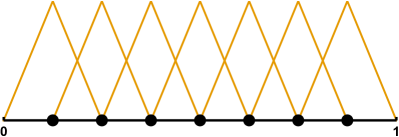
Figure 2: Nodal basis of hat functions with $N=7$ basis functions.

The examples given here in the introduction assume homogeneous boundaries for simplicity, i.e. they assume that the function value at the boundary is $0$. This restriction can easily be lifted by adding two additional basis functions, as we note below.

The basis functions for sparse grids in multiple dimensions are defined via a one-dimensional hierarchical basis. This hierarchical basis is equivalent to the nodal basis above, in the sense that they span the same space when using the same number of levels $n$, and one can efficiently convert between a them with cost $O(N\log N)$ without loss of information. Figure 3 shows such a hierarchical basis with $3$ levels.

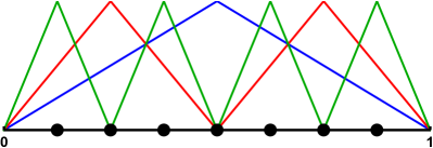
Figure 3: A hierarchical basis for the same space as in figure 2, using levels $\ell=0,1,2$.

A full set of nodal basis functions in multiple dimensions, corresponding to a full grid as used in a traditional finite differencing approximation, can be constructed as tensor product of one-dimensional nodal basis functions. A full set of hierarchical basis functions is likewise constructed as a tensor product.

II.1 The Hierarchical Sparse Basis

For an in-depth exposition on sparse grids, see bungartz2004sparse ; gerstner2011sparse . We will follow the conventions of the former. Historically, sparse grids were constructed from a basis of “hat” functions, defined by taking appropriate shifts and scalings of an initial hat function $\phi$:

$$\phi(x) :=\begin{cases}1-|x|,&\text{if}\ x\in[1,-1]\\ 0,&\text{otherwise}\end{cases}$$ (1)

$$\phi_{n,i}(x) =\phi\left(2^{n}\cdot\left(x-i\cdot 2^{-n}\right)\right)$$ (2)

to obtain a basis of functions supported on the unit interval $[0,1]$.

Higher order discretizations and respective sparse grids are obtained via appropriate piecewise polynomial basis functions. For simplicity, we only discuss second-order accurate discretizations in this section. We will introduce higher order approximations in section III later.

For a fixed level $n$, we denote this finite-dimensional space in terms of the nodal basis via the ansatz

$$\mathbf{V}_{n}:=\text{span}\left\{\phi_{n,i},\;1\leq i\leq 2^{n}-1\right\}.$$ (3)

Here $n$ is a positive integer, termed the level of resolution, which determines the granularity of the approximation. Each element $\phi_{n,i}$ is localized to within a radius $2^{-n}$ neighbourhood around the point $i\cdot 2^{-n}$. Here we use the letter $i$, ranging from $1$ to $2^{n}$, to refer to the respective node at level $n$.

For a function $u(x)$ on $[0,1]$, we can build its representation $\tilde{u}_{n}$ in this basis by

$$\tilde{u}_{n}(x)=\sum_{i=1}^{2^{n}-1}u_{n,i}\;\phi_{n,i}(x).$$ (4)

Here $u_{n,i}$ are the coefficients of $u$ in this basis representation on $\mathbf{V}_{n}$.

We find that $\mathbf{V}_{n}\subset\mathbf{V}_{n+1}$, and we can pick a decomposition

$$\mathbf{V}_{n}=\bigoplus_{\ell\leq n}\mathbf{W}_{\ell}.$$ (5)

so that the subspace $\mathbf{W}_{\ell}$ is complementary to $\mathbf{V}_{\ell-1}$ in $\mathbf{V}_{\ell}$, and $\mathbf{W}_{1}=\mathbf{V}_{1}$. $\mathbf{W}_{\ell}$ can also be defined explicitly as

$$\mathbf{W}_{\ell}:=\text{span}\left\{\phi_{\ell,i}:1\leq i\leq 2^{\ell}-1,\;i\,\text{odd}\right\}.$$ (6)

(We write $\phi_{n,i}$ when referring to all nodes $i$, and $\phi_{\ell,i}$ when referring only to odd $i$, which are the ones defining level $\ell$.)

When accounting for non-vanishing boundary conditions, we add in one more subspace denoted by $\mathbf{W}_{0}$ and defined to be $\text{span}\left\{x,1-x\right\}$. Note that these are the two only basis functions that don’t vanish on the boundary. For the sake of simplicity, we will ignore this subspace in this section.

A function $u$ can now be represented on $\mathbf{V}_{n}$ in terms of the $\phi_{\ell,i}$ basis as

$$\tilde{u}_{n}(x)=\sum_{\ell=0}^{n}\,\sum_{\begin{subarray}{c}i=1\\ i\;\text{odd}\end{subarray}}^{2^{\ell}-1}u_{\ell,i}\;\phi_{\ell,i}(x)$$ (7)

where the $u_{\ell,i}$ are again the coefficients of $u(x)$ in the hierarchical representation.

This new choice of basis functions, $\phi_{\ell,i}$ with $\ell$ ranging from $1$ to $n$ and $i$ odd, is called the hierarchical or multi-resolution basis for $\mathbf{V}_{n}$, because it includes terms from each resolution level. This basis is especially convenient when one wants to increase the resolution (i.e. the number of levels $n$), as one does not have to recalculate existing coefficients: Adding new levels with all coefficients set to $0$ does not change the represented function.

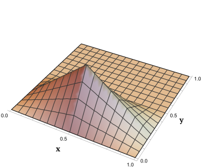
Figure 4: A tensor product of two hat functions, namely the one at level $\ell=0$ along $x$ and one at level $\ell=1,\,i=1$ along $y$. This corresponds to $\phi_{\mathbf{l}=(1,2),\,\mathbf{i}=(1,1)}$

In higher dimensions, the basis functions are obtained through the usual tensor product construction bungartz2004sparse . Now, the multi-resolution basis for $D$ dimensions consists of a set of basis functions $\phi_{\mathbf{l},\mathbf{i}}$ indexed by a $D$-tuple $\mathbf{l}$ of levels, called a multi-level, and a second tuple of elements $\mathbf{i}$, called a multi-node. The tensor product construction defines

$$\phi_{\mathbf{l},\mathbf{i}}(\mathbf{x}) =\prod_{d=1}^{D}\phi_{\mathbf{l}_{d},\mathbf{i}_{d}}(\mathbf{x}_{d}),$$ (8)

$$\mathbf{W}_{\mathbf{l}} :=\bigotimes_{d=1}^{D}\mathbf{W}_{\mathbf{l}_{d}}$$ (9)

$$\Rightarrow\mathbf{W}_{\mathbf{l}} =\text{span}\left\{\phi_{\mathbf{l},\mathbf{i}}:1\leq\mathbf{i}_{j}\leq 2^{\mathbf{l}_{j}},~{}\mathbf{i}_{d}~{}\text{odd for all }d\right\}$$ (10)

Figure 4 shows the two-dimensional basis function $\phi_{\mathbf{l}=(1,2),\mathbf{i}=(1,1)}$ as example. We write $\mathbf{k}\leq\mathbf{l}$ if the inequality holds for all components, i.e. $\forall d~{}\mathbf{k}_{d}\leq\mathbf{l}_{d}$. Then,

$$\mathbf{V}_{\mathbf{l}}:=\bigotimes_{d=1}^{D}\mathbf{V}_{\mathbf{l}_{j}}=\bigoplus_{\mathbf{k}\leq\mathbf{l}}\mathbf{W}_{\mathbf{k}}$$ (11)

Often in numerical approximation, the maximum level along each axis is the same number $n$, i.e. $\mathbf{l}=(n,n,\dots,n)$. In this case we write

$$\mathbf{V}_{n}^{D}:=\mathbf{V}_{(n,n,\dots,n)}=\bigoplus_{|\mathbf{k}|_{\infty}\leq n}\mathbf{W}_{\mathbf{k}}$$ (12)

We then finally define the sparse subspace$\mathbf{\hat{V}}^{D}_{n}\subseteq\mathbf{V}^{D}_{n}$ in terms of the hierarchical subspaces $\mathbf{W}_{\mathbf{k}}$. Rather than taking a direct sum over all the multi-levels $\mathbf{k}$, we define

$$\mathbf{\hat{V}}^{D}_{n}:=\bigoplus_{|\mathbf{k}|_{1}\leq n}\mathbf{W}_{\mathbf{k}}$$ (13)

to be the sparse space. Note that we use here the $1$-norm instead of the $\infty$-norm on the multi-level $\mathbf{k}$ to decide which multi-level basis indices to include. This selects only $1/d!$ of the possible multi-levels. This subspace selection is illustrated in figure 5 for $d=2,\;n=3$.

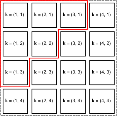
Figure 5: Illustration of the “sparsification” of a set of full grid coefficients for $D=2,\;n=4$ by removing all multi-levels past a certain $1$-norm. The dashed outline denotes the original multi-levels included in the full space, while the red line denotes only those included in the sparse space. Note that levels with higher indices contain exponentially more basis functions, so that the resulting reduction in dimensionality is significant, from $O(N^{D})$ to $O(N\log^{D-1}N)$, as elucidated in the main text in section II.2.

Because different levels have a different numbers of basis functions, and this process cuts off higher levels that have exponentially more basis functions than the lower ones, the resulting dimensionality reduction is significant. We discuss this in detail in the next subsection.

Sparse grids differ fundamentally from other discretization methods such as finite differences, spectral methods, finite elements, wavelets, or from adaptive mesh refinement for these methods. The difference is that sparse grids do not employ a tensor product ansatz in multiple dimensions, while all other methods customarily do.

II.2 Comparing Costs of Classical Grids

To construct a representation of a function living in $\mathbf{V}^{D}_{n}$, $2^{n}$ basis coefficients must be determined along each axis. This number is often referred to as the number of collocation points or grid points along that dimension, and we denote it by $N$. Its inverse $h=1/N$ is called the resolution.

In the full case, the dimension of $\mathbf{V}^{D}_{n}$ is the number of coefficients that must be stored for a representation up to level $n$ along each axis, and it is straightforward to see that we can write this as

$$\dim\mathbf{V}^{D}_{n}=O(2^{Dn})=O(N^{D}).$$ (14)

This exponential dependence of the size of this space on the number of spatial dimensions $D$ is the manifestation of the curse of dimensionality. On the other hand, the dimension of the sparse space is

$$\dim\mathbf{\hat{V}}^{D}_{n}=\sum_{|\mathbf{k}|_{1}\leq n}2^{|\mathbf{k}|_{1}}=O(2^{n}\,n^{D-1})=O(N\log^{D-1}N).$$ (15)

The sparse space uses far fewer coefficients, and suppresses the exponential dependence on $D$ to only the logarithmic term $\log N$.

Moreover, bungartz2004sparse ; zenger1991sparse show that the two-norm of the error of an approximation $\tilde{u}_{\text{full}}\in\mathbf{V}^{D}_{n}$ of a function $u\in H_{2}([0,1]^{D})$ in the Sobolev space scales as

$$||u(\mathbf{x})-\tilde{u}_{\text{full}}(\mathbf{x})||_{2}=O(N^{-2})$$ (16)

while for $\tilde{u}_{\text{sparse}}$ in the corresponding sparse space, it is

$$||u(\mathbf{x})-\tilde{u}_{\text{sparse}}(\mathbf{x})||_{2}=O(N^{-2}\,\log^{D-1}N).$$ (17)

This means that the error increases only by a logarithmic factor, showing the significant advantage of the sparse basis over the full basis for all dimensions greater than one.

We define the $\varepsilon$-complexity traub1980 ; bungartz2004sparse of a scheme as the error bound $\varepsilon$ that can be reached with a given number of coefficients $P$. A full grid has an $\varepsilon$-complexity in the $L_{2}$ norm of

$$\varepsilon^{\mathrm{full}}_{L_{2}}(P)=O(P^{-2/D})$$ (18)

which decreases quite slowly for larger dimensions. The sparse grid, on the other hand, does considerably better with

$$\varepsilon^{\mathrm{sparse}}_{L_{2}}(P)=O(P^{-2}\,\log^{3(D-1)}P).$$ (19)

Though the logarithmic factor is significant enough that it cannot be ignored in practice, even in high dimensions this still represents a significant reduction in the number of coefficients required.

This can be generalized to higher-order finite differencing and corresponding hierarchical grids. In this case, the power $P^{-2}$ improves to $P^{-k}$ correspondingly for both full and sparse grids.

For comparison, we also discuss the accuracy of single-domain spectral representations. These have an error of

$$||u(\mathbf{x})-\tilde{u}_{\text{spectral}}(\mathbf{x})||_{2}=O(\exp(-N))$$ (20)

where the linear number of coefficients $N$ defines the spectral order. Its epsilon-complexity is then

$$\varepsilon^{\mathrm{spectral}}_{L_{2}}(P)=O(\exp(-P^{1/D})).$$ (21)

A priori, single-domain spectral methods offer a much better accuracy/cost ratio than either full or sparse grids. However, single-domain spectral representations are typically only useful for smooth functions: The sampling theorem requires $N\gtrsim 2L/h$, where $L$ is the size of the domain and $h$ is the smallest feature of the function that needs to be resolved. Functions with $L/h\gg 1$ are called not smooth. In this case, the minimum required number of coefficients $P$ is determined not by the accuracy $\varepsilon$, but rather by the necessary minimum resolution, annihilating the major advantage of spectral methods. In this case, multi-domain spectral representations such as Discontinuous Galerkin Finite Elements are preferable, as we discuss below.

III The Discontinuous Galerkin Sparse Basis

We review here the work of Guo and Cheng guo2016 and Wang et al. wang2016 on how one can generalize this sparse grid construction beyond hat functions or their higher-order finite-differencing (FD) equivalents. (Although we only discussed second-order accurate sparse grids in the previous section, these can be extended to arbitrary orders in a straightforward manner.) Then we introduce a scheme for defining a derivative operator in a manner similar to the Operator-Based Local Discontinuous Galerkin (OLDG) method developed in miller2016 .

The main advantage of DGFE sparse grids over classical, finite-differencing based sparse grids is the same as the advantage that regular DGFE discretizations possess over finite-difference discretization: (1) For high polynomial orders (say, $k>8$), the collocation points within DGFE elements can be clustered near the element boundaries, leading to increased stability and accuracy near domain boundaries. (2) The derivative operators for DGFE discretizations exhibit a block structure, which is computationally significant more efficient than the band structure found in higher-order finite differencing operators. (3) Basis functions are localized in space, which allows for $hp$ adaptivity. Corresponding Adaptive Mesh Refinement (AMR) algorithms for FD discretization do not allow adapting the polynomial order.

However, DGFE methods also have certain disadvantages. In particular, the Courant-Friedrichs-Lewy (CFL) condition on the maximum time step size is typically more strict, intuitively because the collocation points cluster near element boundaries.

III.1 Constructing Galerkin Bases

The space $\mathbf{V}_{n}$ of hat-functions in one dimension is equivalent to the span of $2^{n}$ hat functions defined on sub-intervals of length $2^{-n}$ that subdivide $[0,1]$ into $2^{n}$ intervals of the form $I_{i,n}:=[(i-1)\cdot 2^{-n},\,i\cdot 2^{-n}]$. A natural generalization of this is to consider the linear sum of spaces $P_{k}(I_{i,n})$ of functions that, when restricted to $I_{i,n}$ become polynomials of degree less than $k$, and are zero everywhere outside.

This leads to a space of basis functions on $[0,1]$ called $\mathbf{V}_{n,k}$, defined as:

$$\mathbf{V}_{n,k}:=\bigoplus_{i=1}^{2^{n}}P_{k}(I_{i,n}).$$ (22)

Note that $\dim\mathbf{V}_{n,k}=k\cdot 2^{n}$. The analogue of the modal basis above is the following collection of basis vectors

$$\{h_{n,i,m}:1\leq i\leq 2^{n},\;1\leq m\leq k\}$$ (23)

so that for a given $i$, each $h_{n,i,m}$ is supported only on the interval $I_{i,n}$ from before, and together they constitute a basis of $k$ orthonormal polynomials of degree less than $k$ on that interval. In this case, $h_{n,i,m}$ can be identified as an appropriate shift and scale of the $m$-th Legendre polynomial with support only on $[-1,1]$. We then obtain the orthonormal basis:

$$h_{n,i,m}(x):=\begin{cases}2^{(n+1)/2}\,P_{m}\left(2^{n}\cdot(x-i\cdot 2^{-n})\right)&\text{if}~{}x\in I_{i,n}\\ 0&\text{otherwise.}\end{cases}$$ (24)

As before, $\mathbf{V}_{n-1,k}\subset\mathbf{V}_{n,k}$, and so we can again construct a hierarchical decomposition by choosing a complement to $\mathbf{V}_{n-1,k}$ in $\mathbf{V}_{n,k}$. In fact, we can obtain this decomposition canonically by using an inner product on the space of piecewise polynomial functions. For $f,g$ in this space, define:

$$\left<f,g\right>:=\int_{[0,1]}f(x)\,g(x)\,dx.$$ (25)

Then letting $\mathbf{W}_{n,k}$ be the orthogonal complement to $\mathbf{V}_{n-1,k}$ in $\mathbf{V}_{n,k}$, we obtain

$$\mathbf{V}_{n,k}=\mathbf{V}_{n-1,k}\oplus\mathbf{W}_{n,k},\qquad\mathbf{W}_{n,k}\perp\mathbf{V}_{n-1,k}.$$ (26)

From this we can construct a hierarchical orthonormal basis of functions for the entire space $\mathbf{V}_{n,k}$:

$$v_{\ell,i,m}(x)\qquad 0\leq\ell\leq n,\;1\leq i\leq 2^{l},\;1\leq m\leq k.$$ (27)

Here $\ell$ is the level and $i$ is the element at level $l$. $m$ is called the mode and indexes the $k$ orthogonal polynomials on the subinterval corresponding to $(l,i)$. For a more explicit construction of this basis, see wang2016 ; alpert1991 .

Figure 6 illustrates resulting polynomials for $k=3$. Unlike in the FD basis before, we now directly allow for non-vanishing boundary values, and the level thus now ranges from $0$ to $n$ rather than $1$ to $n$.

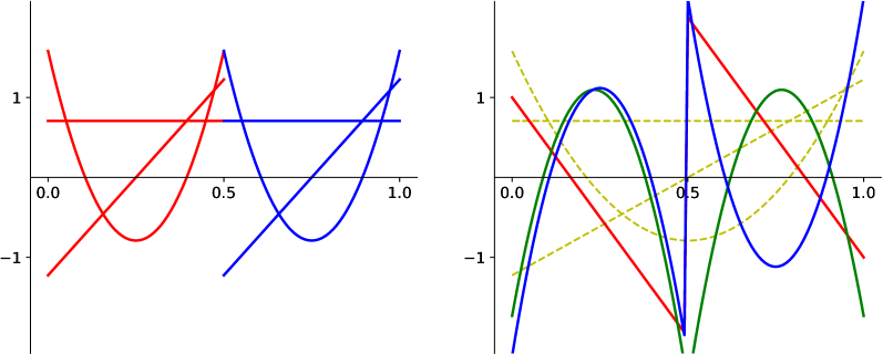
Figure 6: Illustration of two different orthogonal bases for resolving the two half intervals of $[0,1]$, corresponding to resolution level $1$. On the left are piecewise Legendre polynomials for the original discontinuous Galerkin (DG) basis. On the right are the zeroth and first levels of the multi-resolution basis as $k=3$. Level $0$ modes consist of Legendre polynomials, shown as dashed yellow lines. Higher levels are shifts/scalings to the appropriate subintervals of the three level $1$ basis modes drawn in red, green, and blue. This construction is comparable to $h$-refinement in Adaptive Mesh Refinement (AMR) schemes.

In the $D$-dimensional case, we proceed as before to apply the tensor product construction with the conventions of the previous Section II.1:

$$v_{\mathbf{l},\mathbf{i},\mathbf{m}}(\mathbf{x}) =\prod_{d=1}^{D}v_{\mathbf{l}_{d},\mathbf{i}_{d},\mathbf{m}_{d}}(\mathbf{x}_{d}),$$ (28)

$$\mathbf{W}_{\mathbf{l}}^{k} =\bigotimes_{d=1}^{D}\mathbf{W}_{\mathbf{l}_{d}}^{k}.$$ (29)

The basis $v_{\mathbf{l},\mathbf{i},\mathbf{j}}$ spans the full discontinuous Galerkin grid space in $D$ dimensions. As before, $\mathbf{l},\mathbf{i}$ are $D$-tuples of levels and elements called the multi-level and multi-element. $\mathbf{m}$ is a $D$-tuple of modes called a multi-mode. We can write this space in terms of its level decomposition as:

$$\mathbf{V}_{n,k}^{D}=\bigoplus_{|\mathbf{l}|_{\infty}\leq n}\mathbf{W}_{\mathbf{l}}^{k}.$$ (30)

The corresponding sparse vector space is then defined as before wang2016 ; guo2016 by using the $1$-norm of this integer index space to select only a subset of basis functions:

$$\hat{\mathbf{V}}_{n,k}^{D}=\bigoplus_{|\mathbf{l}|_{1}\leq n}\mathbf{W}_{\mathbf{l}}^{k}.$$ (31)

We will use this space in our tests and examples to efficiently construct solutions for hyperbolic PDEs in the next section.

III.2 Comparing Costs of Galerkin Grids

Analogous to equations (14) and (15) in section II.2, we describe here the cost (number of basis functions) and errors associated with full and sparse DG spaces.

$$\dim\mathbf{V}_{n,k}^{D} =O(2^{Dn}\,k^{D})=O(N^{D}\,k^{D})$$ (32)

$$\dim\hat{\mathbf{V}}_{n,k}^{D} =O(2^{n}\,k^{D}\,n^{D-1})=O(N\,k^{D}\,\log^{D-1}N).$$ (33)

This shows that a sparse grid reduces the cost significantly as the resolution $N$ is increased, while our construction has no effect on the way the cost depends on the polynomial order $k$. In the big-$O$ notation, these cost functions omit large constant factors that depend on the number of dimensions $D$.

Further, from schwab2008 we obtain the DGFE analogues of equations (16) and (17) for the $L^{2}$-norm of the approximation error:

$$||u(\mathbf{x})-\tilde{u}_{\text{full}}(\mathbf{x})||_{2} =O(N^{-k})$$ (34)

$$||u(\mathbf{x})-\tilde{u}_{\text{sparse}}(\mathbf{x})||_{2} =O(N^{-k}\,\log^{D-1}N).$$ (35)

which is equivalent to (16) and (17), except that we now achieve a higher convergence order $k$ instead of just $2$: The error found in sparse grids is only slightly (by a logarithmic factor) larger than that in full grids.

This yields the resulting $\varepsilon$-complexities:

$$\varepsilon_{L^{2}}^{\text{full DG}}(P) =O\left(P^{-k/D}\right)$$ (36)

$$\varepsilon_{L^{2}}^{\text{sparse DG}}(P) =O\left(P^{-k}\,k^{Dk}\,\log^{(k+1)(D-1)}P\right)$$ (37)

This is consistent with an analogous estimate in bungartz2004sparse . Again, the sparse grid DG case provides a significant improvement over the full grid DG case. We compare these scalings graphically in figure 7 for $D=3$.

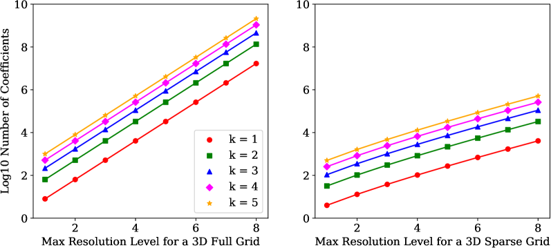
Figure 7: The number of coefficients vs. the maximum level, comparing full (left) and sparse (right) grids. This shows the storage (memory) cost, on a log scale, vs. the maximum level of resolution $n$ of a degree $k$ Galerkin scheme in three dimensions. Shown for both the full and sparse spaces, i.e. $\dim\mathbf{V}_{n,k}$ and $\dim\hat{\mathbf{V}}^{k}_{n}$ for $D=3$. The reduction in cost is evident. The slight downward curvature in the right figure is caused by the logarithmic term, which remains relevant in practice for the shown number of levels.

We note that, in general, spectral methods can offer superior accuracy, but they also suffer from the curse of dimensionality, and representing non-smooth functions requires high orders since exponential convergence is lost in this case. If only a single spectral level is used, then DG sparse grids are equivalent to a spectral method. DG sparse grids are thus a true superset of spectral discretizations.

III.3 Constructing the Derivative Operator

To solve hyperbolic PDEs, we define a derivative operator on the multi-dimensional sparse basis. This is the main contribution of this paper. To do this, we proceed in steps:

1. Define the derivative on the one-dimensional Galerkin space $\mathbf{V}_{n,k}$ in terms of the modal basis of Legendre polynomials.

2. Express this operator in the one-dimensional hierarchical basis.

3. Using the tensor-product construction, define the derivative matrix elements in the full multi-dimensional basis $\mathbf{V}_{n,k}^{D}$.

4. Restrict (project) this operator to the sparse subspace. Since our basis functions are orthonormal, this corresponds to only calculating matrix elements between basis functions in $\hat{\mathbf{V}}_{n,k}^{D}$, and ignoring (i.e. discarding) those matrix elements that would lead out of this subspace. This step introduces an additional approximation into our scheme.

To define the derivative in the standard Galerkin basis in one dimension, we follow the methods outlined in miller2016 . For a given maximum number of levels $n$ and degree $k$, let $h_{n,i,m}$ be as before.

The derivative operator is then defined in the weak sense:

$$\int_{[0,1]}h_{n,i,m}(x)\,\frac{df}{dx}(x)\,dx =\int_{I_{i,n}}h_{n,i,m}(x)\,\frac{df}{dx}(x)\,dx$$ (38)

$$=\Big{[}h_{n,i,m}(x)\,f(x)\Big{]}_{(i-1)2^{-n}}^{i2^{-n}}-\int_{I_{i,n}}f(x)\,\frac{dh_{n,i,m}}{dx}(x)\,dx$$

Because the $h_{n,i,m}$ are discontinuous at the two boundary points, where they jump from zero to nonzero values, we define $h_{n,i,m}((i-1)2^{-n})$ and $h_{n,i,m}(i2^{-n})$ to be the average of the two, namely half the endpoint value, following cohen2017 ; hesthaven2010 . (arnold2000 contains also a very good description of the weak formulation for derivatives, although it considers only elliptic systems.)

This choice of the average corresponds to a central flux. The same choice was made in miller2016 , where the authors argue that this is a convenient “black box” choice that works for many systems of strongly hyperbolic PDEs, and is not restricted to manifestly flux-conservative formulations. Another reason for this choice here is that it results in a linear operator, which allows formulating and applying the derivative operator in modal space (i.e. on individual modes) instead of having to reconstruct the function values at element interfaces. The latter is quite complex to define, as finer levels have element interfaces at locations in the interior of coarser levels (see the right subfigure in figure 6), and – different from standard DG methods – in a hierarchical basis all levels are “active” and contribute to the representation simultaneously.

The boundary term then becomes:

$$\frac{1}{2}\lim_{\epsilon\to 0^{+}}\left[f\!\left(i2^{-n}-\epsilon\right)\,h_{n,i,m}\!\left(i2^{-n}-\epsilon\right)-f\!\left((i-1)2^{-n}+\epsilon\right)\,h_{n,i,m}\!\left((i-1)2^{-n}+\epsilon\right)\right]$$ (39)

while in the second integral, $h_{n,i,m}$ is treated exactly as a polynomial function. Its derivative is then exactly computable. By knowing the basis representation of $f$ in terms of $h_{n,i,m}$, we can obtain an explicit matrix form of the derivative operator via

$$\mathcal{D}_{i,m;\,i^{\prime},m^{\prime}}:=\int_{[0,1]}h_{n,i,m}(x)\,\frac{dh_{n,i^{\prime},m^{\prime}}}{dx}(x)\,dx.$$ (40)

This matrix will be a sum of two matrices, as above: One term corresponding to the discontinuity terms at the boundary, and the second term corresponding to the regular derivative operator on the smooth polynomial functions in the interior.

By orthogonally transforming $h_{n,i,j}$ into the hierarchical Galerkin basis $v_{\ell,i,j}$ through a transformation $Q$, we can conjugate this derivative operator into its hierarchical form $\mathcal{D}^{\text{hier}}=QDQ^{T}$. We generalize this operator to higher dimensions through the standard tensor product construction. The partial derivative operator $\partial_{a}$ is represented by the derivative operator $\mathcal{D}_{a}^{\text{full}}$ acting on the basis $v_{\mathbf{l},\mathbf{i},\mathbf{j}}$ as

$$\mathcal{D}^{\text{full}}_{a}(v_{\mathbf{l},\mathbf{i},\mathbf{j}})=\left[\mathcal{D}^{\text{hier}}v_{\mathbf{l}_{a},\mathbf{i}_{a},\mathbf{j}_{a}}\right]\,\prod_{m\neq a}v_{\mathbf{l}_{m},\mathbf{i}_{m},\mathbf{j}_{m}}.$$ (41)

The last step is to restrict this full derivative operator to the sparse space. We obtain $\mathcal{D}^{\text{sparse}}_{a}$ from $\mathcal{D}^{\text{full}}_{a}$ by restricting the latter to the sparse basis space. Note, however, that $\mathcal{D}^{\text{full}}_{a}$ does not preserve the sparse space, as it has nonzero matrix entries mapping sparse to non-sparse basis elements. (This is also the case for the 1D derivative operator $\mathcal{D}^{\text{hier}}$, which doesn’t stabilize $\mathbf{V}_{n,k}\subset\mathbf{V}_{n+1,k}$.) When restricting the derivative matrix to $\mathbf{V}_{n,k}$, we ignore those components of the operator that map outside of $\mathbf{V}_{n,k}$. We shall do the same here, and define

$$\mathcal{D}^{\text{sparse}}_{a}=\text{Proj}_{\hat{\mathbf{V}}_{n,k}^{d}}\mathcal{D}^{\text{full}}_{a}.$$ (42)

This will be the working definition for our derivative operator in the sparse basis.

Further, the matrix representing this derivative operator is itself sparse. This is clear upon noting that $\mathcal{D}_{a}^{\text{full}}$ only acts on the $a$-indexed components of the basis $v_{\mathbf{l},\mathbf{i},\mathbf{m}}$. Thus on a specific $v_{\mathbf{l},\mathbf{i},\mathbf{m}}$, $\mathcal{D}^{\text{sparse}}_{a}$ has a nonzero matrix entry against another basis vector exactly when $\mathcal{D}^{\text{hier}}$ does on the one-dimensional basis along the $a$-th axis. Looking at $\mathcal{D}^{\text{hier}}_{a}$ in one dimension, since a given element at $(\ell,i)$ will only have nonzero derivative entry against basis vectors supported either on its element, its neighbouring elements, or elements that contain it at lower $\ell$, this gives a total of $O(\log N)$ nonzero entries for the derivative matrix acting on $v_{\mathbf{l},\mathbf{i},\mathbf{m}}$ . Thus we get a total of $O(P\log N)\approx O(P\log P)$ nonzero matrix entries in general, and this log-linearity is numerically verified in figure 8. This sparse structure is crucially important when solving PDEs, as it determines the run-time cost of the algorithm.

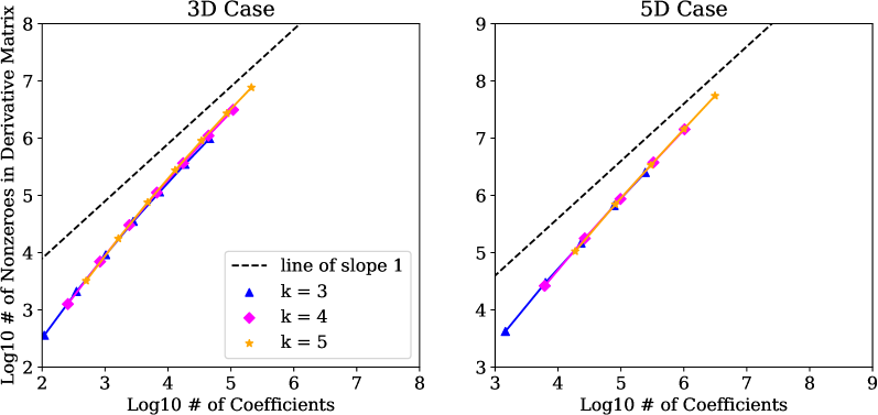
Figure 8: This figure illustrates that the number of nonzero coefficients in the sparse derivative matrix scales as $P\log P$ where $P$ is the total number of coefficients stored at a given resolution and order. Note that the slope of the graphs in this log-log plot tends to $1$ as the number of coefficient grows, indicating a scaling that is much closer to $O(P)$ than $O(P^{2})$. This indicates that the derivative matrix is sparse, confirming our $O(P\log P)$ estimate (see main text).

For PDEs with periodic boundary conditions, the 1D derivative operator, from which the full and sparse derivatives are constructed, will have the boundary terms in the integration by parts (38) overlap at the opposite endpoints $0$ and $1$. This turns the interval $[0,1]$ into the torus $T^{1}$.

IV Evolving a Scalar Wave in the DGFE Basis

Using the sparse derivative operator that we have constructed, we turn to solving the scalar wave equation (in a flat spacetime) as example and test case. This equation can be reduced to first order in time as

$$\begin{matrix}\dot{\varphi}(\mathbf{x},t)=\psi(\mathbf{x},t)~{}~{}~{}\,\\ \dot{\psi}(\mathbf{x},t)=\nabla^{2}\varphi(\mathbf{x},t)\end{matrix}~{}\Rightarrow~{}\frac{d}{dt}\begin{pmatrix}\varphi\\ \psi\end{pmatrix}=\begin{pmatrix}0&\mathbf{1}\\ \nabla^{2}&0\end{pmatrix}\begin{pmatrix}\varphi\\ \psi\end{pmatrix}.$$ (43)

We then use the DGFE basis to represent this as

$$\varphi(\mathbf{x},t)=\sum_{\mathbf{l},\mathbf{i},\mathbf{j}}\varphi_{\mathbf{l},\mathbf{i},\mathbf{j}}(t)\,v_{\mathbf{l},\mathbf{i},\mathbf{j}}(\mathbf{x}), \qquad\psi(\mathbf{x},t)=\sum_{\mathbf{l},\mathbf{i},\mathbf{j}}\psi_{\mathbf{l},\mathbf{i},\mathbf{j}}(t)\,v_{\mathbf{l},\mathbf{i},\mathbf{j}}(\mathbf{x}),$$ (44)

$$\nabla^{2}\to\sum_{a}\, \,\mathcal{D}_{a}^{\text{sparse}}\cdot\mathcal{D}_{a}^{\text{sparse}}.$$ (45)

As written, this representation is exact – it only corresponds to a particular basis choice. We then introduce a cut-off for the number of levels $n$, which introduces an approximation error.

Here, $\varphi_{\mathbf{l},\mathbf{i},\mathbf{j}}$ and $\psi_{\mathbf{l},\mathbf{i},\mathbf{j}}$ are the coefficients representing $\varphi,\psi$. The problem is now framed as a set of coupled first-order ordinary differential equations (ODEs). Such ODEs can be solved in a straightforward manner via a wide range of ODE integrators e.g. of the Runge-Kutta family.

Since the derivative and Laplacian operators are sparse matrices, and since the maximum allowable time step scales with the resolution $h$ and thus with the linear problem size $N$ due to the Courant-Friedrichs-Lewy (CFL) criterion, the overall cost to calculate a solution scales as $O(N^{2}\log^{D-1}N)$, which is significantly more efficient than the $O(N^{D+1})$ scaling for a full grid. Here $D$ is the number of spatial dimensions. In principle it is possible to employ a sparse space-time discretisation as well, reducing the cost further to $O(N\log^{D}N)$. However, this will require a more complex time evolution algorithm instead of the ODE solver we employ, and we thus do not investigate this approach in this paper.

Initial conditions for this time evolution are given by the coefficients of the initial position and velocity of the wave $\varphi_{0},\psi_{0}$. This requires projecting given functions into the sparse space. (Later, time evolution proceeds entirely in coefficient space.) Accurately projecting onto the basis functions requires (in practice) a numerical integration for each coefficient. If one is satisfied with the accuracy and convergence properties of sparse grids, then one can replace this numerical integration with sampling the given function at the collocation points of the DG basis functions, as is often done. However, we do not want to make such assumptions in this paper, and thus use a (more accurate, and more expensive) numerical integration to properly project the initial conditions onto the basis functions.

It is advantageous (the calculation is simpler) if the initial conditions can be cast as sums of tensor products of 1D functions. By projecting these individual components of the solution in 1D, and then applying the tensor construction to those 1D coefficients, we can recover the coefficients of the full $D$-dimensional function. This yields a considerable speedup of the initial data construction, as all integrations only need to be performed in 1D.

Such a construction can in particular be applied to all sine waves of the form $\sin(\mathbf{k}\cdot\mathbf{x}-\phi)$ by expressing them as sums of products of sines and cosines in one variable.

As stated above, in the general case, a sparse integrator (e.g. based on sparse grids!) could be used to avoid concerns with the cost of high-dimensional integration. Out of caution we avoid this since we do not want to use sparse methods to test our sparse discretization – we want to test via non-sparse methods only.

We present results in section VI below, after briefly introducing the Julia package we developed to perform these calculations in section V.

V Overview of the Open-Source Package

The Julia code for performing interpolation and wave evolution using the sparse Galerkin bases outlined in this paper is publicly available as open source under the “MIT” licence at

https://github.com/ABAtanasov/GalerkinSparseGrids.jl

To obtain the basis coefficients resulting from projecting a function f in D dimensions at degree k and level n, we use the command coeffs_DG as follows:

⬇

using GalerkinSparseGrids

D = 2; k = 3; n = 5;

f = x -> sin(2*pi*x[1])*sin(2*pi*x[2])

full_coeffs = coeffs_DG(D, k, n, f; scheme="full" )

sparse_coeffs = coeffs_DG(D, k, n, f; scheme="sparse")

Obviously, calling full_coeffs is much more expensive than sparse_coeffs, and should only be used to compare cost and accuracies.

This creates a dictionary-like data structure for efficient access to coefficients at the various levels and elements. The coefficients at each level/element are then stored as dense array for efficiency. Given such a dictionary of coefficients, we can evaluate the function at a D-dimensional point x using reconstruct_DG.

⬇

full_val = reconstruct_DG(full_coeffs , x)

sparse_val = reconstruct_DG(sparse_coeffs, x)

The explicit function representation can then be written (given access to sparse_coeffs) as:

⬇

f_rep = x -> reconstruct_DG(sparse_coeffs, [x...])

We also include a Monte-Carlo integration function mcerr for a quick calculation of the error between the exact and the computed function

⬇

mcerr(f::Function, g::Function, D::Int; count = 1000)

This provides a good estimate the $L^{2}$ norm of the error between $f$ and $g$. The data points in this paper representing errors were calculated using this method. For example, to generate one of the data points in figure 9, one uses

⬇

sparse_coeffs = coeffs_DG(D, k, n, f)

f_rep = x -> reconstruct_DG(sparse_coeffs, [x...])

err = mcerr(f, f_rep, D)

For algorithms such as time evolution and differentiation, the dictionary-like coefficient tables are converted into vectors (one-dimensional arrays), so that the derivative operators act as multiplication by a sparse matrix, and all operations can be performed efficiently. To convert a dictionary dict of coefficient tables to a single coefficient vector vcoeffs (or vice versa) we use

⬇

vcoeffs = D2V(D, k, n, dict; scheme="sparse")

dict = V2D(D, k, n, vcoeffs; scheme="sparse")

Given a vector of coefficients, one can easily compute the $L^{2}$ norm of the representation (since the basis is orthonormal) by using the built-in Julia function

⬇

L2_norm = norm(vcoeffs)

Explicitly, one can obtain the derivative operator matrix $\mathcal{D}_{a}$ as:

⬇

D_matrix(D::Int, a::Int, k::Int, n::Int; scheme="sparse")

The full list of $\mathcal{D}_{a},a\in[1,D]$ matrices can be computed through:

⬇

grad_matrix(D::Int, k::Int, n::Int; scheme="sparse")

The corresponding Laplacian operator is the sum of the squares of this list, and is given by

⬇

laplacian_matrix(D::Int, k::Int, n::Int; scheme="sparse")

All of these operators are meant to act on the appropriate vectors of coefficients.

To solve the wave equation given initial conditions, we provide the following function:

⬇

wave_evolve(D::Int, k::Int, n::Int,

f0::Function, v0::Function,

time0::Real, time1::Real;

order="45", scheme="sparse")

Using the representation of the initial data and Laplacian operator given in equations (44) and (45), this represents the $D$-dimensional wave equation with initial conditions f0 for $\varphi$ and v0 for $\psi$ by a set of linearly coupled first order ODEs, enforcing periodicity boundary conditions.

It is straightforward to modify this code to solve different systems of equations. To support non-linear systems, one needs to introduce collocation points for the DG modes and perform the calculation in the respective nodal basis. While this is not yet implemented, it is well-known how to do this, as is e.g. done in miller2016 .

This system can then be evolved by any integrator in the various Julia packages for ordinary differential equations. In the present package, we chose to use ode45 and ode78 from the ODE.jl package odejl .

For example, to solve a standing wave in 2D from time t_0 to time t_1 with polynomials of degree less than k on each element, using a sparse depth n, and with the ode78 ODE integrator:

⬇

D = 2; k = 5; n = 5;

f0 = x->sin(2*pi*x[1])*sin(2*pi*x[2])

v0 = 0

soln = wave_evolve(D, k, n, f0, v0, 0, 0.25; order="78")

The array structure of soln is like any solution given by the ODE.jl package. soln will have three components. The first is an array of times at which the timestep was performed. The second is an array of coefficients corresponding to the evolution of the initial data f0 at those time points. The third is an array of coefficients corresponding to the evolution of the initial data v0.

To calculate the final error vs. the exact solution for time-evolving the standing sine wave from before, we write

⬇

f_exact = x -> cos(2*pi*x[1])*sin(2*pi*x[2])

f_rep = x -> reconstruct_DG(soln[2][end], [x...])

err = mcerr(f_exact, f_rep, D)

In the case one wants to evolve specifically a travelling wave, we provide the function

⬇

travelling_wave_solver(k::Int, n::Int, m::Array{Int,1},

time0::Real, time1::Real;

scheme="sparse", phase=0.0, A=1.0, order="45")

to evolve a travelling wave with wave number 2*pi*m, amplitude A, and phase phase from time t0 to time t1. This function was used to generate several of the plots of wave evolution error in this paper. It makes use of being able to write any sine-wave as a sum of products of one-dimensional sine waves along each axis. Such a construction can be done explicitly using the method

⬇

tensor_construct(D::Int, k::Int, n::Int, coeffArray; scheme="sparse")

which takes $D$ vectors coefficient and constructs the coefficient of their corresponding $D$-dimensional tensor product function.

More documentation is available in the Github repository and as part of the source code.

VI Results

The Galerkin bases and derivative operators constructed above allow representing arbitrary functions, calculating their derivatives, calculating norms, solving PDEs, and evaluating the solution at arbitrary points, as is the case with any other discretization method.

We focus here on the scalar wave equation as simple (and linear) example application. Using the methods developed in the prior sections, we use the Galerkin sparse grid package to calculate efficient and accurate representations in $3$, $5$, and $6$ dimensions, and we evolve the wave equation in time in $3+1$, $5+1$, and $6+1$ dimensions. At this accuracy, this would have been prohibitively expensive using full grid methods. All calculations were performed on a single (large) workstation.

In the following discussion, all errors have been calculated via a Monte Carlo integration to evaluate integrals of the form

$$\int_{[0,1]^{D}}\left|u^{*}(\mathbf{x})-\tilde{u}(\mathbf{x})\right|^{2}d^{D}\mathbf{x}$$ (46)

for $u^{*}$ the analytically known solution and $\tilde{u}$ the DGFE approximation to the solution. The $L^{2}$ error is output as the square root of the above quantity. We use approximately $1000$ points, enough to guarantee convergence to satisfactory precision for error measurement in our case. We tested that using more sampling points did not noticeably change the results.

VI.1 Approximation Error for Representing Given Functions

We begin by evaluating the approximation error made when representing a given function with a sparse basis at a particular cut-off level. We choose as function a sine wave of the form

$$f(\mathbf{x}) = A\cos(\mathbf{k}\cdot\mathbf{x}+\phi)$$ (47)

with $A=1.3,\;\phi=0.4$, using $\mathbf{k}=2\pi\cdot[1,2,-1]$ in 3D and $\mathbf{k}=2\pi\cdot[1,0,-1,2,1]$ in 5D. We also employ periodic boundary conditions. These first tests do not yet involve derivatives or time integration.

Figure 9 compares the accuracy achieved with a particular number of coefficients for full and sparse grids. As expected, sparse grids are more efficient (in the sense of the accuracy-to-cost ratio), and this efficiency increases for higher resolutions. As also expected, this effect is even more pronounced in the $D=5$ case.

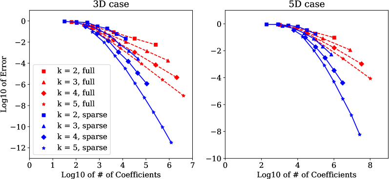
Figure 9: Comparing approximation errors as a function of the number of coefficients for $D=3$ (left) and $D=5$ (right) for values of the polynomial order $k$ from $1$ to $5$. We vary the number of coefficients by varying the level $n$. Even at moderate scales ($10^{5}$ coefficients), sparse grids for $k=5$ exhibit errors that are more than $4$ orders of magnitude smaller than their full counterparts. Particularly noteworthy here is the fact that the accuracy gain from higher polynomial order $k$ in the sparse scheme is far more significant than in the full scheme. This shows significant promise for higher-order sparse Galerkin methods. See main text for more details.

		sparse grid					full grid
$n$	Avg.	time	Mem.	usage	Approx. Error	Avg.	time	Mem.	usage	Approx. Error
1	0.80	ms	7.8	MB	$1.1\cdot 10^{-1}$	9.7	ms	68	MB	$6.3\cdot 10^{-2}$
2	7.6	ms	54	MB	$9.9\cdot 10^{-3}$	1.1	s	5.0	GB	$2.6\cdot 10^{-3}$
3	40	ms	270	MB	$8.0\cdot 10^{-4}$	?		?		?
4	220	ms	1.3	GB	$5.0\cdot 10^{-5}$
5	1.0	s	5.5	GB	$2.6\cdot 10^{-6}$
6	4.5	s	23	GB	$1.6\cdot 10^{-7}$
7	21	s	97	GB	$5.9\cdot 10^{-9}$

Table 1: Comparing run times and memory usage for sparse and full grids. This table shows the average run time of applying the Laplacian operator to an order $k=5$ representation of a waveform in $D=5$ dimensions, for various levels $n$, as well as the memory needed to store the Laplacian matrix and coefficient vectors. Levels $n=3$ and above required more than 200 GByte of memory for a full grid and could not be run on a single node. (Our implementation does not yet support distributed-memory systems.) As described by equations (34) and (35), sparse grids have a slightly lower accuracy than full grids for the same number of levels (by a factor logarithmic in $n$).

Even in two dimensions, the sparse Galerkin basis already provides a considerable advantage in efficiency. For the sake of visual intuition, we show the approximation error of representing a sine wave in 2D by Galerkin sparse grids of in figure 10, for polynomial order $k=3$ and sparse level $n=5$.

Table 1 compares run times and memory usage between sparse and full grids, run on a single high-memory node of the Grace cluster at Yale. It is evident that sparse grids require far fewer resources than full grids for the same accuracy.

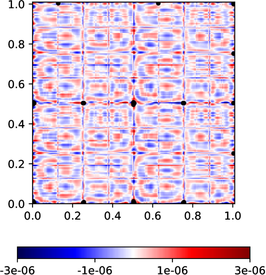
Figure 10: Approximation error (difference to exact value) of a sine wave $\varphi(\mathbf{x})=A\cos(\mathbf{k}\cdot\mathbf{x}+\phi)$ on $[0,1]\times[0,1]$ with $A=1.3,\;\phi=0.4,$ and $\mathbf{k}=2\pi\cdot[1,2]$ in 2D for $k=5,\;n=5$. The small discontinuities typically introduced at element boundaries and corners by DGFE methods are clearly visible. The maximum absolute error is about $10^{-5}$; we clip the colourmap to $3\cdot 10^{-6}$ for clarity, and the small saturated (black) regions where the error is larger are clearly visible. Contrary to the naive assumption, the error is not the largest in the interior (away from the boundaries), where the sparse grid structure has removed most collocation points.

VI.2 Approximation Error in Time Evolution

Beyond just representing given functions, figures 11 and 12 demonstrate the accuracy of evolving a scalar wave using DGFE sparse grids. After projecting the initial position and velocity of a travelling wave in 3 and 5 dimensions onto the sparse basis, we evolve the system in time using the derivative matrices $\mathcal{D}^{\text{sparse}}_{a}$ and the wave evolution scheme described in Sections III.3 and IV, respectively.

Initial conditions for the evolution are

$$\varphi(\mathbf{x},0)=\cos(\mathbf{k}\cdot\mathbf{x}+\phi),~{}\psi(\mathbf{x},0)=-\omega\sin(\mathbf{k}\cdot\mathbf{x}+\phi)$$

where here $\mathbf{k}$ is a wave number vector compatible with the periodic boundary conditions and $\omega=|\mathbf{k}|$.

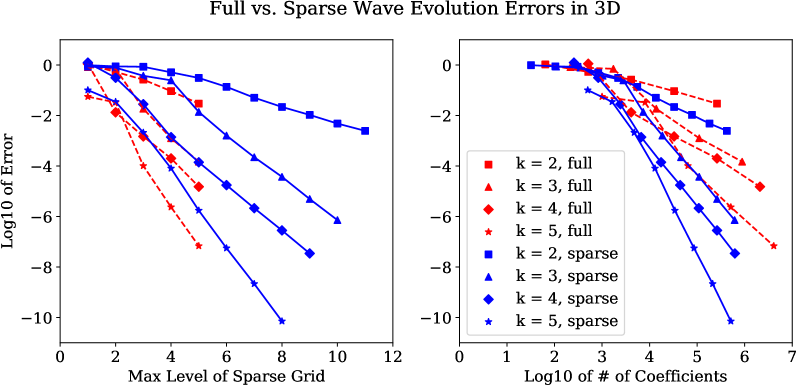
Figure 11: Comparison of full vs. sparse traveling wave evolution for 1.32 crossing times in 3D, using $\mathbf{k}=2\pi\cdot[1,2,-1]$ from $t=0$ to $t=0.54$ at various levels and polynomial degrees, with periodic boundary conditions.

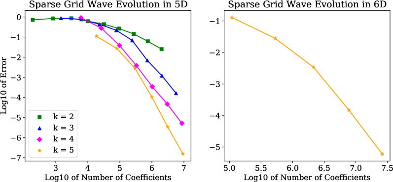
Figure 12: Error of traveling wave evolutions in 5 and 6 dimensions. Left: after $1.43$ crossing times in 5D, using $\mathbf{k}=2\pi\cdot[1,0,-1,2,1]$ from $t=0$ to $t=0.54$ for levels $1$ to $5$ at different polynomial degrees, with periodic boundary conditions. Right: after $1.52$ crossing times in 6D using $\mathbf{k}=2\pi\cdot[1,0,-1,2,1,-1]$ from $t=0$ to $t=0.54$ at $k=5$ for levels $1$ to $5$.

VII Conclusion

We review Sparse Grids as discretization method that breaks the curse of dimensionality. We develop a novel sparse grid discretization method using Operator-based Discontinuous Galerkin Finite Elements (OLDG), based on work by Guo and Cheng guo2016 and Wang et al. wang2016 . Particularly for higher-order methods, DGFE methods exhibit more locality than finite-differencing (FD) based methods: derivative operator matrices have a block-structured sparsity structure that is more efficient (cache friendly) on current computing architectures than the banded structure one finds in FD methods.

Our work is based on the prior works of Wang et al. wang2016 and Guo and Cheng guo2016 . We extend these prior works from elliptic and hyperbolic transport-type PDEs to hyperbolic wave-type PDEs by applying ideas from the OLDG method presented in miller2016 . This leads to a novel DG formulation for sparse grids that does not require a flux-conservative formulation of the PDEs. In particular, we define an explicit derivative operator in the sparse DG space that automatically takes the discontinuities at element boundaries into account, and leads to stable time evolutions (possibly requiring some artificial dissipation for non-linear systems).

We compare theoretical estimates and actual measurements for numerical accuracy vs. storage and run-time cost, and find that sparse grids are far superior in all cases we examine, including evolving the scalar wave equation in $3+1$, $5+1$, and $6+1$ dimensions. We are able to perform these calculation on a single workstation. On a full grid, the state vector for the highest-resolution $6$-D wave equation ($n=5,\,k=5$; see figure 12) would consume an estimated $268\,\mathrm{Terabyte}$ of storage for the state vector that would require a supercomputer.

We are optimistic that these accuracy improvements and cost reductions will survive contact with real-world applications that might include turbulence, shock waves, or highly anisotropic scenarios such as radiation transport. In how far this is indeed the case will be the topic of further research. Well-known numerical methods such as adaptive mesh refinement have been successfully applied to Sparse Grids bungartz2004sparse ; griebel1997 ; hegland2001 ; pfugler2010 , and should help mitigate issues encountered in real-world scenarios.

Another avenue that is described in the literature, but which we have not explored yet, is to choose a slightly different norm for our function space, for example the Sobolev space energy norm for $H^{1}_{0}$ as in bungartz2004sparse ; byrenheid2016 . This selects basis functions in a different order, and further reduces the cost from $O(N\log^{D-1}N)$ to $O(N)$. While this is already supported in principle by our software, we have not tested it. This sparse basis would induce a certain increase in complexity in managing basis functions, and the practical benefit of this method for relativistic astrophysics still needs to be demonstrated.

We anticipate that Sparse Grids will allow novel higher-dimensional studies in astrophysics and numerical relativity that are currently impossible to perform, or will at least significantly reduce the cost of such studies. This might be particularly relevant e.g. to radiation transfer in supernova calculations, to numerical investigations of black holes higher-dimensional ($D>3+1$) spacetimes, or to simply reduce the cost of high-resolution gravitational wave-form calculations in “standard” numerical relativity.

Appendix A Notation

Symbol	Meaning
$\mathbf{V}$	Function space to be discretized
$N$	total number of subintervals in the discretization
$D$	total dimension
$\phi$	Hat function on $[-1,1]$
$\ell$	Denoting a level in 1-D
$n$	Max level cutoff (all dimensions)
$i$	Cell number at a given level, referred to as the node
$\phi_{\ell,i}$	Shifted and scaled hat function $\phi$ to $i$th cell of level $\ell$
$\mathbf{V}_{n}$	Discretization of function space on 1D unit interval $[0,1]$ using hat functions up to level $n$
$\mathbf{W}_{\ell}$	Complement of $\mathbf{V}_{\ell-1}$ in $\mathbf{V}_{\ell}$ in terms of hat function basis
$\mathbf{l}$	$D$-tuple of levels (a multi-level)
$\phi_{\mathbf{l}}$	Tensor product of functions $\phi_{\mathbf{l}_{i}}(\mathbf{x}_{i})$
$\mathbf{V}_{\mathbf{l}}$	Tensor product of one-dimensional spaces $\mathbf{V}_{\mathbf{l}_{i}}$
$\mathbf{W}_{\mathbf{l}}$	Tensor product of one-dimensional spaces $\mathbf{W}_{\mathbf{l}_{i}}$
$\mathbf{V}_{n}^{D}$	Shorthand for $\mathbf{V}_{(n,n,\dots,n)}$: full grid space of hat functions up to level $n$ in $D$ dimensions
$\mathbf{\hat{V}}_{n}^{D}$	Sparse grid space of hat functions up to level $n$ in $D$ dimensions
$P$	Dimension of discretized space, AKA number of coefficients for a function representation
$k$	Dimension of space of polynomials on each cell of a DG basis.
$m$	Mode number in a given cell, running from $1$ to $k$
$h_{n,i,m}$	Basis function of the $m$th mode in the $i$th cell at level $n$
$v_{\ell,i,m}$	Hierarchical basis of DG functions
$\mathbf{V}_{n,k}$	Discretization of function space on 1D unit interval $[0,1]$ using a DG basis up to level $n$ and polynomial order $<\!k$
$\mathbf{W}_{n,k}$	Orthogonal complement of $\mathbf{V}_{n-1,k}$ in $\mathbf{V}_{n,k}$
$\mathbf{W}_{\mathbf{l},k}$	Tensor product of one-dimensional spaces $\mathbf{W}_{\mathbf{l}_{i}}$
$\mathbf{V}_{n,k}^{D}$	Shorthand for $\mathbf{W}_{(n,n,\dots,n),k}$: full grid space of DG functions up to level $n$, order $<\!k$ in $D$ dimensions
$\mathbf{\hat{V}}_{n,k}^{D}$	Sparse grid space of DG functions up to level $n$, order $<\!k$ in $D$ dimensions
$\mathcal{D}_{i,m;i^{\prime},m^{\prime}}$	Matrix element of 1-D derivative operator in position basis
$\mathcal{D}^{\text{hier}}$	Derivative operator in 1-D hierarchical basis
$\mathcal{D}^{\text{full}}_{a}$	Derivative operator in full basis along the $a$th axis
$\mathcal{D}^{\text{sparse}}_{a}$	Derivative operator in sparse basis along the $a$th axis

References

- [1] Richard Ernest Bellman. Dynamic Programming. Dover Publications, Incorporated, 2003.
- [2] Sergey A. Smolyak. Quadrature and interpolation formulas for tensor products of certain classes of functions. Dokl. Akad. Nauk SSSR, 4:240–243, 1963.
- [3] Hans-Joachim Bungartz and Michael Griebel. Sparse grids. Acta numerica, 13:147–269, 2004.
- [4] Thomas Gerstner and Michael Griebel. Sparse Grids. John Wiley & Sons, Ltd, 2010.
- [5] Wei Guo and Yingda Cheng. A sparse grid discontinuous galerkin method for high-dimensional transport equations and its application to kinetic simulations. SIAM Journal on Scientific Computing, 38(6):A3381–A3409, 2016.
- [6] Zixuan Wang, Qi Tang, Wei Guo, and Yingda Cheng. Sparse grid discontinuous galerkin methods for high-dimensional elliptic equations. J. Comput. Phys., 314(C):244–263, June 2016.
- [7] Jeff Bezanson, Alan Edelman, Stefan Karpinski, and Viral B. Shah. Julia: A fresh approach to numerical computing. SIAM Review, 59(1):65–98, 2017.
- [8] Christoph Zenger. Sparse Grids, volume 31. Friedrich Vieweg & Sohn Verlagsgesellschaft, 1991.
- [9] Joseph Traub and Henryk Wozniakowski. A General Theory of Optimal Algorithms. Academic Press, January 1980.
- [10] Jonah M Miller and Erik Schnetter. An operator-based local discontinuous galerkin method compatible with the bssn formulation of the einstein equations. Classical and Quantum Gravity, 34(1):015003, 2017.
- [11] Bradley K. Alpert. A class of bases in l2 for the sparse representations of integral operators. SIAM J. Math. Anal., 24(1):246–262, January 1993.
- [12] Schwab, Christoph, Süli, Endre, and Todor, Radu Alexandru. Sparse finite element approximation of high-dimensional transport-dominated diffusion problems. ESAIM: M2AN, 42(5):777–819, 2008.
- [13] Gary Cohen and Sebastien Pernet. Finite Element and Discontinuous Galerkin Methods for Transient Wave Equations. Springer, 2017.
- [14] Jan S. Hesthaven and Tim Warburton. Nodal Discontinuous Galerkin Methods: Algorithms, Analysis, and Applications. Springer Publishing Company, Incorporated, 1st edition, 2010.
- [15] Douglas N. Arnold, Franco Brezzi, Bernardo Cockburn, and Donatella Marini. Discontinuous Galerkin Methods for Elliptic Problems, pages 89–101. Springer Berlin Heidelberg, Berlin, Heidelberg, 2000.
- [16] ODE.jl. 2017-09-23. 0.7.0. https://github.com/JuliaDiffEq/ODE.jl.
- [17] M. Griebel. Adaptive sparse grid multilevel methods for elliptic pdes based on finite differences. Computing, 61(2):151–179, October 1998.
- [18] M. Hegland. Adaptive sparse grids. In ANZIAM J, pages 335–353, 2001.
- [19] Dirk Pflüger, Benjamin Peherstorfer, and Hans-Joachim Bungartz. Spatially adaptive sparse grids for high-dimensional data-driven problems. Journal of Complexity, 26(5):508 – 522, 2010. SI: HDA 2009.
- [20] Glenn Byrenheid, Dinh Dũng, Winfried Sickel, and Tino Ullrich. Sampling on energy-norm based sparse grids for the optimal recovery of Sobolev type functions in H. Journal of Approximation Theory, 207(Supplement C):207 – 231, 2016.