$H$-compactness of elliptic operators on weighted Riemannian Manifolds

Abstract.

In this paper we study the asymptotic behavior of second-order uniformly elliptic operators on weighted Riemannian manifolds. They naturally emerge when studying spectral properties of the Laplace-Beltrami operator on families of manifolds with rapidly oscillating metrics. We appeal to the notion of $H$-convergence introduced by Murat and Tartar. In our main result we establish an $H$-compactness result that applies to elliptic operators with measurable, uniformly elliptic coefficients on weighted Riemannian manifolds. We further discuss the special case of “locally periodic” coefficients and study the asymptotic spectral behavior of compact submanifolds of $\mathbb{R}\hskip 0.5pt^{n}$ with rapidly oscillating geometry.

1. Introduction

We study the asymptotic behavior of elliptic operators on families of weighted Riemannian manifolds that might feature fast oscillations. In this introduction we survey the results and the structure of this paper without going into detail. The precise definitions and statements can then be found in Section 2.

Convergence of metric measure spaces, in particular, Riemannian manifolds, has attracted an enormous amount of attention. Especially, substantial effort has been devoted to establishing geometric criteria for the convergence of spectral structures, e.g., see [6, 13, 14, 19, 17, 20, 18, 24, 22, 3, 8, 15].

Our point of view is different. We establish a compactness result that shows that any family of (uniformly elliptic) PDEs of the form $-{\mathop{\operatorname{div}}}_{g_{\varepsilon},\mu_{\varepsilon}}(\mathbb{L}_{\varepsilon}\nabla_{g_{\varepsilon}})u=f$ defined on a uniformly bi-Lipschitz diffeomorphic family of weighted Riemannian manifolds $(M_{\varepsilon},g_{\varepsilon},\mu_{\varepsilon})$ admits an $H$-convergent subsequence. The latter notion has been introduced in the context of homogenization of elliptic PDEs on $\mathbb{R}^{n}$ (in divergence form and of second-order), see [25]. In particular, in our setting it yields the existence of a limiting manifold and a limiting elliptic PDE such that solutions to the elliptic PDE on $M_{\varepsilon}$ converge as $\varepsilon\downarrow 0$ to the solution of the limiting PDE. Our approach in particular allows us to treat Riemannian manifolds which oscillate rapidly on a small length scale $0<\varepsilon\ll 1$.

This should be compared with the seminal work by Kuwae and Shioya [17], where spectral convergence is established for families of manifolds which are locally bi-Lipschitz diffeomorphic to a reference manifold with a bi-Lipschitz constant converging to $1$. In situations where the manifold features rapid oscillations, the family of diffeomorphisms between the manifolds is only uniformly bi-Lipschitz but not locally close to an isometry—and thus the approach in [17] is not applicable. In contrast, as we shall show, it is still possible to establish $H$-convergence, which in the symmetric case (e.g. when considering the Laplace-Beltrami operator on $M_{\varepsilon}$) implies Mosco-convergence of the associated energy forms, and the convergence of the associated spectrum. Moreover, our approach also applies to non-symmetric PDEs.

For general uniformly bi-Lipschitz diffeomorphic families of manifolds the limiting manifold and PDE depends on the extracted subsequence. However, under geometric conditions for $(M_{\varepsilon})$, we can uniquely identify the limit by appealing to suitable homogenization formulas (see Section 2.2). In the flat case, a natural geometric condition is periodicity of the coefficient field. In the case of PDEs on Riemannian manifolds with a symmetry structure, or for general manifolds that feature periodicity in local coordinates, we obtain similar identification results and homogenization formulas.

The latter might be of interest for applications to diffusion models in biomechanics, which is another motivation of our work. In this context, diffusion and reaction-diffusion processes in biological membranes and through interfaces are studied, e.g. see [1, 10, 30, 28]. One observation made is that “diffusion in biological membranes can appear anisotropic even though it is molecularly isotropic in all observed instances”, see [30]. We present examples (see below) where anisotropic diffusion on surfaces emerges on large scales from isotropic diffusion on surfaces with rapidly oscillating geometry.

Examples

Before stating our results in a general form, we illustrate our findings on the level of examples. In the following we present four examples. Each example considers a family of $2$-dimensional submanifolds $(M_{\varepsilon})$ in $\mathbb{R}\hskip 0.5pt^{3}$ given by an explicit formula and depending on a small parameter $\varepsilon>0$. In the limit $\varepsilon\downarrow 0$, $M_{\varepsilon}$ Hausdorff-converges (as a subset of $\mathbb{R}^{3}$) to a reference submanifold $M_{0}\subset\mathbb{R}^{3}$; however the spectrum of the associated Laplace-Beltrami operator on $M_{\varepsilon}$ does not converge to the spectrum of the one on $M_{0}$. Nevertheless, we can associate to $(M_{\varepsilon})$ a $2$-dimensional submanifold $N_{0}\subset\mathbb{R}\hskip 0.5pt^{3}$ that captures the asymptotic spectral behavior of $(M_{\varepsilon})$ in the limit $\varepsilon\downarrow 0$: The spectrum of the Laplace-Beltrami operator on $M_{\varepsilon}$ converges to the spectrum of the Laplace-Beltrami operator on $N_{0}$ in the sense of Lemma 19 below. Proofs and further details are presented in Section 3.

(a) A graphical surface with star-shaped corrugations.

For $R>0$ and a smooth, $2\pi$-periodic function $f\colon[0,\infty)\to\mathbb{R}$ we introduce the family $(M_{\varepsilon})$ of $2$-dimensional submanifolds of $\mathbb{R}^{3}$:

(1) $$M_{\varepsilon}:=\Big{\{}\begin{pmatrix}r\sin\theta\\ r\cos\theta\\ \varepsilon f(\tfrac{\theta}{\varepsilon})\end{pmatrix};r\in(0,R),\theta\in[0,2\pi)\Big{\}}.$$

In Figure 1 we present $M_{\varepsilon}$ for some values of $\varepsilon$ in the case $f=\sin^{2}$. As an application of our results we show that the spectrum of the Laplace-Beltrami operator on $M_{\varepsilon}$ converges to the spectrum of the Laplace-Beltrami operator on the submanifold

(2) $$N_{0}:=\Big{\{}\begin{pmatrix}\rho_{0}(r)\sin\theta\\ \rho_{0}(r)\cos\theta\\ \int_{0}^{r}\sqrt{1-\rho_{0}^{\prime}(t)^{2}}\,\mathrm{d}t\end{pmatrix};r\in(0,R),\theta\in[0,2\pi)\Big{\}},$$

where $\rho_{0}(r)=\tfrac{1}{2\pi}\int_{0}^{2\pi}\sqrt{f^{\prime}(y)^{2}+r^{2}}\,\mathrm{d}y$, see Figure 1.

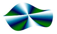
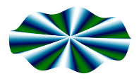
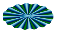
$\xrightarrow{\varepsilon\downarrow 0}$

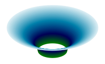
$\varepsilon=\tfrac{1}{2}$

$\varepsilon=\tfrac{1}{4}$

$\varepsilon=\tfrac{1}{8}$

Figure 1. A family of graphical surfaces with star-shaped corrugations. The three pictures on the left show $M_{\varepsilon}$ defined by (1) with $f=\sin^{2}$ and decreasing values of $\varepsilon$. The picture on the right shows the limiting surface $N_{0}$ defined via (2). As $\varepsilon\to 0$ the spectrum of the Laplace-Beltrami operator on $M_{\varepsilon}$ converges to the spectrum of the Laplace-Beltrami operator on $N_{0}$. The color indicates the height component.

(b) A carambola-shaped sphere in $\mathbb{R}\hskip 0.5pt^{3}$.

We can transfer the example above from a graph over $\mathbb{R}^{2}$ to a sphere with oscillatory perturbation of its radius as depicted in Figure 2. More precisely, for a smooth $2\pi$-periodic function $f\colon[0,\infty)\to\mathbb{R}$ we consider the family $(M_{\varepsilon})$ of $2$-dimensional submanifolds of $\mathbb{R}^{3}$:

(3) $$M_{\varepsilon}:=\Big{\{}(1+\varepsilon f(\tfrac{\theta}{\varepsilon}))\begin{pmatrix}\sin\varphi\sin\theta\\ \sin\varphi\cos\theta\\ \cos\varphi\end{pmatrix};\varphi\in(0,\pi),\theta\in[0,2\pi)\Big{\}}.$$

In that case a limiting submanifold is given by

(4) $$N_{0}:=\Big{\{}\begin{pmatrix}\rho_{0}(\varphi)\sin\theta\\ \rho_{0}(\varphi)\cos\theta\\ \int_{0}^{\varphi}\sqrt{1-\rho_{0}^{\prime}(t)^{2}}\,\mathrm{d}t\end{pmatrix};\varphi\in(0,\pi),\theta\in[0,2\pi)\Big{\}},$$

where $\rho_{0}(\varphi)=\tfrac{1}{2\pi}\int_{0}^{2\pi}\sqrt{f^{\prime}(y)^{2}+\sin^{2}\varphi}\,\mathrm{d}y$. See Figure 2 for a visualization in the case $f=\sin^{2}$.

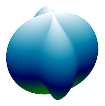
$\xrightarrow{\varepsilon\downarrow 0}$

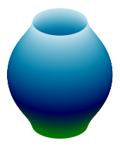
$\varepsilon=\tfrac{1}{2}$

$\varepsilon=\tfrac{1}{4}$

$\varepsilon=\tfrac{1}{8}$

Figure 2. A family of spheres with radial perturbations oscillating with the longitude. The three pictures on the left show $M_{\varepsilon}$ defined by (3) with $f=\sin^{2}$ and decreasing values of $\varepsilon$. The picture on the right shows the limiting surface $N_{0}$ defined via (4).

(c) A corrugated, rotationally symmetric submanifold in $\mathbb{R}\hskip 0.5pt^{3}$.

In contrast to the previous example we assume a sphere with radial perturbations with the latitude, i.e. for a smooth $\pi$-periodic function $f\colon[0,\infty)\to\mathbb{R}$ we consider the family $(M_{\varepsilon})$ of $2$-dimensional submanifolds of $\mathbb{R}^{3}$:

(5) $$M_{\varepsilon}:=\Big{\{}(1+\varepsilon f(\tfrac{\varphi}{\varepsilon})\begin{pmatrix}\sin\varphi\sin\theta\\ \sin\varphi\cos\theta\\ \cos\varphi\end{pmatrix};\varphi\in(0,\pi),\theta\in[0,2\pi)\Big{\}}.$$

In that case a limiting submanifold is given by

(6) $$N_{0}:=\Big{\{}\begin{pmatrix}\sin\varphi\sin\theta\\ \sin\varphi\cos\theta\\ \int_{0}^{\varphi}\sqrt{\tfrac{\rho_{0}(t)^{2}}{\sin^{2}t}-\cos^{2}t}\,\mathrm{d}t\end{pmatrix};\varphi\in(0,\pi),\theta\in[0,2\pi)\Big{\}},$$

where $\rho_{0}(\varphi)=\tfrac{\sin\varphi}{\pi}\int_{0}^{\pi}\sqrt{f^{\prime}(y)^{2}+1}\,\mathrm{d}y$. See Figure 3 for the case $f=\sin^{2}$.

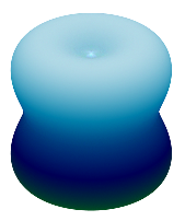
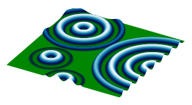
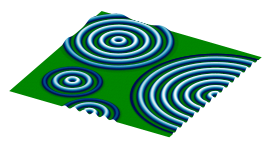
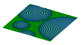
$\xrightarrow{\varepsilon\downarrow 0}$

$\varepsilon=\tfrac{1}{2}$

$\varepsilon=\tfrac{1}{4}$

$\varepsilon=\tfrac{1}{8}$

Figure 3. A family of spheres with radial perturbations oscillating with the latitude. The three pictures on the left show $M_{\varepsilon}$ defined by (5) with $f=\sin^{2}$ and decreasing values of $\varepsilon$. The picture on the right shows the limiting surface $N_{0}$ defined via (6).

(d) A locally corrugated graphical surface.

Consider a relatively-compact open set $Y\subset\mathbb{R}^{2}$ and a set $Z\in Y$ of isolated points. For every point $z\in Z$ we use a smooth function $\psi_{z}\colon[0,\infty)\to[0,1]$ to define a rotationally symmetric cut-off function $\psi_{z}(|\cdot-z|)$ such that

$$\begin{cases}\text{$\psi_{z}(0)=1$,}&\\ \text{$\mathrm{supp}\psi_{z}(|\cdot-z|)\cap\mathrm{supp}\psi_{z^{\prime}}(|\cdot-z^{\prime}|)=\emptyset$ for all $z^{\prime}\in Z\setminus\{z\}$.}\end{cases}$$

Now we consider a smooth $T$-periodic function $f\colon[0,\infty)\to\mathbb{R}$ and the set $M_{\varepsilon}$ which is the graph of the function

(7) $$Y\setminus Z\ni x\mapsto\sum_{z\in Z}\varepsilon f\big{(}\tfrac{|x-z|}{\varepsilon}\big{)}\psi_{z}(|x-z|)\in\mathbb{R}^{3},$$

which we regard as a two-dimensional submanifold of $\mathbb{R}\hskip 0.5pt^{3}$. In that case a limiting submanifold is given by

(8) $$Y\setminus Z\ni x\mapsto\sum_{z\in Z}\int_{0}^{|x-z|}\sqrt{\tfrac{\rho_{0,z}(t)^{2}}{t^{2}}-1}\,\mathrm{d}t\in\mathbb{R}^{3},$$

where $\rho_{0,z}(r)=\tfrac{r}{T}\int_{0}^{T}\sqrt{f^{\prime}(y)^{2}\psi_{z}(r)^{2}+1}\,\mathrm{d}y$. See Figure 4 for the case $f=\sin^{2}$.

$\xrightarrow{\varepsilon\downarrow 0}$

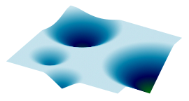
$\varepsilon=\tfrac{1}{2}$

$\varepsilon=\tfrac{1}{4}$

$\varepsilon=\tfrac{1}{8}$

Figure 4. A family of locally corrugated graphical surfaces. The three pictures on the left show $M_{\varepsilon}$ defined via (7) with $f=\sin^{2}$ and decreasing values of $\varepsilon$. The picture on the right shows the limiting surface $N_{0}$ defined via (8).

General setting and the structure of the paper

Throughout this paper we consider weighted Riemannian manifolds $M=(M,g,\mu)$ with metric $g$ and measure $\mu$. We always assume that $M$ is $n$-dimensional (with $n\geq 2$), smooth, connected, without boundary, and that $\mu$ has a smooth positive density against the Riemannian volume associated with $g$. We refer to the end of the introduction for a summary of standard notation that we use in this paper. The examples discussed above belong to the following general setting:

Definition 1 (Uniformly bi-Lipschitz diffeomorphic families of manifolds).

A family of weighted Riemannian manifolds $(M_{\varepsilon},g_{\varepsilon},\mu_{\varepsilon})$ indexed by $0<\varepsilon<1$ is called uniformly bi-Lipschitz diffeomorphic, if there exits a weighted Riemannian manifold $(M_{0},g_{0},\mu_{0})$ and a constant $C$ such that for all $\varepsilon$ there exist diffeomorphisms $h_{\varepsilon}\colon M_{0}\to M_{\varepsilon}$ with

(9) $$\tfrac{1}{C}|\xi|\leq|dh_{\varepsilon}(x)\xi|\leq C|\xi|\qquad\text{for all $x\in M_{0}$ and $\xi\in T_{x}M_{0}$}.$$

We call $(M_{0},g_{0},\mu_{0})$ reference manifold.

In the setting of (9) the Laplace-Beltrami operator on $M_{\varepsilon}$ gives rise to a second-order elliptic operator ${\mathop{\operatorname{div}}}(\mathbb{L}_{\varepsilon}\nabla)$ on $M_{0}$ with a uniformly elliptic coefficient field $\mathbb{L}_{\varepsilon}$, i.e.

$$g_{0}(\xi,\mathbb{L}_{\varepsilon}\xi)\geq\tfrac{1}{C^{n+2}}|\xi|^{2},\qquad g_{0}(\xi,\mathbb{L}_{\varepsilon}^{-1}\xi)\geq{C^{n+2}}|\xi|^{2}\qquad\text{for every $\xi\in TM_{0}$},$$

see Section 2.3 for further details. It is therefore natural to consider homogenization of elliptic operators on the reference manifold with oscillating coefficients and measure. This is done in Section 2, where our results are presented.

Our main result, cf. Theorem 4, is a compactness result for $H$-convergence. In the symmetric case (e.g., for the Laplace-Beltrami operator) $H$-convergence implies Mosco-convergence of the associated energy forms, cf. Lemma 8, and the convergence of the spectrum of the associated second-order elliptic operators $-{\mathop{\operatorname{div}}}(\mathbb{L}_{\varepsilon}\nabla)$, cf. Lemma 10. In Section 2.2 we address the problem of identifying the limiting PDE and manifold. In particular, we provide a homogenization formula for manifolds that feature periodicity in local coordinates. In Section 2.3 we discuss the application to families of parametrized manifolds that are bi-Lipschitz diffeomorphic. In particular, for such families, we establish spectral convergence (along subsequences) in Lemma 19 and discuss the special case of families of submanifolds of $\mathbb{R}\hskip 0.5pt^{d}$, see Lemma 20. In Section 3 we discuss concrete examples as the ones presented above. All proofs of the results in this paper are presented in Section 4.

Notation. For the background of the analysis on manifolds, we refer the readers to [7, 12].

• Let $\Omega\subset M$ open. We write $\omega\Subset\Omega$ if $\omega$ is an open set such that the closure $\overline{\omega}$ is compact and $\overline{\omega}\subset\Omega$.

• We use $h$ for a diffeomorphism between manifolds and denote its differential by $dh$. We use $\mathbb{L}$ for a measurable $(1,1)$-tensor field on a manifold. We call $\mathbb{L}$ also a coefficient field on the manifold.

• We use the notation $(\cdot,\cdot)(x)=g(\cdot,\cdot)(x)$ and $|\xi|(x)=\sqrt{g(\xi,\xi)(x)}$ to denote the inner product and induced norm in $T_{x}M$ at $x\in M$. We tacitly simply write $(\xi,\eta)$ and $|\xi|$ instead of $(\xi,\eta)(x)$ and $|\xi|(x)$ if the meaning is clear from the context.

• For a (sufficiently regular) function $u$ and vector field $\xi$ on $\Omega$, the gradient of $u$ is denoted by $\nabla_{g}u$ and the divergence of $\xi$ is denoted by ${\mathop{\operatorname{div}}}_{g,\mu}\xi$, i.e., we have $g(\nabla_{g}u,\xi)=\xi u=du(\xi)$ and $-\int_{\Omega}g({\mathop{\operatorname{div}}}_{g,\mu}\xi,u)\,\mathrm{d}\mu=-\int_{\Omega}g(\xi,\nabla_{g}u)\,\mathrm{d}\mu$ provided either $u$ or $\xi$ are compactly supported. In particular, we write $\triangle_{g,\mu}:={\mathop{\operatorname{div}}}_{g,\mu}\nabla_{g}$ to denote the (weighted) Laplace-Beltrami operator. If the meaning is clear from the context, we shall simply write $\nabla,{\mathop{\operatorname{div}}}$, and $\Delta$. In some situations the Riemannian manifold will be parametrized by the parameter $\varepsilon$; in that case, we may us the notation $\nabla_{\varepsilon},{\mathop{\operatorname{div}}}_{\varepsilon}$ and $\triangle_{\varepsilon}$. If there is no danger of confusion, we may drop the index $\varepsilon$ in the notation.

• For $\Omega\subset M$ open we denote by $L^{2}(\Omega,g,\mu)$ the Hilbert space of square integrable functions and denote by

  $$\|u\|_{L^{2}(\Omega,g,\mu)}^{2}:=\int_{\Omega}|u|^{2}\,\mathrm{d}\mu$$

  the associated norm. We denote by $L^{2}(T\Omega)$ the space of measurable sections $\xi$ of $T\Omega$ such that $|\xi|\in L^{2}(\Omega,g,\mu)$.

• We denote by $C^{\infty}_{c}(\Omega)$ the space of smooth compactly supported functions, and by $H^{1}(\Omega,g,\mu)$ the usual Sobolev space on $(\Omega,g,\mu)$, i.e. the space of functions $u\in L^{2}(\Omega,g,\mu)$ with distributional first derivatives in $L^{2}(\Omega,g,\mu)$. Equipped with the norm

  $$\|u\|_{H^{1}(\Omega,g,\mu)}^{2}:=\int_{M}|u|^{2}+|\nabla u|^{2}\,\mathrm{d}\mu$$

  (and the usual inner product), $H^{1}(\Omega,g,\mu)$ is a Hilbert space.

• We denote by $H_{0}^{1}(\Omega,g,\mu)$ the closure of $C^{\infty}_{c}(\Omega)$ in $H^{1}(\Omega,g,\mu)$. We denote by $H^{-1}(\Omega,g,\mu)$ the dual space to $H^{1}_{0}(\Omega,g,\mu)$ and use the notation $\langle F,u\rangle_{(\Omega,g,\mu)}$ to denote the dual pairing of $F\in H^{-1}(\Omega,g,\mu)$ and $u\in H^{1}_{0}(M,g,\mu)$.

We tacitly simply write $\Omega$ (instead of $(\Omega,g,\mu)$), $L^{2}(\Omega)$, $H^{1}(\Omega)$, $\|\cdot\|_{L^{2}(\Omega)}$, $\|\cdot\|_{H^{1}(\Omega)}$, $\langle\cdot,\cdot\rangle$, if the meaning is clear from the context.

2. Statement of the main results

2.1. H-, Mosco- and spectral convergence

We are interested in second-order elliptic operators of the form

$$-{\mathop{\operatorname{div}}}(\mathbb{L}\nabla)\colon H^{1}_{0}(\Omega)\to H^{-1}(\Omega),\qquad\Omega\subset M\text{ open},$$

where $-{\mathop{\operatorname{div}}}=-{\mathop{\operatorname{div}}}_{g,\mu}\colon L^{2}(T\Omega)\to H^{-1}(\Omega)$ is the adjoint of $\nabla=\nabla_{g}\colon H^{1}_{0}(\Omega)\to L^{2}(T\Omega)$, and $\mathbb{L}$ denotes a uniformly elliptic coefficient field defined on $\Omega$. More precisely, for $0<\lambda\leq\Lambda$ and $\Omega\subset M$ open, we denote by $\mathcal{M}(\Omega,\lambda,\Lambda)$ the set of all measurable coefficient fields $\mathbb{L}\colon\Omega\to\operatorname{Lin}(T\Omega)$ that are uniformly elliptic and bounded in the sense that for $\mu$-a.e. $x\in\Omega$ and all $\xi\in T_{x}\Omega$

(10) $$g(\xi,\mathbb{L}(x)\xi) \geq\lambda|\xi|^{2},$$

(11) $$g(\xi,(\mathbb{L}(x))^{-1}\xi) \geq\tfrac{1}{\Lambda}|\xi|^{2}.$$

Moreover, we denote by $m_{0}(\Omega)$ the infimum of all $m\in\mathbb{R}\hskip 0.5pt$ such that

$$\inf\Big{\{}\int_{\Omega}m|u|^{2}+g(\nabla u,\nabla u)\,\mathrm{d}\mu;u\in H^{1}_{0}(\Omega)\text{ with }\|u\|_{H^{1}_{0}(\Omega)}=1\Big{\}}>0.$$

(See Remark 2 below for a discussion of $m_{0}(\Omega)$). Given a family $(\mathbb{L}_{\varepsilon})_{\varepsilon>0}\subset\mathcal{M}(\Omega,\lambda,\Lambda)$ and $f\in H^{-1}(\Omega)$ we study the asymptotic behavior as $\varepsilon\downarrow 0$ of the solution $u_{\varepsilon}\in H^{1}_{0}(\Omega)$ to the equation

(12) $$mu_{\varepsilon}-{\mathop{\operatorname{div}}}(\mathbb{L}_{\varepsilon}\nabla u_{\varepsilon})=f\qquad\text{ in }H^{-1}(\Omega),$$

where $m$ denotes a fixed scalar satisfying $m>\frac{m_{0}(\Omega)}{\lambda}$.

Remark 2.

By the Lax-Milgram lemma, (12) admits a unique solution $u_{\varepsilon}\in H^{1}_{0}(\Omega)$ satisfying

(13) $$\|u_{\varepsilon}\|_{H^{1}(\Omega)}\leq C(\Omega,\lambda,m)\|f\|_{H^{-1}(\Omega)}.$$

We briefly comment on the constant $m_{0}(\Omega)$, which appears in the lower bound condition for $m$ in (12). If $\Omega\Subset M$ is relatively-compact and connected, then Poincaré’s inequality (for functions with zero mean) holds:

$$\forall u\in H^{1}(\Omega)\,:\qquad\int_{\Omega}\Big{|}u-\tfrac{1}{\mu(\Omega)}\int_{\Omega}u\,\,\mathrm{d}\mu\Big{|}^{2}\,\,\mathrm{d}\mu\leq C_{\Omega}\int_{\Omega}|\nabla u|^{2}\,\,\mathrm{d}\mu.$$

In this case we have $m_{0}(\Omega)\leq 0$, and in (12) any $m>0$ is admissible. Also note that, the condition $m_{0}(\Omega)<0$ is equivalent to the validity of Poincare’s inequality (for functions with vanishing boundary conditions):

(14) $$\forall u\in H^{1}_{0}(\Omega)\,:\qquad\int_{\Omega}|u|^{2}\,\,\mathrm{d}\mu\leq C^{\prime}_{\Omega}\int_{\Omega}|\nabla u|^{2}\,\,\mathrm{d}\mu,$$

where $C^{\prime}_{\Omega}>0$ denotes a generic constant (only depending on $n$). Moreover, if $m_{0}(\Omega)<0$, then in (12) we may then consider the case $m=0$.

H-compactness

Our first main result is a compactness result concerning the homogenization limit $\varepsilon\downarrow 0$. It relies on the notion of $H$-convergence which goes back to the seminal work by Murat and Tartar ([25]) where the notion is introduced in the flat case $M=\mathbb{R}\hskip 0.5pt^{n}$. It is a generalization of the notion of $G$-convergence by Spagnolo and De Giorgi. The definition of $H$-convergence can be phrased in our setting as follows:

Definition 3 ($H$-convergence).

Let $\Omega\subset M$ be open. We say a sequence $(\mathbb{L}_{\varepsilon})\subset\mathcal{M}(\Omega,\lambda,\Lambda)$ $H$-converges in $(\Omega,g,\mu)$ to $\mathbb{L}_{0}\in\mathcal{M}(\Omega,\lambda,\Lambda)$ as $\varepsilon\to 0$, if for any relatively-compact open subset $\omega\Subset\Omega$ with $m_{0}(\omega)<0$, and any $f\in H^{-1}(\omega)$, the unique solutions $u_{\varepsilon},u_{0}\in H^{1}_{0}(\omega)$ to

$$-{\mathop{\operatorname{div}}}(\mathbb{L}_{\varepsilon}\nabla u_{\varepsilon})=-{\mathop{\operatorname{div}}}(\mathbb{L}_{0}\nabla u_{0})=f\qquad\text{in }H^{-1}(\omega)$$

satisfy

$$\begin{cases}u_{\varepsilon}\rightharpoonup u_{0}&\quad\text{weakly in }H^{1}(\omega),\\ \mathbb{L}_{\varepsilon}\nabla u_{\varepsilon}\rightharpoonup\mathbb{L}_{0}\nabla u_{0}&\quad\text{weakly in }L^{2}(T\omega).\end{cases}$$

In that case we write $\mathbb{L}_{\varepsilon}\stackrel{{\scriptstyle H}}{{\to}}\mathbb{L}_{0}$ in $(\Omega,\mu,g)$ as $\varepsilon\to 0$.

Our main result is the following $H$-compactness statement:

Theorem 4.

Let $\lambda,\Lambda>0$ and let $(\mathbb{L}_{\varepsilon})$ denote a sequence in $\mathcal{M}(M,\lambda,\Lambda)$. Then there exist a subsequence (not relabeled) and $\mathbb{L}_{0}\in\mathcal{M}(M,\lambda,\Lambda)$ such that the following holds:

1. $\mathbb{L}_{\varepsilon}\stackrel{{\scriptstyle H}}{{\to}}\mathbb{L}_{0}$ in $(M,g,\mu)$.

2. For every $\Omega\subset M$ open, every $m>\frac{m_{0}(\Omega)}{\lambda}$, and sequences $(f_{\varepsilon})\subset L^{2}(\Omega)$ and $(F_{\varepsilon})\subset L^{2}(T\Omega)$ with

   $$\begin{cases}f_{\varepsilon}\rightharpoonup f_{0}&\quad\text{weakly in }L^{2}(\Omega),\\ F_{\varepsilon}\to F_{0}&\quad\text{in }L^{2}(T\Omega),\end{cases}$$

   the solutions $u_{\varepsilon},u_{0}\in H^{1}_{0}(\Omega)$ to

   (15) $$mu_{\varepsilon}-{\mathop{\operatorname{div}}}(\mathbb{L}_{\varepsilon}\nabla u_{\varepsilon})=f_{\varepsilon}+{\mathop{\operatorname{div}}}F_{\varepsilon} \quad\text{in }H^{-1}(\Omega),$$

   $$mu_{0}-{\mathop{\operatorname{div}}}(\mathbb{L}_{0}\nabla u_{0})=f_{0}+{\mathop{\operatorname{div}}}F_{0} \quad\text{in }H^{-1}(\Omega),$$

   satisfy

   $$\begin{cases}u_{\varepsilon}\rightharpoonup u_{0}&\quad\text{weakly in }H^{1}_{0}(\Omega),\\ \mathbb{L}_{\varepsilon}\nabla u_{\varepsilon}\rightharpoonup\mathbb{L}_{0}\nabla u_{0}&\quad\text{weakly in }L^{2}(T\Omega).\end{cases}$$

   Additionally we have $u_{\varepsilon}\to u_{0}$ strongly in $L^{2}(\Omega)$, if either $H^{1}_{0}(\Omega)$ is compactly embedded in $L^{2}(\Omega)$, or $m\neq 0$ and $f_{\varepsilon}\to f_{0}$ strongly in $L^{2}(\Omega)$.

For the proof see Section 4.2. The theorem is an extension of a classical result in [25] where (scalar) elliptic operators of the form $-\mbox{div}(A_{\varepsilon}\nabla)$ on $\mathbb{R}\hskip 0.5pt^{n}$ are considered. It has been extended to a large class of elliptic equations on $\mathbb{R}\hskip 0.5pt^{n}$ including e.g. linear elasticity [4] and monotone operators for vector valued fields ([5]). See also [31] for a variant that applies to non-local operators.

In the following we briefly comment on the proof of Theorem 4, which is based on Murat and Tartar’s method of oscillating test-functions. In contrast to the classical flat case $M=\mathbb{R}\hskip 0.5pt^{n}$, we require a localization argument, since the tangent spaces $T_{x}M$ change when $x$ varies in $M$. We therefore first establish $H$-compactness restricted to sufficiently small balls $B$ (see Proposition 5 below) and then argue by covering $M$ with countably many of such balls.

Proposition 5 ($H$-compactness on small balls).

Let $(\mathbb{L}_{\varepsilon})\subset\mathcal{M}(M,\lambda,\Lambda)$ and let $B\Subset M$ denote an open ball with radius smaller than the injectivity radius at its center. Then there exits $\mathbb{L}_{0}\in\mathcal{M}(\tfrac{1}{2}B,\lambda,\Lambda)$ and a (not relabeled) subsequence of $(\mathbb{L}_{\varepsilon})$ such that $\mathbb{L}_{\varepsilon}\stackrel{{\scriptstyle H}}{{\to}}\mathbb{L}_{0}$ in $\frac{1}{2}B$, which is the open ball with the same center point and half the radius of $B$.

To lift Proposition 5 from small balls to the whole manifold we cover $M$ by a countable collection of sufficiently small balls and pass to a diagonal sequence that features $H$-convergence on each of these balls. In order to guarantee that the $H$-limits associated with these balls are identical on the intersections of the balls, we appeal to the following lemma, which in particular establishes the uniqueness and locality property of $H$-convergence:

Lemma 6 (Uniqueness, locality, invariance w.r.t. transposition).

Let $\Omega\subset M$ be open and consider a sequences $(\mathbb{L}_{\varepsilon})\subset\mathcal{M}(\Omega,\lambda,\Lambda)$ that $H$-converges to some $\mathbb{L}_{0}$ in $\Omega$.

1. Let $(\widetilde{\mathbb{L}}_{\varepsilon})\subset\mathcal{M}(\Omega,\lambda,\Lambda)$ denote another sequence that $H$-converges to some $\widetilde{\mathbb{L}}_{0}$ in $\Omega$. Suppose that for some open $\omega\Subset\Omega$ we have $\mathbb{L}_{\varepsilon}=\widetilde{\mathbb{L}}_{\varepsilon}$ in $\omega$ for all $\varepsilon$. Then $\mathbb{L}_{0}=\widetilde{\mathbb{L}}_{0}$ $\mu$-a.e. in $\omega$.

2. Consider the coefficient field $\mathbb{L}_{\varepsilon}^{*}$ defined by the identity

   $$g(\mathbb{L}_{\varepsilon}^{*}\xi,\eta)=g(\xi,\mathbb{L}_{\varepsilon}\eta)\qquad\text{for all }\xi,\eta\in T\Omega,$$

   i.e., the adjoint of $\mathbb{L}_{\varepsilon}$. Then $(\mathbb{L}_{\varepsilon}^{*})$ $H$-converges in $\Omega$ to $\mathbb{L}_{0}^{*}$ (the adjoint of $\mathbb{L}_{0}$).

Finally, to prove that $H$-convergence on the individual balls yields $H$-convergence on the entire manifold, and in order to treat the varying right-hand sides in part (b) of Theorem 4, we apply the following lemma.

Lemma 7.

Let $\Omega\subset M$ be open and $\mathbb{L}_{\varepsilon}\stackrel{{\scriptstyle H}}{{\to}}\mathbb{L}_{0}$ in $\Omega$. Let $\omega\Subset\Omega$ with $m_{0}(\omega)<0$. Then for every $f_{\varepsilon},f_{0}\in L^{2}(\omega)$ and $G_{\varepsilon},F_{\varepsilon},G_{0},F_{0}\in L^{2}(T\omega)$ with

$$\begin{cases}f_{\varepsilon}\rightharpoonup f_{0}&\quad\text{weakly in }L^{2}(\omega),\\ G_{\varepsilon}\to G_{0}&\quad\text{in }L^{2}(T\omega),\\ F_{\varepsilon}\to F_{0}&\quad\text{in }L^{2}(T\omega),\end{cases}$$

the unique solutions $u_{\varepsilon},u_{0}\in H^{1}_{0}(\omega)$ to

$$-{\mathop{\operatorname{div}}}(\mathbb{L}_{\varepsilon}\nabla u_{\varepsilon})=f_{\varepsilon}-{\mathop{\operatorname{div}}}(\mathbb{L}_{\varepsilon}G_{\varepsilon})-{\mathop{\operatorname{div}}}F_{\varepsilon} \quad\text{in }H^{-1}(\omega),$$

$$-{\mathop{\operatorname{div}}}(\mathbb{L}_{0}\nabla u_{0})=f_{0}-{\mathop{\operatorname{div}}}(\mathbb{L}_{0}G_{0})-{\mathop{\operatorname{div}}}F_{\varepsilon} \quad\text{in }H^{-1}(\omega)$$

satisfy

$$\begin{cases}u_{\varepsilon}\rightharpoonup u_{0}&\quad\text{weakly in }H^{1}_{0}(\omega),\\ \mathbb{L}_{\varepsilon}\nabla u_{\varepsilon}\rightharpoonup\mathbb{L}_{0}\nabla u_{0}&\quad\text{weakly in }L^{2}(T\omega).\end{cases}$$

Mosco-convergence and convergence of the spectrum

If we restrict to the symmetric case, i.e. $\mathbb{L}_{\varepsilon}$ satisfies

$$g(\mathbb{L}_{\varepsilon}\xi,\eta)=g(\xi,\mathbb{L}_{\varepsilon}\eta)\qquad\text{for all }\xi,\eta\in TM,$$

the solutions to (15) can be characterized as the unique minimizers in $H^{1}_{0}(\Omega)$ to the strictly convex and coercive functional

$$H^{1}_{0}(\Omega)\ni u\mapsto\mathcal{E}_{m,\varepsilon}(u)-\int_{M}f_{\varepsilon}u+g(F_{\varepsilon},\nabla u)\,\,\mathrm{d}\mu,$$

where

$$\mathcal{E}_{m,\varepsilon}(u):=\tfrac{1}{2}\int_{\Omega}m|u|^{2}+g(\mathbb{L}_{\varepsilon}\nabla u,\nabla u)\,\,\mathrm{d}\mu.$$

In this symmetric situation we can appeal to variational notions of convergence, in particular $\Gamma$-convergence and Mosco-convergence. The latter is extensively used to study the convergence properties of the associated evolution (i.e. the semigroup generated by $-{\mathop{\operatorname{div}}}(\mathbb{L}_{\varepsilon}\nabla)$), e.g. see [17, 19, 16, 22, 21]. See a work by Hino ([9]) for a non-symmetric generalization of Mosco-convergence. A simple argument (that we outline for the reader’s convenience—together with the definition of Mosco-convergence—in the appendix) shows that $H$-convergence implies Mosco-convergence (resp. Resolvent convergence):

Lemma 8 ($H$-convergence implies Mosco-convergence).

Let $\mathbb{L}_{\varepsilon}\in\mathcal{M}(M,\lambda,\Lambda)$ be symmetric. Suppose $\mathbb{L}_{\varepsilon}\stackrel{{\scriptstyle H}}{{\to}}\mathbb{L}_{0}$, then the functional $\mathcal{E}_{\varepsilon}\colon L^{2}(M)\to\mathbb{R}\hskip 0.5pt\cup\{+\infty\}$,

$$\mathcal{E}_{\varepsilon}(u)=\begin{cases}\int_{M}(\mathbb{L}_{\varepsilon}\nabla u,\nabla u)\,\mathrm{d}\mu&\quad u\in H^{1}_{0}(M),\\ \infty&\quad\mbox{otherwise}\end{cases}$$

Mosco-converges to $\mathcal{E}_{0}\colon L^{2}(M)\to\mathbb{R}\hskip 0.5pt\cup\{+\infty\}$,

$$\mathcal{E}_{0}(u)=\begin{cases}\int_{M}(\mathbb{L}_{0}\nabla u,\nabla u)\,\mathrm{d}\mu&\quad u\in H^{1}_{0}(M),\\ \infty&\quad\mbox{otherwise}.\end{cases}$$

Remark 9.

The notion of Mosco-convergence only directly yields strong convergence of $(u_{\varepsilon})$ in $L^{2}(M)$ (and weak convergence in $H^{1}(M)$). The notion of $H$-convergence is a bit stronger, since it also yields convergence of the fluxes $\mathbb{L}_{\varepsilon}\nabla u_{\varepsilon}$. In contrast, Mosco-convergence in conjunction with the Div-Curl Lemma, see Lemma 24 below, only yields convergence of the $L^{2}$-projection of $\mathbb{L}_{\varepsilon}\nabla u_{\varepsilon}$ onto the orthogonal complement of $\{\nabla\phi\,:\,\phi\in H^{1}_{0}(M)\}\subset L^{2}(T\Omega)$.

Another consequence of $H$-convergence is convergence of the spectrum. In the following we consider an open, relatively-compact subset $\Omega\Subset M$ and suppose that $m_{0}(\Omega)<0$, so that Poincaré’s inequality (14) is available and the embedding $H^{1}_{0}(\Omega)\subset L^{2}(\Omega)$ is compact. Moreover, we consider a symmetric, uniformly elliptic coefficient field $\mathbb{L}_{\varepsilon}\in\mathcal{M}(M,\lambda,\Lambda)$. Then the spectral theorem for compact, self-adjoint operators applied to the operator $-{\mathop{\operatorname{div}}}(\mathbb{L}_{\varepsilon}\nabla):H^{1}_{0}(\Omega)\subset L^{2}(\Omega)\to L^{2}(\Omega)$ implies that $L^{2}(\Omega)$ decomposes into countably many, finite dimensional, orthogonal eigenspaces associated with strictly positive eigenvalues. The following statement shows that if $\mathbb{L}_{\varepsilon}$ is $H$-convergent, then the eigenspaces and eigenvalues converge. The statement is a direct consequence of [11, Lemma 11.3 and Theorem 11.5, see also Theorem 11.6] combined with Theorem 4:

Lemma 10 ($H$-convergence implies spectral convergence).

Let $(\mathbb{L}_{\varepsilon})$ be a sequence of symmetric coefficient fields in $\mathcal{M}(M,\lambda,\Lambda)$ and suppose that $\mathbb{L}_{\varepsilon}\stackrel{{\scriptstyle H}}{{\to}}\mathbb{L}_{0}$. Consider an open, relatively-compact set $\Omega\subset M$ with $m_{0}(\Omega)<0$. For $\varepsilon\geq 0$ we consider the unbounded operator

$$-{\mathop{\operatorname{div}}}(\mathbb{L}_{\varepsilon}\nabla):H^{1}_{0}(\Omega)\subset L^{2}(\Omega)\to L^{2}(\Omega),$$

and let

$$0<\lambda_{\varepsilon,1}\leq\lambda_{\varepsilon,2}\leq\lambda_{\varepsilon,3}\leq\cdots$$

denote the list of increasingly ordered eigenvalues, where eigenvalues are repeated according to their multiplicity. Let $u_{\varepsilon,1},u_{\varepsilon,2},u_{\varepsilon,3},\ldots$ denote associated eigenfunctions. Then for all $k\in\mathbb{N}$,

$$\lambda_{\varepsilon,k}\to\lambda_{0,k},$$

and if $s\in\mathbb{N}$ denotes the multiplicity of $\lambda_{0,k}$, i.e.

$$\lambda_{0,k-1}<\lambda_{0,k}=\cdots=\lambda_{0,k+s-1}<\lambda_{0,k+s}\qquad\text{(with the convention $\lambda_{0,0}=0$)},$$

then there exists a sequence $\bar{u}_{\varepsilon,k}$ of linear combinations of $u_{\varepsilon,k},\ldots,u_{\varepsilon,k+s-1}$ such that

$$\bar{u}_{\varepsilon,k}\to u_{0,k}\qquad\text{strongly in $L^{2}(\Omega)$.}$$

2.2. Identification of the limit via local coordinate charts

For a general sequence of coefficient fields $(\mathbb{L}_{\varepsilon})$ the $H$-limit $\mathbb{L}_{0}$ obtained by Theorem 4 depends on the choice of the subsequence. In contrast, if the coefficient field features a special structure, then the $H$-limit is unique, the convergence holds for the entire sequence and one might even have a homogenization formula for $\mathbb{L}_{0}$. In the flat case $M=\mathbb{R}\hskip 0.5pt^{n}$ such results are classical. The simplest (non-trivial) example is periodic homogenization when $\mathbb{L}_{\varepsilon}(x)=\mathbb{L}(\frac{x}{\varepsilon})$ where $\mathbb{L}$ is periodic, i.e. $\mathbb{L}(\cdot+k)=\mathbb{L}(\cdot)$ a.e. in $\mathbb{R}\hskip 0.5pt^{n}$ for all $k\in\mathbb{Z}^{n}$; another example is stochastic homogenization, when $\mathbb{L}_{\varepsilon}(x)=\mathbb{L}(\frac{x}{\varepsilon})$ and $\mathbb{L}$ is sampled from a stationary and ergodic ensemble, see the seminal papers [29] or [26] for a self-contained introduction to periodic and stochastic homogenization. In the flat case these results rely on the fact that we can define an ergodic group action on the manifold $M$. For general manifolds this is not possible. In this section we first make the simple observation that a coefficient field locally $H$-converges if and only if the coefficient field expressed in local coordinates $H$-converges, and secondly, obtain $H$-convergence and a homogenization formula for locally periodic coefficient fields on general manifolds.

For this purpose we fix $(\Omega,\Psi;x^{1},x^{2},\dotsc,x^{n})$ a local coordinate chart of $M$, a relatively-compact set $U\Subset\Psi(\Omega)\subset\mathbb{R}^{n}$, and set $\omega:=\Psi^{-1}(U)\subset\Omega$. We will suppress $\Psi$ when the meaning is clear from the context. In particular, for the representation of a function $u$ on $\Omega$ in local coordinates we shall simply write $u$ instead of $u\circ\Psi^{-1}$. We associate to $\mathbb{L}\in\mathcal{M}(\omega,\lambda,\Lambda)$ a density $\rho$ and a coefficient field $A\colon U\to\mathbb{R}^{n\times n}$ with components

(16) $$A_{ij}:=\rho\,g(\mathbb{L}\nabla_{g}x^{i},\nabla_{g}x^{j})\quad\text{for all $i,j=1,\dotsc,n$},\qquad\rho=\sigma\sqrt{\det g},$$

where $\sigma$ is the density of $\mu$ against the Riemannian volume measure.

Lemma 11.

Let $\mathbb{L}\in\mathcal{M}(\omega,\lambda,\Lambda)$ and let $A:U\to\mathbb{R}\hskip 0.5pt^{n\times n}$ be defined by (16). Then there exist $0<\lambda^{\prime}\leq\Lambda^{\prime}<\infty$ (only depending on $\Psi$, $U$, $\lambda$, and $\Lambda$) such that we have

$$\forall\xi\in\mathbb{R}^{n}\,:\qquad A\xi\cdot\xi\geq\lambda^{\prime}|\xi|^{2}\qquad\text{and}\qquad A^{-1}\xi\cdot\xi\geq\tfrac{1}{\Lambda^{\prime}}|\xi|^{2}\qquad\text{a.e. in }U,$$

where $``\cdot"$ denotes the scalar product in $\mathbb{R}^{n}$.

Next we express the elliptic equation in local coordinates. For $f\in L^{2}({\omega})$ and $\xi\in L^{2}(T{\omega})$ let $u\in H^{1}_{0}({\omega})$ be the unique solution to

$$-{\mathop{\operatorname{div}}}_{g,\mu}(\mathbb{L}\nabla_{g}u)=f-{\mathop{\operatorname{div}}}_{g,\mu}\xi\qquad\text{in }H^{-1}({\omega}),$$

that is

$$\int_{\omega}g(\mathbb{L}\nabla_{g}u,\nabla_{g}\varphi)\,\mathrm{d}\mu=\int_{\omega}f\varphi\,\mathrm{d}\mu+\int_{\omega}g(\xi,\nabla_{g}\varphi)\,\mathrm{d}\mu\qquad\text{for all }\varphi\in H^{1}_{0}({\omega}).$$

Let $F\in L^{2}(TU)\cong L^{2}(U;\mathbb{R}^{n})$ be the vector field on $U$ with the components $F^{i}=dx^{i}(\xi)$. Then

(17) $$-\mbox{div}(A\nabla u)=\rho f-\mbox{div}(\rho F)\qquad\text{in }H^{-1}(U),$$

that is, for any $\psi\in C^{\infty}_{c}(U)$

$$\int_{U}A\nabla u\cdot\nabla\psi\,\mathrm{d}x=\int_{U}\rho f\psi\,\mathrm{d}x+\int_{U}\rho F\cdot\nabla\psi\,\mathrm{d}x,$$

where $``\cdot"$ stands for the scalar product in $\mathbb{R}^{n}$.

With help of this transformation we can make the following observation:

Lemma 12.

Let $\mathbb{L}_{\varepsilon},\mathbb{L}_{0}\in\mathcal{M}(\omega,\lambda,\Lambda)$ and denote by $A_{\varepsilon},A_{0}$ be defined by (16). Then the following assertions are equivalent.

• $(\mathbb{L}_{\varepsilon})$ $H$-converges to $\mathbb{L}_{0}$ on $({\omega},g,\mu)$.

• $(A_{\varepsilon})$ $H$-converges to $A_{0}$ on $U$ equipped with the standard Euclidean metric and measure.

On the level of $A_{\varepsilon}$ (which is defined on the “flat” open subset $U\subset\mathbb{R}\hskip 0.5pt^{n}$), we can naturally consider periodic homogenization. In the following we denote by $Y:=[0,1)^{n}$ the reference cell of periodicity and by $H^{1}_{\#}(Y)$ the Hilbert-space of $Y$-periodic functions $\phi\in H^{1}(Y)$ with zero average, i.e. $\int_{Y}\phi=0$. We denote by $\mathcal{M}_{\text{per}}(\lambda,\Lambda)$ the class of $Y$-periodic coefficient fields $A\colon\mathbb{R}^{n}\times\mathbb{R}^{n}\to\mathbb{R}^{n\times n}$ with ellipticity constants $0<\lambda\leq\Lambda<\infty$, that is

(18) $$A(\cdot,y)\text{ is continuous for a.e.~{}$y\in\mathbb{R}^{n}$,}$$

(19) $$A(x,\cdot)\text{ is measurable and $Y$-periodic for each $x\in\mathbb{R}^{n}$,}$$

(20) $$\begin{aligned} &A(x,y)\xi\cdot\xi\geq\lambda|\xi|^{2}\text{ and }A(x,y)^{-1}\xi\cdot\xi\geq\tfrac{1}{\Lambda}|\xi|^{2}\text{for each $x\in\mathbb{R}^{n}$, a.e.~{}$y\in\mathbb{R}^{n}$}\\ &\text{and all $\xi\in\mathbb{R}^{n}$}.\end{aligned}$$

It is a classical result (see e.g. [2, Theorem 2.2]) that for $A\in\mathcal{M}_{\text{per}}(\lambda,\Lambda)$ the sequence $A_{\varepsilon}(x):=A(x,\tfrac{x}{\varepsilon})$ $H$-converges to a homogenized coefficient field $A_{\hom}$ which is characterized as follows:

(21) $$A_{\hom}(x)e_{j}=\int_{Y}A(x,y)(\nabla_{y}\phi_{j}(x,y)+e_{j})\,\mathrm{d}y,$$

where $(e_{j})$ is the standard basis in $\mathbb{R}^{n}$, and $\phi_{j}(x,\cdot)\in H^{1}_{\#}(Y)$ denotes the unique weak solution to

(22) $$\int_{Y}A(x,y)(\nabla_{y}\phi_{j}(x,y)+e_{j})\cdot\nabla_{y}\psi(y)\,\mathrm{d}y=0\qquad\text{for all }\psi\in H^{1}_{\#}(Y).$$

For our purpose we require a small variant of this classical result which includes an additional shift in the definition of $A_{\varepsilon}$:

Lemma 13.

Let $A\in\mathcal{M}_{\mathrm{per}}(\lambda,\Lambda)$ and $r\in\mathbb{R}\hskip 0.5pt$. The sequence $A_{\varepsilon}(x):=A(x,\frac{x+r}{\varepsilon})$ $H$-converges on $\mathbb{R}\hskip 0.5pt^{n}$ to $A_{\hom}$ as defined in (21).

Since we could not find a suitable reference in the literature we give the argument in the appendix. By appealing to periodic homogenization, we can make the following observation:

Lemma 14 (Homogenization formula).

Let $\mathbb{L}_{\varepsilon},\mathbb{L}_{0}\in\mathcal{M}(M,\lambda,\Lambda)$ and suppose that $(\mathbb{L}_{\varepsilon})$ $H$-converges to $\mathbb{L}_{0}$ on $M$. Fix a local coordinate chart $(\Omega,\Psi;x^{1},x^{2},\ldots,x^{n})$ and let $A_{\varepsilon},A_{0}$ be the coefficient fields on $U\Subset\Psi(\Omega)$ associated with $\mathbb{L}_{\varepsilon}$ and $\mathbb{L}_{0}$ defined by (16). Suppose local periodicity in the sense that there exists a $Y:=[0,1)^{n}$-periodic coefficient field $L\colon\mathbb{R}\hskip 0.5pt^{n}\to\mathbb{R}\hskip 0.5pt^{n\times n}$ such that

$$g(\mathbb{L}_{\varepsilon}(x)\tfrac{\partial}{\partial x^{i}},\tfrac{\partial}{\partial x^{j}})=L_{ij}(x,\tfrac{x}{\varepsilon})\qquad\text{for a.e. }x\in\Omega.$$

Then $\mathbb{L}_{0}$ on ${\omega}=\Psi^{-1}(U)\subset\Omega$ in local coordinates takes the form

$$(A_{\hom})_{ij}=\rho g(\mathbb{L}_{0}\nabla_{g}x^{i},\nabla_{g}x^{j})\qquad\text{a.e.~{}in }U,$$

where $A_{\hom}\colon U\to\mathbb{R}\hskip 0.5pt^{d\times d}$ is defined by (21) with $A(x,y):=\rho(x)L(y)$.

2.3. Asymptotic behavior of the Laplace-Beltrami on parametrized manifolds

In this section we consider weighted Riemannian manifolds $(M_{\varepsilon},g_{\varepsilon},\mu_{\varepsilon})$ that are bi-Lipschitz diffeomorphic to a reference manifold $(M_{0},{g_{0}},{\mu_{0}})$ in the sense of Definition 1. In particular, below we shall consider the special case of submanifolds of $\mathbb{R}\hskip 0.5pt^{d}$ and study the asymptotic behavior of the associated Laplace-Beltrami operator. In our approach we pull the Laplace-Beltrami operator on $M_{\varepsilon}$, $\Delta_{g_{\varepsilon},\mu_{\varepsilon}}$, back to the reference manifold $M_{0}$ by appealing to the diffeomorphism $h_{\varepsilon}$ from Definition 1. In this way we obtain a family of elliptic operators on $M_{0}$ with coefficients $\mathbb{L}_{\varepsilon}$. By appealing to our result on $H$-compactness, cf. Theorem 4, we may extract a subsequence along which the elliptic operators $H$-converge to a limiting operator of the form ${\mathop{\operatorname{div}}}(\mathbb{L}_{0}\nabla)$. In the symmetric case, we may combine this with our results with Lemma 8 and Lemma 10 to deduce Mosco-convergence and convergence of the spectrum.

We start with a transformation rule. It invokes the following notation: If $(M,g,\mu)$ and $(M_{0},g_{0},\mu_{0})$ are Riemannian manifolds, and $h:M_{0}\to M$ a diffeomorphism, then for every function $f$ on $M$ we denote by $\overline{f}:=f\circ h$ the pullback of $f$ along $h$. Moreover, we denote by $(dh^{-1})^{*}:TM_{0}\to TM$ the adjoint of the differential $dh^{-1}:TM\to TM_{0}$ of $h^{-1}$ given by

$$g((dh^{-1})^{*}\xi,\eta)(h(x))=g_{0}(\xi,dh^{-1}\eta)(x)\qquad\text{for all $\xi\in T_{x}M_{0}$, $\eta\in T_{h(x)}M$}.$$

Lemma 15 (Transformation lemma).

Let $(M,g,\mu)$ and $(M_{0},{g_{0}},{\mu_{0}})$ be weighted Riemannian manifolds and assume that there exists a bi-Lipschitz diffeomorphism $h:M_{0}\to M$ satisfying (9). Let $\sigma$ and $\sigma_{0}$ denote the densities of $\mu$ and $\mu_{0}$ w.r.t. the Riemannian volume measures associated with $g$ and $g_{0}$, respectively. We use the notation $\overline{f}:=f\circ h$ and $\overline{u}:=u\circ h$ for the pullback along $h$. We define a density function $\rho$ and a coefficient field $\mathbb{L}$ on $M_{0}$ by the identities

$$\rho:=\tfrac{\overline{\sigma}}{\sigma_{0}}\sqrt{\tfrac{\det\overline{g}}{\det g_{0}}}\qquad\text{and}\qquad g_{0}(\mathbb{L}\xi,\eta)=\rho\,\overline{g}((dh^{-1})^{*}\xi,(dh^{-1})^{*}\eta),$$

where $\overline{\sigma}:=\sigma\circ h$ and $\overline{g}:=g\circ h$ denote the pulled back quantities. Moreover we consider the metric $\hat{g}_{0}$ and the measure $\hat{\mu}_{0}$ on $M_{0}$ given by

$$d\hat{\mu}_{0}:=\rho d\mu_{0}\qquad\text{and}\qquad\hat{g}_{0}(\mathbb{L}\xi,\eta):=\rho\,g_{0}(\xi,\eta),$$

Then the following are equivalent:

1. $u\in H^{1}(M)$ is a solution to

   $$(m-\Delta_{g,\mu})u=f\qquad\text{in $H^{-1}(M,g,\mu)$};$$

2. $\overline{u}\in H^{1}(M_{0})$ is a solution to

   $$(m\rho-{\mathop{\operatorname{div}}}_{g_{0},\mu_{0}}(\mathbb{L}\nabla_{g_{0}}))\overline{u}=\rho\overline{f}\qquad\text{in $H^{-1}(M_{0},g_{0},\mu_{0})$};$$

3. $\overline{u}\in H^{1}(M_{0})$ is a solution to

   $$(m-\Delta_{\hat{g}_{0},\hat{\mu}_{0}})\overline{u}=\overline{f}\qquad\text{in $H^{-1}(M_{0},\hat{g}_{0},\hat{\mu}_{0})$}.$$

In the rest of this section, we consider the following setting:

Assumption 16 (Family of uniformly bi-Lipschitz diffeomorphic manifolds).

We denote by $(M_{\varepsilon},g_{\varepsilon},\mu_{\varepsilon})$ a family of weighted Riemannian manifolds that are bi-Lipschitz diffeomorphic to a reference manifold $(M_{0},g_{0},\mu_{0})$ in the sense of Definition 1. We assume that $H^{1}(M_{0},g_{0},\mu_{0})$ is compactly embedded in $L^{2}(M_{0},g_{0},\mu_{0})$. We denote by $\sigma_{\varepsilon}$ and $\sigma_{0}$ the densities of $\mu_{\varepsilon}$ and $\mu_{0}$ w.r.t. the Riemannian volume measures associated with $g_{\varepsilon}$ and $g_{0}$, respectively. Moreover, we define $\rho_{\varepsilon}$ and $\mathbb{L}_{\varepsilon}$ by the identities

(23) $$\rho_{\varepsilon}:=\tfrac{\overline{\sigma}_{\varepsilon}}{\sigma_{0}}\sqrt{\tfrac{\det\overline{g}_{\varepsilon}}{\det g_{0}}}\qquad\text{and}\qquad g_{0}(\mathbb{L}_{\varepsilon}\xi,\eta)=\rho_{\varepsilon}\,\overline{g}_{\varepsilon}((dh_{\varepsilon}^{-1})^{*}\xi,(dh_{\varepsilon}^{-1})^{*}\eta)$$

with $\overline{\sigma}_{\varepsilon}:=\sigma_{\varepsilon}\circ h_{\varepsilon}$ and $\overline{g}_{\varepsilon}:=g_{\varepsilon}\circ h_{\varepsilon}$.

We introduce the following notion of strong $L^{2}$-convergence for functions defined on the variable spaces $L^{2}(M_{\varepsilon},g_{\varepsilon},\mu_{\varepsilon})$:

Definition 17.

In the setting of Assumption 16. Let $f_{\varepsilon}\in L^{2}(M_{\varepsilon},g_{\varepsilon},\mu_{\varepsilon})$ and $f_{0}\in L^{2}(M_{0},\hat{g}_{0},\hat{\mu}_{0})$. We say $(f_{\varepsilon})$ strongly converges to $f_{0}$ in $L^{2}$, if

(24) $$\int_{M_{\varepsilon}}f_{\varepsilon}(\psi\circ h_{\varepsilon}^{-1})\,\,\mathrm{d}\mu_{\varepsilon}\to\int_{M_{0}}f_{0}\psi\,\mathrm{d}\hat{\mu}_{0}\qquad\text{for all }\psi\in C^{\infty}_{c}(M_{0}),\qquad\text{and}$$

$$\int_{M_{\varepsilon}}|f_{\varepsilon}|^{2}\,\mathrm{d}\mu_{\varepsilon}\to\int_{M_{0}}|f_{0}|^{2}\,\mathrm{d}\hat{\mu}_{0}.$$

Lemma 18 ($H$-Compactness of bi-Lipschitz diffeomorphic manifolds).

Consider the setting of Assumption 16. Then there exists a subsequence for $\varepsilon\to 0$ (not relabeled) such that the following holds:

1. There exist a density $\rho_{0}$ and a uniformly elliptic coefficient field $\mathbb{L}_{0}$ on $M_{0}$ such that $(\rho_{\varepsilon})$ converges to $\rho_{0}$ weak-$*$ in $L^{\infty}(M_{0})$, and $(\mathbb{L}_{\varepsilon})$ $H$-converges to $\mathbb{L}_{0}$ in $(M_{0},g_{0},\mu_{0})$.

2. Define a measure $\hat{\mu}_{0}$ and a metric $\hat{g}_{0}$ on $M_{0}$ via the identities

   $$\mathrm{d}\hat{\mu}_{0}:=\rho_{0}\mathrm{d}\mu_{0}\qquad\text{and}\qquad\hat{g}_{0}(\mathbb{L}_{0}\xi,\eta)=\rho_{0}\,g_{0}(\xi,\eta).$$

   Let $m>m_{0}(M_{0},g_{0},\mu_{0})$ and let $u_{\varepsilon}\in H^{1}(M_{\varepsilon})$ and $u_{0}\in H^{1}(M_{0})$ denote the unique solutions to

   (25a) $$(m-\Delta_{g_{\varepsilon},\mu_{\varepsilon}})u_{\varepsilon} =f_{\varepsilon} \text{in $H^{-1}(M_{\varepsilon},g_{\varepsilon},\mu_{\varepsilon})$},$$

   (25b) $$(m-\Delta_{\hat{g}_{0},\hat{\mu}_{0}})u_{0} =f_{0} \text{in $H^{-1}(M_{0},\hat{g}_{0},\hat{\mu}_{0})$},$$

   and suppose that

   $$f_{\varepsilon}\to f_{0}\qquad\text{strongly in $L^{2}$ in the sense of \eqref{strong-conv}}.$$

   Then

   $$u_{\varepsilon}\to u_{0}\qquad\text{strongly in $L^{2}$ in the sense of \eqref{strong-conv}.}$$

The coefficient field $\mathbb{L}_{\varepsilon}$ in Lemma 18 is symmetric and uniformly elliptic (with respect to $g_{0}$) by construction. Therefore, similarly to Lemma 10 we may deduce convergence of the spectrum of the Laplace-Beltrami operators. To that end, we additionally suppose that $M_{0}$ is compact and $m_{0}(M_{0})<0$. Thanks to (9), the weighted Riemannian manifolds $M_{\varepsilon}$ satisfy the same properties, and thus the spectrum of $-\Delta_{g_{\varepsilon},\mu_{\varepsilon}}$ consists only of the real point spectrum with strictly positive eigenvalues.

Lemma 19 (Spectral convergence of bi-Lipschitz diffeomorphic manifolds).

Suppose that $M_{0}$ is compact and $m_{0}(M_{0})<0$. Consider the setting of Assumption 16, and let $\overline{g}_{0}$, $\overline{\mu}_{0}$ be defined as Lemma 18 (b). For $\varepsilon\geq 0$ consider the operator

$$\left\{\begin{aligned} &-\Delta_{g_{\varepsilon},\mu_{\varepsilon}}:H^{1}_{0}(M_{\varepsilon},g_{\varepsilon},\mu_{\varepsilon})\subset L^{2}(M_{\varepsilon},g_{\varepsilon},\mu_{\varepsilon})\to L^{2}(M_{\varepsilon},g_{\varepsilon},\mu_{\varepsilon})&&\text{for }\varepsilon>0,\\ &-\Delta_{\hat{g}_{0},\hat{\mu}_{0}}:H^{1}_{0}(M_{0},\hat{g}_{0},\hat{\mu}_{0})\subset L^{2}(M_{0},\hat{g}_{0},\hat{\mu}_{0})\to L^{2}(M_{0},\hat{g}_{0},\hat{\mu}_{0})&&\text{for }\varepsilon=0,\end{aligned}\right.$$

and let

$$0<\lambda_{\varepsilon,1}\leq\lambda_{\varepsilon,2}\leq\lambda_{\varepsilon,3}\leq\cdots,$$

denote the increasingly ordered eigenvalues with eigenvalues being repeated according to their multiplicity. Let $u_{\varepsilon,1},u_{\varepsilon,2},u_{\varepsilon,3},\ldots$ denote associated orthonormal eigenfunctions. Then for all $k\in\mathbb{N}$,

$$\lambda_{\varepsilon,k}\to\lambda_{0,k},$$

and if $s\in\mathbb{N}$ is the multiplicity of $\lambda_{0,k}$, i.e.

$$\lambda_{0,k-1}<\lambda_{0,k}=\cdots=\lambda_{0,k+s-1}<\lambda_{0,k+s}\qquad\text{(with the convention $\lambda_{0,0}=0$)},$$

then there exists a sequence $(\bar{u}_{\varepsilon,k})_{\varepsilon}$ of linear combinations of $u_{\varepsilon,k},\ldots,u_{\varepsilon,k+s-1}$ such that

(26) $$\bar{u}_{\varepsilon,k}\to u_{0,k}\qquad\text{strongly in $L^{2}$ in the sense of \eqref{strong-conv}.}$$

We finally discuss the special case of submanifolds of $\mathbb{R}\hskip 0.5pt^{d}$. In the following lemma we collect (without proof) some consequences that directly follow from Lemma 15, Lemma 18, and Lemma 19 applied to the special case.

Lemma 20.

Consider the setting of Assumption 16, and assume that

• $M_{\varepsilon}$ are $n$-dimensional submanifolds of the Euclidean space $\mathbb{R}^{d}$ with $g_{\varepsilon}$ and $\mu_{\varepsilon}$ induced by the standard metric and measure of $\mathbb{R}^{d}$;

• the reference manifold $M_{0}$ is a subset of the Euclidean space $\mathbb{R}\hskip 0.5pt^{n}$, i.e., $M_{0}\subset\mathbb{R}\hskip 0.5pt^{n}$, $g_{0}(\xi,\eta):=\xi\cdot\eta$, and $\mathrm{d}\mu_{0}=\mathrm{d}x$.

Then:

1. The formulas in (23) turn into

   $$\rho_{\varepsilon}=\sqrt{\det(dh_{\varepsilon}^{\sf T}dh_{\varepsilon})}\qquad\text{and}\qquad\mathbb{L}_{\varepsilon}=\rho_{\varepsilon}(dh_{\varepsilon}^{\sf T}dh_{\varepsilon})^{-1},$$

   where $dh_{\varepsilon}$ denotes the Jacobian of $h_{\varepsilon}$.

2. An application of Lemma 18 yields the existence of a density $\rho_{0}$ and a coefficient field $\mathbb{L}_{0}\in\mathcal{M}(M_{0},\frac{1}{C_{0}},C_{0})$ (with $C_{0}>0$ only depending on $n$, $\lambda$, $\Lambda$ and the constant $C$ in (9)) such that

   $$\rho_{\varepsilon}=\sqrt{\det(dh_{\varepsilon}^{\sf T}dh_{\varepsilon})} \stackrel{{\scriptstyle*}}{{\rightharpoonup}}\rho_{0} \text{weakly-$*$ in $L^{\infty}(M_{0})$},$$

   $$\mathbb{L}_{\varepsilon}=\rho_{\varepsilon}(dh_{\varepsilon}^{\sf T}dh_{\varepsilon})^{-1} \overset{H}{\to}\mathbb{L}_{0} \text{on $M_{0}$},$$

   for a subsequence (not relabeled), and the limiting Riemannian manifold $(M_{0},\hat{g}_{0},\hat{\mu}_{0})$ is then given by

   $$\mathrm{d}\hat{\mu}_{0}=\rho_{0}\mathrm{d}x\qquad\text{and}\qquad\hat{g}_{0}(\xi,\eta)=\rho_{0}\mathbb{L}_{0}^{-1}\xi\cdot\eta.$$

3. If additionally $M_{0}$ is open and bounded and has a Lipschitz boundary, then the conclusion of Lemma 19 on spectral convergence holds.

Remark 21 (Realizability of $(M_{0},\hat{g}_{0},\hat{\mu}_{0})$).

If the limiting metric $\hat{g}_{0}$ is smooth, then it is realizable in $\mathbb{R}\hskip 0.5pt^{m}$ with $m$ large enough, i.e., there exists an isometry $h_{0}:(M_{0},\hat{g}_{0},\hat{\mu}_{0})\to\mathbb{R}\hskip 0.5pt^{m}$ such that $N_{0}:=h_{0}(M_{0})$ is a $n$-dimensional submanifold of $\mathbb{R}^{m}$ (with induced metric and measure from $\mathbb{R}\hskip 0.5pt^{m}$). Such an embedding is characterized by the identity

(27) $$dh_{0}^{\sf T}dh_{0}=\rho_{0}\mathbb{L}_{0}^{-1}.$$

Indeed, this follows by the Nash embedding theorem provided the dimension of the ambient space $m$ is large enough. However, in the general case, we cannot necessarily give an explicit definition of the immersion $h_{0}$. In the examples that we discuss in Section 3 below, we study parametrized, $n=2$-dimensional submanifolds of $\mathbb{R}\hskip 0.5pt^{3}$ that converge to a limiting manifold that is realizable as a $2$-dimensional submanifold of $\mathbb{R}\hskip 0.5pt^{3}$ and given by an explicit formula.

3. Examples

In the following we consider two examples of laminate-like coefficient fields. We study each of them by appealing to homogenization in the flat case via local charts. Note that the coefficient fields in the following examples are intrinsic objects that could be considered without using charts, and so the respective $H$-limit, even though it is studied and expressed in local coordinates, is not bound to charts.

3.1. Laminate-like coefficient fields on spherically symmetric manifolds

Let $0<R\leq\infty$ and $s\in C^{\infty}([0,R))$ such that $s(r)>0$ if $r>0$, $s(0)=0$, and $s^{\prime}(0)=1$. We consider the $2$-dimensional spherically symmetric manifold $M=\{(x_{1},x_{2})=(r,\theta)\in[0,R)\times\mathbb{S}^{1}\}$ equipped with the Riemannian metric

$$g=dr^{2}+s^{2}(r)d\theta^{2}$$

in the polar coordinates $(r,\theta)$ (see e.g. [7]). For example,

• $\mathbb{R}\hskip 0.5pt^{2}$ is a model with $R=\infty$ and $s(r)=r$;

• $\mathbb{S}^{2}$ without pole is a model with $R=\pi$ and $s(r)=\sin r$;

• $\mathbb{H}^{2}$ is a model with $R=\infty$ and $s(r)=\sinh r$.

For the sake of simplicity we normalize $\mathbb{S}^{1}$ to have circumference 1. Consider $\mathbb{L}_{\varepsilon}\in\mathcal{M}(M,\lambda,\Lambda)$ of the form

$$\mathbb{L}_{\varepsilon}(r,\theta)=\mathbb{L}_{\#}\big{(}r,\theta,\tfrac{\theta}{\varepsilon}\big{)}\qquad\mbox{a.e.\ in $M$}$$

and assume that $M\ni(r,\theta)\mapsto\mathbb{L}_{\#}(r,\theta,y)$ is continuous for a.e. $y\in\mathbb{R}\hskip 0.5pt$ and $y\mapsto\mathbb{L}_{\#}(r,\theta,y)$ is measurable and $1$-periodic for all $(r,\theta)\in M$. Denoting by $\{\phi(t)\}$ the one-parameter group

$$\phi(t):x\mapsto\exp_{x}\left(t{\frac{\partial}{\partial\theta}}\right),\qquad x\in M\setminus\mbox{pole(s)},\ t\in\mathbb{R}\hskip 0.5pt,$$

the coefficient field $\mathbb{L}_{\varepsilon}$ oscillates (on scale $\varepsilon$) along $\phi$, while it is slowly varying in the radius direction. We therefore call $\mathbb{L}_{\varepsilon}$ a laminate-like coefficient field on $M$, see Figure 5.

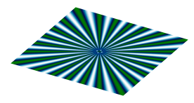
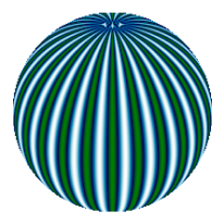
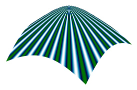
Figure 5. Illustrations of the laminate-like structure of the coefficient field on $\mathbb{R}^{2}$, $\mathbb{S}^{2}$ and $\mathbb{H}^{2}$.

We make the following observations:

1. By Theorem 4 we have $\mathbb{L}_{\varepsilon}\stackrel{{\scriptstyle H}}{{\to}}\mathbb{L}_{0}$ for a subsequence and some coefficient field $\mathbb{L}_{0}$. As we shall see below, the limit $\mathbb{L}_{0}$ can be expressed by a “homogenization formula” that uniquely determines $\mathbb{L}_{0}$ in terms of $\mathbb{L}_{\#}$. Hence, $\mathbb{L}_{0}$ is independent of the chosen subsequence and we conclude that $\mathbb{L}_{\varepsilon}\stackrel{{\scriptstyle H}}{{\to}}\mathbb{L}_{0}$ for all sequences $\varepsilon\downarrow 0$.

2. Consider the special case

   (28) $$\mathbb{L}_{\#}(r,\theta,y):=\begin{pmatrix}a_{\#}(y)&0\\ 0&b_{\#}(y)\end{pmatrix}$$

   with $a_{\#},b_{\#}:\mathbb{R}\hskip 0.5pt\to(\lambda,\Lambda)$ measurable and $1$-periodic. Above, we tacitly expressed $\mathbb{L}_{\#}$ w.r.t. polar coordinates, i.e. $(\mathbb{L}_{\#})_{ij}:=(\tfrac{\partial}{\partial x^{i}},\mathbb{L}_{\#}\tfrac{\partial}{\partial x^{j}})$ where $x=(x^{1},x^{2})=(r,\theta)$. In this case we may represent $\mathbb{L}_{0}$ with help of the arithmetic and harmonic mean of $a_{\#}$ and $b_{\#}$ to express the diffusivity orthogonal to the flow $\phi$ and aligned to the flow $\phi$, respectively:

   (29) $$\mathbb{L}_{0}=\begin{pmatrix}\int_{0}^{1}a_{\#}&0\\ 0&(\int_{0}^{1}b_{\#}^{-1})^{-1}\end{pmatrix}.$$

In order to prove these claims it suffices to identify $\mathbb{L}_{0}$ locally. Consider an open, bounded set $\omega\Subset M$. We may assume without loss of generality that $\overline{\omega}$ does not intersect the curve $\{(r,\theta)\,:\,\theta=0\}$. Denote the chart of polar coordinates by $\Psi$ and define $U\subset\mathbb{R}^{2}$ by $U:=\Psi(\omega)$. According to (16) we associate to $\mathbb{L}_{\varepsilon}$ a coefficient field $A_{\varepsilon}$ on $U$. It can be written in the form $A_{\varepsilon}(r,\theta)=A_{\#}(r,\theta,\tfrac{\theta}{\varepsilon})$ with

$$A_{\#}(r,\theta,y)=\begin{pmatrix}s(r)&0\\ 0&s^{-1}(r)\end{pmatrix}\mathbb{L}_{\#}(r,\theta,y),$$

where we identified $\mathbb{L}_{\#}(r,\theta,y)$ with the corresponding coefficient matrix in polar coordinates. Since $\mathbb{L}_{\varepsilon}\stackrel{{\scriptstyle H}}{{\to}}\mathbb{L}_{0}$ on $\omega$, we have $A_{\varepsilon}\stackrel{{\scriptstyle H}}{{\to}}A_{0}$ on $U$ by Lemma 12. On the other hand, since $A_{\varepsilon}$ is a coefficient field of the form $A_{\#}(r,\theta,\frac{\theta}{\varepsilon})$ with $A_{\#}$ being continuous in the first two components and periodic in the third component, the periodic homogenization formula (21) applies and we deduce that $A_{0}$ only depends on $\mathbb{L}_{\#}$ and the metric $g$ (but not on the extracted subsequence). Hence, $\mathbb{L}_{0}$ is uniquely determined by $\mathbb{L}_{\#}$ and the metric, and thus $H$-convergence holds for the entire sequence. This proves (a)

Next, we discuss the special case (28) for which we obtain

$$A_{\#}(r,\theta,y)=\begin{pmatrix}s(r)a_{\#}\left({\frac{\theta}{\varepsilon}}\right)&0\\ 0&s^{-1}(r)b_{\#}\left({\frac{\theta}{\varepsilon}}\right)\end{pmatrix}$$

and

$$A_{0}(r,\theta)=\begin{pmatrix}s(r)\int_{0}^{1}a_{\#}&0\\ 0&s^{-1}(r)(\int_{0}^{1}b_{\#}^{-1})^{-1}\end{pmatrix}.$$

The above identities can be seen by evaluating (21), which in the case of laminates can be done by hand. This proves (b).

Example 1: A graphical surface with star-shaped corrugations

In the spirit of Definition 1 we start with the reference manifold

$$M_{0}=\{(r,\theta);r\in(0,R),\theta\in[0,2\pi)\}$$

for some $R>0$. Note that $M_{0}$ does not include the origin. Now we define a family $M_{\varepsilon}=h_{\varepsilon}(M_{0})$ of $2$-dimensional submanifolds of $\mathbb{R}^{3}$ (with standard metric and measure induced from $\mathbb{R}^{3}$) using uniform bi-Lipschitz immersions $h_{\varepsilon}\colon M_{0}\to\mathbb{R}^{3}$,

$$h_{\varepsilon}(r,\theta)=\begin{pmatrix}r\sin\theta\\ r\cos\theta\\ \varepsilon f(r,\tfrac{\theta}{\varepsilon})\end{pmatrix},$$

where $f\colon(0,\infty)\times[0,\infty)\to\mathbb{R}$ is smooth and $2\pi$-periodic in the second argument. In Figure 1 in the Introduction we choose $f(r,y)=\sin^{2}(y)$ to present $M_{\varepsilon}$ for some values of $\varepsilon$.

We follow the path described in Lemma 20 and calculate first

$$dh_{\varepsilon}^{\sf T}dh_{\varepsilon}=\begin{pmatrix}1+\bigl{(}\varepsilon\partial_{1}f(r,\tfrac{\theta}{\varepsilon})\bigr{)}^{2}&\varepsilon\partial_{1}f(r,\tfrac{\theta}{\varepsilon})\partial_{2}f(r,\tfrac{\theta}{\varepsilon})\\ \varepsilon\partial_{1}f(r,\tfrac{\theta}{\varepsilon})\partial_{2}f(r,\tfrac{\theta}{\varepsilon})&r^{2}+\bigl{(}\partial_{2}f(r,\tfrac{\theta}{\varepsilon})\bigr{)}^{2}\end{pmatrix},$$

to get the density

$$\rho_{\varepsilon}=\sqrt{\det(dh_{\varepsilon}^{\sf T}dh_{\varepsilon})}=\sqrt{r^{2}+r^{2}\bigl{(}\varepsilon\partial_{1}f(r,\tfrac{\theta}{\varepsilon})\bigr{)}^{2}+\bigl{(}\partial_{2}f(r,\tfrac{\theta}{\varepsilon})\bigr{)}^{2}},$$

and the coefficient field

$$\mathbb{L}_{\varepsilon} =\rho_{\varepsilon}(dh_{\varepsilon}^{\sf T}dh_{\varepsilon})^{-1}$$

$$=1/\rho_{\varepsilon}\begin{pmatrix}r^{2}+\bigl{(}\partial_{2}f(r,\tfrac{\theta}{\varepsilon})\bigr{)}^{2}&-\varepsilon\partial_{1}f(r,\tfrac{\theta}{\varepsilon})\partial_{2}f(r,\tfrac{\theta}{\varepsilon})\\ -\varepsilon\partial_{1}f(r,\tfrac{\theta}{\varepsilon})\partial_{2}f(r,\tfrac{\theta}{\varepsilon})&1+\bigl{(}\varepsilon\partial_{1}f(r,\tfrac{\theta}{\varepsilon})\bigr{)}^{2}\end{pmatrix}.$$

It turns out that $\rho_{\varepsilon}\stackrel{{\scriptstyle*}}{{\rightharpoonup}}\rho_{0}$ weakly-$*$ in $L^{\infty}(M_{0})$ with

$$\rho_{0}(r)=\tfrac{1}{2\pi}\int_{0}^{2\pi}\sqrt{\bigl{(}\partial_{2}f(r,y)\bigr{)}^{2}+r^{2}}\,\mathrm{d}y,$$

and using (29) we see $\mathbb{L}_{\varepsilon}\overset{H}{\to}\mathbb{L}_{0}$ with

$$\mathbb{L}_{0} =\begin{pmatrix}\tfrac{1}{2\pi}\int_{0}^{2\pi}\sqrt{\bigl{(}\partial_{2}f(r,y)\bigr{)}^{2}+r^{2}}\,\mathrm{d}y&0\\ 0&\Bigl{(}\tfrac{1}{2\pi}\int_{0}^{2\pi}\sqrt{\bigl{(}\partial_{2}f(r,y)\bigr{)}^{2}+r^{2}}\,\mathrm{d}y\Bigr{)}^{-1}\end{pmatrix}$$

$$=\begin{pmatrix}\rho_{0}(r)&0\\ 0&\tfrac{1}{\rho_{0}(r)}\end{pmatrix}.$$

Thus the limiting metric on $M_{0}$ is given by

$$\hat{g}_{0}(\xi,\eta)=\rho_{0}\mathbb{L}_{0}^{-1}\xi\cdot\eta=\begin{pmatrix}1&0\\ 0&\rho_{0}^{2}\end{pmatrix}\xi\cdot\eta.$$

In this situation we finally can find a bi-Lipschitz immersion $h_{0}\colon M_{0}\to\mathbb{R}^{3}$ such that $dh_{0}^{\sf T}dh_{0}=\rho_{0}\mathbb{L}_{0}^{-1}$, namely

$$h_{0}(r,\theta)=\begin{pmatrix}\rho_{0}(r)\sin\theta\\ \rho_{0}(r)\cos\theta\\ \int_{0}^{r}\sqrt{1-\rho_{0}^{\prime}(t)^{2}}\,\mathrm{d}t\end{pmatrix}.$$

That means, by Remark 21, the (rotationally symmetric) submanifold $N_{0}:=h_{0}(M_{0})$ of $\mathbb{R}^{3}$ (with the standard measure and metric induced from $\mathbb{R}^{3}$), which for the case $f(r,y)=\sin^{2}(y)$ is pictured in Figure 1, is the spectral limit of $(M_{\varepsilon})$. Note that the excluded origin in the reference manifold coincides now with a circle of radius $\lim_{r\downarrow 0}\rho_{0}(r)$, which for $f(r,y)=\sin^{2}(y)$ is $\tfrac{\pi}{2}$.

Example 2: Sphere with radial perturbations oscillating with the longitude

Instead of a graph over $\mathbb{R}^{2}$ as in the example above we can treat a radially perturbed sphere in the same way. We take an analogous underlying reference manifold

$$M_{0}=\{(\varphi,\theta);\varphi\in(0,\pi),\theta\in[0,2\pi)\}$$

and define the family $M_{\varepsilon}:=h_{\varepsilon}(M_{0})$ of $2$-dimensional submanifolds of $\mathbb{R}^{3}$ via bi-Lipschitz immersions $h_{\varepsilon}\colon M_{0}\to M_{\varepsilon}$,

$$h_{\varepsilon}(\varphi,\theta)=\bigl{(}1+\varepsilon f(\varphi,\tfrac{\theta}{\varepsilon})\bigr{)}\begin{pmatrix}\sin\varphi\sin\theta\\ \sin\varphi\cos\theta\\ \cos\varphi\end{pmatrix},$$

where $f\colon(0,\pi)\times[0,\infty)\to\mathbb{R}$ is differentiable and $2\pi$-periodic in the second argument. In Figure 2 in the Introduction we choose $f(r,y)=\sin^{2}(y)$ to picture $M_{\varepsilon}$ for some values of $\varepsilon$. As in the previous example we obtain the following formulas for the limiting density

$$\rho_{0}(\varphi)=\tfrac{1}{2\pi}\int_{0}^{2\pi}\sqrt{(\partial_{2}f(\varphi,y))^{2}+\sin^{2}\varphi}\,\mathrm{d}y,$$

and the limiting metric

$$\hat{g}_{0}(\xi,\eta)=\tfrac{1}{\rho_{0}}\mathbb{L}_{0}=\begin{pmatrix}1&0\\ 0&\rho_{0}^{2}\end{pmatrix}\xi\cdot\eta.$$

Again we can find a bi-Lipschitz immersion $h_{0}\colon M_{0}\to\mathbb{R}^{3}$ such that $dh_{0}^{\sf T}dh_{0}=\rho_{0}\mathbb{L}_{0}^{-1}$, namely

$$h_{0}(\varphi,\theta)=\begin{pmatrix}\rho_{0}(\varphi)\sin\theta\\ \rho_{0}(\varphi)\cos\theta\\ \int_{0}^{\varphi}\sqrt{1-\rho_{0}^{\prime}(t)^{2}}\,\mathrm{d}t\end{pmatrix}.$$

Thus the (rotationally symmetric) submanifold $N_{0}:=h_{0}(M_{0})$ of $\mathbb{R}^{3}$, which for the case $f(r,y)=\sin^{2}(y)$ is pictured in Figure 2, is the spectral limit of the sequence $(M_{\varepsilon})$.

3.2. Concentric laminate-like coefficient fields on Voronoi tesselated manifolds

Let $(M,g,\mu)$ be a $n$-dimensional manifold and $Z\subset M$ a countable closed subset. For $z\in Z$ we denote by $M_{z}$ the associated Voronoi cell, that is

$$M_{z}:=\{x\in M;d(x,z)<d(x,Z\setminus\{z\})\},$$

where $d(\cdot,\cdot)$ is the geodesic distance on $M$. We assume the Voronoi tessellation to be fine enough to ensure that for $\mu$-a.e. point $x_{0}\in M$ there are $z\in Z$ and $\varrho>0$ such that

(30) $$\text{for all }x\in B_{\varrho}(x_{0})\subset M_{z}\text{ exists exactly one shortest path }\gamma_{x}\text{ from }x\text{ to }z.$$

We consider a sequence $(\mathbb{L}_{\varepsilon})$ in $\mathcal{M}(M,\lambda,\Lambda)$ of rapidly oscillating coefficient fields of the form $\mathbb{L}_{\varepsilon}(x)=\mathbb{L}(\tfrac{d(x,Z)}{\varepsilon})$, where $\mathbb{L}(r)$ is $1$-periodic in $r\in\mathbb{R}\hskip 0.5pt$, see Figure 6.

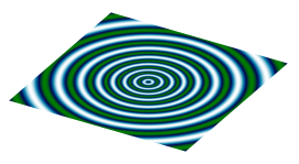
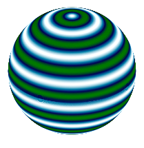
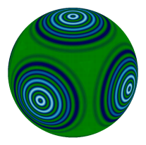
Figure 6. Illustration of coefficient fields with laminate-like structure.

By Theorem 4 $(\mathbb{L}_{\varepsilon})$ $H$-converges (up to a subsequence) to some $\mathbb{L}_{0}\in\mathcal{M}(M,\lambda,\Lambda)$. We are going to show that $\mathbb{L}_{0}$ coincides $\mu$-a.e. on $M$ with some constant coefficient field which is uniquely determined by $\mathbb{L}$. In particular the whole sequence $(\mathbb{L}_{\varepsilon})$ $H$-converges to $\mathbb{L}_{0}$.

In order to prove this, it suffices to identify $\mathbb{L}_{0}$ locally, i.e. for $\mu$-a.e. $x_{0}\in M$. As a first step we construct curvilinear coordinates such that in these coordinates the coefficients locally turn into a laminate up to a small perturbation that vanishes at $x_{0}$. In particular we claim that local coordinates $(B_{\varrho}(x_{0}),\Psi;x^{1},\dotsc,x^{n})$ exist such that

(31a) $$\Psi(x_{0})=0,$$

(31b) $$x^{1}=d(\cdot,z)-d(x_{0},z),$$

(31c) $$g(\tfrac{\partial}{\partial x^{1}},\tfrac{\partial}{\partial x^{j}})=0\text{ for $j=2,\dotsc,n$},$$

(31d) $$\lim\limits_{x\to x_{0}}\rho(x)g(\tfrac{\partial}{\partial x^{i}},\tfrac{\partial}{\partial x^{j}})(x)=\delta_{ij}.$$

Indeed, note that by (31b) geodesics through $z$ are mapped to straight lines parallel to the $x^{1}$-axis.

Therefore, we fix $x_{0}\in M$, $z\in Z$ and $\varrho>0$ satisfying (30). As in (31b) we set for $x\in B_{\varrho}(x_{0})$

$$x^{1}(x):=d(x,z)-d(x_{0},z).$$

Thanks to (30) $x^{1}$ is differentiable and the level set $U_{x_{0}}:=\{x\in B_{\rho}(x_{0});x^{1}(x)=0\}$ is a $n-1$-dimensional submanifold of $M_{z}$ including $x_{0}$ and for any point $x\in U_{x_{0}}$ the tangent space $T_{x}U_{x_{0}}$ is orthogonal to $d\gamma_{x}(0)$, which gives (31c). Assume $\varrho>0$ to be small enough such that we can choose local normal coordinates $x^{2},\dotsc,x^{n}$ of $U_{x_{0}}$ with $x^{j}(x_{0})=0$ ($j=2,\dotsc,n$). By the differentiability of geodesics we can extend these coordinate functions to curvilinear coordinates $x^{1},\dotsc,x^{n}$ on $B_{\varrho}(x_{0})$ (with a probably smaller $\varrho$) in the way that $x^{2},\dotsc,x^{n}$ are constant on $\gamma_{x}$ for every $x\in B_{\varrho}(x_{0})$. Then we have

(32) $$\lim\limits_{x\to x_{0}}g(\tfrac{\partial}{\partial x^{i}},\tfrac{\partial}{\partial x^{j}})(x)=\begin{cases}1,&i=j,\\ 0,&i\neq j,\end{cases}$$

which yields (31d).

Figure 7. Construction of the local coordinates

In these coordinates the associated coefficient field at $y\in U:=\Psi(B_{\varrho}(x_{0}))$ can be written as

$$A_{\varepsilon}(y)=A(y,\tfrac{y_{1}+d(x_{0},z)}{\varepsilon})$$

for some $A\colon U\times\mathbb{R}$ continuous in the first, and measurable and $1$-periodic in the second argument. This can be seen by considering (16): The coefficient field $A_{\varepsilon}$ on $U$ associated to $\mathbb{L}_{\varepsilon}$ takes the form

$$(A_{\varepsilon})_{ij}=\overline{\rho}\,\overline{g}(\mathbb{L}_{\varepsilon}\nabla_{g}x^{i},\nabla_{g}x^{j}),$$

where $\overline{\rho}:=\rho\circ\Psi^{-1}$ and $\overline{g}:=g\circ\Psi^{-1}$ denote the representation of the quantities in local coordinates. By the definitions of $\mathbb{L}_{\varepsilon}$ and $x^{1}$ we see that

$$g(\mathbb{L}_{\varepsilon}(x)\tfrac{\partial}{\partial x^{i}},\tfrac{\partial}{\partial x^{j}})=g(\mathbb{L}(\tfrac{d(x,Z)}{\varepsilon})\tfrac{\partial}{\partial x^{i}},\tfrac{\partial}{\partial x^{j}})=g(\mathbb{L}(\tfrac{x^{1}(x)+d(x_{0},Z)}{\varepsilon})\tfrac{\partial}{\partial x^{i}},\tfrac{\partial}{\partial x^{j}})$$

is only depending on $x^{1}(x)=y_{1}$, and $A_{\varepsilon}$ has the desired form with

(33) $$A_{ij}(y,r):=\overline{\rho}\,\overline{g}(\mathbb{L}(r)\nabla_{g}x^{i},\nabla_{g}x^{j})(y),$$

which is continuous in $y\in U$, and measurable and $1$-periodic in $r\in\mathbb{R}$.

For $\varepsilon\to 0$ the homogenized matrix $A_{\text{hom}}$ associated with $A_{\varepsilon}$ is given by the homogenization formula (21) for $A$ defined in (33). Therefore $A_{\text{hom}}$ continuously depends on $y\in U$. Moreover the matrix $A_{\text{hom}}(0)$ is independent on the initial choice of $x_{0}$ and is given by the following weak-$*$ limits in $L^{\infty}(U)$:

$$\frac{1}{A_{11}(0,\tfrac{\cdot}{\varepsilon})}\rightharpoonup\frac{1}{(A_{\text{hom}})_{11}(0)},$$

$$\frac{A_{i1}(0,\tfrac{\cdot}{\varepsilon})}{A_{11}(0,\tfrac{\cdot}{\varepsilon})}\rightharpoonup\frac{(A_{\text{hom}})_{i1}(0)}{(A_{\text{hom}})_{11}(0)},\quad i=2,\dotsc,n,$$

$$\frac{A_{1j}(0,\tfrac{\cdot}{\varepsilon})}{A_{11}(0,\tfrac{\cdot}{\varepsilon})}\rightharpoonup\frac{(A_{\text{hom}})_{1j}(0)}{(A_{\text{hom}})_{11}(0)},\quad j=2,\dotsc,n,$$

$$A_{ij}(0,\tfrac{\cdot}{\varepsilon})-\frac{A_{i1}(0,\tfrac{\cdot}{\varepsilon})A_{1j}(0,\tfrac{\cdot}{\varepsilon})}{A_{11}(0,\tfrac{\cdot}{\varepsilon})}\rightharpoonup(A_{\text{hom}})_{ij}(0)-\frac{(A_{\text{hom}})_{i1}(0)(A_{\text{hom}})_{1j}(0)}{(A_{\text{hom}})_{11}(0)},\quad i,j=2,\dotsc,n.$$

By Lemma 14, we have

$$(A_{\text{hom}})_{ij}=\overline{\rho}\,\overline{g}(\mathbb{L}_{0}\nabla_{g}x^{i},\nabla_{g}x^{j}).\qquad\text{a.e.~{}in }U,$$

We conclude that $\mathbb{L}_{0}$ is continuous ($\mu$-a.e.) on $B_{\varrho}(x_{0})$ and thus (using (32)) $g(\mathbb{L}_{0}(x_{0})\tfrac{\partial}{\partial x^{i}},\tfrac{\partial}{\partial x^{j}})(x_{0})=(A_{\text{hom}})_{ij}(0)$ for $\mu$-a.e. $x_{0}\in M$.

As in the previous example we could consider the special case of a diagonal matrix

$$\mathbb{L}(r)\tfrac{\partial}{\partial x^{i}}=a_{i}(r)\tfrac{\partial}{\partial x^{i}}\qquad\text{for $i=1,\dotsc,n$}.$$

Then $\mathbb{L}_{0}(x_{0})$ is a diagonal matrix, too, and we have

(34) $$g(\mathbb{L}_{0}(x_{0})\tfrac{\partial}{\partial x^{1}},\tfrac{\partial}{\partial x^{1}})(x_{0})=\Big{(}\int_{0}^{1}a_{1}^{-1}\Big{)}^{-1}\qquad\text{and}$$

$$g(\mathbb{L}_{0}(x_{0})\tfrac{\partial}{\partial x^{i}},\tfrac{\partial}{\partial x^{i}})(x_{0})=\int_{0}^{1}a_{i}\qquad\text{for $i=2,\dotsc,n$}.$$

Example 3: A radially symmetric corrugated graphical surface

We consider the reference manifold

$$M_{0}=\{(r,\theta);r\in(0,R),\theta\in[0,2\pi)\}$$

for some $R>0$, and define a family $M_{\varepsilon}=h_{\varepsilon}(M_{0})$ of $2$-dimensional submanifolds of $\mathbb{R}^{3}$ using uniform bi-Lipschitz immersions $h_{\varepsilon}\colon M_{0}\to\mathbb{R}^{3}$,

(35) $$h_{\varepsilon}(r,\theta)=\begin{pmatrix}r\sin\theta\\ r\cos\theta\\ \varepsilon f(r,\tfrac{r}{\varepsilon})\end{pmatrix},$$

where $f(0,\infty)\times[0,\infty)\to\mathbb{R}$ is differentiable and $T$-periodic in the second argument. In Figure 8 we took $f(r,y)=\sin^{2}(y)$ to illustrate $M_{\varepsilon}$ for some values of $\varepsilon$.

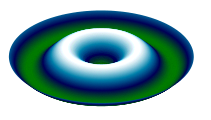
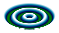
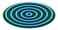
$\xrightarrow{\varepsilon\downarrow 0}$

$\varepsilon=\tfrac{1}{2}$

$\varepsilon=\tfrac{1}{4}$

$\varepsilon=\tfrac{1}{8}$

Figure 8. A family of rotationally symmetric corrugated graphical surfaces. The three pictures on the left show $M_{\varepsilon}$ defined via (35) with $f=\sin^{2}$ and decreasing values of $\varepsilon$. The picture on the right shows the limiting surface $N_{0}$ defined via (36). As $\varepsilon\to 0$ the spectrum of the Laplace-Beltrami operator on $M_{\varepsilon}$ converges to the spectrum of the Laplace-Beltrami operator on $N_{0}$.

Following Lemma 20 we compute the density

$$\rho_{\varepsilon}=\sqrt{\det(dh_{\varepsilon}^{\sf T}dh_{\varepsilon})}=\sqrt{r^{2}+r^{2}\bigl{(}\varepsilon\partial_{1}f(r,\tfrac{r}{\varepsilon})+\partial_{2}f(r,\tfrac{r}{\varepsilon})\bigr{)}^{2}}.$$

and the coefficient field

$$\mathbb{L}_{\varepsilon} =\rho_{\varepsilon}(dh_{\varepsilon}^{\sf T}dh_{\varepsilon})^{-1}$$

$$=1/\rho_{\varepsilon}\begin{pmatrix}r^{2}&0\\ 0&1+\bigl{(}\varepsilon\partial_{1}f(r,\tfrac{r}{\varepsilon})+\partial_{2}f(r,\tfrac{r}{\varepsilon})\bigr{)}^{2}\end{pmatrix}.$$

We find $\rho_{\varepsilon}\stackrel{{\scriptstyle*}}{{\rightharpoonup}}\rho_{0}$ weakly-$*$ in $L^{\infty}(M_{0})$ with

$$\rho_{0}(r)=\tfrac{r}{T}\int_{0}^{T}\sqrt{\bigl{(}\partial_{2}f(r,y)\bigr{)}^{2}+1}\,\mathrm{d}y,$$

and using (34) we see $\mathbb{L}_{\varepsilon}\overset{H}{\to}\mathbb{L}_{0}$ with

$$\mathbb{L}_{0} =\begin{pmatrix}\Bigl{(}\tfrac{1}{rT}\int_{0}^{T}\sqrt{\bigl{(}\partial_{2}f(r,y)\bigr{)}^{2}+1}\,\mathrm{d}y\Bigr{)}^{-1}&0\\ 0&\tfrac{1}{rT}\int_{0}^{T}\sqrt{\bigl{(}\partial_{2}f(r,y)\bigr{)}^{2}+1}\,\mathrm{d}y\end{pmatrix}$$

$$=\begin{pmatrix}\tfrac{r^{2}}{\rho_{0}(r)}&0\\ 0&\tfrac{\rho_{0}(r)}{r^{2}}\end{pmatrix}.$$

and get the limiting metric on $M_{0}$:

$$\hat{g}_{0}(\xi,\eta)=\rho_{0}\mathbb{L}_{0}^{-1}\xi\cdot\eta=\begin{pmatrix}\tfrac{\rho_{0}(r)^{2}}{r^{2}}&0\\ 0&r^{2}\end{pmatrix}\xi\cdot\eta.$$

We finally find a bi-Lipschitz immersion $h_{0}\colon M_{0}\to\mathbb{R}^{3}$ such that $dh_{0}^{\sf T}dh_{0}=\rho_{0}\mathbb{L}_{0}^{-1}$, namely

(36) $$h_{0}(r,\theta)=\begin{pmatrix}r\sin\theta\\ r\cos\theta\\ \int_{0}^{r}\sqrt{\tfrac{\rho_{0}(t)^{2}}{t^{2}}-1}\,\mathrm{d}t\end{pmatrix}.$$

By Remark 21, the submanifold $N_{0}:=h_{0}(M_{0})$ of $\mathbb{R}^{3}$, which for the case $f(r,y)=\sin^{2}(y)$ is shown in Figure 8, is the spectral limit of $(M_{\varepsilon})$.

Example 4: Sphere with radial perturbations oscillating with the latitude.

In the same way as in the previous example we can handle the case of a radially perturbed sphere. Again we start with the reference manifold

$$M_{0}=\{(\varphi,\theta);\varphi\in(0,\pi),\theta\in[0,2\pi)\}$$

and define the family $M_{\varepsilon}:=h_{\varepsilon}(M_{0})$ of $2$-dimensional submanifolds of $\mathbb{R}^{3}$ via bi-Lipschitz immersions $h_{\varepsilon}\colon\overline{M}\to M_{\varepsilon}$,

$$h_{\varepsilon}(\varphi,\theta)=\bigl{(}1+\varepsilon f(\varphi,\tfrac{\varphi}{\varepsilon})\bigr{)}\begin{pmatrix}\sin\varphi\sin\theta\\ \sin\varphi\cos\theta\\ \cos\varphi\end{pmatrix},$$

where $f\colon(0,\pi)\times[0,\infty)\to\mathbb{R}$ is differentiable and $2\pi$-periodic in the second argument. In Figure 3 in the Introduction we choose $f(r,y)=\sin^{2}(y)$ to picture $M_{\varepsilon}$ for some values of $\varepsilon$.

Doing the same calculations as in the example above we end up with the density

$$\rho_{0}(\varphi)=\tfrac{\sin\varphi}{\pi}\int_{0}^{\pi}\sqrt{(\partial_{2}f(\varphi,y))^{2}+1}\,\mathrm{d}y,$$

and the metric

$$\tfrac{1}{\rho_{0}}\mathbb{L}_{0}=\begin{pmatrix}\tfrac{\sin^{2}\varphi}{\rho_{0}(\varphi)^{2}}&0\\ 0&\tfrac{1}{\sin^{2}\varphi}\end{pmatrix}.$$

and again we find a bi-Lipschitz immersion $h_{0}\colon M_{0}\to\mathbb{R}^{3}$ such that $dh_{0}^{\sf T}dh_{0}=\rho_{0}\mathbb{L}_{0}^{-1}$, namely

$$h_{0}(\varphi,\theta)=\begin{pmatrix}\sin\varphi\sin\theta\\ \sin\varphi\cos\theta\\ \int_{0}^{\varphi}\sqrt{\tfrac{\rho_{0}(t)^{2}}{\sin^{2}t}-\cos^{2}t}\,\mathrm{d}t\end{pmatrix}.$$

Thus the submanifold $N_{0}:=h_{0}(M_{0})$ of $\mathbb{R}^{3}$, which for the case $f(r,y)=\sin^{2}(y)$ is pictured in Figure 3, is the spectral limit of the sequence $(M_{\varepsilon})$.

Example 5: A locally corrugated graphical surface

We finally want to discuss an example with oscillations in several Voronoi cells which can be treated locally.

Let $Y\subset\mathbb{R}^{2}$ be relatively-compact and open. Consider a set $Z\in Y$ of isolated points. For every point $z\in Z$ we use a smooth function $\psi_{z}\colon[0,\infty)\to[0,1]$ to define a rotationally symmetric cut-off function $\psi_{z}(|\cdot-z|)$ such that

$$\begin{cases}\text{$\psi_{z}(0)=1$,}&\\ \text{$\mathrm{supp}\psi_{z}(|\cdot-z|)\cap\mathrm{supp}\psi_{z^{\prime}}(|\cdot-z^{\prime}|)=\emptyset$ for all $z^{\prime}\in Z\setminus\{z\}$.}\end{cases}$$

Now we consider a smooth $T$-periodic function $f\colon[0,\infty)\to\mathbb{R}$ and define $M_{\varepsilon}$ as the graph of the function $h_{\varepsilon}\colon M_{0}:=Y\setminus Z\to\mathbb{R}$,

$$h_{\varepsilon}(x):=\sum_{z\in Z}\varepsilon f\big{(}\tfrac{|x-z|}{\varepsilon}\big{)}\psi_{z}(|x-z|)\in\mathbb{R}^{3},$$

which we regard as a two-dimensional submanifold of $\mathbb{R}\hskip 0.5pt^{3}$. In Figure 4 in the Introduction we took $f(y)=\sin^{2}(y)$ to show $M_{\varepsilon}$ for some values of $\varepsilon$.

Doing the same calculations as in the previous examples locally in each Voronoi cell we get a function $h_{0}\colon M_{0}\to\mathbb{R}$,

$$h_{0}(x):=x\mapsto\sum_{z\in Z}\int_{0}^{|x-z|}\sqrt{\tfrac{\rho_{0,z}(t)^{2}}{t^{2}}-1}\,\mathrm{d}t\in\mathbb{R}^{3},$$

where $\rho_{0,z}(r)=\tfrac{r}{T}\int_{0}^{T}\sqrt{f^{\prime}(y)^{2}\psi_{z}(r)^{2}+1}\,\mathrm{d}y$, such that the graph of $h_{0}$, which is shown in Figure 4 for $f(y)=\sin^{2}(y)$, is the spectral limit of $(M_{\varepsilon})$.

4. Proofs

4.1. Proof of Proposition 5, Lemma 6 and Lemma 7

The argument consists of two parts. In the first part we identify the limiting tensor field $\mathbb{L}_{0}$. For this purpose, we consider the operators

(37) $$\mathcal{L}_{\varepsilon}^{*}\colon H^{1}_{0}(B)\to H^{-1}(B),\qquad\mathcal{L}_{\varepsilon}^{*}u:=-{\mathop{\operatorname{div}}}(\mathbb{L}_{\varepsilon}^{*}\nabla),$$

where $\mathbb{L}_{\varepsilon}^{*}$ denotes the adjoint of $\mathbb{L}_{\varepsilon}$ and is defined by the identity $(\mathbb{L}_{\varepsilon}^{*}\xi,\eta)=(\xi,\mathbb{L}_{\varepsilon}\eta)$ for all vector fields $\xi,\eta$. Since the operator is uniformly elliptic (with constants independent of $\varepsilon$) we can deduce the existence of a linear isomorphism $\mathcal{L}_{0}^{*}$, whose inverse is the limit of $(\mathcal{L}_{\varepsilon}^{*})^{-1}$ in the weak operator topology. Indeed, this follows from the following standard compactness result:

Lemma 22.

Let $V$ be a reflexive separable Banach space and $(T_{\varepsilon})$ be a sequence of linear operators $T_{\varepsilon}\colon V\to V^{\prime}$ that is uniformly bounded and coercive, i.e. there exists $C>0$ (independent of $\varepsilon$) such that the operator norm of $T_{\varepsilon}$ is bounded by $C$ and

(38) $$\langle T_{\varepsilon}v,v\rangle_{V^{\prime},V}\geq\tfrac{1}{C}\|v\|_{V}^{2}\qquad\text{for all }v\in V.$$

Then there exists a linear bounded operator $T_{0}\colon V\to V^{\prime}$ satisfying $\eqref{eq6.0708}$ and for a subsequence (not relabeled) we have $T_{\varepsilon}^{-1}\rightharpoonup T_{0}^{-1}$ in the weak operator topology, that is for all $f\in V^{\prime}$ we have

$$T_{\varepsilon}^{-1}f\rightharpoonup T_{0}^{-1}f\qquad\text{weakly in }V.$$

(For a proof, e.g., see [25, Proposition 4]). We then show that $\mathcal{L}_{0}^{*}$ can in fact be written in divergence form: $\mathcal{L}_{0}^{*}=-{\mathop{\operatorname{div}}}(\mathbb{L}_{0}^{*}\nabla)$ with an appropriate $(1,1)$-tensor field $\mathbb{L}_{0}^{*}$. In order to define $\mathbb{L}_{0}^{*}$ with help of $\mathcal{L}_{0}^{*}$, we introduce auxiliary functions whose gradients span the tangent space. More precisely, we recall the following fact:

Remark 23.

Let $B\Subset M$ denote an open ball with radius smaller than the injectivity radius at its center. Then there exist $v_{1},\dotsc,v_{n}\in C^{\infty}_{c}(B)$ such that $T(\frac{1}{2}B)$ is spanned by the vector fields $\nabla v_{1},\dotsc,\nabla v_{n}$, i.e.

(39) $$\forall y\in\tfrac{1}{2}B\,:\qquad T_{y}(\tfrac{1}{2}B)=\operatorname{span}\{\nabla v_{1}(y),\dotsc,\nabla v_{n}(y)\}.$$

Following ideas of Tartar and Murat, we associate with $v_{1},\ldots,v_{n}$ oscillating test-functions $v_{1,\varepsilon},\ldots,v_{n,\varepsilon}$ that allow to pass to the limit in products of weakly convergent sequences of the form $(\mathbb{L}_{\varepsilon}\nabla u_{\varepsilon},\nabla v_{i,\varepsilon})$. The argument invokes the following variant of the Div-Curl Lemma for manifolds:

Lemma 24 (Div-Curl Lemma).

Let $\Omega\subset M$ be open and let $(\xi_{\varepsilon})\subset L^{2}(T\Omega)$, $(v_{\varepsilon})\subset H^{1}(\Omega)$ denote sequences such that

$$\begin{cases}\xi_{\varepsilon}\rightharpoonup\xi&\text{weakly in }L^{2}(T\Omega),\\ {\mathop{\operatorname{div}}}\xi_{\varepsilon}\to{\mathop{\operatorname{div}}}\xi&\text{in }H^{-1}(\Omega),\\ \end{cases}\qquad\text{and}\qquad v_{\varepsilon}\rightharpoonup v\quad\text{weakly in }H^{1}(\Omega).$$

Then

$$\int_{\Omega}(\xi_{\varepsilon},\nabla v_{\varepsilon})\varphi\,\mathrm{d}\mu\to\int_{\Omega}(\xi,\nabla v)\varphi\,\mathrm{d}\mu\qquad\text{for all }\varphi\in C^{\infty}_{c}(\Omega).$$

Moreover, if $v_{\varepsilon},v\in H^{1}_{0}(\Omega)$, then

$$\int_{\Omega}(\xi_{\varepsilon},\nabla v_{\varepsilon})\,\mathrm{d}\mu\to\int_{\Omega}(\xi,\nabla v)\,\mathrm{d}\mu.$$

We present the short proof for the reader’s convenience:

Proof of Lemma 24.

In the case $v_{\varepsilon}\in H^{1}_{0}(\Omega)$ the statement follows by an integration by parts. In the general case, for $\varphi\in C_{c}^{\infty}(\Omega)$ we have

(40) $$\int_{\Omega}(\xi_{\varepsilon},\nabla v_{\varepsilon})\varphi=\int_{\Omega}(\xi_{\varepsilon},\nabla(v_{\varepsilon}\varphi))-\int_{\Omega}(\xi_{\varepsilon},v_{\varepsilon}\nabla\varphi)=-\langle{\mathop{\operatorname{div}}}\xi_{\varepsilon},v_{\varepsilon}\varphi\rangle-\int_{\Omega}(\xi_{\varepsilon},v_{\varepsilon}\nabla\varphi).$$

Regarding the first term of the right-hand side of (40),

$$-\langle{\mathop{\operatorname{div}}}\xi_{\varepsilon},v_{\varepsilon}\varphi\rangle\to-\langle{\mathop{\operatorname{div}}}\xi,v\varphi\rangle=\int_{\Omega}(\xi,v\nabla\varphi)+\int_{\Omega}(\xi,\varphi\nabla v).$$

For the second term of the right-hand side of (40), since $v_{\varepsilon}\rightharpoonup v$ in $H^{1}(\Omega)$, for any relatively compact open set $\Omega^{\prime}\subset M$, there exists a subsequence of $(v_{\varepsilon})$ converging to $v$ in $L^{2}(\Omega^{\prime})$ by Rellich’s theorem; in particular, $v_{\varepsilon}\nabla\varphi\to v\nabla\varphi$ in $L^{2}(TM)$ and thus $\int_{\Omega}(\xi_{\varepsilon},v_{\varepsilon}\nabla\varphi)\to\int_{\Omega}(\xi,v\nabla\varphi)$. Hence, the right-hand side of (40) converges to $\int_{\Omega}(\xi,\nabla v)\varphi$. ∎

In a second step, we then show that $\mathbb{L}_{0}$ (the adjoint of $\mathbb{L}_{0}^{*}$) is an $H$-limit of $(\mathbb{L}_{\varepsilon})$. To that end we need to consider for (arbitrary but fixed) subdomains $\omega\Subset\Omega$ the localized operators

(41) $$\mathcal{L}_{\varepsilon}\colon H^{1}_{0}(\omega)\to H^{-1}(\omega),\qquad\mathcal{L}_{\varepsilon}u:=-{\mathop{\operatorname{div}}}(\mathbb{L}_{\varepsilon}\nabla u),$$

and show that $\mathcal{L}_{\varepsilon}^{-1}\to\mathcal{L}_{0}^{-1}$ in the weak operator topology.

Proof of Proposition 5.

In the proof we pass to various subsequences and it turns out to be necessary to keep track of them. For a lean notation we denote by $E\subset(0,\infty)$ the set of $\varepsilon$’s of the given sequence $(\mathbb{L}_{\varepsilon})=(\mathbb{L}_{\varepsilon})_{\varepsilon\in E}$. We represent subsequences by means of subsets $E^{\prime},E^{\prime\prime},\dotsc\subset E$ that have a cluster point at $0$. We follow the convention to write

$$c_{\varepsilon}\to c_{0}\qquad(\varepsilon\in E^{\prime}),$$

if and only if for any sequence $(\varepsilon_{j})_{j\in\mathbb{N}}\subset E^{\prime}$ with $\varepsilon_{j}\to 0$ we have $c_{\varepsilon_{j}}\to c_{0}$.

Step 1. Choice of the subsequence and definition of $\mathbb{L}_{0}$.

Let $\mathcal{L}_{\varepsilon}^{*}$ be defined by (37) and fix $v_{1},\dotsc,v_{n}\in C^{\infty}_{c}(B)$ according to Remark 23. We claim that there exits a measurable $(1,1)$-tensor field $\mathbb{L}_{0}\colon\tfrac{1}{2}B\to\operatorname{Lin}(T(\tfrac{1}{2}B))$, a subsequence $E^{\prime}\subset E$, and functions $(v_{1,\varepsilon}),\dotsc,(v_{k,\varepsilon})\subset H^{1}_{0}(B)$ (the so called oscillating test functions) such that for $k=1,\dotsc,n$ and $\varepsilon\in E^{\prime}$ we have

(42) $$\begin{cases}v_{k,\varepsilon}\rightharpoonup v_{k}&\quad\mbox{weakly in }H^{1}_{0}(B),\\ v_{k,\varepsilon}\to v_{k}&\quad\mbox{in }L^{2}(B),\\ (\mathcal{L}_{\varepsilon}^{*}v_{k,\varepsilon})&\quad\mbox{strongly converges in }H^{-1}(B),\\ \mathbb{L}^{*}_{\varepsilon}\nabla v_{k,\varepsilon}\rightharpoonup\mathbb{L}^{*}_{0}\nabla v_{k}&\quad\mbox{weakly in }L^{2}(T(\tfrac{1}{2}B)).\end{cases}$$

For the argument note that by uniform ellipticity of $\mathbb{L}_{\varepsilon}^{*}$ and the boundedness of $B$, there exists $C=C(B,\lambda)>0$ such that

$$\langle\mathcal{L}_{\varepsilon}^{*}u,u\rangle=\int_{B}(\mathbb{L}_{\varepsilon}^{*}\nabla u,\nabla u)\geq C\|u\|^{2}_{H^{1}(B)},$$

and thus by Lemma 22 there is $\mathcal{L}_{0}^{*}\colon H^{1}_{0}(B)\to H^{-1}(B)$ and a subsequence $E^{\prime\prime}\subset E$ such that for all $f\in H^{-1}(B)$ and $\varepsilon\in E^{\prime\prime}$

$$(\mathcal{L}_{\varepsilon}^{*})^{-1}f\rightharpoonup(\mathcal{L}_{0}^{*})^{-1}f\qquad\mbox{weakly in }H^{1}_{0}(B).$$

For $k=1,\dotsc,n$ define

$$v_{k,\varepsilon}:=(\mathcal{L}_{\varepsilon}^{*})^{-1}\mathcal{L}_{0}^{*}v_{k},$$

which by uniform ellipticity of $\mathbb{L}_{\varepsilon}^{*}$ and Poincaré’s inequality in $H^{1}_{0}(B)$ are bounded uniformly in $\varepsilon$. Hence there exits vector fields $\ell_{1},\dotsc,\ell_{n}\in L^{2}(TB)$ and another subsequence $E^{\prime}\subset E^{\prime\prime}$ such that we have for $\varepsilon\in E^{\prime}$

$$\begin{cases}v_{k,\varepsilon}\rightharpoonup v_{k}&\quad\mbox{weakly in }H^{1}_{0}(B),\\ v_{k,\varepsilon}\to v_{k}&\quad\mbox{in }L^{2}(B),\\ \mathbb{L}_{\varepsilon}^{*}\nabla v_{k,\varepsilon}\rightharpoonup\ell_{k}&\quad\mbox{weakly in }L^{2}(TB).\end{cases}$$

Next, we define the tensor field $\mathbb{L}_{0}^{*}$ by the identity

$$\forall k\in\{1,\ldots,n\}\,:\qquad\mathbb{L}_{0}^{*}\nabla v_{k}=\ell_{k}\qquad\mu\text{-a.e.~{}in }\tfrac{1}{2}B.$$

Indeed, since $\nabla v_{1},\dotsc,\nabla v_{n}$ span $T(\tfrac{1}{2}B)$ the above identity defines $\mathbb{L}_{0}^{*}$ uniquely and the last identity in (42) is satisfied by construction. It remains to check the strong convergence of $(\mathcal{L}^{*}_{\varepsilon}v_{k,\varepsilon})$. In fact the stronger statement $\mathcal{L}^{*}_{\varepsilon}v_{k,\varepsilon}=\mathcal{L}_{0}^{*}v_{k}$ is valid, which is a direct consequence of the definition of $v_{k,\varepsilon}$.

Step 2. $H$-convergence of $\mathbb{L}_{\varepsilon}$ to $\mathbb{L}_{0}$ in $\frac{1}{2}B$.

Let the subsequence $E^{\prime}$, the tensor field $\mathbb{L}_{0}$, and $(v_{k,\varepsilon})$ be defined as in Step 1. We claim that $(\mathbb{L}_{\varepsilon})$ $H$-converges to $\mathbb{L}_{0}$ in $\tfrac{1}{2}B$ for $\varepsilon\in E^{\prime}$. To that end let $\omega\Subset\tfrac{1}{2}B$ and let $\mathcal{L}_{\varepsilon}$ be defined by (41). Arguing as in the previous step, we can find another subsequence $E^{\prime\prime}\subset E^{\prime}$ and a bounded linear, coercive operator $\mathcal{L}_{0}\colon H^{1}_{0}(\omega)\to H^{-1}(\omega)$ such that

(43) $$\mathcal{L}_{\varepsilon}^{-1}\rightharpoonup\mathcal{L}_{0}^{-1}\qquad\text{in the weak operator topology for }\varepsilon\in E^{\prime\prime}.$$

We only need to show that

(44) $$\mathcal{L}_{0}u_{0}=-{\mathop{\operatorname{div}}}(\mathbb{L}_{0}\nabla u_{0}),$$

for arbitrary $u_{0}\in H^{1}_{0}(\omega)$. For the argument set $u_{\varepsilon}:=\mathcal{L}_{\varepsilon}^{-1}\mathcal{L}_{0}u_{0}$ so that by (43),

(45) $$u_{\varepsilon}\rightharpoonup u_{0}\qquad\text{weakly in }H^{1}_{0}(\omega)\text{ and strongly in $L^{2}(\omega)$}\text{ for }\varepsilon\in E^{\prime\prime}.$$

Consider $J_{\varepsilon}:=\mathbb{L}_{\varepsilon}\nabla u_{\varepsilon}$. By uniform ellipticity of $\mathbb{L}_{\varepsilon}$ the sequences $(J_{\varepsilon})$ is bounded in $L^{2}(T\omega)$. Hence, there exits $J_{0}\in L^{2}(T\omega)$ and another subsequence $E^{\prime\prime\prime}\subset E^{\prime\prime}$ such that

(46) $$J_{\varepsilon}=\mathbb{L}_{\varepsilon}\nabla u_{\varepsilon}\rightharpoonup J_{0}\qquad\text{weakly in }L^{2}(T\omega)\text{ for }\varepsilon\in E^{\prime\prime\prime}.$$

Combined with the identity $-{\mathop{\operatorname{div}}}J_{\varepsilon}=\mathcal{L}_{0}u_{0}$ (which follows from the definition of $u_{\varepsilon}$) we find that

(47) $$-{\mathop{\operatorname{div}}}J_{0}=\mathcal{L}_{0}u_{0}.$$

Hence, for any test function $\varphi\in C^{\infty}_{c}(\omega)$, the convergence properties of $(v_{k,\varepsilon})$ yield

$$\int_{\omega}(J_{\varepsilon},\varphi\nabla v_{k,\varepsilon}) =\int_{\omega}(J_{\varepsilon},\nabla(\varphi v_{k,\varepsilon}))-\int_{\omega}(J_{\varepsilon},v_{k,\varepsilon}\nabla\varphi)$$

$$=\langle\mathcal{L}_{0}u_{0},\varphi v_{k,\varepsilon}\rangle-\int_{\omega}(J_{\varepsilon},v_{k,\varepsilon}\nabla\varphi)$$

$$\to\langle\mathcal{L}_{0}u_{0},\varphi v_{k}\rangle-\int_{\omega}(J_{0},v_{k}\nabla\varphi)$$

$$=\int_{\omega}(J_{0},\varphi\nabla v_{k}).$$

On the other hand, since $\mathbb{L}^{*}_{\varepsilon}\nabla v_{k,\varepsilon}\rightharpoonup\mathbb{L}^{*}_{0}\nabla v_{k}$ weakly in $L^{2}(T\tfrac{1}{2}B)$ and $(-{\mathop{\operatorname{div}}}(\mathbb{L}^{*}_{\varepsilon}\nabla v_{k,\varepsilon}))$ strongly converges in $H^{-1}(\frac{1}{2}B)$ by (42), the Div-Curl Lemma (Lemma 24) yields

$$\int_{\omega}(J_{\varepsilon},\varphi\nabla v_{k,\varepsilon})=\int_{\omega}(\varphi\nabla u_{\varepsilon},\mathbb{L}_{\varepsilon}^{*}\nabla v_{k,\varepsilon})\to\int_{\omega}(\varphi\nabla u_{0},\mathbb{L}^{*}_{0}\nabla v_{k})=\int_{\omega}(\mathbb{L}_{0}\nabla u_{0},\varphi\nabla v_{k}).$$

Hence, by combining the previous two identities we conclude that

$$\int_{\omega}(\mathbb{L}_{0}\nabla u_{0},\varphi\nabla v_{k})=\int_{\omega}(J_{0},\varphi\nabla v_{k}).$$

Since $\varphi\in C^{\infty}_{c}(\omega)$ is arbitrary and since $\nabla v_{1},\dotsc,\nabla v_{n}$ spans $T\omega$, we get $J_{0}=\mathbb{L}_{0}\nabla u_{0}$ $\mu$-a.e. in $\omega$. Thus (44) follows from (47). Moreover, since $J_{0}$ and $\mathcal{L}_{0}$ are uniquely determined by $\mathbb{L}_{0}$, the convergence in (43), (45), and (46) holds for the entire sequence $E^{\prime}$ (which in particular is independent of $\omega$).

Next we argue that $\mathbb{L}_{0}\in\mathcal{M}(\omega,\lambda,\Lambda)$. Indeed, from (45) and (46) and the Div-Curl Lemma (Lemma 24) we learn that for any non-negative $\varphi\in C^{\infty}_{c}(\omega)$ we have

$$\int_{\omega}(\mathbb{L}_{\varepsilon}\nabla u_{\varepsilon},\nabla u_{\varepsilon})\varphi\to\int_{\omega}(\mathbb{L}_{0}\nabla u_{0},\nabla u_{0})\varphi.$$

By uniform ellipticity of $\mathbb{L}_{\varepsilon}$ in form of (10), we have $\int_{\omega}(\mathbb{L}_{\varepsilon}\nabla u_{\varepsilon},\nabla u_{\varepsilon})\rho\geq\lambda\int_{\omega}|\nabla u_{\varepsilon}|^{2}\rho$, and thus

$$\int_{\omega}(\mathbb{L}_{0}\nabla u_{0},\nabla u_{0})\varphi\geq\lambda\int_{\omega}|\nabla u_{0}|^{2}\varphi.$$

Since this is true for all $u_{0}$ and $\varphi$, we conclude that $\mathbb{L}_{0}$ satisfies the lower ellipticity condition, cf. (10) $\mu$-a.e. in $\omega$. On the other hand (11) implies

$$\int_{\omega}(\mathbb{L}_{\varepsilon}\nabla u_{\varepsilon},\nabla u_{\varepsilon})\varphi=\int_{\omega}(\mathbb{L}_{\varepsilon}\nabla u_{\varepsilon},\mathbb{L}_{\varepsilon}^{-1}\mathbb{L}_{\varepsilon}\nabla u_{\varepsilon})\varphi\geq\Lambda\int_{\omega}|\mathbb{L}_{\varepsilon}\nabla u_{0}|^{2}\varphi,$$

and thus by the same reasoning as before, we get for $\mu$-a.e. $x\in\omega$ and all $\xi\in T_{x}\omega$

$$\Lambda|\mathbb{L}_{0}(x)\xi|^{2}\leq(\mathbb{L}_{0}(x)\xi,\xi).$$

Substituting $\xi=\mathbb{L}_{0}^{-1}(x)\xi^{\prime}$ yields the boundedness condition, cf. (11).

Since the above arguments hold for arbitrary $\omega\Subset\tfrac{1}{2}B$ we deduce that $\mathbb{L}_{0}\in\mathcal{M}(\frac{1}{2}B,\lambda,\Lambda)$ and that $(\mathbb{L}_{\varepsilon})$ $H$-converges to $\mathbb{L}_{0}$ in $\frac{1}{2}B$ for $\varepsilon\in E^{\prime}$. ∎

Next we present the proof of the auxiliary statements Lemma 6 and Lemma 7.

Proof of Lemma 6.

Step 1: Proof of part (a).

Let $x\in\omega$ and denote by $B\Subset\omega$ an open ball centered at $x$ and with a radius that is smaller than the injectivity radius of $\Omega$ at $x$. Fix $v_{1},\dotsc,v_{n}\in C^{\infty}_{c}(B)$ according to Remark 23. For $k\in\{1,\dotsc,n\}$ set $f\in H^{-1}(B)$ by $f:=-{\mathop{\operatorname{div}}}(\mathbb{L}_{0}\nabla v_{k})$ and define $v_{\varepsilon}\in H^{1}_{0}(B)$ as the unique solutions to $-{\mathop{\operatorname{div}}}(\mathbb{L}_{\varepsilon}\nabla v_{\varepsilon})=f$ in $H^{-1}(B)$. By $H$-convergence of $(\mathbb{L}_{\varepsilon})$ and the definition of $f$ we have $v_{\varepsilon}\rightharpoonup v_{k}$ weakly in $H^{1}_{0}(B)$ and $\mathbb{L}_{\varepsilon}\nabla v_{\varepsilon}\rightharpoonup\mathbb{L}_{0}\nabla v_{k}$ weakly in $L^{2}(B)$. Likewise, by $H$-convergence of $(\widetilde{\mathbb{L}}_{\varepsilon})$ to $\widetilde{\mathbb{L}}_{0}$ and since $\widetilde{\mathbb{L}}_{\varepsilon}=\mathbb{L}_{\varepsilon}$ on $B$, we find that $\mathbb{L}_{\varepsilon}\nabla v_{\varepsilon}\rightharpoonup\widetilde{\mathbb{L}}_{0}\nabla v_{k}$ weakly in $L^{2}(B)$, and thus $(\widetilde{\mathbb{L}}_{0}-\mathbb{L}_{0})\nabla v_{k}=0$ $\mu$-a.e. in $B$. Since $k$ was arbitrary, the last identity holds for all $k=1,\ldots,n$. Hence (39) yields $\mathbb{L}_{0}=\widetilde{\mathbb{L}}_{0}$ $\mu$-a.e. in $\tfrac{1}{2}B$. Since $x$ is arbitrary, the last identity holds $\mu$-a.e. in $\omega$.

Step 2: Proof of (b).

Let $\omega\Subset\Omega$. We define $\mathcal{L}_{\varepsilon}$ and $\mathcal{L}_{0}$ according to (41) and denote the adjoint operators by $\mathcal{L}_{\varepsilon}^{*}$, $\mathcal{L}_{0}^{*}$, i.e.,

$$\mathcal{L}_{\varepsilon}^{*}\colon H^{1}_{0}(\omega)\to H^{-1}(\omega),\qquad\mathcal{L}_{\varepsilon}^{*}:=-{\mathop{\operatorname{div}}}(\mathbb{L}_{\varepsilon}^{*}\nabla),$$

$$\mathcal{L}_{0}^{*}\colon H^{1}_{0}(\omega)\to H^{-1}(\omega),\qquad\mathcal{L}_{0}^{*}:=-{\mathop{\operatorname{div}}}(\mathbb{L}_{0}^{*}\nabla).$$

Fix $f\in H^{-1}(\omega)$ and let $u_{\varepsilon},u_{0}\in H^{1}_{0}(\omega)$ be the unique solutions to $\mathcal{L}_{\varepsilon}^{*}u_{\varepsilon}=f$ and $\mathcal{L}_{0}^{*}u_{0}=f$. It suffice to show that $u_{\varepsilon}\rightharpoonup u_{0}$ weakly in $H^{1}_{0}(\omega)$ and $\mathbb{L}_{\varepsilon}^{*}\nabla u_{\varepsilon}\rightharpoonup\mathbb{L}_{0}^{*}\nabla u_{0}$ weakly in $L^{2}(T\omega)$. Since the limiting equation uniquely determines $u_{0}$, it suffices to prove the statements up to a subsequence. By a standard energy estimate and the uniform boundedness of $(\mathbb{L}_{\varepsilon}^{*})$ the sequences $(u_{\varepsilon})$ and $(\mathbb{L}_{\varepsilon}^{*}\nabla u_{\varepsilon})$ are bounded in $H^{1}_{0}(\omega)$ and $L^{2}(T\omega)$, respectively. Hence, there exits $\tilde{u}_{0}\in H^{1}_{0}(\omega)$ and $J_{0}\in L^{2}(T\omega)$ such that for a subsequence (not relabeled),

$$\begin{cases}u_{\varepsilon}\rightharpoonup\tilde{u}_{0}&\quad\text{weakly in }H^{1}_{0}(\omega),\\ \mathbb{L}_{\varepsilon}^{*}\nabla u_{\varepsilon}\rightharpoonup J_{0}&\quad\text{weakly in }L^{2}(T\omega).\end{cases}$$

In the next two substeps we complete the argument by showing $\tilde{u}_{0}=u_{0}$ and $J_{0}=\mathbb{L}_{0}^{*}\nabla u_{0}$.

Substep 2.1. Argument for $\tilde{u}_{0}=u_{0}$: Let $v_{0}\in H^{1}_{0}(\omega)$ and consider $v_{\varepsilon}:=(\mathcal{L}_{\varepsilon})^{-1}\mathcal{L}_{0}v_{0}$. Thanks to $\mathbb{L}_{\varepsilon}\stackrel{{\scriptstyle H}}{{\to}}\mathbb{L}_{0}$ we have

$$\begin{cases}v_{\varepsilon}\rightharpoonup v_{0}&\quad\text{weakly in }H^{1}_{0}(\omega)\text{ and strongly in }L^{2}(\omega),\\ \mathbb{L}_{\varepsilon}\nabla v_{\varepsilon}\rightharpoonup\mathbb{L}_{0}\nabla v_{0}&\quad\text{weakly in }L^{2}(T\omega).\end{cases}$$

The Div-Curl Lemma (Lemma 24) thus yields

$$\int_{\omega}(\mathbb{L}_{\varepsilon}^{*}\nabla u_{\varepsilon},\nabla v_{\varepsilon}) = \int_{\omega}(\nabla u_{\varepsilon},\mathbb{L}_{\varepsilon}\nabla v_{\varepsilon})\to\int_{\omega}(\nabla\tilde{u}_{0},\mathbb{L}_{0}\nabla v_{0})=\int_{\omega}(\mathbb{L}_{0}^{*}\nabla\tilde{u}_{0},\nabla v_{0})$$

$$= \langle\mathcal{L}^{*}_{0}\tilde{u}_{0},v_{0}\rangle.$$

Since, on the other hand we have $\int_{\omega}(\mathbb{L}_{\varepsilon}^{*}\nabla u_{\varepsilon},\nabla v_{\varepsilon})=\langle f,v_{\varepsilon}\rangle\to\langle f,v_{0}\rangle$, and since $v_{0}\in H^{1}_{0}(\omega)$ is arbitrary, we conclude $\mathcal{L}_{0}^{*}\tilde{u}_{0}=f$ in $H^{-1}_{0}(\omega)$. Since the kernel of $\mathcal{L}_{0}^{*}$ is trivial, we deduce that $\tilde{u}_{0}=u_{0}$.

Substep 2.2: Argument for $J_{0}=\mathbb{L}_{0}^{*}\nabla u_{0}$. Let $B\Subset\omega$ be an open ball with radius less than the injectivity radius at its center and fix $v_{1},\dotsc,v_{n}\in C^{\infty}_{c}(B)\subset C^{\infty}_{c}(\omega)$ according to Remark 23. Consider $v_{\varepsilon}:=(\mathcal{L}_{\varepsilon})^{-1}\mathcal{L}_{0}v_{j}$ and note that $\mathbb{L}_{\varepsilon}\stackrel{{\scriptstyle H}}{{\to}}\mathbb{L}_{0}$ yields

$$\begin{cases}v_{\varepsilon}\rightharpoonup v_{j}&\quad\text{weakly in }H^{1}_{0}(\omega)\text{ and strongly in }L^{2}(\omega),\\ \mathbb{L}_{\varepsilon}\nabla v_{\varepsilon}\rightharpoonup\mathbb{L}_{0}\nabla v_{j}&\quad\text{weakly in }L^{2}(T\omega),\end{cases}$$

Thus for any $\varphi\in C^{\infty}_{c}(\omega)$ the Div-Curl Lemma (Lemma 24) yields

$$\int_{\omega}(\mathbb{L}_{\varepsilon}^{*}\nabla u_{\varepsilon},\nabla v_{\varepsilon})\varphi\to\int_{\omega}(J_{0},\nabla v_{j})\varphi,$$

and thus

$$\int_{\omega}(\mathbb{L}_{\varepsilon}^{*}\nabla u_{\varepsilon},\nabla v_{\varepsilon})\varphi=\int_{\omega}(\nabla u_{\varepsilon},\mathbb{L}_{\varepsilon}\nabla v_{\varepsilon})\varphi\to\int_{\omega}(\nabla u_{0},\mathbb{L}_{0}\nabla v_{j})\varphi=\int_{\omega}(\mathbb{L}_{0}^{*}\nabla u_{0},\nabla v_{j})\varphi.$$

Since $\varphi\in C^{\infty}_{c}(\omega)$ is arbitrary because of (39), we get $J_{0}=\mathbb{L}_{0}^{*}\nabla u_{0}$. ∎

Proof of Lemma 7.

Let $\mathcal{L}_{\varepsilon}$ and $\mathcal{L}_{0}$ be defined by (41) and denote by $\mathcal{L}_{\varepsilon}^{*}$ and $\mathcal{L}_{0}^{*}$ the adjoint operators. Note that $u_{0}$ is uniquely determined by

(48) $$\mathcal{L}_{0}u_{0}=f_{0}-{\mathop{\operatorname{div}}}(\mathbb{L}_{0}G_{0})-{\mathop{\operatorname{div}}}F_{0}\qquad\text{in }H^{-1}(\omega).$$

We first note that (up to a subsequence) $(u_{\varepsilon})$ converges weakly in $H^{1}_{0}(\omega)$ to some $\tilde{u}_{0}\in H^{1}_{0}(\omega)$, and $(\mathbb{L}_{\varepsilon}\nabla u_{\varepsilon})$ converges weakly in $L^{2}(T\omega)$ to some $J_{0}\in L^{2}(T\omega)$. We first claim that $\tilde{u}_{0}$ solves (48) (which by uniqueness of the solution implies that $\tilde{u}_{0}=u_{0}$). For the argument let $v_{0}\in H^{1}_{0}(\omega)$ and consider the oscillating test-function $v_{\varepsilon}:=(\mathcal{L}_{\varepsilon}^{*})^{-1}\mathcal{L}_{0}^{*}v_{0}\in H^{1}_{0}(\omega)$. Since $\mathbb{L}_{\varepsilon}^{*}\stackrel{{\scriptstyle H}}{{\to}}\mathbb{L}_{0}^{*}$ by Lemma 6, and $\mathcal{L}_{\varepsilon}^{*}v_{\varepsilon}=\mathcal{L}_{0}^{*}v_{0}$, we deduce that

$$\begin{cases}v_{\varepsilon}\rightharpoonup v_{0}&\quad\text{weakly in }H^{1}_{0}(\omega)\text{ and strongly in }L^{2}(\omega),\\ \mathbb{L}_{\varepsilon}^{*}\nabla v_{\varepsilon}\rightharpoonup\mathbb{L}_{0}^{*}\nabla v_{0}&\quad\text{weakly in }L^{2}(T\omega).\end{cases}$$

Thanks to $u_{\varepsilon}\rightharpoonup\tilde{u}_{0}$ weakly in $H^{1}_{0}(\omega)$ and the Div-Curl Lemma (Lemma 24) we get on the one hand

$$\langle\mathcal{L}_{\varepsilon}u_{\varepsilon},v_{\varepsilon}\rangle = \int_{\omega}(\mathbb{L}_{\varepsilon}\nabla u_{\varepsilon},\nabla v_{\varepsilon})=\langle f_{\varepsilon},v_{\varepsilon}\rangle+\int_{\omega}(G_{\varepsilon},\mathbb{L}_{\varepsilon}^{*}\nabla v_{\varepsilon})+(F_{\varepsilon},\nabla v_{\varepsilon})$$

$$\to \int_{\omega}f_{0}v_{0}+\int_{\omega}(G_{0},\mathbb{L}_{0}^{*}\nabla v_{0})+(F_{0},\nabla v_{0})$$

$$= \int_{\omega}f_{0}v_{0}+\int_{\omega}(\mathbb{L}_{0}G_{0}+F_{0},\nabla v_{0}),$$

and on the other hand

$$\langle\mathcal{L}_{\varepsilon}u_{\varepsilon},v_{\varepsilon}\rangle = \langle\mathcal{L}_{\varepsilon}^{*}v_{\varepsilon},u_{\varepsilon}\rangle=\int_{\omega}(\nabla u_{\varepsilon},\mathbb{L}_{\varepsilon}^{*}\nabla v_{\varepsilon})\to\int_{\omega}(\nabla\tilde{u}_{0},\mathbb{L}_{0}^{*}\nabla v_{0})=\int_{\omega}(\mathbb{L}_{0}\nabla\tilde{u}_{0},\nabla v_{0})$$

$$= \langle\mathcal{L}_{0}\nabla\tilde{u}_{0},\nabla v_{0}\rangle.$$

Since $v_{0}\in H^{1}_{0}(\omega)$ is arbitrary, we conclude that $\tilde{u}_{0}$ solves (48) and thus $\tilde{u}_{0}=u_{0}$. Moreover, by the argument of Substep 2.1 in the proof of Lemma 6 (b), we deduce that $J_{0}=\mathbb{L}_{0}\nabla u_{0}$, which completes the argument.∎

4.2. Proof of Theorem 4

The proof is structured as follows: In Step 1 we pass to a subsequence and define the $H$-limit $\mathbb{L}_{0}$ by appealing to a covering of $M$ by balls, Proposition 5, and Lemma 6; (at this point we only have $H$-convergence on balls). In Step 2 we show part (b) of the theorem and recover (a) as a special case.

Step 1. Choice of the subsequence and definition of $\mathbb{L}_{0}$.
Let $(B_{j})$ denote a countable covering of $M$ by open balls with $4B_{j}\Subset M$ such that the radius of $B_{j}$ is smaller than a quarter of the injectivity radius of $M$ at the center of $B_{j}$. For every $j\in\mathbb{N}$ Proposition 5 provides a subsequence of $(\mathbb{L}_{\varepsilon})$ $H$-converging to some $\mathbb{L}_{j,0}\in\mathcal{M}(2B_{j},\lambda,\Lambda)$ in $2B_{j}$. Thus (by a diagonal subsequence argument) we can choose a subsequence $E^{\prime}\subset E$ such that $(\mathbb{L}_{\varepsilon})$ $H$-converges to $\mathbb{L}_{j,0}$ in $2B_{j}$ for all $j\in\mathbb{N}$. By Lemma 6 (a) we have $\mathbb{L}_{j,0}=\mathbb{L}_{k,0}$ $\mu$-a.e. in $B_{j}\cap B_{k}$, and thus we can choose a coefficient field $\mathbb{L}_{0}\in\mathcal{M}(M,\lambda,\Lambda)$ with $\mathbb{L}_{0}(x)=\mathbb{L}_{j,0}(x)$ for $\mu$-a.e. $x\in B_{j}$, $j\in\mathbb{N}$.

Step 2. Proof of (b).
Fix $\Omega\subset M$ open, $m>\tfrac{m_{0}(\Omega)}{\lambda}$, and take sequences $(f_{\varepsilon})\subset L^{2}(\Omega)$ and $(F_{\varepsilon})\subset L^{2}(T\Omega)$ with $f_{\varepsilon}\rightharpoonup f_{0}$ weakly in $L^{2}(\Omega)$ and $F_{\varepsilon}\to F_{0}$ in $L^{2}(T\Omega)$. Let $u_{\varepsilon}\in H^{1}_{0}(\Omega)$ be the solution to

$$mu_{\varepsilon}-{\mathop{\operatorname{div}}}(\mathbb{L}_{\varepsilon}\nabla u_{\varepsilon})=f_{\varepsilon}-{\mathop{\operatorname{div}}}F_{\varepsilon}\qquad\text{in }H^{-1}(\Omega).$$

We extract a subsequence $E^{\prime\prime}\subset E^{\prime}$ such that

(49) $$\begin{cases}u_{\varepsilon}\rightharpoonup u_{0}&\quad\text{in }H^{1}_{0}(\Omega),\\ \mathbb{L}_{\varepsilon}\nabla u_{\varepsilon}\rightharpoonup J_{0}&\quad\text{in }L^{2}(T\Omega)\end{cases}$$

for some $u_{0}\in H^{1}(\Omega)$ and $J_{0}\in L^{2}(T\Omega)$. We now claim that $u_{0}$ is the (unique) solution in $H^{1}_{0}(\Omega)$ to

(50) $$mu_{0}-{\mathop{\operatorname{div}}}(\mathbb{L}_{0}\nabla u_{0})=f_{0}-{\mathop{\operatorname{div}}}F_{0}\qquad\text{in }H^{-1}(\Omega)$$

and that $J_{0}=\mathbb{L}_{0}\nabla u_{0}$. For the argument we use the covering $(B_{j})$ of $M$ described in Step 1. Let $\varphi_{j}\in C_{c}^{\infty}(M)$ denote a partition of unity subordinate to $(B_{j})$, in the sense that $\operatorname{supp}\varphi_{j}\Subset B_{j}$ and $\sum_{j=1}^{\infty}\varphi_{j}=1$. Then for every $\varphi\in H^{1}_{0}(\Omega)$ and every $j\in\mathbb{N}$

(51) $$\int_{\Omega}(\mathbb{L}_{\varepsilon}\nabla(\varphi_{j}u_{\varepsilon}),\nabla\varphi) =\int_{\Omega}(u_{\varepsilon}\mathbb{L}_{\varepsilon}\nabla\varphi_{j},\nabla\varphi)+\int_{\Omega}(\varphi_{j}\mathbb{L}_{\varepsilon}\nabla u_{\varepsilon},\nabla\varphi)$$

$$=\int_{\Omega}(u_{\varepsilon}\mathbb{L}_{\varepsilon}\nabla\varphi_{j},\nabla\varphi)+\int_{\Omega}(\mathbb{L}_{\varepsilon}\nabla u_{\varepsilon},\nabla(\varphi_{j}\varphi))-\int_{\Omega}(\mathbb{L}_{\varepsilon}\nabla u_{\varepsilon},\varphi\nabla\varphi_{j})$$

$$=\int_{\Omega}(u_{\varepsilon}\mathbb{L}_{\varepsilon}\nabla\varphi_{j},\nabla\varphi)+\int_{\Omega}(f_{\varepsilon}-mu_{\varepsilon})\varphi_{j}\varphi+(F_{\varepsilon},\nabla(\varphi_{j}\varphi))$$

$$\phantom{{}=}-\int_{\Omega}(\mathbb{L}_{\varepsilon}\nabla u_{\varepsilon},\varphi\nabla\varphi_{j})$$

$$=\int_{\Omega}(\mathbb{L}_{\varepsilon}(u_{\varepsilon}\nabla\varphi_{j}),\nabla\varphi)+\int_{\Omega}(\varphi_{j}F_{\varepsilon},\nabla\varphi)$$

$$\phantom{{}=}+\int_{\Omega}\Big{(}(f_{\varepsilon}-mu_{\varepsilon})\varphi_{j}+((F_{\varepsilon}-\mathbb{L}_{\varepsilon}\nabla u_{\varepsilon}),\nabla\varphi_{j})\Big{)}\varphi$$

$$=\int_{\Omega}(\mathbb{L}_{\varepsilon}G_{j,\varepsilon},\nabla\varphi)+\int_{\Omega}(F_{j,\varepsilon},\nabla\varphi)+\int_{\Omega}g_{j,\varepsilon}\varphi,$$

where

$$g_{j,\varepsilon}:=(f_{\varepsilon}-mu_{\varepsilon})\varphi_{j}+((F_{\varepsilon}-\mathbb{L}_{\varepsilon}\nabla u_{\varepsilon}),\nabla\varphi_{j}),\qquad G_{j,\varepsilon}:=u_{\varepsilon}\nabla\varphi_{j},\qquad F_{j,\varepsilon}:=\varphi_{j}F_{\varepsilon}.$$

Moreover set $v_{j,\varepsilon}:=\varphi_{j}u_{\varepsilon}$ and note that $v_{j,\varepsilon}\in H^{1}_{0}(B_{j})$. Since (51) holds in particular for all $\varphi\in H^{1}_{0}(B_{j})$, we infer that $v_{j,\varepsilon}$ is the unique solution in $H^{1}_{0}(B_{j})$ to

$$-{\mathop{\operatorname{div}}}(\mathbb{L}_{\varepsilon}\nabla v_{j,\varepsilon})=g_{j,\varepsilon}-{\mathop{\operatorname{div}}}(\mathbb{L}_{\varepsilon}G_{j,\varepsilon})-{\mathop{\operatorname{div}}}F_{j,\varepsilon}\qquad\text{in }H^{-1}(B_{j}).$$

By Step 1 we have $\mathbb{L}_{\varepsilon}\stackrel{{\scriptstyle H}}{{\to}}\mathbb{L}_{0}$ on $2B_{j}$. Furthermore, from (49), the compact embedding of $H^{1}_{0}(B_{j})\subset L^{2}(B_{j})$ (which yields $u_{\varepsilon}\to u_{0}$ strongly in $L^{2}(B_{j})$), and the convergence properties of $(f_{\varepsilon})$ and $(F_{\varepsilon})$, we deduce that

(52) $$\begin{cases}v_{j,\varepsilon}\rightharpoonup v_{j,0}:=\varphi_{j}u_{0}&\quad\text{weakly in }H^{1}(B_{j}),\\ g_{j,\varepsilon}\rightharpoonup g_{j,0}:=(f_{0}-mu_{0})\varphi_{j}+((F_{0}-J_{0}),\nabla\varphi_{j})&\quad\text{weakly in }L^{2}(B_{j}),\\ G_{j,\varepsilon}\to G_{j,0}:=u_{0}\nabla\varphi_{j}&\quad\text{strongly in }L^{2}(TB_{j}),\\ F_{j,\varepsilon}\to F_{j,0}:=\varphi_{j}F_{0}&\quad\text{strongly in }L^{2}(TB_{j}).\end{cases}$$

Hence, Lemma 7 implies that $v_{j,0}\in H^{1}_{0}(B_{j})$ is the weak solution to

$$-{\mathop{\operatorname{div}}}(\mathbb{L}_{0}\nabla v_{j,0})=g_{j,0}-{\mathop{\operatorname{div}}}(\mathbb{L}_{0}G_{j,0})-{\mathop{\operatorname{div}}}F_{j,0}\qquad\text{in }H^{-1}(B_{j}),$$

and

(53) $$\mathbb{L}_{\varepsilon}\nabla v_{j,\varepsilon}\rightharpoonup\mathbb{L}_{0}\nabla v_{j,0}\qquad\text{weakly in }L^{2}(TB_{j}).$$

Since $\sum_{j=1}^{\infty}\varphi_{j}=1$ we deduce that $\sum_{j=1}^{\infty}\nabla\varphi_{j}=0$, and thus

$$\sum_{j=1}^{\infty}v_{j,0}=u_{0},\qquad\sum_{j=1}^{\infty}F_{j,0}=F_{0},\qquad\sum_{j=1}^{\infty}G_{j,0}=0,\qquad\sum_{j=1}^{\infty}g_{j,0}=(f_{0}-mu_{0}).$$

In particular, summation of (53) yields $\mathbb{L}_{\varepsilon}\nabla u_{\varepsilon}\rightharpoonup J_{0}=\mathbb{L}_{0}\nabla u_{0}$ weakly in $L^{2}(T\Omega)$. Moreover, for any test function $\varphi\in C^{\infty}_{c}(\Omega)$ we have on the one hand

$$\int_{\Omega}(\mathbb{L}_{\varepsilon}\nabla u_{\varepsilon},\nabla\varphi)=\sum_{j=1}^{\infty}\int_{\Omega}(\mathbb{L}_{\varepsilon}\nabla v_{j,\varepsilon},\nabla\varphi)\to\sum_{j=1}^{\infty}\int_{\Omega}(\mathbb{L}_{0}\nabla v_{j,0},\nabla\varphi)=\int_{\Omega}(\mathbb{L}_{0}\nabla u_{0},\nabla\varphi),$$

and on the other hand, by summation of (51), and by (52),

$$\int_{\Omega}(\mathbb{L}_{\varepsilon}\nabla u_{\varepsilon},\nabla\varphi) =\sum_{j=1}^{\infty}\int_{\Omega}(\mathbb{L}_{\varepsilon}dv_{j,\varepsilon},\nabla\varphi)$$

$$=\sum_{j=1}^{\infty}\int_{B_{j}}(\mathbb{L}_{\varepsilon}G_{j,\varepsilon},\nabla\varphi)+(F_{j,\varepsilon},\nabla\varphi)+g_{j,\varepsilon}\varphi$$

$$\to\sum_{j=1}^{d}\int_{B_{j}}(\mathbb{L}_{0}G_{j,0}+F_{j,0},\nabla\varphi)+g_{0,j}\varphi$$

$$=\int_{\Omega}(F_{0},\nabla\varphi)+(f_{0}-mu_{0})\varphi.$$

The combination of the previous two identities yields (50). Since the latter admits a unique solution, we deduce that the convergence holds for the entire subsequence $E^{\prime}$. Finally we note that if $H^{1}_{0}(\Omega)$ is compactly contained in $L^{2}(\Omega)$, then we even have $u_{\varepsilon}\to u_{0}$ strongly in $L^{2}(\Omega)$. The same conclusion is true if $m\neq 0$ and $f_{\varepsilon}\to f_{0}$ strongly in $L^{2}(\Omega)$. To see this, first note that by $\mathbb{L}_{\varepsilon}\nabla u_{\varepsilon}\rightharpoonup\mathbb{L}_{0}\nabla u_{0}$ and Lemma 24 we have

$$\int_{\Omega}(\mathbb{L}_{\varepsilon}\nabla u_{\varepsilon},\nabla u_{\varepsilon})\to\int_{\Omega}(\mathbb{L}_{0}\nabla u_{0},\nabla u_{0}).$$

Thus, since we may pass to the limit in products of weakly and strongly convergent sequences,

$$m\int_{\Omega}u_{\varepsilon}^{2} =m\int_{\Omega}u_{\varepsilon}^{2}+\int_{\Omega}(\mathbb{L}_{\varepsilon}\nabla u_{\varepsilon},\nabla u_{\varepsilon})-\int_{\Omega}(\mathbb{L}_{\varepsilon}\nabla u_{\varepsilon},\nabla u_{\varepsilon})$$

$$=\int_{\Omega}f_{\varepsilon}u_{\varepsilon}+\int_{\Omega}(F_{\varepsilon},\nabla u_{\varepsilon})-\int_{\Omega}(\mathbb{L}_{\varepsilon}\nabla u_{\varepsilon},\nabla u_{\varepsilon})$$

$$\to\int_{\Omega}f_{0}u_{0}+\int_{\Omega}(F_{0},\nabla u_{0})-\int_{\Omega}(\mathbb{L}_{0}\nabla u_{0},\nabla u_{0})=m\int_{\Omega}u_{0}^{2}.$$

Since $m\neq 0$, this implies $\|u_{\varepsilon}\|_{L^{2}(\Omega)}\to\|u_{0}\|_{L^{2}(\Omega)}$, which combined with the weak convergence $u_{\varepsilon}\rightharpoonup u_{0}$ in $L^{2}(\Omega)$ yields the claimed strong convergence $u_{\varepsilon}\to u_{0}$ in $L^{2}(\Omega)$. This completes the argument for part (b).

Step 3. Proof of part (a).
Since $m_{0}(\omega)<0$, we can take $m=0$ in part (b) and $H$-convergence immediately follows. ∎

4.3. Proofs of Lemma 11, Lemma 12 and Lemma 14

Proof of Lemma 11.

Let $\overline{\xi}=(\overline{\xi}^{1},\dotsc,\overline{\xi}^{n}),\overline{\eta}=(\overline{\eta}^{1},\dotsc,\overline{\eta}^{n})\in\mathbb{R}^{n}$ and $\xi,\eta\in T_{x}M$ such that

$$\begin{cases}\overline{\xi}^{i}=g(\xi,\tfrac{\partial}{\partial x^{i}})&\\ \overline{\eta}^{i}=g(\eta,\tfrac{\partial}{\partial x^{i}})&\end{cases}\qquad\text{for $i=1,\dotsc,n$}.$$

We identify $x\in\Psi^{-1}(U)$ and the corresponding point in $U$. Since the metric $g(\cdot,\cdot)(x)$ continuously depends on $x$, since $\Psi$ is a diffeomorphism, and because $U\Subset\Psi(\Omega)$, there exists a constant $C>0$ such that

$$\tfrac{1}{C}|\overline{\xi}|^{2}\leq\sum_{i,j=1}^{n}g^{ij}(x)\overline{\xi}^{i}\overline{\xi}^{j}=g(\xi,\xi)(x)\leq C|\overline{\xi}|^{2}\qquad\text{and}\qquad\tfrac{1}{C}\leq\rho(x)\leq C,$$

for all $x\in\Psi^{-1}(U)$, where $(g^{ij})$ denotes the inverse of the matrix representation $(g_{ij})$ of $g$ in local coordinates, i.e. $g_{ij}=g(\tfrac{\partial}{\partial x^{i}},\tfrac{\partial}{\partial x^{j}})$. Then the uniform ellipticity of $\mathbb{L}$ yields

$$A(x)\overline{\xi}\cdot\overline{\xi}=\rho(x)g(\mathbb{L}\xi,\xi)(x)\geq\lambda\rho(x)g(\xi,\xi)(x)\geq\tfrac{1}{C^{\prime}}|\overline{\xi}|^{2}$$

and

$$A(x)\overline{\xi}\cdot\overline{\eta}=\rho(x)g(\mathbb{L}\xi,\eta)(x)\leq\Lambda\rho(x)|\xi(x)|_{g}|\eta(x)|_{g}\leq C^{\prime}|\overline{\xi}||\overline{\eta}|$$

for some $C^{\prime}>0$. Thus the statement follows. ∎

Proof of Lemma 12.

We prove only $(2)\Rightarrow(1)$ as the opposite implication can be proved in the same way. Let $f\in L^{2}({\omega})$ and $\xi\in L^{2}(T{\omega})$. Let $u_{\varepsilon}\in H^{1}_{0}({\omega})$ with $\varepsilon>0$ be the solution of

$$-{\mathop{\operatorname{div}}}_{g,\mu}(\mathbb{L}_{\varepsilon}\nabla_{g}u_{\varepsilon})=f-{\mathop{\operatorname{div}}}_{g,\mu}\xi\qquad\text{in }H^{-1}({\omega}).$$

By (17), $u_{\varepsilon}$ is the solution to

$$-{\mathop{\operatorname{div}}}(A_{\varepsilon}\nabla u_{\varepsilon})=\rho f-\mbox{div}(\rho F)\qquad\text{in }H^{-1}(U).$$

Since $(A_{\varepsilon})$ $H$-converges to $A_{0}$,

(54) $$\begin{cases}u_{\varepsilon}\rightharpoonup u_{0}&\quad\mbox{weakly in $H^{1}_{0}(U)$},\\ A_{\varepsilon}\nabla u_{\varepsilon}\rightharpoonup A_{0}\nabla u_{0}&\quad\mbox{weakly in $L^{2}(U;\mathbb{R}^{n})$},\\ \end{cases}$$

where

(55) $$-\mbox{div}(A_{0}\nabla u_{0})=\rho f-\mbox{div}(\rho F)\qquad\text{in }H^{-1}(U).$$

By (54)

(56) $$u_{\varepsilon}\rightharpoonup u_{0}\qquad\mbox{weakly in $H^{1}_{0}({\omega},g)$}.$$

For any $\eta\in L^{2}(T{\omega})$ and $\overline{\eta}=(\overline{\eta}^{1},\dotsc,\overline{\eta}^{n})\in L^{2}(U;\mathbb{R}^{n})$ with $\overline{\eta}^{i}:=g(\eta,\tfrac{\partial}{\partial x^{i}})$ for $i=1,\dotsc,n$ we have

$$\int_{\omega}g(\mathbb{L}_{\varepsilon}\nabla_{g}u_{\varepsilon},\eta)\,\mathrm{d}\mu =\int_{U}A_{\varepsilon}(x)\nabla u_{\varepsilon}\cdot\overline{\eta}\,\mathrm{d}x\to\int_{U}A_{0}(x)\nabla u_{0}\cdot\overline{\eta}\,\mathrm{d}x\qquad\mbox{(as $\varepsilon\to 0$)}$$

$$=\int_{\omega}g(\mathbb{L}_{0}\nabla_{g}u_{0},\eta)\,\mathrm{d}\mu.$$

Hence,

(57) $$\mathbb{L}_{\varepsilon}\nabla_{g}u_{\varepsilon}\rightharpoonup\mathbb{L}_{0}\nabla_{g}u_{0}\qquad\mbox{weakly in $L^{2}(T{\omega})$}.$$

Since (55) is equivalent to

$$-{\mathop{\operatorname{div}}}_{g,\mu}(\mathbb{L}_{0}\nabla_{g}u_{0})=f-{\mathop{\operatorname{div}}}_{g,\mu}\xi\qquad\text{in }H^{-1}({\omega}),$$

together with (56) and (57) we arrive at the conclusion. ∎

Proof of Lemma 14.

The proof is a direct consequence of Lemma 12 and the well-known fact from periodic homogenization that $A_{\varepsilon}(x)=A(x,\frac{x}{\varepsilon})$ $H$-converges to $A_{\hom}$, e.g. see [2, Theorem 2.2]. ∎

4.4. Proofs of Lemma 15, Lemma 18, and Lemma 19

Proof of Lemma 15.

Step 1. Argument for (a)$\Leftrightarrow$(b).
Since $h\colon M_{0}\to M$ is a diffeomorphism, the integral transformation formula yields for any function $f\in L^{1}(M,g,\mu)$

$$\int_{M}f\,\mathrm{d}\mu=\int_{M_{0}}(f\circ h)\rho\,\mathrm{d}\mu_{0}.$$

To show the equivalence of statement (a) and (b) it only remains to show

$$\overline{g}(\nabla_{\overline{g}}u,\nabla_{\overline{g}}\varphi)\,\rho=g_{0}(\mathbb{L}\nabla_{g_{0}}\overline{u},\nabla_{g_{0}}\overline{\varphi})$$

for any test function $\varphi\in C_{c}^{\infty}(M)$. To that end we first claim $\nabla_{\overline{g}}u=(dh^{-1})^{*}\nabla_{g_{0}}\overline{u}$ (and that the same holds for $\varphi$). Indeed, using the definition of the gradient and the adjoint, we have

$$\overline{g}(\nabla_{\overline{g}}u,\xi)=du(\xi)=d(u\circ h)(dh^{-1}\xi)=g_{0}(\nabla_{g_{0}}\overline{u},dh^{-1}\xi)=\overline{g}((dh^{-1})^{*}\nabla_{g_{0}}\overline{u},\xi).$$

Together with the definition of $\mathbb{L}$ we conclude

$$\overline{g}(\nabla_{\overline{g}}u,\nabla_{\overline{g}}\varphi)\,\rho=\overline{g}((dh^{-1})^{*}\nabla_{g_{0}}\overline{u},(dh^{-1})^{*}\nabla_{g_{0}}\overline{\varphi})\,\rho=g_{0}(\mathbb{L}\nabla_{g_{0}}\overline{u},\nabla_{g_{0}}\overline{\varphi}).$$

Step 2. Argument for (b)$\Leftrightarrow$(c).
By the definition of $\hat{\mu}_{0}$ it suffices to show

$$g_{0}(\mathbb{L}\nabla_{g_{0}}\overline{u},\nabla_{g_{0}}\overline{\varphi})=\hat{g}_{0}(\nabla_{\hat{g}_{0}}\overline{u},\nabla_{\hat{g}_{0}}\overline{\varphi})\,\rho.$$

We first observe $\mathbb{L}\nabla_{g_{0}}\overline{u}=\rho\nabla_{\hat{g}_{0}}\overline{u}$, which can be seen by the following direct computation, using the definition of $\hat{g}_{0}$ and of the gradient:

$$\hat{g}_{0}(\mathbb{L}\nabla_{g_{0}}\overline{u},\xi)=\rho\,g_{0}(\nabla_{g_{0}}\overline{u},\xi)=\rho\,d\overline{u}(\xi)=\rho\,\hat{g}_{0}(\nabla_{\hat{g}_{0}}\overline{u},\xi).$$

Again with the definition of the gradient we finally get

$$g_{0}(\mathbb{L}\nabla_{g_{0}}\overline{u},\nabla_{g_{0}}\overline{\varphi})=\rho\,g_{0}(\nabla_{\hat{g}_{0}}\overline{u},\nabla_{g_{0}}\overline{\varphi})=\rho\,d\overline{\varphi}(\nabla_{\hat{g}_{0}}\overline{u})=\rho\,\hat{g}_{0}(\nabla_{\hat{g}_{0}}\overline{u},\nabla_{\hat{g}_{0}}\overline{\varphi}).\qed$$

Proof of Lemma 18.

By construction, there exists a constant $C_{0}>0$ (only depending on the constant $C$ of Definition 1 and the dimension $n$) such that $\mathbb{L}_{\varepsilon}\in\mathcal{M}(M_{0},\frac{1}{C_{0}},C_{0})$ and $\frac{1}{C_{0}}\leq\rho_{\varepsilon}\leq C_{0}$ a.e. in $M_{0}$. Therefore, by weak-$*$ compactness in $L^{\infty}(M_{0})$ and by Theorem 4 there exist a subsequence, a density $\rho_{0}\in L^{\infty}(M_{0})$ satisfying $\frac{1}{C_{0}}\leq\rho_{0}\leq C_{0}$, and a coefficient field $\mathbb{L}_{0}\in\mathcal{M}(M_{0},\frac{1}{C_{0}},C_{0})$ such that $\rho_{\varepsilon}\stackrel{{\scriptstyle*}}{{\rightharpoonup}}\rho_{0}$ weak-$*$ in $L^{\infty}(M_{0})$ and $\mathbb{L}_{\varepsilon}\stackrel{{\scriptstyle H}}{{\to}}\mathbb{L}_{0}$ in $(M_{0},g_{0},\mu_{0})$ along a subsequence that we do not relabel. This proves statement (a).

Next, we prove statement (b). Set $\overline{u}_{\varepsilon}:=u_{\varepsilon}\circ h_{\varepsilon}$ and $\overline{f}_{\varepsilon}:=f\circ h_{\varepsilon}$. By Lemma 15 (b), (25a) is equivalent to

(58) $$\big{(}\overline{m}-{\mathop{\operatorname{div}}}_{g_{0},\mu_{0}}(\mathbb{L}_{\varepsilon}\nabla_{g_{0}})\big{)}\overline{u}_{\varepsilon}=\rho_{\varepsilon}\overline{f}_{\varepsilon}-(\rho_{\varepsilon}m-\overline{m})\overline{u}_{\varepsilon}\qquad\text{in }H^{-1}(M_{0},g_{0},\mu_{0}),$$

where $\overline{m}$ denotes a (sufficiently large) dummy constant that we introduce in order to be able to apply Theorem 4. By a standard energy estimate, $(\overline{u}_{\varepsilon})$ is bounded in $H^{1}(M_{0},g_{0},\mu_{0})$ and thanks to the compact embedding of $H^{1}(M_{0},g_{0},\mu_{0})$ in $L^{2}(M_{0},g_{0},\mu_{0})$ in Assumption 16. Thus there exists $\overline{u}_{0}\in H^{1}_{0}(M_{0},g_{0},\mu_{0})$ such that $\overline{u}_{\varepsilon}\to\overline{u}_{0}$ strongly in $L^{2}(M_{0},g_{0},\mu_{0})$ (for a further subsequence). Moreover, since $f_{\varepsilon}\to f_{0}$ strongly in $L^{2}$ in the sense of (24), $\rho_{\varepsilon}\stackrel{{\scriptstyle*}}{{\rightharpoonup}}\rho_{0}$ weak-$*$ in $L^{\infty}(M_{0})$, and since $\frac{1}{C_{0}}\leq\rho_{\varepsilon}\leq C_{0}$, we deduce that $\rho_{\varepsilon}f_{\varepsilon}\rightharpoonup\rho_{0}f_{0}$ weakly in $L^{2}(M_{0},g_{0},\mu_{0})$, and thus we get for the right-hand side in (58),

$$\rho_{\varepsilon}\overline{f}_{\varepsilon}-(\rho_{\varepsilon}m-\overline{m})\overline{u}_{\varepsilon}\rightharpoonup\rho_{0}f_{0}-(\rho_{0}m-\overline{m})\overline{u}_{0}\qquad\text{weakly in }L^{2}(M_{0},g_{0},\mu_{0}).$$

Since $\mathbb{L}_{\varepsilon}\stackrel{{\scriptstyle H}}{{\to}}\mathbb{L}_{0}$ we conclude with Theorem 4 that $\overline{u}_{0}$ is a solution to

(59) $$\big{(}\overline{m}-{\mathop{\operatorname{div}}}_{g_{0},\mu_{0}}(\mathbb{L}_{0}\nabla_{g_{0}})\big{)}\overline{u}_{0}=\rho_{0}f_{0}-(\rho_{0}m-\overline{m})\overline{u}_{0}\qquad\text{in }H^{-1}(M_{0},g_{0},\mu_{0}).$$

Since this PDE admits a unique solution, we conclude that $\overline{u}_{\varepsilon}\rightharpoonup\overline{u}_{0}$ weakly in $H^{1}(M_{0},g_{0},\mu_{0})$, and thus strongly in $L^{2}(M_{0},g_{0},\mu_{0})$, for the entire sequence. By appealing to the equivalence of (b) and (c) in Lemma 15, we deduce from (59) that $u_{0}:=\overline{u}_{0}$ satisfies (25b). It remains to argue that $u_{\varepsilon}\to u_{0}$ in the sense of (24). To that end let $\psi\in C^{\infty}_{c}(M_{0})$. Then, since $\overline{u}_{\varepsilon}\to u_{0}$ strongly and $\rho_{\varepsilon}\rightharpoonup\rho_{0}$ weakly in $L^{2}(M_{0},g_{0},\mu_{0})$,

$$\int_{M_{\varepsilon}}u_{\varepsilon}(\psi\circ h_{\varepsilon}^{-1})\,\mathrm{d}\mu_{\varepsilon}=\int_{M_{0}}\overline{u}_{\varepsilon}\psi\rho_{\varepsilon}\,\mathrm{d}\mu_{0}\to\int_{M_{0}}u_{0}\psi\rho_{0}\,\mathrm{d}\mu_{0}=\int_{M_{0}}u_{0}\psi\,\mathrm{d}\hat{\mu}_{0}.$$

Moreover, since $\rho_{\varepsilon}\stackrel{{\scriptstyle*}}{{\rightharpoonup}}\rho_{0}$ in $L^{\infty}(M_{0})$ we have $\overline{u}_{\varepsilon}\rho_{\varepsilon}\rightharpoonup u_{0}\rho_{0}$ weakly in $L^{2}(M_{0},g_{0},\mu_{0})$, and thus

$$\int_{M_{\varepsilon}}|u_{\varepsilon}|^{2}\,\mathrm{d}\mu_{\varepsilon}=\int_{M_{0}}\overline{u}_{\varepsilon}\,\overline{u}_{\varepsilon}\rho_{\varepsilon}\,\mathrm{d}\mu_{0}\to\int_{M_{0}}u_{0}\,u_{0}\rho_{0}\,\mathrm{d}\mu_{0}=\int_{M_{0}}|u_{0}|^{2}\,d\hat{\mu}_{0}.\qed$$

Proof of Lemma 19.

The argument is similar to the proof of Lemma 10, which itself is based on [11, Lemma 11.3 and Theorem 11.5]. We only need to treat small changes that come from rewriting the eigenvalue problem on $M_{\varepsilon}$ as a PDE on the reference manifold $M_{0}$. For the sake of brevity we only prove that eigenpairs of the Laplace-Beltrami operator on $M_{\varepsilon}$ converge (up to a subsequence) to an eigenpair of the Laplace-Beltrami operator on $(M_{0},\hat{g}_{0},\hat{\mu}_{0})$. The conclusion of the statements of the theorem then follow by appealing to [11, Lemma 11.3 and Theorem 11.5].

We first note that for all $k\in\mathbb{N}$ the sequence $(\lambda_{\varepsilon,k})$ is bounded from above: For the first eigenvalue, (9) implies

$$\lambda_{\varepsilon,1} =\inf\Big{\{}\int_{M_{\varepsilon}}g_{\varepsilon}(\nabla_{g_{\varepsilon}}u,\nabla_{g_{\varepsilon}}u)\,\mathrm{d}\mu_{\varepsilon};u\in H^{1}_{0}(M_{\varepsilon}),\,\|u\|_{L^{2}(M_{\varepsilon})}=1\Big{\}}$$

$$=\inf\Big{\{}\int_{M_{0}}g_{0}(\mathbb{L}_{\varepsilon}\nabla_{g_{0}}(u\circ h_{\varepsilon}),\nabla_{g_{0}}(u\circ h_{\varepsilon}))\,\mathrm{d}\mu_{0};u\in H^{1}_{0}(M_{\varepsilon}),\,\|u\|_{L^{2}(M_{\varepsilon})}=1\Big{\}}$$

$$\leq C_{0}\inf\Big{\{}\int_{M_{0}}g_{0}(\nabla_{g_{0}}v,\nabla_{g_{0}}v)\,\mathrm{d}\mu_{0};v\in H^{1}_{0}(M_{0}),\,\|v\|_{L^{2}(M_{0})}=1\Big{\}}$$

$$<\infty$$

for some constant $C_{0}>0$ only depending on the constant $C$ in Definition 1 and the dimension $n$. The analogue statement for the other eigenvalues can be obtained by the Rayleigh-Ritz method with a similar argument. Likewise the sequence of the first eigenvalues $(\lambda_{1,\varepsilon})$ is bounded from below by a positive constant. Indeed, for every eigenpair $(\lambda_{\varepsilon},u_{\varepsilon})$ we deduce with Lemma 15, (9), and assumption $m_{0}(M_{0})<0$ that there exists constants $C_{0},\overline{C}_{0}>0$ (only depending on the constant $C$ in Definition 1 and the dimension $n$) such that

$$\lambda_{\varepsilon,1} =\lambda_{\varepsilon}\|u_{\varepsilon,1}\|_{L^{2}(M_{\varepsilon})}^{2}=\int_{M_{\varepsilon}}g_{\varepsilon}(\nabla_{\varepsilon}u_{\varepsilon},\nabla_{\varepsilon}u_{\varepsilon})\,\mathrm{d}\mu_{\varepsilon}$$

$$=\int_{M_{0}}g_{0}(\mathbb{L}_{\varepsilon}\nabla_{g_{0}}(u_{\varepsilon}\circ h_{\varepsilon}),\nabla_{g_{0}}(u_{\varepsilon}\circ h_{\varepsilon}))\,\mathrm{d}\mu_{0}\geq\frac{1}{C_{0}}\int_{M_{0}}g_{0}(\nabla_{g_{0}}(u_{\varepsilon}\circ h_{\varepsilon}),\nabla_{g_{0}}(u_{\varepsilon}\circ h_{\varepsilon}))\,\mathrm{d}\mu_{0}$$

$$\geq\frac{1}{C_{0}}\|u_{\varepsilon}\|_{L^{2}(M_{0})}^{2}\inf\Big{\{}\int_{M_{0}}g_{0}(\nabla_{g_{0}}v,\nabla_{g_{0}}v)\,\mathrm{d}\mu_{0};\,v\in H^{1}_{0}(M_{0}),\,\|v\|_{L^{2}(M_{0})}^{2}=1\,\Big{\}}$$

$$\geq\frac{1}{C_{0}}\|u_{\varepsilon}\|_{L^{2}(M_{0})}^{2}\inf\Big{\{}\int_{M_{0}}g_{0}(\nabla_{g_{0}}v,\nabla_{g_{0}}v)\,\mathrm{d}\mu_{0};\,v\in H^{1}_{0}(M_{0}),\,\|v\|_{L^{2}(M_{0})}^{2}=1\,\Big{\}}$$

$$\geq\overline{C}_{0}>0,$$

where in the last step we in particular used that $m_{0}(M_{0})<0$. Now, we fix $k\in\mathbb{N}$ and let $(\lambda_{\varepsilon,k},u_{\varepsilon,k})$ be an eigenpair, i.e.,

(60) $$-\Delta_{g_{\varepsilon},\mu_{\varepsilon}}u_{\varepsilon,k}=\lambda_{\varepsilon,k}u_{\varepsilon,k}\qquad\text{in }H^{-1}(M_{\varepsilon},g_{\varepsilon},\mu_{\varepsilon}).$$

By passing to a subsequence we may assume that $\lambda_{\varepsilon,k}\to\overline{\lambda}$ as $\varepsilon\to 0$ for some $\overline{\lambda}$. Moreover, w.l.o.g. we may assume that $u_{\varepsilon,k}$ is normalized in the sense that $\int_{M_{\varepsilon}}|u_{\varepsilon,k}|^{2}\mathrm{d}\mu_{\varepsilon}=1$. Testing (60) with $u_{\varepsilon,k}$ then shows that $\|u_{\varepsilon,k}\|_{H^{1}(M_{\varepsilon})}$ is bounded by a constant independent of $\varepsilon$. We conclude that $\overline{u}_{\varepsilon,k}:=u_{\varepsilon,k}\circ h_{\varepsilon}$ is bounded in $H^{1}(M_{0},g_{0},\mu_{0})$ and we thus may pass to a further subsequence with $\overline{u}_{\varepsilon,k}\rightharpoonup\overline{u}$ weakly in $H^{1}(M_{0},g_{0},\mu_{0})$ and strongly in $L^{2}(M_{0},g_{0},\mu_{0})$, thanks to the compact embedding of $H^{1}(M_{0},g_{0},\mu_{0})$ in $L^{2}(M_{0},g_{0},\mu_{0})$ in Assumption 16. Note that this implies also that $u_{\varepsilon,k}\to\overline{u}$ strongly in $L^{2}$ in the sense of (24). We conclude that the right-hand side of (60) is strongly convergent to $\overline{\lambda}\overline{u}$. Thus, by appealing to Lemma 18 (b) we conclude that

$$-\Delta_{\hat{g}_{0},\hat{\mu}_{0}}\overline{u}=\overline{\lambda}\overline{u}\qquad\text{in }H^{-1}(M_{0},\hat{g}_{0},\hat{\mu}_{0}).$$

Since $\|\overline{u}\|_{L^{2}(M_{0},\hat{g}_{0},\hat{\mu}_{0})}=1$ by construction, we conclude that $(\overline{\lambda},\overline{u})$ is an eigenpair of the Laplace-Beltrami operator on $(M_{0},\hat{g}_{0},\hat{\mu}_{0})$. ∎

Appendix A Proofs of auxiliary results

A.1. Proof of Lemma 13

We refer to [27] for a similar result in a nonlinear, variational setting.

Step 1. Continuity of $\nabla\phi_{i}$ in the first argument.
Consider a sequence $(x_{j})$ in $\mathbb{R}^{n}$ converging to some $x_{0}\in\mathbb{R}^{n}$. For simplicity we set

$$\phi_{i}^{j}:=\phi_{i}(x_{j},\cdot)\qquad\text{and}\qquad A^{j}:=A(x_{j},\cdot)$$

as well as

$$\phi_{i}^{0}:=\phi_{i}(x_{0},\cdot)\qquad\text{and}\qquad A^{0}:=A(x_{0},\cdot).$$

First we note that the continuity of $A$ in the first argument gives $A^{j}\to A^{0}$ a.e. on $Y$ and by uniform ellipticity we have $|A^{j}|\leq\Lambda$ a.e. on $Y$. Thus we can conclude

(61) $$\int_{Y}|A^{j}-A^{0}|^{p}\to 0$$

for $1<p<\infty$.

Now we claim the convergence of $\nabla\phi_{i}^{j}$. By (22) we have

$$-\nabla\cdot A^{j}(\nabla\phi_{i}^{j}-\nabla\phi_{i}^{0})=\nabla\cdot\big{(}(A^{j}-A^{0})(\nabla\phi_{i}^{0}+e_{i})\big{)}.$$

The uniform ellipticity of $A^{j}$ allows to estimate

$$\int_{Y}|\nabla\phi_{i}^{j}-\nabla\phi_{i}^{0}|^{2}\leq\tfrac{1}{\lambda}\int_{Y}\bigl{|}(A^{j}-A^{0})(\nabla\phi_{i}^{0}+e_{i})\bigr{|}^{2}.$$

By Meyer’s estimate there is $2<q<\infty$ and $C>0$ such that $\int_{Y}|\nabla\phi_{i}^{0}|^{q}\leq C\int_{Y}|A^{0}e_{i}|^{q}$ and thus, for $p=\tfrac{q}{q-2}$ we have

$$\|\nabla\phi_{i}^{j}-\nabla\phi_{i}^{0}\|_{L^{2}(Y)}\leq\tfrac{1}{\sqrt{\lambda}}\|A^{j}-A^{0}\|_{L^{p}(Y)}\bigl{(}\|\nabla\phi_{i}^{0}\|_{L^{q}(Y)}+1\bigr{)}$$

and (61) implies $\|\nabla\phi_{i}^{j}-\nabla\phi_{i}^{0}\|_{L^{2}(Y)}\to 0$.

Step 2. $H$-convergence to $A_{\text{hom}}$.
Fix $r\in\mathbb{R}\hskip 0.5pt$. By Theorem 4 there exists a subsequence (not relabeled) s.t. $(A_{\varepsilon})$ $H$-converges to some uniformly elliptic coefficient field $A_{0}$ on $\mathbb{R}\hskip 0.5pt^{n}$. Let $B\subset\mathbb{R}\hskip 0.5pt^{n}$ denote an arbitrary ball and let $u_{\varepsilon}\in H^{1}(B)$ denote the unique weak solution to

$$\left\{\begin{aligned} -\nabla\cdot A_{\varepsilon}\nabla u_{\varepsilon}&=0&&\text{ in }B,\\ u_{\varepsilon}&=x_{i}&&\text{on }\partial B.\end{aligned}\right.$$

Then $A_{\varepsilon}\stackrel{{\scriptstyle H}}{{\to}}A_{0}$ implies that $u_{\varepsilon}\rightharpoonup u_{0}$ weakly in $H^{1}(B)$, where $u_{0}$ is the unique weak solution to

$$\left\{\begin{aligned} -\nabla\cdot A_{0}\nabla u_{0}&=0&&\text{ in }B,\\ u_{0}&=x_{i}&&\text{on }\partial B.\end{aligned}\right.$$

For $k\in\mathbb{N}$ let $\eta_{k}\in C^{\infty}_{c}(B)$ be a cut-off function with $\eta_{k}=1$ in $B_{k}:=\{x\in B\,:\,\mbox{dist}(x,\partial B)>\frac{1}{k}\}$ and consider

$$v_{\varepsilon,k}:=x_{i}+\varepsilon\phi_{i}(x,\tfrac{x+r}{\varepsilon})\eta_{k}(x).$$

Then $(v_{\varepsilon,k})$ converges as $\varepsilon\to 0$ to $v_{0}(x):=x_{i}$ weakly in $H^{1}(B)$ and strongly in $L^{2}(B)$, and a direct computation shows that

$$\nabla v_{\varepsilon,k}(x)=(e_{i}+\nabla\phi_{i}(x,\tfrac{x+r}{\varepsilon}))+(\eta_{k}-1)\nabla\phi_{i}(x,\tfrac{x+r}{\varepsilon})+\varepsilon\phi_{i}(x,\tfrac{x+r}{\varepsilon})\nabla\eta_{k}(x).$$

and thus for $w_{\varepsilon,k}:=u_{\varepsilon}-v_{\varepsilon,k}\in H^{1}_{0}(B)$ we have (by appealing to the equation for $u_{\varepsilon}$ and for $\phi_{i}$)

$$\int_{B}A_{\varepsilon}\nabla w_{\varepsilon,k}\cdot\nabla w_{\varepsilon,k} =-\int_{B}A_{\varepsilon}\nabla v_{\varepsilon,k}\cdot\nabla w_{\varepsilon,k}$$

$$=-\int_{B}A(x,\tfrac{x+r}{\varepsilon})(e_{i}+\nabla\phi_{i}(x,\tfrac{x+r}{\varepsilon}))\cdot\nabla w_{\varepsilon,k}\,\mathrm{d}x$$

$$\phantom{{}=}-\int_{B}A_{\varepsilon}\big{(}(\eta_{k}-1)\nabla\phi_{i}(x,\tfrac{x+r}{\varepsilon})+\varepsilon\phi_{i}(x,\tfrac{x+r}{\varepsilon})\nabla\eta_{k}(x)\big{)}\cdot\nabla w_{\varepsilon,k}\,\mathrm{d}x$$

$$\leq C(\Lambda)\int_{S_{k}}\big{(}|\nabla\phi_{i}(x,\tfrac{x+r}{\varepsilon})|+\varepsilon|\phi_{i}(x,\tfrac{x+r}{\varepsilon})|\|\nabla\eta_{k}\|_{L^{\infty}(S_{k})}\big{)}|\nabla w_{\varepsilon,k}|\,\mathrm{d}x$$

for some constant $C(\Lambda)>0$, where $S_{k}:=B\setminus B_{k}$. The left-hand side is bounded from below by $\lambda\int_{B}|\nabla w_{\varepsilon,k}|^{2}$, and thus (by appealing to the Cauchy-Schwarz inequality), we deduce that

$$\int_{B}|\nabla w_{\varepsilon,k}|^{2}\leq C(\lambda,\Lambda)\int_{S_{k}}|\nabla\phi_{i}(x,\tfrac{x+r}{\varepsilon})|^{2}+\big{(}\varepsilon|\phi_{i}(x,\tfrac{x+r}{\varepsilon})|\|\nabla\eta_{k}\|_{L^{\infty}(S_{k})}\big{)}^{2}\,\mathrm{d}x.$$

Since $(|\nabla\phi_{i}(\cdot,\tfrac{\cdot+r}{\varepsilon})|^{2})$ is equi-integrable and $|S_{k}|\to 0$ for $k\to\infty$, we conclude that

$$\limsup\limits_{k\to\infty}\limsup\limits_{\varepsilon\to 0}\int_{B}|\nabla w_{\varepsilon,k}|^{2}=0,$$

and thus there exists a diagonal sequence $(k_{\varepsilon})$ (with $k_{\varepsilon}\to\infty$ as $\varepsilon\to 0$) such that $w_{\varepsilon}:=w_{k_{\varepsilon},\varepsilon}$ satisfies $\nabla w_{\varepsilon}\to 0$ strongly in $L^{2}(B)$. Hence, with $v_{\varepsilon}:=v_{\varepsilon,k_{\varepsilon}}$, we conclude that $\nabla u_{\varepsilon}-\nabla v_{\varepsilon}\to 0$ in $L^{2}(B)$. On the other hand, since $v_{\varepsilon}\to v_{0}$ strongly in $L^{2}(B)$, we conclude that $\nabla u_{0}=\nabla v_{0}=e_{i}$. Moreover, the $H$-convergence of $(A_{\varepsilon})$ to $A_{0}$ implies $A_{\varepsilon}\nabla u_{\varepsilon}\rightharpoonup A_{0}\nabla u_{0}=A_{0}e_{i}$ weakly in $L^{2}(B)$, and thus (using $\nabla u_{\varepsilon}-\nabla v_{\varepsilon}\to 0$) we have $A_{\varepsilon}\nabla v_{\varepsilon}\rightharpoonup A_{0}e_{i}$ weakly in $L^{2}(B)$.

On the other hand for any $\varphi\in C^{\infty}_{c}(B)$ and $\varepsilon>0$ small enough, we have $\varphi(x)\nabla v_{\varepsilon}(x)=\varphi(x)(e_{i}+\nabla\phi_{i}(x,\frac{x+r}{\varepsilon}))$, and thus by periodicity

$$\int\varphi A_{\varepsilon}\nabla v_{\varepsilon} =\int\varphi(x)A(x,\tfrac{x+r}{\varepsilon})(e_{i}+\nabla\phi_{i}(x,\tfrac{x+r}{\varepsilon}))\,\mathrm{d}x$$

$$=\int\varphi(x)A(x,\tfrac{x}{\varepsilon}+r_{\varepsilon})(e_{i}+\nabla\phi_{i}(x,\tfrac{x}{\varepsilon}+r_{\varepsilon}))\,\mathrm{d}x,$$

where $r_{\varepsilon}\in Y$ is defined by the identity $\frac{r}{\varepsilon}=k+r_{\varepsilon}$ for some $k\in\mathbb{Z}^{d}$. We write that expression in the following way:

$$\int\varphi(x)A(x,\tfrac{x}{\varepsilon}+r_{\varepsilon})(e_{i}+\nabla\phi_{i}(x,\tfrac{x}{\varepsilon}+r_{\varepsilon}))\,\mathrm{d}x$$

$$\qquad=\int\varphi(x-r_{\varepsilon})A(x-r_{\varepsilon},\tfrac{x}{\varepsilon})(e_{i}+\nabla\phi_{i}(x-r_{\varepsilon},\tfrac{x}{\varepsilon}))\,\mathrm{d}x$$

$$\qquad=\sum_{z\in\mathbb{Z}^{n}}\varepsilon^{n}\int_{Y}\varphi(\varepsilon z+\varepsilon y-r_{\varepsilon})A(\varepsilon z+\varepsilon y-r_{\varepsilon},y)(e_{i}+\nabla\phi_{i}(\varepsilon z+\varepsilon y-r_{\varepsilon},y))\,\mathrm{d}y.$$

Since $(r_{\varepsilon})$ is a bounded sequence in $Y\subset\mathbb{R}\hskip 0.5pt^{n}$ we may pass to a subsequence (not relabeled) such that $r_{\varepsilon}\to r_{0}$ in $Y$ for some $r_{0}\in\overline{Y}$. This implies that $\varphi(\cdot+\varepsilon y-r_{\varepsilon})\to\varphi(\cdot-r_{0})$ strongly in $L^{2}(U)$ for any $U\subset\mathbb{R}\hskip 0.5pt^{n}$ open and bounded and every $y\in Y$. On the other hand by Step 1 we we have $A^{j}\nabla\phi_{i}^{j}\to A^{0}\phi_{i}^{0}$ in $L^{1}(Y)$ and thus we get

$$\sum_{z\in\mathbb{Z}^{n}}\varepsilon^{n}\int_{Y}\varphi(\varepsilon z+\varepsilon y-r_{\varepsilon})A(\varepsilon z+\varepsilon y-r_{\varepsilon},y)(e_{i}+\nabla\phi_{i}(\varepsilon z+\varepsilon y-r_{\varepsilon},y))\,\mathrm{d}y$$

$$\qquad\to\int_{\mathbb{R}^{n}}\varphi(x-r_{0})\int_{Y}A(x-r_{0},y)(e_{i}+\nabla\phi_{i}(x-r_{0},y))\,\mathrm{d}y\,\mathrm{d}x$$

$$\qquad=\int_{\mathbb{R}^{n}}\varphi(x-r_{0})A_{\text{hom}}(x-r_{0})e_{i}\,\mathrm{d}x$$

$$\qquad=\int_{\mathbb{R}^{n}}\varphi(x)A_{\text{hom}}(x)e_{i}\,\mathrm{d}x,$$

and we conclude that $\int\varphi(A_{0}-A_{\hom})e_{i}=0$ for all $\varphi\in C^{\infty}_{c}(B)$, which gives $A_{0}=A_{\hom}$ a.e. in $B$. Since $B$ is an arbitrary ball, we conclude that $A_{0}=A_{\hom}$ a.e. in $\mathbb{R}\hskip 0.5pt^{n}$. By uniqueness, we conclude that $(A_{\varepsilon})$ $H$-convergence to $A_{\hom}$ for the entire sequence.

A.2. Proof of Lemma 8

We first recall the definition of Mosco-convergence:

Definition 25 (Mosco-convergence).

We say that $(\mathcal{E}_{\varepsilon})$ Mosco-converges to $\mathcal{E}_{0}$ as $\varepsilon\to 0$ if the following two conditions are satisfied.

• If $u_{\varepsilon}\rightharpoonup u_{0}$ weakly in $L^{2}(M)$, then

  $$\liminf_{\varepsilon\to 0}\mathcal{E}_{\varepsilon}(u_{\varepsilon})\geq\mathcal{E}_{0}(u).$$

• For any $v\in L^{2}(M)$ there exists $(v_{\varepsilon})\subset L^{2}(M)$ such that

  $$\limsup_{\varepsilon\to 0}\mathcal{E}_{\varepsilon}(v_{\varepsilon})\leq\mathcal{E}_{0}(v).$$

For the proof of Lemma 8 we recall that Mosco-convergence is equivalent to resolvent convergence of the operator associated with the Dirichlet form $\mathcal{E}_{\varepsilon}$. More precisely, for $\varepsilon\geq 0$ consider $\mathcal{L}_{\varepsilon}\colon H^{1}_{0}(M)\to H^{-1}(M)$, $\mathcal{L}_{\varepsilon}u:=-{\mathop{\operatorname{div}}}_{g,\mu}(\mathbb{L}_{\varepsilon}\nabla_{g}u)$ and denote for $\lambda>0$ by $G^{\lambda}_{\varepsilon}:=(\lambda+\mathcal{L}_{\varepsilon})^{-1}\colon L^{2}(M)\to H^{1}_{0}(M)$ the associated resolvent.

Lemma 26 (Theorem 2.4.1 [23]).

The following two conditions are equivalent.

• $(\mathcal{E}_{\varepsilon})$ Mosco-converges to $\mathcal{E}_{0}$.

• For any $\lambda>0$, $(G^{\lambda}_{\varepsilon})$ converges to $G^{\lambda}_{0}$ in the strong operator topology of $L^{2}(M)$.

Proof of Lemma 8.

We apply Lemma 26. Let $\lambda>0$, $f_{\varepsilon}\to f_{0}$ in $L^{2}(M)$, and $u_{\varepsilon}:=G^{\lambda}_{\varepsilon}f_{\varepsilon}$. Since $(\mathbb{L}_{\varepsilon})$ $H$-converges to $\mathbb{L}_{0}$ in $M$, Theorem 4 implies that $u_{\varepsilon}\to u_{0}:=G^{\lambda}_{0}f_{0}$ strongly in $L^{2}(M)$. ∎

References

- [1] Boris M. Aizenbud and Nahum D. Gershon. Diffusion of molecules on biological membranes of nonplanar form—a theoretical study. Biophys. J., 38:287–293, 1982.
- [2] Grégoire Allaire. Homogenization and two-scale convergence. SIAM Journal on Mathematical Analysis, 23(6):1482–1518, 1992.
- [3] Zhen-Qing Chen, David A. Croydon, and Takashi Kumagai. Quenched invariance principles for random walks and elliptic diffusions in random media with boundary. Annals of Probability, 43(4):1594–1642, 2015.
- [4] Gilles A Francfort and François Murat. Homogenization and optimal bounds in linear elasticity. Archive for Rational mechanics and Analysis, 94(4):307–334, 1986.
- [5] Gilles A. Francfort, François Murat, and Luc Tartar. Homogenization of monotone operators in divergence form with x-dependent multivalued graphs. Annali di Matematica Pura ed Applicata, 188(4):631–652, 2009.
- [6] Kenji Fukaya Collapsing of Riemannian manifolds and eigenvalues of Laplace operator. Invent. math., 87:517–547, 1987.
- [7] Alexander Grigor’yan. Heat kernel and analysis on manifolds. Number 47 in AMS/IP Studies in Advanced Mathematics. American Mathematical Society, 2009.
- [8] Nicola Gigli, Andrea Mondino and Giuseppe Savaré. Convergence of pointed non-compact metric measure spaces and stability of Ricci curvature bounds and heat flows. Proc. London Math. Soc. 111(3):1071–1129, 2015
- [9] Masanori Hino. Convergence of non-symmetric forms. Kyoto Journal of Mathematics, 38(2):329–341, 1998.
- [10] Ken Jacobson, Akira Ishihara and Richard Inman. Lateral Diffusion of Proteins in Membranes Annual Review of Physiology 1(49):163–175, 1987
- [11] Vasilii Vasilévich Jikov, Sergei M. Kozlov, and Olga Arsenévna Oleinik. Homogenization of differential operators and integral functionals. Springer Science & Business Media, 2012.
- [12] Jürgen Jost. Riemannian geometry and geometric analysis. Universitext. Springer, 6th edition, 2011.
- [13] Atsushi Kasue and Hironori Kumura. Spectral convergence of Riemannian manifolds. Tôhoku Math. J, 46(2):147–179, 1994.
- [14] Atsushi Kasue and Hironori Kumura. Spectral convergence of Riemannian manifolds II. Tôhoku Math. J, 48(2):71–120, 1996.
- [15] Atsushi Kasue. Convergence of Dirichlet forms induced on boundaries of transient networks. Potential Analysis, 47(2):189–233, 2017.
- [16] Alexander V. Kolesnikov. Weak convergence of diffusion processes on Wiener space. Probability Theory and Related Fields, 140(1–2):1–17, 2008.
- [17] Kazuhiro Kuwae and Takashi Shioya. Convergence of spectral structures: a functional analytic theory and its applications to spectral geometry. Communications in Analysis and Geometry, 11:599–673, 2003.
- [18] Kazuhiro Kuwae and Takashi Shioya. Variational convergence over metric spaces Trans. Amer. Math. Soc., 360:35-75, 2008.
- [19] Kazuhiro Kuwae and Toshihiro Uemura. Weak convergence of symmetric diffusion processes. Probability Theory and Related Fields, 109(2):79–91, 1997.
- [20] Maria Rosaria Lancia, Umberto Mosco, and Maria Agostina Vivaldi. Homogenization for conductive thin layers of pre-fractal type. Journal of Mathematical Analysis and Applications, 341(1):354–369, 2008.
- [21] Jörg-Uwe Löbus. Mosco type convergence of bilinear forms and weak convergence of n-particle systems. Potential Analysis, 43(2):241–267, 2015.
- [22] Jun Masamune. Mosco-convergence and Wiener measures for conductive thin boundaries. Journal Mathematical Analysis and Applications, 384(2):504–526, 2011.
- [23] Umberto Mosco. Composite media and asymptotic Dirichlet forms. Journal of Functional Analysis, 123(2):368–421, 1994.
- [24] Umberto Mosco and Maria Agostina Vivaldi. Fractal reinforcement of elastic membranes. Archive for Rational Mechanics and Analysis, 194(1):49–74, 2009.
- [25] François Murat and Luc Tartar. H-convergence. In Andrej Cherkaev and Robert Kohn, editors, Topics in the Mathematical Modelling of Composite Materials, volume 31 of Progress in Nonlinear Differential Equations and Their Applications, pages 21–43. Birkhäuser, 1997.
- [26] Stefan Neukamm. An introduction to the qualitative and quantitative theory of homogenization. Interdisciplinary Information Sciences, 24(1):1–48, 2018.
- [27] Stefan Neukamm, and Philipp Emanuel Stelzig. On the interplay of two-scale convergence and translation. Asymptotic Analysis, 71(3):163–183, 2011.
- [28] Maria Neuss-Radu, and Willi Jäger. Effective transmission conditions for reaction-diffusion processes in domains separated by an interface. SIAM Journal on Mathematical Analysis, 39(3):687–720, 2007.
- [29] George C. Papanicolaou and S.R. Srinivasa Varadhan. Boundary value problems with rapidly oscillating random coefficients. In Random fields, volume 1, number 27 of Colloquia Mathematica Societatis János Bolyai, pages 835–873. Esztergom, 1979.
- [30] Ivo F. Sbalzarini, Arnold Hayer, Ari Helenius, and Petros Koumoutsakos. Simulations of (an) isotropic diffusion on curved biological surfaces Biophysical journal, 90(3):878–885, 2006.
- [31] Marcus Waurick. Nonlocal H-convergence. Calculus of Variations and Partial Differential Equations, 57(6):159, 2018.