Privacy-Utility Tradeoffs under Constrained Data Release Mechanisms

Abstract

Privacy-preserving data release mechanisms aim to simultaneously minimize information-leakage with respect to sensitive data and distortion with respect to useful data. Dependencies between sensitive and useful data results in a privacy-utility tradeoff that has strong connections to generalized rate-distortion problems. In this work, we study how the optimal privacy-utility tradeoff region is affected by constraints on the data that is directly available as input to the release mechanism. In particular, we consider the availability of only sensitive data, only useful data, and both (full data). We show that a general hierarchy holds: the tradeoff region given only the sensitive data is no larger than the region given only the useful data, which in turn is clearly no larger than the region given both sensitive and useful data. In addition, we determine conditions under which the tradeoff region given only the useful data coincides with that given full data. These are based on the common information between the sensitive and useful data. We establish these results for general families of privacy and utility measures that satisfy certain natural properties required of any reasonable measure of privacy or utility. We also uncover a new, subtler aspect of the data processing inequality for general non-symmetric privacy measures and discuss its operational relevance and implications. Finally, we derive exact closed-analytic-form expressions for the privacy-utility tradeoffs for symmetrically dependent sensitive and useful data under mutual information and Hamming distortion as the respective privacy and utility measures.

I Introduction

The objective of privacy-preserving data release is to provide useful data with minimal distortion while simultaneously minimizing the sensitive data revealed. Dependencies between the sensitive and useful data results in a privacy-utility tradeoff that has strong connections to generalized rate-distortion problems [2]. In this work, we study how the optimal privacy-utility tradeoff region, for general privacy and distortion measures, is affected by constraints on the data that is directly available as input to the release mechanism. Such constraints are potentially motivated by applications where either the sensitive or useful data is not directly observable. For example, the useful data may be a latent property that must be inferred from only the sensitive data. Alternatively, the constraints may be used to capture the limitations of a particular approach, such as output-perturbation data release mechanisms that take only the useful data as input, while ignoring the remaining sensitive data.

The general challenge of privacy-preserving data release has been the aim of a broad and varied field of study. Basic attempts to anonymize data have led to widely publicized leaks of sensitive information, such as [3, 4]. These have subsequently motivated a wide variety of statistical formulations and techniques for preserving privacy, such as $k$-anonymity [5], $L$-diversity [6], $t$-closeness [7], and differential privacy [8]. Our work concerns a non-asymptotic, information-theoretic treatment of this problem, such as in [2, 9], where the sensitive data and useful data are modeled as random variables $X$ and $Y$, respectively, and mechanism design is the problem of constructing channels that obtain the optimal privacy-utility tradeoffs. While we consider a non-asymptotic, single-letter problem formulation, there are also related asymptotic coding problems that additionally consider communication efficiency in a rate-distortion-privacy tradeoff, as studied in [10, 11].

This work makes three main contributions. First, we establish a fundamental hierarchy of data-release mechanisms in terms of their privacy-utility tradeoff regions. In particular, we prove that the tradeoff region given only sensitive data is contained within the tradeoff region given only useful data. These results are established for general families of privacy and utility measures that satisfy certain natural properties required of any reasonable measure of privacy or utility. Second, we uncover a new, subtler aspect of the data processing inequality for general non-symmetric privacy measures, which we term as the linkage inequality, and discuss its operational relevance and implications. In particular, we show that certain well-known privacy measures such as maximal information and differential privacy are not guaranteed to satisfy the linkage inequality. Third, we derive exact closed-analytic-form expressions for the privacy-utility tradeoffs for symmetrically dependent sensitive and useful data under mutual information and Hamming distortion as the respective privacy and utility measures, for all three data-release mechanisms that we analyze in this work.

The rest of this paper is organized as follows. In Sec. II, we generalize the framework of [2, 9] to address arbitrary data observation constraints and general measures for privacy and utility. These generalizations allow us to consider scenarios where the sensitive and useful data are partially unavailable and/or observed through a noisy channel. The connections of this framework to other privacy-utility and generalized rate-distortion problems encountered in the literature, when specialized to specific data observation constraints and privacy and utility measures, are discussed in Sec. III. We also note that the tradeoff optimization problem with arbitrary observation constraints is convex if the particular privacy and utility measures have convexity properties.

In Sec. IV, we discuss several privacy measures, including maximal leakage [12] and differential privacy [8]. We also examine several basic properties of these privacy measures and their operational relevance. A general privacy leakage measure, denoted by $J(X;Z)$, is a functional of the joint distribution of the sensitive data $X$ and data release $Z$. For non-symmetric privacy measures (where $J(X;Z)$ does not necessarily equal $J(Z;X)$), and given $A\to B\to C$ that form a Markov chain, the inequality $J(A;C)\leq J(A;B)$ is distinct from $J(A;C)\leq J(B;C)$. The first inequality is equivalent to the well-known post-processing inequality that is considered an axiomatic requirement of any reasonable privacy measure [13]. The second inequality could be interpreted as bounding privacy leakage for some secondary sensitive data $A$ when a release mechanism that produces $C$ offers a privacy leakage guarantee for the primary sensitive data $B$. Interestingly, this second inequality does not hold for some privacy measures, such as differential privacy, and is necessary to show some of our tradeoff results in Sec. V.

In Sec. V, we compare the optimal privacy-utility tradeoffs under three scenarios, where only the sensitive data, only the useful data, or both (full data) are available. We show that a general hierarchy holds, that is, the tradeoff region given only the sensitive data is no larger than the region given only the useful data, which in turn is clearly no larger than the region given both sensitive and useful data. We also show that if the common information and mutual information between the sensitive and useful data are equal, then the tradeoff region given only the useful data coincides with that given full data, indicating when output perturbation is optimal despite unavailability of the sensitive data. Conversely, when the common information and mutual information are not equal, there exist distortion measures where the tradeoff regions are not the same, indicating that output perturbation can be strictly suboptimal compared to the full data scenario. In Sec. VI, we present an example with analytically derived optimal privacy-utility tradeoffs illustrating the hierarchy established by the results in Sec. V.

II Privacy-Utility Tradeoff Problem

Figure 1: The observation $W$ of the sensitive data $X$ and useful data $Y$ is input to the data release mechanism which produces the released data $Z$.

Let $X$, $Y$, and $W$ be discrete random variables (RVs) distributed on finite alphabets $\mathcal{X}$, $\mathcal{Y}$ and $\mathcal{W}$, respectively. Let $X$ denote the sensitive information that the user wishes to conceal, $Y$ the useful information that the user is willing to reveal, and $W$ the directly observable data, which may represent a noisy observation of $X$ and/or $Y$. The target application imposes the specific data model $P_{X,Y}$ and observation constraints $P_{W|X,Y}$ so that $(X,Y,W)\sim P_{X,Y}P_{W|X,Y}$. The data release mechanism takes $W$ as input and (randomly) generates output $Z$ in a given finite alphabet $\mathcal{Z}$ dictated by the target application (perhaps implicitly via the distortion measure). Note that $(X,Y)\to W\to Z$ form a Markov chain and the mechanism can be specified by the conditional distribution $P_{Z|W}$. A diagram of the overall system is shown in Figure 1.

The mechanism should be designed such that $Z$ provides application-specific utility through the information it reveals about $Y$ while protecting privacy by limiting the information it reveals about $X$.

Privacy: The privacy of the mechanism-output $Z$ is inversely quantified by a general privacy-leakage measure $J(X;Z)$, which is a functional that assigns values in $[0,\infty)$ to joint distributions of $X$ and $Z$. Thus, the aim of privacy is to minimize $J(X;Z)$, which ideally becomes perfect when $J(X;Z)=0$. The privacy-leakage measure need not be symmetric, i.e., $J(X;Z)$ need not equal $J(Z;X)$. Examples of privacy measures include symmetric ones like mutual information, where $J(X;Z)=I(X;Z)$, which captures an average-case information leakage, and asymmetric ones like maximal information leakage, where $J(X;Z)=\max_{z\in\mathcal{Z}}H(X)-H(X|Z=z)$ [9]. In Sec. IV we will discuss three other privacy measures: information privacy, differential privacy, and Sibson mutual information. The first of these is symmetric, while the other two are not.

Utility: The amount of utility that the mechanism-output $Z$ provides about the useful information represented by $Y$ is inversely quantified by a general distortion measure $D(P_{Y,Z})$, which is a functional that assigns values in $[0,\infty)$ to joint distributions of $Y$ and $Z$. Thus, the aim is to minimize $D(P_{Y,Z})$. As in the case of privacy, distortion measures need not be symmetric. The specific distortion measure is dictated by the target application. Example distortion measures include: 1) expected distortion, where $D(P_{Y,Z})=E[d(Y,Z)]$ for some distortion function $d:\mathcal{Y}\times\mathcal{Z}\to[0,\infty)$, and 2) conditional entropy, where $D(P_{Y,Z})=H(Y|Z)$ which corresponds to the goal of maximizing the mutual information between $Y$ and $Z$. Note that probability of error $\Pr(Y\neq Z)$ is an example within the class of expected distortion measures where $d(y,z)$ is equal to zero when $y=z$ and equal to one otherwise.

Privacy-utility tradeoff: Given a target application that specifies the data model $P_{X,Y}$, observation model $P_{W|X,Y}$, and distortion measure $D(P_{Y,Z})$, the goal of the system designer is to construct mechanisms $P_{Z|W}$ that provide the desired levels of privacy and utility while achieving the optimal tradeoff. We say that a particular privacy-utility pair $(\epsilon,\delta)\in[0,\infty)^{2}$ is achievable if there exists a mechanism $P_{Z|W}$ with privacy leakage $J(X;Z)\leq\epsilon$ and distortion $D(P_{Y,Z})\leq\delta$. The set of all achievable privacy-utility pairs forms the achievable region of privacy-utility tradeoffs. We are particularly interested the optimal boundary of this region, which can be expressed by the optimization problem

$$\pi(\delta):= \inf_{P_{Z|W}}J(X;Z)$$ (1)

$$\ \ \text{s.t.}\ D(P_{Y,Z})\leq\delta,$$

which determines the optimal privacy leakage as a function of the allowable distortion $\delta$.

The distortion constraint, $D(P_{Y,Z})\leq\delta$, can be equivalently expressed as a constraint on the conditional distribution $P_{Z|Y}$ since $P_{Y}$ is fixed by the data model. Note that a mechanism specified by $P_{Z|W}$ determines the corresponding $P_{Z|Y}$ through the linear relationship

$$\!P_{Z|Y}(z|y)=\sum_{w\in\mathcal{W},x\in\mathcal{X}}P_{Z|W}(z|w)P_{W|X,Y}(w|x,y)P_{X|Y}(x|y).$$ (2)

Similarly, $P_{Z|X}$ is determined by $P_{Z|W}$ through the linear relationship

$$\!P_{Z|X}(z|x)=\sum_{w\in\mathcal{W},y\in\mathcal{Y}}P_{Z|W}(z|w)P_{W|X,Y}(w|x,y)P_{Y|X}(y|x).$$ (3)

While general observation models $P_{W|X,Y}$ can be considered within this framework, particular structures may be of interest for certain applications. We highlight and explore the relationship between three specific cases for $W$, while allowing a general distribution $P_{X,Y}$ between the sensitive and useful data.

1) Full Data: In this case, $P_{X,Y}$ is general but $W=(X,Y)$, capturing the situation when the mechanism has direct access to both the sensitive and useful information. For this case, the privacy-utility optimization problem of (1) reduces to

$$\pi_{\text{FD}}(\delta):= \inf_{P_{Z|X,Y}}J(X;Z)$$ (4)

$$\ \ \text{s.t.}\ D(P_{Y,Z})\leq\delta.$$

2) Output Perturbation: In this case, $P_{X,Y}$ is general but $W=Y$, capturing the situation when the mechanism only has direct access to the useful information. For this case, the privacy-utility optimization problem of (1) reduces to

$$\pi_{\text{OP}}(\delta):= \inf_{P_{Z|Y}}J(X;Z)$$ (5)

$$\ \ \text{s.t.}\ D(P_{Y,Z})\leq\delta,$$

where $P_{Z|X}(z|x)=\sum_{y\in\mathcal{Y}}P_{Z|Y}(z|y)P_{Y|X}(y|x)$. Note that this optimization is equivalent to that of (4), with the Markov chain $X\to Y\to Z$ imposed as an additional constraint.

3) Inference: In this case, $P_{X,Y}$ is general but $W=X$, capturing the situation when the mechanism only has direct access to the sensitive information, but the useful information, such as a hidden state, is not directly observable and needs to be inferred indirectly by processing the sensitive information. For this case, the privacy-utility optimization problem of (1) reduces to

$$\pi_{\text{INF}}(\delta):= \inf_{P_{Z|X}}J(X;Z)$$ (6)

$$\ \ \text{s.t.}\ D(P_{Y,Z})\leq\delta,$$

where $P_{Z|Y}(z|y)=\sum_{x\in\mathcal{X}}P_{Z|X}(z|x)P_{X|Y}(x|y)$. Note that this optimization is equivalent to that of (4), with the Markov chain $Y\to X\to Z$ imposed as an additional constraint.

III Convexity and Rate-Distortion Connections

Here we discuss how under certain combinations of data constraints and privacy and utility measures, the tradeoff optimization of (1) specializes to various rate-distortion and privacy-utility problems encountered in the literature. We also indicate when the general tradeoff optimization of (1) becomes convex for particular privacy and utility measures.

Recall that the distributions $P_{Z|X}$ and $P_{Z|Y}$ are linear functions of the optimization variable $P_{Z|W}$ as shown by (2) and (3), while $P_{X,Y,W}$ and its marginals are fixed. Thus, the convexity properties of the general problem (and in the three scenarios given by (4), (5), and (6)) will follow from the convexity properties of the privacy and distortion measures as functions of $P_{Z|X}$ and $P_{Z|Y}$, respectively. For example, with mutual information as the privacy measure $I(X;Z)$, the objective of the tradeoff optimization problem is a convex functional of $P_{Z|X}$. Any distortion measure that is a convex functional of $P_{Z|Y}$ results in a convex constraint. For example, any expected distortion utility measure $D(P_{Y,Z})=E[d(Y,Z)]$ is a linear (and hence convex) functional of $P_{Z|Y}$.

The privacy-utility tradeoff problem as considered by [2, 9] assumes the output perturbation constraint (see (5)), while using expected distortion $D(P_{Y,Z})=E[d(Y,Z)]$ as the utility measure, and mutual information $I(X;Z)$ as the privacy measure. Additionally, [9] also considers maximum information leakage, $\max_{z\in\mathcal{Z}}\left[H(X)-H(X|Z=z)\right]$, as an alternative privacy measure. As noted by [9], the optimization problem for the full data scenario (see (4)) can be recast as an optimization with the output perturbation constraint, by redefining the useful data as $Y^{\prime}:=(X,Y)$ and the distortion function as $d^{\prime}(Y^{\prime},Z):=d(Y,Z)$. This approach allows one to solve the optimization problem for the full data scenario using an equivalent optimization problem appearing in the output perturbation scenario. However, the distinction between these two scenarios should not be overlooked, as the output perturbation scenario represents a fundamentally different problem where the sensitive data is not available, which in general results in a strictly smaller privacy-utility tradeoff region (see Theorem 3).

The inference scenario given by (6) with mutual information as the privacy measure and expected distortion $D(P_{Y,Z})=E[d(Y,Z)]$ as the utility measure is equivalent to an indirect rate-distortion problem [16]. As shown by Witsenhausen in [16], indirect rate-distortion problems can be converted to direct ones with the modified distortion measure $d^{\prime}(x,z):=E[d(Y,Z)|X=x,Z=z]=\sum_{y\in\mathcal{Y}}d(y,z)P_{Y|X}(y|x)$ since $Y\to X\to Z$ forms a Markov chain.

When the utility measure is conditional entropy, i.e., $D(P_{Y,Z})=H(Y|Z)$, the distortion constraint can be equivalently written as $I(Y;Z)\geq\delta^{\prime}$, where $\delta^{\prime}:=H(Y)-\delta$, thus the utility objective is to maximize the mutual information $I(Y;Z)$. Combining this with mutual information as the privacy measure results in the optimization problem of choosing $Z$ to minimize $I(X;Z)$ subject to a lower bound on $I(Y;Z)$. This problem in the inference scenario, where the additional Markov chain constraint $Y\to X\to Z$ is imposed, is equivalent to the Information Bottleneck problem considered in [17], which also provides a generalization of the Blahut-Arimoto algorithm [18] to perform this optimization. For the output perturbation scenario, where instead the Markov chain constraint $X\to Y\to Z$ is imposed, this problem is called the Privacy Funnel and was proposed by [19]. In all three scenarios, the optimization problems are non-convex as the feasible regions are non-convex, and specifically are complements of convex regions.

IV Privacy Measures and Properties

We allow general statistical measures of privacy-leakage that can be arbitrary functionals of the joint distribution between the sensitive data $X$ and the release $Z$. However, in order for some of our later results in Section V to hold, the privacy measure must posses certain natural, desirable properties described in this section. In particular, generalized analogies of the data processing inequality are important. We will also discuss several privacy measures encountered in the literature and whether they satisfy these properties.

We will generally assume the following two properties, which hold for all of the specific privacy measures discussed in this paper.

In this section, we focus on privacy measures in more detail and generality. We discuss certain key desirable properties that any measure of privacy should satisfy within the context of privacy-preserving data release. In particular, generalized analogies of the data processing inequality are important. Specifically, we uncover and highlight a new, subtler aspect of the data processing inequality for general non-symmetric privacy measures, which we term as the linkage inequality, and discuss its operational relevance and implications. We show that certain well-known privacy measures such as maximal information and differential privacy are not guaranteed to satisfy the linkage inequality. Our results pertaining to the fundamental hierarchy of privacy-utility tradeoffs in Sec. V hold for general privacy measures that satisfy the properties described in this section.

We allow general statistical measures of privacy-leakage that can be arbitrary functionals of the joint distribution between the sensitive data $X$ and the release $Z$. However, we require that the privacy measure satisfy the following two basic properties which hold for all of the specific privacy measures discussed in this paper.

• Perfect privacy is independence: $J(X;Z)\geq 0$ with equality if and only if $X$ and $Z$ are independent.

• Privacy invariance: $J(X_{1};Z_{1})=J(X_{2};Z_{2})$ if $P_{X_{1},Z_{1}}$ and $P_{X_{2},Z_{2}}$ are isomorphically equivalent distributions.

The following property establishes that a privacy measure captures the notion that privacy cannot be worsened, i.e., privacy-leakage cannot be increased, by independent post-processing of the released data. This well-known concept is considered a fundamental, axiomatic requirement for any reasonable privacy measure [13].

Definition 1.

(Post-processing inequality) A privacy measure $J$ satisfies the post-processing inequality if and only if for any $A\to B\to C$ that form a Markov chain, we have that $J(A;B)\geq J(A;C)$.

For symmetric privacy measures where $J(X;Z)=J(Z;X)$ (i.e., privacy-leakage remains unchanged when swapping the roles of the release and sensitive data), the next property is equivalent to the post-processing inequality. However, for asymmetric privacy measures, this property is a distinct concept.

Definition 2.

(Linkage inequality) A privacy measure $J$ satisfies the linkage inequality if and only if for any $A\to B\to C$ that form a Markov chain, we have that $J(B;C)\geq J(A;C)$.

The linkage inequality captures the notion that if there were primary and secondary sensitive data and the release was independently generated from only the primary sensitive data, then the privacy-leakage for the secondary sensitive data is bounded by the privacy-leakage for the primary sensitive data. Intuitively, this concept corresponds to the privacy-leakage of the secondary sensitive data occurring via and being limited by the privacy-leakage of the primary sensitive data. Pragmatically, this property allows for convenient bounds when making privacy guarantees, especially when there may be unforeseen secondary sensitive data correlated to the primary sensitive data considered.

Note that satisfying both inequalities of Definitions 1 and 2 would imply the property of privacy invariance assumed earlier, but the reverse is not necessarily true. Of course, when mutual information is the privacy measure, both of these inequalities are immediate as they are equivalent to the data processing inequality.

In the rest of this section, we discuss the post-processing and linkage inequalities in the context of a number of commonly encountered privacy measures.

IV-A Maximal Information Leakage

The maximal information leakage measure, introduced in [9], is defined as follows

$$I^{*}(X;Z):=H(X)-\min_{z\in\mathcal{Z}}H(X|Z=z),$$ (7)

This is an example of an asymmetric privacy measure that aims to capture the worst-case information leakage over the possible releases. Interestingly, while the post-processing inequality holds for this measure, the linkage inequality does not. The proof of this proposition is given in Appendix A-A.

Proposition 1.

The maximal information leakage measure $I^{*}(X;Z)$ satisfies the post-processing inequality, but does not satisfy the linkage inequality.

Note that swapping the roles of $X$ and $Z$ to define $J(X;Z)=I^{*}(Z;X)$ would yield a measure that satisfies the linkage inequality, but not the post-processing inequality.

IV-B Maximal Leakage via Sibson Mutual Information

Another privacy measure similarly called maximal leakage is equivalent to Sibson mutual information of order infinity [20], which is given by

$$I_{\infty}(X;Z):=\log\sum_{z\in\mathcal{Z}}\max_{x:P_{X}(x)>0}P_{Z|X}(z|x).$$

Demonstrating its operational significance as a privacy measure, [12] showed that

$$I_{\infty}(X;Z)=\sup_{U\to X\to Z\to\hat{U}}\log\frac{\Pr(\hat{U}=U)}{\max_{u}P_{U}(u)},$$

which implies that $\exp(I_{\infty}(X;Z))$ bounds the multiplicative advantage gained from observing $Z$ for guessing any (potentially random) function of $X$. This operational bound holds even for generalizations allowing multiple or approximate guesses (see details in [12]). Maximal leakage is asymmetric and satisfies the post-processing and linkage inequalities [12].

IV-C Information Privacy

The information privacy (IP) measure was introduced in [9]. The following definition differs from the one given in [9], but is equivalent to it (see Corrolary 1),

$$IP(X;Z):=\max_{x,z:P_{X}(x),P_{Z}(z)>0}\left|\ln\frac{P_{X,Z}(x,z)}{P_{X}(x)P_{Z}(z)}\right|,$$ (8)

where we adopt the convention that $|\ln 0|=\infty$, denoting that IP leakage is unbounded when there exist $x$ and $z$ such that $P_{X}(x),P_{Z}(z)>0$ and $P_{X,Z}(x,z)=0$. This quantity can be equivalently viewed as a bound on the absolute log-ratio of the sensitive data prior distribution and the posterior distribution given the release, since

$$\frac{P_{X,Z}(x,z)}{P_{X}(x)P_{Z}(z)}=\frac{P_{X|Z}(x|z)}{P_{X}(x)}.$$

With respect to the definition of information privacy in [9], a data release mechanism $P_{Z|X}$ provides $\epsilon$-information privacy if $IP(X;Z)=\epsilon$.

Lemma 1.

The information privacy measure $IP(X;Z)$ satisfies both the post-processing and linkage inequalities.

Lemma 1 leads to the following corollary which implies that expanding the domain of maximization in (8), from singleton events $\{x\}$ and $\{z\}$ to events $A\subset\mathcal{X}$ and $B\subset\mathcal{Z}$, does not increase the maximum value.

Corollary 1.

The information privacy measure is equivalently given by

$$IP(X;Z)=\max_{\begin{subarray}{c}\mathcal{A}\subseteq\mathcal{X},\mathcal{B}\subseteq\mathcal{Z}:\\ \Pr(X\in\mathcal{A}),\Pr(Z\in\mathcal{B})>0\end{subarray}}\left|\ln\frac{\Pr(X\in\mathcal{A},Z\in\mathcal{B})}{\Pr(X\in\mathcal{A})\Pr(Z\in\mathcal{B})}\right|.$$

The proofs of Lemma 1 and Corollary 1 are presented in Appendices A-B and A-C respectively.

IV-D Differential Privacy

The differential privacy (DP) measure was introduced by [8] and has been extensively studied in the context of privacy-preserving querying of databases. For ease of exposition, within this subsection we will model a database as a length-$n$ binary sequence, i.e., in the domain $\mathcal{X}=\{0,1\}^{n}$, and assume a discrete release alphabet $\mathcal{Z}$. However, the concepts and discussion readily generalize.

Definition 3.

A release mechanism $P_{Z|X}$ with domain $\mathcal{X}=\{0,1\}^{n}$ and range $\mathcal{Z}$ is $\epsilon$-differentially private if for all $\mathcal{B}\subseteq\mathcal{Z}$ and $x_{1},x_{2}\in\mathcal{X}$ such that $d_{H}(x_{1},x_{2})\leq 1$, where $d_{H}$ denotes Hamming distance, we have

$$\Pr(Z\in\mathcal{B}|X=x_{1})\leq e^{\epsilon}\cdot\Pr(Z\in\mathcal{B}|X=x_{2}).$$

Implicitly, if there exist $x_{1},x_{2}\in\mathcal{X}$ with $d_{H}(x_{1},x_{2})=1$ and $z\in\mathcal{Z}$ such that $P_{Z|X}(z|x_{1})>0$, but $P_{Z|X}(z|x_{2})=0$, then the release mechanism $P_{Z|X}$ is not differentially private for any $\epsilon$. The differential privacy measure $DP(X;Z)$ is defined as the smallest value of $\epsilon$ for which $P_{Z|X}$ is $\epsilon$-differentially private, which is expressed in the following lemma whose proof is presented in Appendix A-D.

Lemma 2.

The differential privacy measure is given by

$$DP(X;Z)=\max_{\begin{subarray}{c}x_{1},x_{2}\in\mathcal{X},z\in\mathcal{Z}:\\ d_{H}(x_{1},x_{2})=1\end{subarray}}\left|\ln\frac{P_{Z|X}(z|x_{1})}{P_{Z|X}(z|x_{2})}\right|,$$

where we adopt the conventions that $|\ln(c/0)|=|\ln 0|=\infty$ and $|\ln(0/0)|=0$.

It is well-known that $DP(X;Z)$ satisfies the post-processing inequality [13]. However, we demonstrate via an example that $DP(X;Z)$ does not satisfy the linkage inequality. This has important philosophical implications on the use of differential privacy which we then discuss.

Proposition 2.

The differential privacy measure $DP(X;Z)$ does not satisfy the linkage inequality.

The proof of Proposition 2 (see Appendix A-E) constructs a simple example with databases $A,B\in\{0,1\}^{2}$, where $B:=(B_{1},B_{2})$ is a deterministic function of the database $A:=(A_{1},A_{2})$, given by $B_{1}=B_{2}=A_{1}\vee A_{2}$. This example could be interpreted as a toy model for the spread of a contagious disease between two close relatives, where $A$ denotes the infection status of each person at an earlier time and $B$ at a later time, while simply depicting inevitable disease transmission. The proof then constructs an example mechanism $P_{C|B}$ that when applied to $B$ (such that $A\to B\to C$ forms a Markov chain), we have $DP(A;C)>DP(B;C)$ showing violation of the linkage inequality.

More generally, the consequences of not satisfying the linkage inequality can impact situations where a dataset has been vertically partitioned over two tables $A$ and $B$ (each containing different attributes of the same population), or when a table $A$ is preprocessed to produce table $B$. A differentially private release mechanism $P_{C|B}$ applied to the table $B$ may not guarantee the same level of privacy with respect to the potentially sensitive data in table $A$. Since the effective release mechanism (overall channel) from $A$ to $C$ is given by $P_{C|A}(c|a)=\sum_{b\in\mathcal{B}}P_{C|B}(c|b)P_{B|A}(b|a)$, correlation across data tuples (as introduced by $P_{B|A}$) may cause $P_{C|A}$ to be less differentially private than $P_{C|B}$. This realization is related to broader observations on the impact of data correlation on differential privacy guarantees and susceptibility to inference attacks (see [21, 22] and references therein).

V Hierarchy of Privacy-Utility Tradeoffs under Data Constraints

In this section we establish a fundamental hierarchy for data-release mechanisms in terms of their privacy-utility tradeoff regions. In particular, we prove that the tradeoff region given only sensitive data is contained within the tradeoff region given only useful data.

For a given (fixed) distribution $P_{X,Y}$ between the sensitive and private data, we can study how the optimal privacy-utility tradeoff changes across the aforementioned three different cases of $W$. This is of practical interest, since the restrictions on $W$ in the inference and output perturbation scenarios might be considered not just when these situations inherently arise in the given application, but also for simplifying mechanism design and optimization.

Since the optimization problems of (5) and (6) are equivalent to (4) with an additional Markov chain constraint, we immediately have that $\pi_{\text{FD}}(\delta)\leq\pi_{\text{OP}}(\delta)$ and $\pi_{\text{FD}}(\delta)\leq\pi_{\text{INF}}(\delta)$ for any $\delta$. This implies that the achievable privacy-utility regions of both the inference scenario and output perturbation scenario are contained within the achievable privacy-utility region of the full data scenario, which intuitively follows since in the full data scenario only more input data available. The next theorem establishes the general relationship between the inference and output perturbation tradeoff regions.

Theorem 1.

(Output Perturbation better than Inference) For any data model $P_{X,Y}$, distortion measure $D(P_{Y,Z})$, and privacy measure $J(X;Z)$ that satisfies the linkage inequality, the achievable privacy-utility region for the output perturbation scenario (when $W=Y$) contains the achievable privacy-utility region for the inference scenario (when $W=X$), that is, $\pi_{\text{OP}}(\delta)\leq\pi_{\text{INF}}(\delta)$ for any $\delta$.

The proof of Theorem 1 is presented in Appendix C.

Combining the preceding theorem with the earlier observations, we have that $\pi_{\text{FD}}(\delta)\leq\pi_{\text{OP}}(\delta)\leq\pi_{\text{INF}}(\delta)$ for any $\delta$. Thus, in general, full data offers a better privacy-utility tradeoff than output perturbation, which in turn offers a better privacy-utility tradeoff than inference.

The next theorem establishes that for a certain class of joint distributions $P_{X,Y}$, the full data and output perturbation scenarios have the same optimal privacy-utility tradeoff. Thus, for this class of $P_{X,Y}$, the full data mechanism design can be simplified to the design of an output perturbation mechanism, which can ignore the sensitive data $X$ without degrading the privacy-utility performance. Specifically, this class is characterized by those joint distributions $P_{X,Y}$ for which common information $C(X;Y)=I(X;Y)$. Some of the key properties of common information that are needed for proving Theorems 2 and 3 are summarized in Appendix B.

Theorem 2.

(Sufficient Conditions for the Optimality of Output Perturbation) For any distortion measure $D(P_{Y,Z})$, any privacy measure $J(X;Z)$ that satisfies the linkage inequality, and any data model $P_{X,Y}$ where $C(X;Y)=I(X;Y)$, the achievable privacy-utility region for the output perturbation scenario (when $W=Y$) is the same as the achievable privacy-utility region for the full data scenario (when $W=(X,Y)$), that is, $\pi_{\text{OP}}(\delta)=\pi_{\text{FD}}(\delta)$ for any distortion measure and any $\delta$.

The proof of Theorem 2 is presented in Appendix D.

Theorem 2 establishes that $C(X;Y)=I(X;Y)$ is a sufficient condition on $P_{X,Y}$ such that, for any general distortion measure, full data mechanisms cannot provide better privacy-utility tradeoffs than the output perturbation mechanisms. Our next theorem gives the converse result, establishing that for data models where $C(X;Y)\neq I(X;Y)$, output perturbation mechanisms are generally suboptimal, that is, there exists a distortion measure such that the full data mechanisms provide a strictly better privacy-utility tradeoff.

Theorem 3.

(Necessary Conditions for the Optimality of Output Perturbation) For any data model $P_{X,Y}$ where $C(X;Y)\neq I(X;Y)$, there exists a distortion measure $D(P_{Y,Z})$ such that the achievable privacy-utility region for the output perturbation scenario (when $W=Y$) is strictly smaller than the achievable privacy-utility region for the full data scenario (when $W=(X,Y)$), that is, there exists $\delta\geq 0$ such that $\pi_{\text{OP}}(\delta)>\pi_{\text{FD}}(\delta)$.

The proof of Theorem 3 is presented in Appendix E.

VI Analytical Privacy-Utility Tradeoff Examples

In this section, we consider an example data model $P_{X,Y}$ and analytically derive the optimal privacy-utility tradeoffs under the full data, output perturbation, and inference scenarios. For this example, we use mutual information as the privacy measure and probability of error as the distortion measure, i.e., $J(X;Z)=I(X;Z)$ and $D(P_{Y,Z})=\Pr(Y\neq Z)$, where $Z$ is the released data. Our particular toy data model assumes that the sensitive data $X$ and useful data $Y$ are discrete random variables on the same finite set $\mathcal{X}=\mathcal{Y}=\{0,\ldots,m-1\}$, with the joint distribution

$$P_{X,Y}(x,y)=\begin{cases}\frac{1-p}{m},&\text{if }x=y,\\ \frac{p}{m(m-1)},&\text{otherwise},\end{cases}$$ (9)

where the distribution parameters $p\in[0,1]$ and $m\in\mathbb{Z}$ with $m\geq 2$. We will call the joint distribution in (9) the symmetric pair and use the notation $(X,Y)\sim SP(m,p)$.

The symmetric pair distribution can be viewed as a generalization of the binary symmetric source to an $m$-ary alphabet. The parameter $p$ is analogous to the cross-over probability and equal to $\Pr(X\neq Y)$. Note that both $X$ and $Y$ are marginally uniform and that the joint distribution could be equivalently defined via the channel

$$Y=X+N\mod m,$$

where $N\in\{0,\ldots,m-1\}$ is independent additive noise with the distribution

$$P_{N}(n)=\begin{cases}1-p,&\text{if }n=0\\ \frac{p}{m-1},&\text{otherwise.}\end{cases}$$ (10)

The mutual information of the symmetric pair distribution, which we denote as a function $r_{m}(p)$ of the distribution parameters $m$ and $p$, is given by the next lemma and used extensively in the tradeoff results and proofs.

Lemma 3.

(Mutual Information of Symmetric Pair) If $(X,Y)\sim SP(m,p)$, then

$$I(X;Y)=\log m-p\log(m-1)-h_{2}(p)=:r_{m}(p),$$

where $h_{2}(p):=-p\log p-(1-p)\log(1-p)$ is the binary entropy function.

Proof.

We have that

$$I(X;Y) =H(Y)-H(Y|X)$$

$$=H(Y)-H(N)$$

$$=\log m+(1-p)\log(1-p)+p\log\frac{p}{m-1}$$

$$=\log m-p\log(m-1)-h_{2}(p),$$

where $N$ is independent noise given by (10). ∎

For our example data model, the next three theorems provide the analytically derived optimal privacy-utility tradeoffs under the full data, output perturbation, and inference scenarios. Note that for any distortion constraint $\delta\geq 1-\frac{1}{m}$, we can immediately achieve perfect privacy, i.e., $\pi_{\text{FD}}(\delta)=\pi_{\text{INF}}(\delta)=\pi_{\text{OP}}(\delta)=0$, via the mechanism that trivially releases $Z$ that is independent of $(X,Y)$ and uniform over $\mathcal{Y}$, which obtains distortion $\Pr(Y\neq Z)=1-\frac{1}{m}\leq\delta$ and perfect privacy $I(X;Z)=0$.

Theorem 4.

(Full Data Privacy-Utility Tradeoff for the Symmetric Pair Distribution) With mutual information as the privacy measure, $J(X;Z)=I(X;Z)$, and probability of error as the distortion measure, $D(P_{Y,Z})=\Pr(Y\neq Z)$, if the data model is $(X,Y)\sim SP(m,p)$, then the optimal privacy-utility tradeoff for the full data scenario in (4) is given by

$$\pi_{\text{FD}}(\delta)=\begin{cases}r_{m}(p+\delta),&\text{if }\delta\leq 1-\frac{1}{m}-p,\\ r_{m}(p-\delta),&\text{if }\delta\leq p-(1-\frac{1}{m}),\\ 0,&\text{otherwise}.\end{cases}$$ (11)

For $p\leq 1-\frac{1}{m}$, the optimal mechanism $P_{Z|X,Y}$ is defined by

$$Z:=\begin{cases}Y+N\mod m,&\text{if }X=Y,\\ Y,&\text{otherwise},\end{cases}$$ (12)

where $N\in\{0,\ldots,m-1\}$ is independent of $(X,Y)$ with the distribution

$$P_{N}(n)=\begin{cases}1-\frac{t}{1-p},&\text{if }n=0\\ \frac{t}{(1-p)(m-1)},&\text{otherwise},\end{cases}$$

where $t:=\min(1-\frac{1}{m}-p,\delta)$.

The proof of Theorem 4 is presented in Appendix G.

Observe that in the case of $p\leq 1-\frac{1}{m}$, the optimal mechanism given by (12) illustrates that given $Y$ only one bit of additional information about $X$ is needed (namely, whether or not $X=Y$) in order obtain the optimal privacy-utility tradeoff for the full data scenario.

Theorem 5.

(Output Perturbation Privacy-Utility Tradeoff for the Symmetric Pair Distribution) With mutual information as the privacy measure, $J(X;Z)=I(X;Z)$, and probability of error as the distortion measure, $D(P_{Y,Z})=\Pr(Y\neq Z)$, if the data model is $(X,Y)\sim SP(m,p)$, then the optimal privacy-utility tradeoff for the output perturbation scenario in (5) is given by

$$\pi_{\text{OP}}(\delta)=\begin{cases}r_{m}\left(p+\delta\left(1-\frac{pm}{m-1}\right)\right),&\text{if }\delta<1-\frac{1}{m},\\ 0,&\text{otherwise}.\end{cases}$$ (13)

The optimal mechanism is given by $Z:=Y+N\mod m$, where $N\in\{0,\ldots,m-1\}$ is independent of $(X,Y)$ with the distribution

$$P_{N}(n)=\begin{cases}1-t,&\text{if }n=0\\ \frac{t}{m-1},&\text{otherwise},\end{cases}$$ (14)

where $t:=\min(\delta,1-\frac{1}{m})$.

The proof of Theorem 5 is presented in Appendix H.

For the output perturbation scenario, the optimal mechanism given in Theorem 5 simply adds noise (see (14)) that results in a probability of error $\Pr(Y\neq Z)$ equal to the distortion budget $\delta$ (when it is less than $1-\frac{1}{m}$). Note that this mechanism does not depend on the parameter $p$, and hence tolerates some statistical uncertainty regarding $(X,Y)$.

Theorem 6.

(Inference Privacy-Utility Tradeoff for the Symmetric Pair Distribution) With mutual information as the privacy measure, $J(X;Z)=I(X;Z)$, and probability of error as the distortion measure, $D(P_{Y,Z})=\Pr(Y\neq Z)$, if the data model is $(X,Y)\sim SP(m,p)$, then the optimal privacy-utility tradeoff for the inference scenario in (6) is given by

$$\pi_{\text{INF}}(\delta)=\begin{cases}r_{m}(t),&\text{if }\delta<1-\frac{1}{m}\text{ and }p\notin(\delta,h),\\ \infty,&\text{if }\delta<1-\frac{1}{m}\text{ and }p\in(\delta,h),\\ 0,&\text{if }\delta\geq 1-\frac{1}{m},\end{cases}$$ (15)

where $h:=(m-1)(1-\delta)$ and

$$t:=\frac{\delta-p}{1-\frac{pm}{m-1}}.$$

Remark 1.

(Tradeoff Plots) In Figure 2, we plot the optimal privacy-utility tradeoff curves under the full data, output perturbation, and inference scenarios, for the symmetric pair data model with alphabet size $m=10$ and cross-over parameter $p=0.4$.

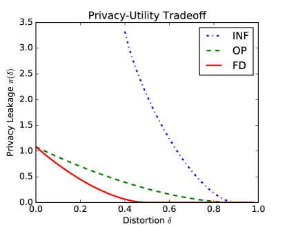
Figure 2: Optimal privacy-utility tradeoff curves under the inference (INF), output perturbation (OP), and full data (FD) scenarios, for the symmetric pair data model with alphabet size $m=10$ and cross-over probability $p=0.4$.

VII Conclusion

In this paper, we formulated the privacy-utility tradeoff problem where the data release mechanism has limited access to the entire data composed of useful and sensitive parts. Based on this information theoretic formulation, we compared the privacy-utility tradeoff regions attained by full data, output perturbation, and inference mechanisms, which have access to the entire data, only useful data, and only sensitive data, respectively.

We first observed that the full data mechanism provides the best privacy-utility tradeoff and then showed that the output perturbation mechanism provides a better privacy-utility tradeoff than the inference mechanism. We showed that if the common and mutual information between useful and sensitive data are identical, then the full data mechanism simplifies to the output perturbation mechanism. Conversely, we showed that if the common information is not equal to mutual information, then the tradeoff region achieved by full data mechanism is strictly larger than the one achieved by the output perturbation mechanism.

Throughout the paper, we allowed for a general distortion measure, and a general privacy measure that satisfies certain conditions that any reasonable measure of privacy should satisfy. In particular, the measure does not have to be symmetric and need not satisfy both the inequalities that are usually implied by the data processing inequality for a symmetric measure. In this context, the linkage inequality was identified as the key property that is required for our main results to hold. It was shown that the Sibson mutual information of order infinity and the information privacy measures satisfy both the post-processing and linkage inequalities, but the maximal information leakage and differential privacy measures can violate the linkage inequality. The philosophical implications of this for differential privacy were also highlighted through a carefully constructed analytical example.

Appendix A Proofs of Section IV Results

A-A Proof of Proposition 1

For $X\to Z_{1}\to Z_{2}$ that form a Markov chain, we have that

$$\min_{z_{1}}H(X|Z_{1}=z_{1}) =\min_{z_{1},z_{2}}H(X|Z_{1}=z_{1},Z_{2}=z_{2})$$

$$\leq\min_{z_{2}}H(X|Z_{1},Z_{2}=z_{2})$$

$$\leq\min_{z_{2}}H(X|Z_{2}=z_{2}),$$

and thus, $I^{*}(X;Z_{1})\geq I^{*}(X;Z_{2})$, establishing the post-processing inequality.

Violation of the linkage inequality is shown by considering the counter-example where $X_{2}$ is ternary with $P_{X_{2}}(0)=1/2$ and $P_{X_{2}}(1)=P_{X_{2}}(2)=1/4$, $X_{1}$ is binary with $X_{1}=0$ if and only if $X_{2}=0$, and the release $Z=X_{1}$. For this example, $X_{2}\to X_{1}\to Z$ is a Markov chain, $I^{*}(X_{1};Z)=H(X_{1})=1$, and $I^{*}(X_{2};Z)=H(X_{2})=1.5$, since $H(X_{1}|Z=0)=H(X_{2}|Z=0)=0$. Hence, $I^{*}(X_{2};Z)>I^{*}(X_{1};Z)$ and the linkage inequality does not hold.

A-B Proof of Lemma 1

Due to symmetry, it suffices to show only the post-processing inequality. For $X\to Z_{1}\to Z_{2}$ that form a Markov chain, we have that

$$IP(X;Z_{2}) =\max_{x,z_{2}}\left|\ln\frac{P_{X|Z_{2}}(x|z_{2})}{P_{X}(x)}\right|$$

$$=\max_{x,z_{2}}\left|\ln\sum_{z_{1}}\frac{P_{X|Z_{1}}(x|z_{1})P_{Z_{1}|Z_{2}}(z_{1}|z_{2})}{P_{X}(x)}\right|$$

$$=\max_{x,z_{2}}\left|\ln E_{Z_{1}}\left[\frac{P_{X|Z_{1}}(x|Z_{1})}{P_{X}(x)}\bigg{|}Z_{2}=z_{2}\right]\right|$$

$$\leq\max_{x,z_{1}}\left|\ln\frac{P_{X|Z_{1}}(x|z_{1})}{P_{X}(x)}\right|=IP(X;Z_{1}),$$

where each maximization is over the supports of the respective marginal distributions, and the inequality follows since the absolute-log of the expectation is bounded by the maximum of the absolute-log over the support.

A-C Proof of Corollary 1

From (8) it follows that

$$IP(X;Z)\leq\max_{\begin{subarray}{c}\mathcal{A}\subseteq\mathcal{X},\mathcal{B}\subseteq\mathcal{Z}:\\ \Pr(X\in\mathcal{A}),\Pr(Z\in\mathcal{B})>0\end{subarray}}\left|\ln\frac{\Pr(X\in\mathcal{A},Z\in\mathcal{B})}{\Pr(X\in\mathcal{A})\Pr(Z\in\mathcal{B})}\right|.$$

To demonstrate the reverse inequality, we first observe that

$$\max_{\begin{subarray}{c}\mathcal{A}\subseteq\mathcal{X},\mathcal{B}\subseteq\mathcal{Z}:\\ \Pr(X\in\mathcal{A}),\Pr(Z\in\mathcal{B})>0\end{subarray}}\left|\ln\frac{\Pr(X\in\mathcal{A},Z\in\mathcal{B})}{\Pr(X\in\mathcal{A})\Pr(Z\in\mathcal{B})}\right|=$$

$$\max_{\begin{subarray}{c}\mathcal{A}\subseteq\mathcal{X},\mathcal{B}\subseteq\mathcal{Z}:\\ \Pr(X\in\mathcal{A}),\Pr(Z\in\mathcal{B})>0\end{subarray}}IP(1(X\in\mathcal{A});1(Z\in\mathcal{B})).$$

Next note that $1(X\in\mathcal{A})\to X\to Z\to 1(Z\in\mathcal{B})$ forms a Markov chain for any choice of $\mathcal{A}\subseteq\mathcal{X},\mathcal{B}\subseteq\mathcal{Z}$ such that $\Pr(X\in\mathcal{A}),\Pr(Z\in\mathcal{B})>0$. From Lemma 1 it follows that $IP(1(X\in\mathcal{A});1(Z\in\mathcal{B}))$ cannot be larger than $IP(X;Z)$ (post-processing and linkage inequalities) for any valid choice of $\mathcal{A,B}$. Thus,

$$\max_{\begin{subarray}{c}\mathcal{A}\subseteq\mathcal{X},\mathcal{B}\subseteq\mathcal{Z}:\\ \Pr(X\in\mathcal{A}),\Pr(Z\in\mathcal{B})>0\end{subarray}}IP(1(X\in\mathcal{A});1(Z\in\mathcal{B}))\leq IP(X;Z)$$

and the result follows.

A-D Proof of Lemma 2

From the definition its follows that a release mechanism is $\epsilon$-differentially private if, and only if, for all $x_{1},x_{2}\in\mathcal{X}$ with $d_{H}(x_{1},x_{2})=1$, and all $\mathcal{B}\subseteq\mathcal{Z}$,

$$\left|\ln\frac{\Pr(Z\in\mathcal{B}|x_{1})}{\Pr(Z\in\mathcal{B}|x_{2})}\right|\leq\epsilon$$

Thus if a release mechanism is $\epsilon$-differentially private, then

$$DP(X;Z):=\max_{\begin{subarray}{c}x_{1},x_{2}\in\mathcal{X},\mathcal{B}\subseteq\mathcal{Z}:\\ d_{H}(x_{1},x_{2})=1\end{subarray}}\left|\ln\frac{\Pr(Z\in\mathcal{B}|x_{1})}{\Pr(Z\in\mathcal{B}|x_{2})}\right|\leq\epsilon.$$ (16)

Since

$$\frac{\Pr(Z\in\mathcal{B}|X=x_{1})}{\Pr(Z\in\mathcal{B}|X=x_{2})}=\frac{\sum_{z\in\mathcal{B}}P_{Z|X}(z|x_{1})}{\sum_{z\in\mathcal{B}}P_{Z|X}(z|x_{2})}\leq\max_{z\in\mathcal{B}}\frac{P_{Z|X}(z|x_{1})}{P_{Z|X}(z|x_{2})},$$

it follows that reducing the scope of maximization in (16) from subsets $\mathcal{B}\subseteq\mathcal{Z}$ to singletons $z\in\mathcal{Z}$ will not decrease the maximum value, i.e.,

A-E Proof of Proposition 2

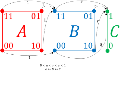
Figure 3: An example which demonstrates that DP can violate the linkage inequality. Here, $A$ and $B$ are databases taking values in $\{0,1\}^{2}$ and $C\in\{0,1\}$ is the data release. The colored edges indicate databases that differ in exactly one element. By construction, $A\to B\to C$ forms a Markov chain and yet $DP(A;C)>DP(B;C)$.

We will construct $A\to B\to C$ such that $DP(A;C)>DP(B;C)$. Let databases $A,B\in\{0,1\}^{2}$ and the release $C\in\{0,1\}$. The database $B:=(B_{1},B_{2})$ is a deterministic function of the database $A:=(A_{1},A_{2})$. Specifically, $B_{1}=B_{2}=A_{1}\vee A_{2}$. The release $C$ is produced by the mechanism $P_{C|B}$, given by

$$P_{C|B}(1|b)=\begin{cases}q,&\text{if }b=(0,0),\\ s,&\text{if }b=(1,1),\\ r,&\text{otherwise},\end{cases}$$

with $0<q<r<s<1$. The construction of $(A,B,C)$ is summarized in Fig. 3 where the solid circles indicate databases and the colored edges join databases that are at Hamming distance one from each other. Since $0<q<r<s<1$,

$$1<\max\left(\frac{s}{r},\frac{r}{q}\right)<\frac{s}{q}$$

If we define $\bar{t}:=(1-t)$ for convenience, then $0<\bar{s}<\bar{r}<\bar{q}<1$ so that

$$1<\max\left(\frac{\bar{r}}{\bar{s}},\frac{\bar{q}}{\bar{r}}\right)<\frac{\bar{q}}{\bar{s}}.$$

Thus,

$$0=\ln 1<DP(B;C) =\max\left(\ln\frac{s}{r},\ln\frac{r}{q},\ln\frac{\bar{q}}{\bar{r}},\ln\frac{\bar{r}}{\bar{s}}\right)$$

$$<\max\left(\ln\frac{s}{q},\ln\frac{\bar{q}}{\bar{s}}\right)=DP(A;C).$$

Appendix B Properties of Common Information

The graphical representation of $P_{X,Y}$ is the bipartite graph with an edge between $x\in\mathcal{X}$ and $y\in\mathcal{Y}$ if and only if $P_{X,Y}(x,y)>0$. The common part $U$ of two random variables $(X,Y)$ is defined as the (unique) label of the connected component of the graphical representation of $P_{X,Y}$ in which $(X,Y)$ falls. Note that $U$ is a deterministic function of $X$ alone and also a deterministic function of $Y$ alone.

The Gács-Körner common information of two random variables $(X,Y)$ is given by entropy of the common part, that is, $C(X;Y):=H(U)$, and has the operational significance of being the maximum number of common bits per symbol that can be independently extracted from $X$ and $Y$ [15]. In general, $C(X;Y)\leq I(X;Y)$, with equality if and only if $X\to U\to Y$ forms a Markov chain [23]. Since our results are only concerned with whether $C(X;Y)=I(X;Y)$, our theorem statements are unchanged if we use instead the Wyner notion of common information (see [14]), since it is also equal to mutual information if and only if $X\to U\to Y$ forms a Markov chain [23].

We give the following lemma which aids our proof of Theorem 3 in Appendix E.

Lemma 4.

If $C(X;Y)\neq I(X;Y)$, then there exist $x_{0},x_{1}\in\mathcal{X}$ and $y_{0},y_{1}\in\mathcal{Y}$, such that $y_{0}\neq y_{1}$, $P_{X,Y}(x_{0},y_{0})>0$, $P_{X,Y}(x_{0},y_{1})>0$, and $P_{X|Y}(x_{1}|y_{0})\neq P_{X|Y}(x_{1}|y_{1})$.

Proof.

We will prove this lemma by showing the contrapositive, that is, if there does not exist $x_{0},x_{1}\in\mathcal{X}$ and $y_{0},y_{1}\in\mathcal{Y}$ satisfying the conditions stated in the lemma, then $C(X;Y)=I(X;Y)$. First, note that if for all $x_{0}\in\mathcal{X}$ and $y_{0},y_{1}\in\mathcal{Y}$, either $y_{0}=y_{1}$, $P_{X,Y}(x_{0},y_{0})=0$, or $P_{X,Y}(x_{0},y_{1})=0$, then $Y$ is a deterministic function of $X$, which would result in $C(X;Y)=I(X;Y)$. Thus, we are left with showing that for all $x_{0}\in\mathcal{X}$ and $y_{0},y_{1}\in\mathcal{Y}$, with $y_{0}\neq y_{1}$, $P_{X,Y}(x_{0},y_{0})>0$, and $P_{X,Y}(x_{0},y_{1})>0$, if we also have that for all $x_{1}\in\mathcal{X}$, $P_{X|Y}(x_{1}|y_{0})=P_{X|Y}(x_{1}|y_{1})$, then $C(X;Y)=I(X;Y)$. This follows since these conditions would imply that for the common part $U$ of $(X,Y)$, $X\to U\to Y$ forms a Markov chain. ∎

Appendix C Proof of Theorem 1

It is sufficient to show that for any mechanism $P_{Z|X}$ that is a feasible solution in the inference optimization of (6), there is a corresponding mechanism $P_{Z^{\prime}|Y}$ for the output perturbation optimization of (5) that achieves the same distortion and only lesser or equal privacy-leakage.

Let $P_{Z|X}$ be a mechanism in the feasible region of the inference optimization problem of (6). Define the corresponding mechanism for the output perturbation optimization of (5) by

$$P_{Z^{\prime}|Y}(z|y):=\sum_{x\in\mathcal{X}}P_{Z|X}(z|x)P_{X|Y}(x|y).$$

Let $(X,Y,Z,Z^{\prime})\sim P_{X,Y}P_{Z|X}P_{Z^{\prime}|Y}$. Note that by construction, $(Y,Z)$ and $(Y,Z^{\prime})$ have the same distribution $P_{Y}P_{Z^{\prime}|Y}$. Thus, both mechanisms achieve the same distortion $D(P_{Y}P_{Z^{\prime}|Y})$ and $J(Y;Z)=J(Y;Z^{\prime})$. Further, by construction, $Y\to X\to Z$ and $X\to Y\to Z^{\prime}$ form Markov chains. Thus, by the linkage inequality,

$$J(X;Z^{\prime})\leq J(Y;Z^{\prime})=J(Y;Z)\leq J(X;Z),$$

showing that the output perturbation mechanism has only lesser or equal privacy-leakage.

Appendix D Proof of Theorem 2

Since $\pi_{\text{FD}}(\delta)\leq\pi_{\text{OP}}(\delta)$ is immediate, we only need to show that $\pi_{\text{OP}}(\delta)\leq\pi_{\text{FD}}(\delta)$. It is sufficient to show that for any mechanism $P_{Z|X,Y}$ that is a feasible solution in the full data optimization of (4), there is a corresponding mechanism $P_{Z^{\prime}|Y}$ for the output perturbation optimization of (5) that achieves the same distortion and only lesser or equal privacy-leakage.

Let $P_{Z|X,Y}$ be a mechanism in the feasible region of the full data optimization problem of (4). Define the corresponding mechanism for the output perturbation optimization of (5) by

$$P_{Z^{\prime}|Y}(z|y):=\sum_{x\in\mathcal{X}}P_{Z|X,Y}(z|x,y)P_{X|Y}(x|y).$$

Let $(X,Y,Z,Z^{\prime})\sim P_{X,Y}P_{Z|X,Y}P_{Z^{\prime}|Y}$, and let $U$ be the common part of $(X,Y)$, where, by construction, $U$ is a deterministic function of either $X$ alone or $Y$ alone. Since $C(X;Y)=I(X;Y)$, we have that $X\to U\to Y$ forms a Markov chain, i.e., $I(X;Y|U)=0$. By construction, $X\to Y\to Z^{\prime}$ also forms a Markov chain, and hence $I(X;Z^{\prime}|U,Y)=I(X;Z^{\prime}|Y)=0$, since $U$ is deterministic function of $Y$. Given these two Markov chains, we have

$$0 =I(X;Y|U)+I(X;Z^{\prime}|U,Y)$$

$$=I(X;Y,Z^{\prime}|U)$$

$$=I(X;Z^{\prime}|U)+I(X;Y|U,Z^{\prime})$$

$$\geq I(X;Z^{\prime}|U),$$

and hence $I(X;Z^{\prime}|U)=0$, i.e., $X\to U\to Z^{\prime}$ also forms a Markov chain. Continuing, we can show the desired privacy-leakage inequality as follows

$$J(X;Z^{\prime}) \leq J(X,U;Z^{\prime})$$

$$\leq J(U;Z^{\prime})$$

$$=J(U;Z)$$

$$\leq J(X,U;Z)$$

$$\leq J(X;Z),$$

where the equality holds since by construction $P_{Y,Z}=P_{Y,Z^{\prime}}$ (and hence $P_{U,Z}=P_{U,Z^{\prime}}$), and the four inequalities follow, respectively, by applying the linkage inequality to the following Markov chains:

• $X\to(X,U)\to Z^{\prime}$, since $X$ is a function of $(X,U)$.

• $(X,U)\to U\to Z^{\prime}$, since $U$ is a function of $X$, and since $X\to U\to Z^{\prime}$ forms a Markov chain as shown above.

• $U\to(X,U)\to Z$, since $U$ is a function of $(X,U)$.

• $(X,U)\to X\to Z$, since $(X,U)$ is a function of $X$.

Appendix E Proof of Theorem 3

We will show the following result, which is key to the proof.

Lemma 5.

If $C(X;Y)\neq I(X;Y)$ then there exist random variables $Z$ and $Z^{\prime}$ with $P_{Y,Z}=P_{Y,Z^{\prime}}$, such that $X\to Y\to Z^{\prime}$ forms a Markov chain, $I(X;Z)=0$, and $I(X;Z^{\prime})>0$.

The proof of Theorem 3 then follows by defining the distortion measure $D(P_{Y,Z})$ to equal $1$ for the particular choice of $P_{Y,Z^{\prime}}$ in Lemma 5 and to equal $2$ otherwise, and choosing $\delta=1$. This choice for the distortion measure and distortion level restricts the feasible output perturbation mechanism to only $P_{Z^{\prime}|Y}$, which by Lemma 5 results in $\pi_{OP}(\delta)>0$ since $J(X;Z^{\prime})>0$ (since $I(X;Z^{\prime})>0$). However, the proof of Lemma 5 (see below) also ensures the existence of $Z$ produced by a full data mechanism $P_{Z|X,Y}$ that results in $\pi_{FD}(\delta)=0$ since $I(X;Z)=0$.

Using the symbols $(x_{0},x_{1},y_{0},y_{1})$ shown to exist by Lemma 4, we can prove Lemma 5 by constructing a binary $Z$ with alphabet $\mathcal{Z}=\{0,1\}$ as follows. Choose any $s\in(0,1)$ and any $t\in\left(0,\min\{s^{\prime}/P_{Y|X}(y_{1}|x_{0}),s/P_{Y|X}(y_{0}|x_{0})\}\right)$, where $s^{\prime}:=(1-s)$. Define $Z$ with $(X,Y,Z)\sim P_{X,Y}P_{Z|X,Y}$, where

$$P_{Z|X,Y}(0|x,y):=\begin{cases}s+tP_{Y|X}(y_{1}|x_{0}),&\text{if }(x,y)=(x_{0},y_{0}),\\ s-tP_{Y|X}(y_{0}|x_{0}),&\text{if }(x,y)=(x_{0},y_{1}),\\ s,&\text{otherwise}.\end{cases}$$

The choice of $s$ and $t$ ensures that $P_{Z|X,Y}(0|x,y)\in(0,1)$ for all $(x,y)\in\mathcal{X}\times\mathcal{Y}$. This construction of $P_{Z|X,Y}$ makes $Z$ independent of $X$, since for all $x\in\mathcal{X}$ in the support of $P_{X}$,

$$P_{Z|X}(0|x)=\sum_{y\in\mathcal{Y}}P_{Z|X,Y}(0|x,y)P_{Y|X}(y|x)=s.$$

With the above construction, we have

$$P_{Z|Y}(0|y) =\sum_{x\in\mathcal{X}}P_{Z|X,Y}(0|x,y)P_{X|Y}(x|y)$$

$$=\begin{cases}s+tP_{Y|X}(y_{1}|x_{0})P_{X|Y}(x_{0}|y_{0}),&\text{if }y=y_{0},\\ s-tP_{Y|X}(y_{0}|x_{0})P_{X|Y}(x_{0}|y_{1}),&\text{if }y=y_{1},\\ s,&\text{otherwise}.\end{cases}$$

Next, we construct binary $Z^{\prime}$ such that $X\to Y\to Z^{\prime}$ forms a Markov chain, with $(X,Y,Z^{\prime})\sim P_{X,Y}P_{Z^{\prime}|Y}$, where we set $P_{Z^{\prime}|Y}:=P_{Z|Y}$. Then, consider

$$P_{Z^{\prime}|X}(0|x) =\sum_{y\in\mathcal{Y}}P_{Z^{\prime}|Y}(0|y)P_{Y|X}(y|x)$$

$$=\sum_{y\in\mathcal{Y}}P_{Z|Y}(0|y)P_{Y|X}(y|x)$$

$$=s+tP_{Y|X}(y_{1}|x_{0})P_{X|Y}(x_{0}|y_{0})P_{Y|X}(y_{0}|x)$$

$$\quad\quad-tP_{Y|X}(y_{0}|x_{0})P_{X|Y}(x_{0}|y_{1})P_{Y|X}(y_{1}|x)$$

$$=s+tP_{X}(x_{0})P_{Y|X}(y_{0}|x_{0})P_{Y|X}(y_{1}|x_{0})$$

$$\quad\quad\times[P_{X|Y}(x|y_{0})-P_{X|Y}(x|y_{1})]/P_{X}(x).$$

Finally, we show that $P_{Z^{\prime}|X}(0|x)$ is not constant for all $x\in\mathcal{X}$ in the support of $P_{X}$, which implies that $Z^{\prime}$ is not independent of $X$, i.e., $I(X;Z^{\prime})>0$. This can be proved by contradiction, by supposing that $P_{Z^{\prime}|X}(0|x)$ is constant for all $x\in\mathcal{X}$ in the support of $P_{X}$. Then, for all $x\in\mathcal{X}$,

$$P_{X|Y}(x|y_{0})-P_{X|Y}(x|y_{1})=cP_{X}(x),$$

for some constant $c$. By summing over all $x\in\mathcal{X}$, we have that $c=0$. This would imply that $P_{X|Y}(x|y_{0})=P_{X|Y}(x|y_{1})$ for all $x\in\mathcal{X}$, contradicting the existence of $x_{1}\in\mathcal{X}$ given by Lemma 4 for the choice of $y_{0}$ and $y_{1}$.

Appendix F Some Useful Lemmas

In this section, we provide a set of lemmas that we use to prove the results presented in Section VI.

Lemma 6.

Let $X,Y$, and $Z$ be discrete random variables, with $X,Y\in\{0,\dots,m-1\}$. If $(X,Y)\sim SP(m,p)$, then

$$\Pr(Y\neq Z)-\Pr(X\neq Z)$$

$$\quad=\frac{p}{m(m-1)}\mathop{\sum_{x,y}}_{x\neq y}\left[P_{Z|X,Y}(x|x,y)-P_{Z|X,Y}(y|x,y)\right]$$

Proof.

We can expand $\Pr(Y\neq Z)$ as

$$\Pr(Y\neq Z) =1-\Pr(Y=Z)$$

$$=1-\sum_{x,y}P_{X,Y}(x,y)P_{Z|X,Y}(y|x,y)$$

$$=1-\sum_{x}P_{X,Y}(x,x)P_{Z|X,Y}(x|x,x)$$

$$\quad-\sum_{x\neq y}P_{X,Y}(x,y)P_{Z|X,Y}(y|x,y)$$

$$=1-\frac{1-p}{m}\sum_{x}P_{Z|X,Y}(x|x,x)$$

$$\quad-\frac{p}{m(m-1)}\sum_{x\neq y}P_{Z|X,Y}(y|x,y).$$

Similarly, we have that

$$P(X\neq Z) =1-\frac{1-p}{m}\sum_{x}P_{Z|X,Y}(x|x,x)$$

$$\quad-\frac{p}{m(m-1)}\sum_{x\neq y}P_{Z|X,Y}(x|x,y).$$

Subtracting these two expansions yields the lemma. ∎

Lemma 7.

Let $X,Y$, and $Z$ be discrete random variables, with $X,Y\in\{0,\dots,m-1\}$. If $(X,Y)\sim SP(m,p)$ and $Y\to X\to Z$ forms a Markov chain, then

$$\Pr(Y\neq Z)=p+\Pr(X\neq Z)\left(1-\frac{pm}{m-1}\right).$$

Proof.

We have that

$$\Pr(Y\neq Z)-\Pr(X\neq Z)$$

$$\quad\stackrel{{\scriptstyle(a)}}{{=}}\frac{p}{m(m-1)}\mathop{\sum_{x,y}}_{x\neq y}P_{Z|X,Y}(x|x,y)-P_{Z|X,Y}(y|x,y)$$

$$\quad\stackrel{{\scriptstyle(b)}}{{=}}\frac{p}{m(m-1)}\mathop{\sum_{x,y}}_{x\neq y}P_{Z|X}(x|x)-P_{Z|X}(y|x)$$

$$\quad\stackrel{{\scriptstyle(c)}}{{=}}\frac{p}{(m-1)}\mathop{\sum_{x,y}}_{x\neq y}P_{X,Z}(x,x)-P_{X,Z}(x,y)$$

$$\quad=\frac{p}{(m-1)}((m-1)\Pr(X=Z)-P(X\neq Z))$$

$$\quad=p-\Pr(X\neq Z)\left(p+\frac{p}{m-1}\right),$$

where (a) follows from Lemma 6, (b) since $Y\to X\to Z$ forms a Markov chain, and (c) since $X$ is uniform over $\{0,\dots,m-1\}$. Rearranging terms yields the lemma. ∎

Lemma 8.

Let $X$ be uniformly distributed on $\{0,\dots,m-1\}$ and define

$$f(\epsilon):= \inf_{P_{Z|X}}I(X;Z)$$

$$\ \ \text{s.t.}\ \Pr(X\neq Z)\leq\epsilon,$$

and

$$g(\epsilon):=\begin{cases}r_{m}(\epsilon),&\text{if }\epsilon\leq 1-\frac{1}{m}\\ 0,&\text{otherwise},\end{cases}$$

for $\epsilon\in[0,\infty)$. Then, $f(\epsilon)$ = $g(\epsilon)$ for any $\epsilon\in[0,\infty)$, with the mechanism $P_{Z|X}$ solving the optimization problem given by

$$P_{Z|X}(z|x)=\begin{cases}{1-t},\text{ if }z=x\\ \frac{t}{m-1},\text{ otherwise,}\end{cases}$$ (17)

where $t:=\min(1-\frac{1}{m},\epsilon)$ and $z\in\{0,\dots,m-1\}$.

Proof.

We immediately have that $f(\epsilon)=g(\epsilon)=0$ for any $\epsilon>1-\frac{1}{m}$, since for $Z$ independent of $X$ and uniformly distributed over $\{0,\ldots,m-1\}$, which is consistent with (17), we have that $\Pr(X\neq Z)=1-\frac{1}{m}$ and $I(X;Z)=0$. Thus, for the rest of the proof, we assume that $\epsilon\leq 1-\frac{1}{m}$.

We first show that $f(\epsilon)\geq g(\epsilon)$, using a lower bound on $I(X;Z)$,

$$I(X;Z) =\log m-H(X|Z)$$

$$\geq r_{m}(\Pr(X\neq Z)),$$ (18)

which follows from Fano’s inequality and definition of $r_{m}$ from Lemma 3. Thus, for $\epsilon\leq 1-\frac{1}{m}$,

$$f(\epsilon) \geq\inf_{P_{Z|X}}r_{m}(\Pr(X\neq Z))\quad\text{s.t. }\Pr(X\neq Z)\leq\epsilon$$

$$=r_{m}(\epsilon)=:g(\epsilon),$$

since $r_{m}(\epsilon)$ is strictly decreasing over $[0,1-\frac{1}{m}]$.

We next show that $f(\epsilon)\leq g(\epsilon)$ for $P_{Z|X}$ given by (17). Note that $(X,Z)\sim SP(m,t)$, and hence the conditional probability $P_{Z|X}$ is in the feasible region of the optimization problem since $\Pr(X\neq Z)=t=\epsilon$. Consequently, we have $f(\epsilon)\leq I(X;Z)=r_{m}(t)=g(\epsilon)$, where the first equality follows from Lemma 3 and the second since $t=\epsilon\leq 1-\frac{1}{m}$. ∎

Lemma 9.

Let $X$ be uniformly distributed on $\{0,\dots,m-1\}$ and define

$$f^{*}(\epsilon):= \inf_{P_{Z|X}}I(X;Z)$$

$$\ \ \text{s.t.}\ \Pr(X\neq Z)\geq\epsilon,$$

and

$$g^{*}(\epsilon):=\begin{cases}r_{m}(\epsilon),&\text{if }\epsilon\geq 1-\frac{1}{m}\\ 0,&\text{otherwise},\end{cases}$$

for $\epsilon\in[0,1]$. Then, $f^{*}(\epsilon)$ = $g^{*}(\epsilon)$ for any $\epsilon\in[0,1]$, with the mechanism $P_{Z|X}$ solving the optimization problem given by (17) with $t:=\max(1-\frac{1}{m},\epsilon)$.

Proof.

We immediately have that $f^{*}(\epsilon)=g^{*}(\epsilon)=0$ for any $\epsilon<1-\frac{1}{m}$, since for $Z$ independent of $X$ and uniformly distributed over $\{0,\ldots,m-1\}$, which is consistent with (17) with $t:=\max(1-\frac{1}{m},\epsilon)$, we have that $\Pr(X\neq Z)=1-\frac{1}{m}$ and $I(X;Z)=0$. Thus, for the rest of the proof, we assume that $\epsilon\geq 1-\frac{1}{m}$.

We first show that $f^{*}(\epsilon)\geq g^{*}(\epsilon)$, applying the lower bound of (18) to yield

$$f^{*}(\epsilon) \geq\inf_{P_{Z|X}}r_{m}(\Pr(X\neq Z))\quad\text{s.t. }\Pr(X\neq Z)\geq\epsilon$$

$$=r_{m}(\epsilon)=:g^{*}(\epsilon),$$

which follows since $r_{m}(\epsilon)$ is strictly increasing over $[1-\frac{1}{m},1]$.

We next show that $f^{*}(\epsilon)\leq g^{*}(\epsilon)$ for $P_{Z|X}$ given by (17) with $t:=\max(1-\frac{1}{m},\epsilon)$. Note that $(X,Z)\sim SP(m,t)$, and hence the conditional probability $P_{Z|X}$ is in the feasible region of the optimization problem since $\Pr(X\neq Z)=t=\epsilon$. Consequently, we have $f(\epsilon)\leq I(X;Z)=r_{m}(t)=g(\epsilon)$, where the first equality follows from Lemma 3 and the second since $t=\epsilon\geq 1-\frac{1}{m}$. ∎

Appendix G Proof of Theorem 4

For convenience, we define

$$g_{\text{FD}}(\delta):=\begin{cases}r_{m}(p+\delta),&\text{if }\delta\leq 1-\frac{1}{m}-p,\\ r_{m}(p-\delta),&\text{if }\delta\leq p-(1-\frac{1}{m}),\\ 0,&\text{otherwise}.\end{cases}$$

which is equal to the right-hand side of (11). Since, for $\delta\geq 1-\frac{1}{m}$, we immediately have $g_{\text{FD}}(\delta)=\pi_{\text{FD}}(\delta)=0$, we will assume that $\delta<1-\frac{1}{m}$ for the rest of this proof.

We divide the proof into two cases: (i) $p\leq 1-\frac{1}{m}$ and (ii) $p>1-\frac{1}{m}$.

Case 1: $p\leq 1-\frac{1}{m}$

We first show that $\pi_{\text{FD}}(\delta)\geq g_{\text{FD}}(\delta)$. Due to Lemma 6, we have that $\Pr(Y\neq Z)\leq\delta$ implies that

$$\Pr(X\neq Z)\leq\delta$$

$$\quad\quad+\frac{p}{m(m-1)}\mathop{\sum_{x,y}}_{x\neq y}\left[P_{Z|X,Y}(y|x,y)-P_{Z|X,Y}(x|x,y)\right],$$

$$\quad\leq\delta+\frac{p}{m(m-1)}\mathop{\sum_{x,y}}_{x\neq y}1$$

$$\quad\leq\delta+p,$$

Thus, for any mechanism $P_{Z|X,Y}$ with $\Pr(Y\neq Z)\leq\delta$, we have that $\Pr(X\neq Z)\leq\delta+p$. Then, we bound $\pi_{\text{FD}}(\delta)$ via

$$\pi_{\text{FD}}(\delta) \geq\inf_{P_{Z|X,Y}}I(X;Z)\quad\text{s.t. }\Pr(X\neq Z)\leq\delta+p$$

$$=\inf_{P_{Z|X}}I(X;Z)\quad\text{s.t. }\Pr(X\neq Z)\leq\delta+p$$

$$=g_{\text{FD}}(\delta),$$

where the last equality follows from Lemma 8.

We next show that $\pi_{\text{FD}}(\delta)\leq g_{\text{FD}}(\delta)$ via the mechanism given by (12), which is feasible since

$$\Pr(Y\neq Z) =\Pr(Y\neq Z|X=Y)\Pr(X=Y)$$

$$=\Pr(N\neq 0|X=Y)(1-p)$$

$$=t\leq\delta.$$

Hence, we have that $\pi_{\text{FD}}(\delta)\leq I(X;Z)$. For all $x\neq z$, we have that

$$P_{X,Z}(x,z) =\sum_{y}P_{Z|X,Y}(z|x,y)P_{X,Y}(x,y)$$

$$=P_{Z|X,Y}(z|x,x)P_{X,Y}(x,x)$$

$$\quad+\sum_{y\neq x}P_{Z|X,Y}(z|x,y)P_{X,Y}(x,y)$$

$$=\frac{t}{(1-p)(m-1)}\frac{1-p}{m}+P_{X,Y}(x,z)$$

$$=\frac{t}{(m-1)m}+\frac{p}{(m-1)m}$$

$$=\frac{t+p}{(m-1)m},$$

which shows that $(X,Z)\sim SP(m,t+p)$. Thus, by Lemma 3, $I(X;Z)=r_{m}(t+p)$. Noting that $r_{m}(1-\frac{1}{m})=0$, we have $r_{m}(t+p)=g_{\text{FD}}(\delta)$ for $p\leq 1-\frac{1}{m}$. Hence, $\pi_{\text{FD}}(\delta)\leq g_{\text{FD}}(\delta)$.

Case 2: $p>1-\frac{1}{m}$

We first show that $\pi_{\text{FD}}(\delta)\geq g_{\text{FD}}(\delta)$. Given $\Pr(Y\neq Z)\leq\delta$, we have that

$$\Pr(X\neq Z)+\delta \geq\Pr(X\neq Z)+\Pr(Y\neq Z)$$

$$\geq\Pr(\{X\neq Z\}\cup\{Y\neq Z\})$$

$$=1-\Pr(X=Y=Z)$$

$$\geq 1-\Pr(X=Y)$$

$$=p.$$

Thus, for any mechanism $P_{Z|X,Y}$ that satisfies $\Pr(Y\neq Z)\leq\delta$, we also have that $\Pr(X\neq Z)\geq p-\delta$. Then, we can bound $\pi_{\text{FD}}(\delta)$ via

$$\pi_{\text{FD}}(\delta) \geq\inf_{P_{Z|X,Y}}I(X;Z)\quad\text{s.t. }\Pr(X\neq Z)\geq p-\delta$$

$$=\inf_{P_{Z|X}}I(X;Z)\quad\text{s.t. }\Pr(X\neq Z)\geq p-\delta$$

$$=g_{\text{FD}}(\delta),$$

where the last equality follows from Lemma 9.

We next show $\pi_{\text{FD}}(\delta)\leq g_{\text{FD}}(\delta)$, by considering the mechanism defined by

$$Z:=\begin{cases}Y,&\text{if }\theta^{\prime}=1,\\ X,&\text{otherwise},\end{cases}$$

where $\theta^{\prime}$ is a binary random variable that is independent of $(X,Y)$, with $\Pr(\theta^{\prime}=1)=t^{\prime}/p$, where we define $t^{\prime}:=\max(p-\delta,1-\frac{1}{m})$ for convenience. Since

$$\Pr(Y\neq Z) =\Pr(Y\neq Z|\theta^{\prime}=0)P_{\theta^{\prime}}(0)$$

$$=\Pr(Y\neq X|\theta^{\prime}=0)P_{\theta^{\prime}}(0)$$

$$=\Pr(Y\neq X)P_{\theta^{\prime}}(0)$$

$$=p-t^{\prime}$$

$$\leq\delta,$$

we have that this mechanism is feasible. Hence, we have $\pi_{\text{FD}}(\delta)\leq I(X;Z)$. For all $x\neq z$, we have that

$$P_{X,Z}(x,z) =\sum_{y}P_{Z|X,Y}(z|x,y)P_{X,Y}(x,y)$$

$$=P_{Z|X,Y}(z|x,x)P_{X,Y}(x,x)$$

$$\quad+\sum_{y\neq x}P_{Z|X,Y}(z|x,y)P_{X,Y}(x,y)$$

$$=0+P_{Z|X,Y}(z|x,z)P_{X,Y}(x,z)+0$$

$$=\frac{t^{\prime}}{p}\frac{p}{(m-1)m}$$

$$=\frac{t^{\prime}}{(m-1)m},$$

which shows that $(X,Z)\sim SP(m,t^{\prime})$. Thus, by Lemma 3, $I(X;Z)=r_{m}(t^{\prime})$. Noting that $r_{m}(1-\frac{1}{m})=0$, we have $r_{m}(t^{\prime})=g_{\text{FD}}(\delta)$ for all $p\geq 1-\frac{1}{m}$. Hence, $\pi_{\text{FD}}(\delta)\leq g_{\text{FD}}(\delta)$.

Appendix H Proof of Theorem 5

For convenience, we define

$$g_{\text{OP}}(\delta):=\begin{cases}r_{m}\left(p+\delta\left(1-\frac{pm}{m-1}\right)\right),&\text{if }\delta<1-\frac{1}{m},\\ 0,&\text{otherwise}.\end{cases}$$

which is equal to the right-hand side of (13). Since, for $\delta\geq 1-\frac{1}{m}$, we immediately have $g_{\text{OP}}(\delta)=\pi_{\text{OP}}(\delta)=0$, we will assume that $\delta<1-\frac{1}{m}$ for the rest of this proof.

We first show that $\pi_{\text{OP}}(\delta)\geq g_{\text{OP}}(\delta)$. Since $X\to Y\to Z$ forms a Markov chain for any output perturbation mechanism, we have from Lemma 7 that

$$\Pr(X\neq Z)=p+\Pr(Y\neq Z)\left(1-\frac{pm}{m-1}\right).$$

Let $\delta^{\prime}:=p+\delta\left(1-\frac{pm}{m-1}\right)$. Note that when $p\leq 1-\frac{1}{m}$, the term $\left(1-\frac{pm}{m-1}\right)\geq 0$. Hence, the constraint $\Pr(Y\neq Z)\leq\delta$ is equivalent to $\Pr(X\neq Z)\leq\delta^{\prime}$, and $\delta^{\prime}<1-\frac{1}{m}$ since $\delta<1-\frac{1}{m}$. Thus, for $p\leq 1-\frac{1}{m}$, we can bound $\pi_{\text{OP}}(\delta)$ via

$$\pi_{\text{OP}}(\delta) =\inf_{P_{Z|Y}}I(X;Z)\quad\text{s.t. }\Pr(X\neq Z)\leq\delta^{\prime}$$

$$\geq\inf_{P_{Z|X}}I(X;Z)\quad\text{s.t. }\Pr(X\neq Z)\leq\delta^{\prime}$$

$$=g_{\text{OP}}(\delta),$$

where the inequality is due to the removal of the Markov chain constraint and the final equality follows from Lemma 8. The case when $p>1-\frac{1}{m}$ follows similarly, except now the term $\left(1-\frac{pm}{m-1}\right)<0$, hence the constraint $\Pr(Y\neq Z)\leq\delta$ is equivalent to $\Pr(X\neq Z)\geq\delta^{\prime}$, and $\delta^{\prime}>1-\frac{1}{m}$. Thus, for $p>1-\frac{1}{m}$, we can bound $\pi_{\text{OP}}(\delta)$ via

$$\pi_{\text{OP}}(\delta) =\inf_{P_{Z|Y}}I(X;Z)\quad\text{s.t. }\Pr(X\neq Z)\geq\delta^{\prime}$$

$$\geq\inf_{P_{Z|X}}I(X;Z)\quad\text{s.t. }\Pr(X\neq Z)\geq\delta^{\prime}$$

$$=g_{\text{OP}}(\delta),$$

where the inequality is due to the removal of the Markov chain constraint and the final equality follows from Lemma 9.

We next show that $\pi_{\text{OP}}(\delta)\leq g_{\text{OP}}(\delta)$, via the mechanism given by $Z:=Y+N\mod m$, where $N$ is independent of $(X,Y)$, and distributed according to (14). This mechanism is feasible since $\Pr(Y\neq Z)=t:=\min(\delta,1-\frac{1}{m})\leq\delta$. Hence, we have $\pi_{\text{OP}}(\delta)\leq I(X;Z)$. For all $x\neq z$, we have that

$$P_{X,Z}(x,z)=\sum_{y}P_{Z|Y}(z|y)P_{X,Y}(x,y)$$

$$\quad=P_{Z|Y}(z|z)P_{X,Y}(x,z)+\sum_{y\neq z}P_{Z|Y}(z|y)P_{X,Y}(x,y)$$

$$\quad=(1-t)P_{X,Y}(x,z)$$

$$\quad\quad+\frac{t}{(m-1)}\left(P_{X,Y}(x,x)+\sum_{y\notin\{x,z\}}P_{X,Y}(x,y)\right)$$

$$\quad=\frac{(1-t)p}{(m-1)m}+\frac{t}{(m-1)}\left(\frac{(1-p)}{m}+\frac{p(m-2)}{(m-1)m}\right)$$

$$\quad=\frac{p+t\left(1-\frac{pm}{m-1}\right)}{(m-1)m}$$

$$\quad=:\frac{\delta^{\prime\prime}}{(m-1)m}$$

which shows that $(X,Z)\sim SP(m,\delta^{\prime\prime})$. Thus, by Lemma 3, $I(X;Z)=r_{m}(\delta^{\prime\prime})$. Noting that $r_{m}(1-\frac{1}{m})=0$, we have $r_{m}(\delta^{\prime\prime})=g_{\text{OP}}(\delta)$. Hence, $\pi_{\text{OP}}(\delta)\leq g_{\text{OP}}(\delta)$.

Appendix I Proof of Theorem 6

For convenience, we define

$$g_{\text{INF}}(\delta):=\begin{cases}r_{m}(t),&\text{if }\delta<1-\frac{1}{m}\text{ and }p\notin(\delta,h),\\ \infty,&\text{if }\delta<1-\frac{1}{m}\text{ and }p\in(\delta,h),\\ 0,&\text{if }\delta\geq 1-\frac{1}{m},\end{cases}$$

which is equal to the right-hand side of (15), where $h:=(m-1)(1-\delta)$ and

$$t:=\frac{\delta-p}{1-\frac{pm}{m-1}}.$$

Since, for $\delta\geq 1-\frac{1}{m}$, we immediately have $g_{\text{INF}}(\delta)=\pi_{\text{INF}}(\delta)=0$, we will assume that $\delta<1-\frac{1}{m}$ for the rest of this proof. Note that with this assumption, we have $h>1-\frac{1}{m}$.

Since $Y\to X\to Z$ forms a Markov chain for any inference mechanism, we have from Lemma 7 that

$$\Pr(Y\neq Z)=p+\Pr(X\neq Z)\left(1-\frac{pm}{m-1}\right).$$

Note that if $p=1-\frac{1}{m}$, then $\Pr(Y\neq Z)=1-\frac{1}{m}>\delta$, and the optimization is infeasible, hence $g_{\text{INF}}(\delta)=\pi_{\text{INF}}(\delta)=\infty$. Thus, we will consider the two remaining cases: (i) $p<1-\frac{1}{m}$ and (ii) $p>1-\frac{1}{m}$.

Case 1: $p<1-\frac{1}{m}$

In this case, we have that the constraint $\Pr(Y\neq Z)\leq\delta$ is equivalent to

$$\Pr(X\neq Z)\leq\frac{\delta-p}{1-\frac{mp}{m-1}}=:t,$$

due to Lemma 7. For $p>\delta$, the optimization problem is infeasible since $t<0$, and hence $g_{\text{INF}}(\delta)=\pi_{\text{INF}}(\delta)=\infty$. Otherwise, for $p\leq\delta$, we have that $0\leq t\leq 1-\frac{1}{m}$, and by Lemma 8, we have that $g_{\text{INF}}(\delta)=\pi_{\text{INF}}(\delta)=r_{m}(t)$.

Case 2: $p>1-\frac{1}{m}$

In this case, we have that the constraint $\Pr(Y\neq Z)\leq\delta$ is equivalent to

$$\Pr(X\neq Z)\geq\frac{\delta-p}{1-\frac{pm}{m-1}}=:t,$$

due to Lemma 7 and since the denominator is negative. For $p<h$, the optimization problem is infeasible since $t>1$, and hence $g_{\text{INF}}(\delta)=\pi_{\text{INF}}(\delta)=\infty$. Otherwise, for $p\geq h$, we have that $1-\frac{1}{m}\leq t\leq 1$, and by Lemma 9, we have that $g_{\text{INF}}(\delta)=\pi_{\text{INF}}(\delta)=r_{m}(t)$.

References

• [1] Y. O. Basciftci, Y. Wang, and P. Ishwar, “On privacy-utility tradeoffs for constrained data release mechanisms,” in Information Theory and Applications Workshop, Feb. 2016.
• [2] D. Rebollo-Monedero, J. Forné, and J. Domingo-Ferrer, “From t-closeness-like privacy to postrandomization via information theory,” IEEE Trans. Knowl. Data Eng., vol. 22, no. 11, pp. 1623–1636, 2010.
• [3] L. Sweeney, “Simple demographics often identify people uniquely,” Carnegie Mellon University, Data Privacy Working Paper, 2000.
• [4] A. Narayanan and V. Shmatikov, “Robust de-anonymization of large sparse datasets,” in IEEE Symp. on Security and Privacy.   IEEE, 2008, pp. 111–125.
• [5] L. Sweeney, “k-anonymity: A model for protecting privacy,” Intl. Journal of Uncertainty, Fuzziness and Knowledge-Based Systems, vol. 10, no. 5, pp. 557–570, 2002.
• [6] A. Machanavajjhala, D. Kifer, J. Gehrke, and M. Venkitasubramaniam, “l-diversity: Privacy beyond k-anonymity,” ACM Trans. on Knowledge Discovery from Data, vol. 1, no. 1, p. 3, 2007.
• [7] N. Li, T. Li, and S. Venkatasubramanian, “t-closeness: Privacy beyond k-anonymity and l-diversity,” in IEEE Intl. Conf. on Data Eng.   IEEE, 2007, pp. 106–115.
• [8] C. Dwork, F. McSherry, K. Nissim, and A. Smith, “Calibrating noise to sensitivity in private data analysis,” in Theory of Cryptography.   Springer, 2006, pp. 265–284.
• [9] F. du Pin Calmon and N. Fawaz, “Privacy against statistical inference,” in Allerton Conf. on Comm., Ctrl., and Comp., 2012, pp. 1401–1408.
• [10] H. Yamamoto, “A source coding problem for sources with additional outputs to keep secret from the receiver or wiretappers,” IEEE Trans. on Information Theory, vol. 29, no. 6, pp. 918–923, 1983.
• [11] L. Sankar, S. R. Rajagopalan, and H. V. Poor, “Utility-privacy tradeoffs in databases: An information-theoretic approach,” IEEE Trans. on Information Forensics and Security, vol. 8, no. 6, pp. 838–852, 2013.
• [12] I. Issa, S. Kamath, and A. B. Wagner, “An operational measure of information leakage,” in Information Science and Systems (CISS), 2016, pp. 234–239.
• [13] D. Kifer and B.-R. Lin, “An axiomatic view of statistical privacy and utility,” Journal of Privacy and Confidentiality, vol. 4, no. 1, pp. 5–49, 2012.
• [14] A. Wyner, “The common information of two dependent random variables,” IEEE Transactions on Information Theory, vol. 21, no. 2, pp. 163–179, Mar. 1975.
• [15] P. Gács and J. Körner, “Common information is far less than mutual information,” Problems of Control and Information Theory, vol. 2, no. 2, pp. 149–162, 1973.
• [16] H. S. Witsenhausen, “Indirect rate distortion problems,” IEEE Transactions on Information Theory, vol. 26, no. 5, pp. 518–521, 1980.
• [17] N. Tishby, F. C. Pereira, and W. Bialek, “The information bottleneck method,” in Allerton Conf. on Comm., Ctrl., and Comp., 1999, pp. 368––377.
• [18] T. M. Cover and J. A. Thomas, Elements of information theory, 2nd ed.   John Wiley & Sons, 2012.
• [19] A. Makhdoumi, S. Salamatian, N. Fawaz, and M. Médard, “From the information bottleneck to the privacy funnel,” in IEEE Information Theory Workshop, 2014, pp. 501–505.
• [20] R. Sibson, “Information radius,” Zeitschrift für Wahrscheinlichkeitstheorie und verwandte Gebiete, vol. 14, no. 2, pp. 149–160, 1969.
• [21] D. Kifer and A. Machanavajjhala, “No free lunch in data privacy,” in Proceedings of the 2011 ACM SIGMOD International Conference on Management of data.   ACM, 2011, pp. 193–204.
• [22] C. Liu, S. Chakraborty, and P. Mittal, “Dependence makes you vulnberable: Differential privacy under dependent tuples,” in Network and Distributed System Security Symposium, 2016.
• [23] R. Ahlswede and J. Körner, “On common information and related characteristics of correlated information sources,” in Proc. Prague Conf. on Information Theory, 1974.