Phenomenology of neutron-antineutron conversion

Abstract

We consider the possibility of neutron-antineutron ($n-{\bar{n}}$) conversion, in which the change of a neutron into an antineutron is mediated by an external source, as can occur in a scattering process. We develop the connections between $n-{\bar{n}}$ conversion and $n-{\bar{n}}$ oscillation, in which a neutron spontaneously tranforms into an antineutron, noting that if $n-{\bar{n}}$ oscillation occurs in a theory with B-L violation, then $n-{\bar{n}}$ conversion can occur also. We show how an experimental limit on $n-{\bar{n}}$ conversion could connect concretely to a limit on $n-{\bar{n}}$ oscillation, and vice versa, using effective field theory techniques and baryon matrix elements computed in the M.I.T. bag model.

I Introduction

Establishing that the symmetry of baryon number minus lepton number, B-L, is broken in nature would demonstrate that dynamics beyond the standard model (SM) exists. This prospect is often discussed in the context of the origin of the neutrino mass, with B-L violation necessary both to make neutrinoless double $\beta$ (0$\nu\beta\beta$) decay possible and to give the neutrino a Majorana mass weinberg1979baryon ; schechter1982neutrino . The would-be mechanism of 0$\nu\beta\beta$ decay is unknown, so that it need not be realized through the long-range exchange of a Majorana neutrino, nor need it even utilize neutrinos at all — yet its observation would imply the neutrino has a Majorana mass schechter1982neutrinoless . In this paper we discuss the complementary possibility of B-L violation in the quark sector mohapatra1980local ; mohapatra1980phenomenology , and we develop new pathways to its discovery through the consideration of $n$-${\bar{n}}$ conversion.

We draw a distinction between an $n$-${\bar{n}}$ oscillation kuzmin1970zhetf ; Glashow1979 ; mohapatra1980local , in which the neutron would spontaneously transforms into an antineutron with the same energy and momentum, and an $n$-${\bar{n}}$ conversion, in which the neutron would transform into an antineutron as mediated by an external source. The ability to observe $n$-${\bar{n}}$ oscillations is famously fragile and can disappear in the presence of ordinary matter and magnetic fields Glashow1979 ; mohapatra1980phenomenology ; cowsik1981some . Such environmental effects impact the neutron and antineutron differently, in that the energies of a neutron and antineutron are no longer the same, so that one particle cannot convert spontaneously into the other and satisfy energy-momentum conservation, a constraint that unbroken Lorentz symmetry demands. It is technically possible, but experimentally involved, to remove matter and magnetic fields to the extent that sensitive experimental searches with free neutrons become possible. The most recent, and most sensitive, of such experimental searches was completed more than twenty years ago baldo1994new , yielding a $n\bar{n}$ lifetime limit of $\tau_{n\bar{n}}=0.85\times 10^{8}\,\hbox{s}$ at 90% confidence level (CL). A next-generation experiment is also under development phillips2016neutron ; milstead2015new . Independently, searches for neutron-antineutron oscillations in nuclei have been conducted, with the most stringent lower limit on the bound neutron lifetime being $1.9\times 10^{32}$ years at 90% CL for neutrons in ¹⁶O Abe:2011ky . Employing a probabilistic computation of the nuclear suppression factor Dover:1982wv ; Friedman:2008es , with realistic nuclear optical potentials Friedman:2008es , yields an equivalent free neutron lifetime of $2.7\times 10^{8}\,\hbox{s}$ at 90% CL Abe:2011ky . A recent study of the bound neutron lifetime in deuterium Aharmim:2017jna also employs a probabilistic framework Kopeliovich:2011aa to determine that the equivalent free neutron lifetime is no less than $1.23\times 10^{8}$ s at 90% CL. We note that the ability of the free neutron experiment to observe a non-zero effect at its claimed sensitivity has been recently called into question Kerbikov:2017spv , due to the use of a probabilistic, rather than a quantum kinetic, framework for its analysis. We thus find it of particular interest to explore pathways to B-L violation for which these limitations do not apply.

In this paper, we consider how it may be possible to observe B-L violation with baryons without requiring that a neutron spontaneously oscillates into an antineutron. One alternate path, that of dinucleon decay in nuclei Mohapatra:1982eu ; kabir1983limits ; basecq1983deltab ; arnold2013simplified , is known and is being actively studied berger1991lifetime ; bernabei2000search ; litos2014search ; gustafson2015search , though its sensitivity is limited by the finite density of bound nuclei. Another possibility occurs if the neutron transforms into an antineutron while coupling to an external vector current, as possible in a scattering process. The latter is not sensitive to the presence of matter and magnetic fields, because the external current permits energy-momentum conservation to be satisfied irrespective of such effects. As we shall see, the leading-dimension effective operators that realize this are of higher mass dimension than those that give rise to $n$-${\bar{n}}$ oscillations, or dinucleon decay; however, the difference in mass dimension need not be compensated by a new physics mass scale — and thus the amplitude for an $n$-${\bar{n}}$ conversion need not be much smaller than that for an $n$-${\bar{n}}$ oscillation. Moreover, since the neutron is a composite of quarks, and the quarks carry both electric and color charge, operators that mediate $n$-${\bar{n}}$ oscillations can be related to those that generate $n$-${\bar{n}}$ conversion. To make our discussion concrete, we consider the example of electron-neutron scattering, so that $n$-${\bar{n}}$ conversion would be mediated by the electromagnetic current, though free neutron targets are not practicable. Rather, an “effective” neutron target such as ²H or ³He would be needed, though the neutron absorption cross section on ³He is too large to make that choice practicable. The reactions of interest would thus include $e+^{2}\!{\rm H}\to e+{\bar{n}}+X(n,p)$, or, alternatively, either $n+e\to{\bar{n}}+e$ or $n+^{2}\!{\rm H}\to{\bar{n}}+p+X(e)$, where $X(n,p)$, e.g., denotes an unspecified final state containing a neutron and a proton. Studies with heavier nuclei, generally $n+A\to{\bar{n}}+X(n,p)$, with $A$ denoting a nucleus such as ⁵⁸Ni, could also be possible.

The observation of an $n$-${\bar{n}}$ transition would speak to new physics at the TeV scale, and particular model realizations contain not only TeV-scale new physics but also give neutrinos suitably-sized Majorana masses mohapatra1980local ; chacko1999supersymmetric ; babu2001observable . However, proving that the neutrino has a Majorana mass in the absence of the observation of 0$\nu\beta\beta$ decay requires not only an observation of B-L violation, but also that of another baryon number violating process babu2015determining . Improving the experimental limit on the non-appearance of $n$-${\bar{n}}$ oscillations can also severely constrain particular models of baryogenesis babu2009neutrino ; babu2012coupling ; babu2013post . It could also help shed light on the mechanism of 0$\nu\beta\beta$ decay in nuclei, which could arise from a short-distance mechanism mediated by TeV-scale, B-L violating new physics or a long-range exchange of a Majorana neutrino, with new physics appearing, rather, at much higher energy scales, as the supposed mechanism of 0$\nu\beta\beta$ decay. The continued non-appearence of neutron-antineutron oscillations and thus of TeV-scale physics may ultimately speak in favor of a light Majorana neutrino mechanism for 0$\nu\beta\beta$ decay.

In this paper we develop the possibility of $n-{\bar{n}}$ conversion in a concrete way. We begin, in Sec. II, by constructing an low-energy, effective Lagrangian in neutron and antineutron degrees of freedom with B-L violation, in which the hadrons also interact with electromagnetic fields or sources. It has been common to analyze the sensitivity to $n-{\bar{n}}$ oscillations within an effective Hamiltonian framework mohapatra1980phenomenology ; we employ its spin-dependent version gardner2015 to show how the spin dependence of $n-{\bar{n}}$ conversion leaves the transition probability unsuppressed in the presence of a magnetic field. To redress the possibility of suppression from matter effects, however, a different experimental concept is needed unless the matter were removed — we refer to Ref. Kerbikov:2017spv for a discussion of the implied experimental requirements. We develop the possibility of $n-{\bar{n}}$ conversion through scattering in Sec. III. Here our particular interest is how it might be connected theoretically to the possibility of $n$-${\bar{n}}$ oscillation. We do this by working at an energy scale high enough to resolve the quarks in the hadrons; thus to realize $n-{\bar{n}}$ conversion we start with the quark-level operators that mediate $n-{\bar{n}}$ oscillation and dress the quarks with photons to enable electromagnetic scattering. With this we find the quark-level operators that mediate $n-{\bar{n}}$ conversion. In Sec. IV we compute the matching conditions to the hadron-level effective theory, computing the needed matrix elements in the M.I.T. bag model Chodos:1974pn ; Chodos:1974je . This gives us a concrete connection between $n-{\bar{n}}$ conversion and oscillation. Finally in Sec. VI we analyze the efficacy of different experimental pathways to produce $n-{\bar{n}}$ conversion, and particularly the best indirect limit on $n-{\bar{n}}$ oscillation parameters, and we conclude with a summary and outlook in Sec. VII. In a separate paper we develop how best to discover $n$-${\bar{n}}$ conversion in its own right svgxy_search17 .

II Low-energy $n$-${\bar{n}}$ transitions with spin

At low-energy scales we can regard neutrons and antineutrons as effectively elementary particles and realize $n-\bar{n}$ transitions through B-L violating effective operators in these degrees of freedom. Previously we have shown that the unimodular phases associated with the discrete symmetry transformations of Dirac fermions must be restricted in the presence of B-L violation; particularly, we have found that the phase associated with CPT must be imaginary gardner2016c . We refer the reader to Appendix A for a summary of our definitions and conventions. The notion that Majorana particles, being their own antiparticles, have special transformation properties under CPT, CP, and C is long known, as are their implications for the interpretation of 0$\nu\beta\beta$ experiments Kayser:1983wm ; Kayser:1984ge . More generally, the existence of phase constraints associated with the discrete symmetry transformations of Majorana fields had already been noted by Feinberg and Weinberg Feinberg:1959 , as well as by Carruthers Carruthers:1971 , with these authors determining the phase restrictions associated with the C, CP, T, and TP transformations. Haxton and Stephenson Haxton:1985am have also analyzed the phase constraint associated with C for a pseudo-Dirac neutrino Wolfenstein:1981kw , the case most similar to that of the neutron, though they did not analyze the phase constraints associated with the other discrete symmetries. Under our CPT phase constraint, there are two leading mass dimension, CPT even and Lorentz invariant, $n-\bar{n}$ transition operators, namely, ${\cal O}_{1}=n^{T}Cn+{\rm h.c.}$ and ${\cal O}_{2}=n^{T}C\gamma_{5}n+{\rm h.c.}$ A third operator appears if we admit an interaction with an external vector current $j^{\mu}$ berev15 : ${\cal O}_{3}=n^{T}C\gamma^{\mu}\gamma_{5}nj_{\mu}+{\rm h.c.}$ Note that a B-L-violating interaction of form $in^{T}C\not{\partial}n+{\rm h.c.}$ vanishes under the use of the equation of motion for a free Dirac field. With this in hand, we find that the effective Lagrangian of $n-\bar{n}$ conversion, mediated through electromagnetic interactions, is

$${\mathcal{L}}_{\rm eff}=i{\bar{n}}{\not{\partial}}n-M{\bar{n}}n-\frac{1}{2}\mu_{n}{\bar{n}}\sigma^{\mu\nu}nF_{\mu\nu}-\frac{\delta}{2}(n^{T}Cn+{\rm h.c.})-\frac{\eta}{2}(n^{T}C\gamma^{\mu}\gamma^{5}nj_{\mu}+{\rm{h.c.}})\,,$$ (1)

where $n$ denotes the neutron field with mass $M$ and magnetic moment $\mu_{n}$, $j^{\mu}$ is the current associated with a spin 1/2 particle with electromagnetic charge $Qe$, noting $F^{\mu\nu}$ is the electromagnetic tensor, and $\delta$ and $\eta$ are real constants. Using Maxwell equations with Heaviside-Lorentz conventions, we can replace the current $j^{\nu}\equiv\bar{\psi}\gamma^{\nu}\psi$ with fields via $Qej^{\nu}=\partial_{\mu}F^{\mu\nu}$ as convenient. We have neglected the possibility of a $n^{T}C\gamma_{5}n+{\rm h.c.}$ term, although CPT and Lorentz symmetry permits it gardner2016c , because it does not contribute to $n-{\bar{n}}$ oscillations gardner2015 ; berev15 ; Fujikawa:2016sft . The presence of the external current $j^{\mu}$ makes $n-{\bar{n}}$ transitions with a flip of spin possible. To illustrate the efficacy of this, we now turn to the computation of the $n-{\bar{n}}$ transition probability in the presence of a non-uniform magnetic field.

To compute the transition probability in an effective Hamiltonian framework with spin degrees of freedom gardner2015 , we must work out the $4\times 4$ mass matrix ${\cal M}$ associated with Eq. (1). Using the $i\in|n(\mathbf{p},+)\rangle$, $|{\bar{n}}(\mathbf{p},+)\rangle$, $|{n}(\mathbf{p},-)\rangle$, $|{\bar{n}}(\mathbf{p},-)\rangle$ basis with $\mathbf{p}=0$, we compute the matrix elements of the Hamiltonian $H$ associated with $\mathcal{L}_{\rm eff}$ and define the elements of ${\cal M}$ so that ${\cal M}_{ij}=\langle i|H|j\rangle/2M$. Evaluating ${\cal M}_{ij}$ explicitly, we note that matrix elements associated with the $\eta$-dependent term are spin dependent. Although magnetic fields do act to suppress $n-\bar{n}$ oscillations mediated by the $\delta$ term in $\mathcal{L}_{\rm eff}$, the behavior of the $\eta$-dependent term is different. Suppose a magnetic field $\mathbf{B}$ is present. We choose the spin quantization axis so that $\mathbf{S}$ is aligned with $\mathbf{B}$ and the $\hat{\mathbf{z}}$ axis. Defining $\omega_{0}\equiv|\boldsymbol{\mu}_{n}||\mathbf{B}|$ and $\boldsymbol{\omega}\equiv\eta\mathbf{j}$ with $Qej^{\nu}=\partial_{\mu}F^{\mu\nu}$, we find

$$\mathcal{M}=\begin{pmatrix}M+\omega_{0}&\delta+\omega_{z}&0&\omega_{x}-i\omega_{y}\\ \delta+\omega_{z}&M-\omega_{0}&\omega_{x}-i\omega_{y}&0\\ 0&\omega_{x}+i\omega_{y}&M-\omega_{0}&\delta-\omega_{z}\\ \omega_{x}+i\omega_{y}&0&\delta-\omega_{z}&M+\omega_{0}\end{pmatrix}\,,$$ (2)

where we have assumed that $\mathbf{j}$ and $\mathbf{B}$ are roughly constant. If $\mathbf{B}$ is non-uniform and depends on the transverse coordinates $x$ and $y$, then $\omega_{x}$ and $\omega_{y}$ can both be non-zero, whereas $\omega_{z}$ will vanish in the absence of an electric field. Introducing $\omega_{xy}=\sqrt{\omega_{x}^{2}+\omega_{y}^{2}}$, we solve for the eigenvalues and eigenvectors of Eq. (2) (with $\omega_{z}=0$) to determine the probability that an neutron with spin $s=+$ transforms into an antineutron with $s=\pm$. We find

$${\cal P}_{n+\rightarrow\bar{n}+} = \frac{\delta^{2}}{\delta^{2}+\omega_{0}^{2}}\sin^{2}(t\sqrt{\delta^{2}+\omega_{0}^{2}})\cos^{2}(t\omega_{xy})\approx\frac{\delta^{2}}{\omega_{0}^{2}}\sin^{2}t\omega_{0}\,,$$ (3)

$${\cal P}_{n+\rightarrow\bar{n}-} = \sin^{2}(t\omega_{xy})\left(\cos^{2}(t\sqrt{\delta^{2}+\omega_{0}^{2}})+\frac{\omega_{0}^{2}}{\delta^{2}+\omega_{0}^{2}}\sin^{2}(t\sqrt{\delta^{2}+\omega_{0}^{2}})\right)\approx\sin^{2}(t\omega_{xy})\,,$$ (4)

where the approximate result reports the probability to leading order in B-L violation. We observe that $\mathcal{P}_{n+\rightarrow\bar{n}+}$ is quenched by the magnetic field, in that it becomes negligibly small unless $t\omega_{0}\ll 1$, which is not surprising since the spin is not flipped. In contrast, $\mathcal{P}_{n+\rightarrow\bar{n}-}$ is not suppressed. Although we have illustrated the utility of the $j^{\mu}$ term in a particular case, our conclusion holds more generally. In particular, we can probe $n$-${\bar{n}}$ conversion through a scattering process, so that the neutron and antineutron do not have to have the same energy and momentum. Consequently, we are no longer bound to the context of an oscillation framework, and the quenching problems arising from the presence of either matter or magnetic fields are completely solved. For future reference we note that free $n-{\bar{n}}$ searches are conducted in the so-called quasifree limit, so that Eq. (3) can be approximated by $\delta^{2}t^{2}$. Thus a limit on the free $n{\bar{n}}$ lifetime $\tau_{n\bar{n}}$ corresponds to a limit on $\delta$ via $\delta=\tau_{n\bar{n}}^{-1}$, so that the limit from the ILL experiment can be expressed as $\delta\leq 5\times 10^{-32}\,\hbox{GeV}$ at 90% CL baldo1994new .

In what follows we develop how limits from low-energy scattering experiments that would search for $n$-${\bar{n}}$ transitions can connect concretely to limits from $n$-${\bar{n}}$ oscillation searches. Before so doing, we note that a oscillation search after the manner of existing experiments baldo1994new could also set a limit on $\eta$ directly by utilizing non-uniform or non-stationary electromagnetic fields to generate a nonzero $\omega_{xy}$ svgxy_search17 .

III $n$-${\bar{n}}$ transition operators at the quark level

Considering the $n$-${\bar{n}}$ transition operators of Eq. (1) from the viewpoint of simple dimensional analysis, we see that the mass dimension of $\delta$, $[\delta]$, has $[\delta]=1$, whereas $[\eta]=-2$ since $[j^{\mu}]=3$. Since $[\eta/\delta]=-3$, one might think that $n-\bar{n}$ conversion would be suppressed by an additional factor of $\Lambda_{NP}^{3}$, where $\Lambda_{NP}$ is the cutoff mass scale of new physics. This is not necessarily true because of the presence of other energy scales. To illustrate this explicitly, we need to develop the form of the $n-\bar{n}$ conversion operators at the quark-level. We do this by considering energy scales at which the quark structure of the nucleon becomes explicit but are still well below the nominal scale of new physics, $\Lambda_{\rm QCD}\lesssim E\ll\Lambda_{\rm NP}$. In this way we can realize quark-level $n$-${\bar{n}}$ conversion operators through electromagnetic interactions, by dressing the quarks of the quark-level $n-\bar{n}$ oscillation operators with photons, since the participating quarks also carry electric charge.

The effective Lagrangian for $n-\bar{n}$ oscillations at the QCD scale involves operators with six quark fields, and which thus have an associated coefficient of mass dimension ${-5}$. Since these operators are key to our work, we briefly summarize their important ingredients. Based on our earlier discussion of the nucleon-level operators, we expect the quark-level “building blocks” to have the structure $q^{T\alpha}_{1\,\chi}Cq^{\beta}_{2\,\chi}$, where the numerical and Greek indices are flavor and color labels, respectively. We work, too, in a chiral basis with $\chi\in{\rm L,R}$ and note that each quark block appears as a chiral pair, since operators of mixed chirality always vanish. The final $n$-${\bar{n}}$ operators should be compatible with the hadrons’ flavor content and also be invariant under color symmetry, SU(3)_c. There are three ways of forming an SU(3) singlet from a product of six fundamental representations in SU(3)_c. However, in the case of quarks of a single generation, only two color tensors can occur Rao:1983sd , namely,

$$(T_{s})_{\alpha\beta\gamma\delta\rho\sigma} = \epsilon_{\rho\alpha\gamma}\epsilon_{\sigma\beta\delta}+\epsilon_{\sigma\alpha\gamma}\epsilon_{\rho\beta\delta}+\epsilon_{\rho\beta\gamma}\epsilon_{\sigma\alpha\delta}+\epsilon_{\sigma\beta\gamma}\epsilon_{\rho\alpha\delta}\,,$$ (5)

$$(T_{a})_{\alpha\beta\gamma\delta\rho\sigma} = \epsilon_{\rho\alpha\beta}\epsilon_{\sigma\gamma\delta}+\epsilon_{\sigma\alpha\beta}\epsilon_{\rho\gamma\delta}\,$$ (6)

with $\epsilon$ denoting a totally antisymmetric tensor. We refer to Ref. Rao:1983sd for a discussion of B-L violating operators with arbitrary generational structure. Working in a chiral basis, so that $q_{\chi}\equiv(1+{\chi}\gamma_{5})q/2$ and $\chi=\pm$ (or, equivalently, writing $q_{\chi}$ with $\chi={\stackrel{{\scriptstyle R}}{{{}_{L}}}}$), we note, ultimately, that there are three types of $n$-${\bar{n}}$ operators Rao:1982gt :

$$(\mathcal{O}_{1})_{\chi_{1}\chi_{2}\chi_{3}} = [u^{T\alpha}_{\chi_{1}}Cu^{\beta}_{\chi_{1}}][d^{T\gamma}_{\chi_{2}}Cd^{\delta}_{\chi_{2}}][d^{T\rho}_{\chi_{3}}Cd^{\sigma}_{\chi_{3}}](T_{s})_{\alpha\beta\gamma\delta\rho\sigma},$$ (7)

$$(\mathcal{O}_{2})_{\chi_{1}\chi_{2}\chi_{3}} = [u^{T\alpha}_{\chi_{1}}Cd^{\beta}_{\chi_{1}}][u^{T\gamma}_{\chi_{2}}Cd^{\delta}_{\chi_{2}}][d^{T\rho}_{\chi_{3}}Cd^{\sigma}_{\chi_{3}}](T_{s})_{\alpha\beta\gamma\delta\rho\sigma},$$ (8)

$$(\mathcal{O}_{3})_{\chi_{1}\chi_{2}\chi_{3}} = [u^{T\alpha}_{\chi_{1}}Cd^{\beta}_{\chi_{1}}][u^{T\gamma}_{\chi_{2}}Cd^{\delta}_{\chi_{2}}][d^{T\rho}_{\chi_{3}}Cd^{\sigma}_{\chi_{3}}](T_{a})_{\alpha\beta\gamma\delta\rho\sigma}\,,$$ (9)

although only 14 of these 24 operators are independent, because the antisymmetric tensors yield the relationships Rao:1982gt

$$(\mathcal{O}_{1})_{\chi_{1}LR}=(\mathcal{O}_{1})_{\chi_{1}RL}\,,\ \ (\mathcal{O}_{2,3})_{LR\chi_{3}}=(\mathcal{O}_{2,3})_{RL\chi_{3}}\,,$$ (10)

and Caswell:1982qs

$$(\mathcal{O}_{2})_{mmn}-(\mathcal{O}_{1})_{mmn}=3(\mathcal{O}_{3})_{mmn}\,,$$ (11)

where $m,n\in[L,R]$. If we also demand that the operators be invariant under SU(2)${}_{L}\times$U(1)_Y, the electroweak gauge symmetry of the SM, then finally only four operators are independent Rao:1982gt ; Caswell:1982qs . For example,

$$\mathscr{P}_{1}=(\mathcal{O}_{1})_{RRR},$$ (12)

$$\mathscr{P}_{2}=(\mathcal{O}_{2})_{RRR},$$ (13)

$$\mathscr{P}_{3}=[q^{Ti\alpha}_{L}Cq^{j\beta}_{L}][u^{T\gamma}_{R}Cd^{\delta}_{R}][d^{T\rho}_{R}Cd^{\sigma}_{R}]\epsilon_{ij}(T_{s})_{\alpha\beta\gamma\delta\rho\sigma}$$

$$\ \ \ \ \ =2(\mathcal{O}_{3})_{LRR}\,,$$ (14)

$$\mathscr{P}_{4}=[q^{Ti\alpha}_{L}Cq^{j\beta}_{L}][q^{Tk\gamma}_{L}Cq^{l\delta}_{L}][d^{T\rho}_{R}Cd^{\sigma}_{R}]\epsilon_{ij}\epsilon_{kl}(T_{a})_{\alpha\beta\gamma\delta\rho\sigma}$$

$$\ \ \ \ \ =4(\mathcal{O}_{3})_{LLR}\,,$$ (15)

where the Roman indices label the members of a left-handed SU(2) doublet.

The matrix elements of these operators have been evaluated in the M.I.T. bag model by Rao and Shrock Rao:1982gt and, much more recently, in lattice QCD Buchoff:2012bm ; Syritsyn:2016ijx . Once we have developed the quark-level $n$-${\bar{n}}$ conversion operators we, too, use the M.I.T. bag model to evaluate their matrix elements. We discuss noteworthy technical aspects of this in Appendix B.

III.1 From quark-level operators for $n$-${\bar{n}}$ oscillation to $n$-${\bar{n}}$ conversion

Since dimensional analysis shows that the effective operator for $n$-${\bar{n}}$ conversion would be suppressed with respect to that for $n$-${\bar{n}}$ oscillation by three powers of a new-physics mass scale, we wish to explore the manner in which we can use SM physics to find a more favorable relationship. In particular, since the quarks carry electric charge, we explore the possibility that the external source in the $n$-${\bar{n}}$ conversion operator is the electromagnetic current. Of course quarks also carry color charge, but the associated current $\partial^{\mu}F_{\mu\nu}^{a}$ is not SU(3)_c gauge invariant. In what follows we consider each of the $n$-${\bar{n}}$ transition operators in turn and determine the low-energy effective operator that follows from evaluating how its quarks interact with a virtual photon generated by a scattered charged particle, such as an electron. In any particular, leading-dimension $n$-${\bar{n}}$ operator, there are three blocks, and in each block there are two charged particles. When a virtual photon is attached to these blocks, there are six possible ways that correspond to six different Feynman diagrams, as shown in Fig. 1. Note that we do not attach a photon line to the solid “blob” at the center because, as we shall see, this would yield an effect that would be suppressed by higher powers of the new physics mass scale.

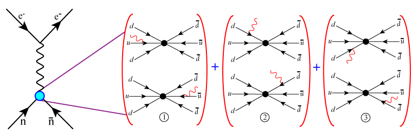
Figure 1: A neutron-antineutron transition is realized through electron-neutron scattering. The virtual photon emitted from the scattered electron interacts with a general six-fermion $n-\bar{n}$ oscillation vertex. The particular graphs showns illustrate the two possible ways of attaching a photon to each of the blocks that appear in the $({\cal O}_{1})_{\chi_{1}\chi_{2}\chi_{3}}$ operator of Eq. (7).

To determine the operator structures that emerge upon including electromagnetic interactions, we first compute the matrix element for the process $q^{\rho}(p)+\gamma(k)\to\bar{q}^{\delta}(p^{\prime})$, noting that the superscripts are flavor indices. Working in a chiral basis, the pertinent terms in the interaction Hamiltonian are

$${\cal H}_{I}\supset\frac{\delta_{q}}{2}\sum_{\chi_{1}}(\psi^{\rho\,T}_{\chi_{1}}C\psi^{\delta}_{\chi_{1}}+{\bar{\psi}}^{\delta}_{\chi_{1}}C{\bar{\psi}}^{\rho\,T}_{\chi_{1}})+Q_{\rho}e\sum_{\chi_{2}}\bar{\psi}_{\chi_{2}}^{\rho}\not{A}\psi_{\chi_{2}}^{\rho}+Q_{\delta}e\sum_{\chi_{3}}\bar{\psi}_{\chi_{3}}^{\delta}\not{A}\psi_{\chi_{3}}^{\delta}\,,$$ (16)

where both $q^{\rho}$ and ${\bar{q}}^{\delta}$ have mass $m$. Computing

$$\langle{\bar{q}}^{\delta}(p^{\prime})|\mathcal{T}\left(\sum_{\chi_{1},\chi_{2}}\left(-i\frac{\delta_{q}}{2}\int d^{4}x\psi^{\rho\,T}_{\chi_{1}}C\psi^{\delta}_{\chi_{1}}\right)\left(-iQ_{\rho}e\int d^{4}y\bar{\psi}_{\chi_{2}}^{\rho}\not{A}\psi_{\chi_{2}}^{\rho}-iQ_{\delta}e\int d^{4}y\bar{\psi}_{\chi_{2}}^{\delta}\not{A}\psi_{\chi_{2}}^{\delta}\right)\right)|q^{\rho}(p)\gamma(k)\rangle\,,$$ (17)

using standard techniques Peskin:1995ev , noting $\mathcal{T}$ is the time-ordering operator and the quarks are treated as free fields, we find

$$-\frac{\delta_{q}}{2}emi\sum_{\chi_{2}}\left(Q_{\rho}\frac{{\bar{u}}^{\delta}(\mathbf{p}^{\prime},s^{\prime})\not{\epsilon}(k)(1+\chi_{2}\gamma_{5})u^{\rho}(\mathbf{p},s)}{{p^{\prime}}^{2}-m^{2}}-Q_{\delta}\frac{{\bar{v}}^{\rho}(\mathbf{p},s)\not{\epsilon}(k)(1+\chi_{2}\gamma_{5})v^{\delta}(\mathbf{p}^{\prime},s^{\prime})}{p^{2}-m^{2}}\right)(2\pi)^{4}\delta^{(4)}(p^{\prime}-p-k)\,,$$ (18)

where $\epsilon_{\mu}$ is the polarization vector of the photon, or, finally,

$$-\frac{\delta_{q}}{2}emi\sum_{\chi_{2}} \Bigg{(}{\bar{u}}^{\delta}(\mathbf{p}^{\prime},s^{\prime})\not{\epsilon}(k)u^{\rho}(\mathbf{p},s)\left(\frac{Q_{\rho}}{{p^{\prime}}^{2}-m^{2}}-\frac{Q_{\delta}}{{p}^{2}-m^{2}}\right)$$ (19)

$$+\chi_{2}{\bar{u}}^{\delta}(\mathbf{p}^{\prime},s^{\prime})\not{\epsilon}(k)\gamma_{5}u^{\rho}(\mathbf{p},s)\left(\frac{Q_{\rho}}{{p^{\prime}}^{2}-m^{2}}+\frac{Q_{\delta}}{{p}^{2}-m^{2}}\right)\Bigg{)}(2\pi)^{4}\delta^{(4)}(p^{\prime}-p-k)$$

where we have employed the conventions and relationships of Appendix A throughout. Since $p^{2}=p^{\prime\,2}$, we see the vector term vanishes if $Q_{\rho}=Q_{\delta}$, as we would expect from CPT considerations gardner2016c . However, if $Q_{\delta}\neq Q_{\rho}$ the final result is non-zero even after summing over $\chi_{2}$. Replacing $\epsilon_{\mu}(k)$ with $k_{\mu}$ we see that the Ward-Takahashi identity is satisfied after summing over $\chi_{2}$. For fixed $\chi_{2}$ the identity also follows once we sum over the photon-quark contributions that would yield an electrically neutral initial or final state, as in the case of $n-{\bar{n}}$ transitions. Thus we extract the effective operator associated with the quark-antiquark-photon vertex as

$$-\frac{m\delta_{q}e}{p^{2}-m^{2}}\left(Q_{\rho}\psi^{\delta\,T}_{-\chi_{2}}C\gamma^{\mu}\psi^{\rho}_{\chi_{2}}-Q_{\delta}\psi^{\delta\,T}_{\chi_{2}}C\gamma^{\mu}\psi^{\rho}_{-\chi_{2}}\right)\,,$$ (20)

noting that only the $C\gamma^{\mu}\gamma_{5}$ Lorentz structure would survive if $\rho=\delta$. For use in the neutron case we recast this as

$$-\frac{m\delta_{q}e}{p^{2}-m^{2}}\left(Q_{\rho}\psi^{\delta\,T}_{-\chi}C\gamma^{\mu}\gamma_{5}\psi^{\rho}_{\chi}+Q_{\delta}\psi^{\delta\,T}_{\chi}C\gamma^{\mu}\gamma_{5}\psi^{\rho}_{-\chi}\right)\,,$$ (21)

so that a sum over $\chi$ would yield the $C\gamma^{\mu}\gamma_{5}$ Lorentz structure that appeared in our neutron-level analysis. Since we plan to study the $\chi$ dependence of the $n$-${\bar{n}}$ conversion operator matrix elements, we may make this replacement without loss of generality. Studying the $\chi$ dependence reveals the interplay of the $C\gamma^{\mu}$ and $C\gamma^{\mu}\gamma_{5}$ Lorentz structures at the quark level, just as studying the $\chi_{1}$, $\chi_{2}$, and $\chi_{3}$ dependence of the $n$-${\bar{n}}$ oscillation matrix elements shows the interplay of $C$ and $C\gamma_{5}$ Lorentz structures, although only $C$ appears in the neutron-level analysis. Since the quark is on its mass shell, we also have $p^{2}=m^{2}$, so that the explicit factor of $1/(p^{2}-m^{2})$ is problematic. However, the process we have computed ought not occur because it does not conserve electric charge. Rather, it may occur within a composite operator for which there is no change in electric charge, so that the participating quarks appear as part of a hadron state. Indeed the phenomenon of confinement in QCD reveals that quarks are never free, so that $p^{2}-m^{2}$ does not vanish in the realistic case. We shall revisit its precise evaluation once the complete $n-{\bar{n}}$ conversion operator is in place.

We can now proceed with our explicit construction of the $n$-${\bar{n}}$ conversion operator associated with $({\cal O}_{1})_{\chi_{1}\chi_{2}\chi_{3}}$ in Eq. (7), for which the pertinent Feynman graphs appear in Fig. 1. Using the effective vertex in Eq. (21) for the two-quark-field-photon block, we see that the enumerated sets of graphs, ①, ②, and ③, correspond to the effective vertices

$$\frac{-2e\delta_{q}}{3}\frac{m}{p^{2}-m^{2}}[u^{\alpha\,T}_{-\chi}C\gamma^{\mu}\gamma_{5}u^{\beta}_{\chi}+u^{\alpha\,T}_{\chi}C\gamma^{\mu}\gamma_{5}u^{\beta}_{-\chi}][d^{\gamma\,T}_{\chi_{2}}Cd^{\delta}_{\chi_{2}}][d^{\rho\,T}_{\chi_{3}}Cd^{\sigma}_{\chi_{3}}](T_{s})_{\alpha\beta\gamma\delta\rho\sigma}\,,$$ (22)

$$\frac{+e\delta_{q}}{3}\frac{m}{p^{2}-m^{2}}[u^{\alpha\,T}_{\chi_{1}}Cu^{\beta}_{\chi_{1}}][d^{\gamma\,T}_{-\chi}C\gamma^{\mu}\gamma_{5}d^{\delta}_{\chi}+d^{\gamma\,T}_{\chi}C\gamma^{\mu}\gamma_{5}d^{\delta}_{-\chi}][d^{\rho\,T}_{\chi_{3}}Cd^{\sigma}_{\chi_{3}}](T_{s})_{\alpha\beta\gamma\delta\rho\sigma}\,,$$ (23)

and

$$\frac{+e\delta_{q}}{3}\frac{m}{p^{2}-m^{2}}[u^{\alpha\,T}_{\chi_{1}}Cu^{\beta}_{\chi_{1}}][d^{\gamma\,T}_{\chi_{2}}Cd^{\delta}_{\chi_{2}}][d^{\rho\,T}_{-\chi}C\gamma^{\mu}\gamma_{5}d^{\sigma}_{\chi}+d^{\rho\,T}_{\chi}C\gamma^{\mu}\gamma_{5}d^{\sigma}_{-\chi}](T_{s})_{\alpha\beta\gamma\delta\rho\sigma}\,,$$ (24)

respectively. Combining these vertices gives the effective operator generated from $({\cal O}_{1})_{\chi_{1}\chi_{2}\chi_{3}}$, namely,

$$(\tilde{\mathcal{O}}_{1})^{\chi\,\mu}_{\chi_{1}\chi_{2}\chi_{3}} = \Big{[}-2[u^{\alpha\,T}_{-\chi}C\gamma^{\mu}\gamma_{5}u^{\beta}_{\chi}+u^{\alpha\,T}_{\chi}C\gamma^{\mu}\gamma_{5}u^{\beta}_{-\chi}][d^{\gamma\,T}_{\chi_{2}}Cd^{\delta}_{\chi_{2}}][d^{\rho\,T}_{\chi_{3}}Cd^{\sigma}_{\chi_{3}}]$$ (25)

$$+ [u^{\alpha\,T}_{\chi_{1}}Cu^{\beta}_{\chi_{1}}][d^{\gamma\,T}_{-\chi}C\gamma^{\mu}\gamma_{5}d^{\delta}_{\chi}+d^{\gamma\,T}_{\chi}C\gamma^{\mu}\gamma_{5}d^{\delta}_{-\chi}][d^{\rho\,T}_{\chi_{3}}Cd^{\sigma}_{\chi_{3}}]$$

$$+ [u^{\alpha\,T}_{\chi_{1}}Cu^{\beta}_{\chi_{1}}][d^{\gamma\,T}_{\chi_{2}}Cd^{\delta}_{\chi_{2}}][d^{\rho\,T}_{-\chi}C\gamma^{\mu}\gamma_{5}d^{\sigma}_{\chi}+d^{\rho\,T}_{\chi}C\gamma^{\mu}\gamma_{5}d^{\sigma}_{-\chi}]\Big{]}(T_{s})_{\alpha\beta\gamma\delta\rho\sigma}\,.$$

Finally, including the current term $Qej^{\mu}(q)/q^{2}$ that appears through electromagnetic scattering, we have the effective $n-\bar{n}$ conversion operator

$$(\tilde{\mathcal{O}}_{1})^{\chi}_{\chi_{1}\chi_{2}\chi_{3}}=(\delta_{1})_{\chi_{1}\chi_{2}\chi_{3}}\frac{em}{3(p_{\rm eff}^{2}-m^{2})}\frac{Qej_{\mu}}{q^{2}}(\tilde{\mathcal{O}}_{1})^{\chi\,\mu}_{\chi_{1}\chi_{2}\chi_{3}}\,,$$ (26)

where $(\delta_{1})_{\chi_{1}\chi_{2}\chi_{3}}$ is the explicit low-energy constant associated with the $({\cal O}_{1})_{\chi_{1}\chi_{2}\chi_{3}}$ operator and we replace $p^{2}\to p_{\rm eff}^{2}$ for clarity in later use. We now turn to the $n$-${\bar{n}}$ conversion operators associated with the other $n$-${\bar{n}}$ operators, $({\mathcal{O}}_{2})_{\chi_{1}\chi_{2}\chi_{3}}$ and $({\mathcal{O}}_{3})_{\chi_{1}\chi_{2}\chi_{3}}$ in Eqs. (8-9). Although the block structure of these operators is quite different from $({\cal O}_{1})_{\chi_{1}\chi_{2}\chi_{3}}$, determining the effective operators is nevertheless straightforward. Employing Eq. (21) for the structure of each two-quark-photon block we find for the effective operator generated from $({\cal O}_{2})_{\chi_{1}\chi_{2}\chi_{3}}$:

$$(\tilde{\mathcal{O}}_{2})^{\chi\,\mu}_{\chi_{1}\chi_{2}\chi_{3}} = \Big{[}[u^{\alpha\,T}_{-\chi}C\gamma^{\mu}\gamma_{5}d^{\beta}_{\chi}-2u^{\alpha\,T}_{\chi}C\gamma^{\mu}\gamma_{5}d^{\beta}_{-\chi}][u^{\gamma\,T}_{\chi_{2}}Cd^{\delta}_{\chi_{2}}][d^{\rho\,T}_{\chi_{3}}Cd^{\sigma}_{\chi_{3}}]$$ (27)

$$+ [u^{\alpha\,T}_{\chi_{1}}Cd^{\beta}_{\chi_{1}}][u^{\gamma\,T}_{-\chi}C\gamma^{\mu}\gamma_{5}d^{\delta}_{\chi}-2u^{\gamma\,T}_{\chi}C\gamma^{\mu}\gamma_{5}d^{\delta}_{-\chi}][d^{\rho\,T}_{\chi_{3}}Cd^{\sigma}_{\chi_{3}}]$$

$$+ [u^{\alpha\,T}_{\chi_{1}}Cd^{\beta}_{\chi_{1}}][u^{\gamma\,T}_{\chi_{2}}Cd^{\delta}_{\chi_{2}}][d^{\rho\,T}_{-\chi}C\gamma^{\mu}\gamma_{5}d^{\sigma}_{\chi}+d^{\rho\,T}_{\chi}C\gamma^{\mu}\gamma_{5}d^{\sigma}_{-\chi}]\Big{]}(T_{s})_{\alpha\beta\gamma\delta\rho\sigma}\,.$$

The effective $n-\bar{n}$ conversion operator in this case is then

$$(\tilde{\mathcal{O}}_{2})^{\chi}_{\chi_{1}\chi_{2}\chi_{3}}=(\delta_{2})_{\chi_{1}\chi_{2}\chi_{3}}\frac{em}{3(p_{\rm eff}^{2}-m^{2})}\frac{Qej_{\mu}}{q^{2}}(\tilde{\mathcal{O}}_{2})^{\chi\,\mu}_{\chi_{1}\chi_{2}\chi_{3}}\,.$$ (28)

Since $({\mathcal{O}}_{3})_{\chi_{1}\chi_{2}\chi_{3}}$ has the same block structure as $({\mathcal{O}}_{2})_{\chi_{1}\chi_{2}\chi_{3}}$, we can obtain its effective operator by replacing $(T_{s})_{\alpha\beta\gamma\delta\rho\sigma}$ by $(T_{a})_{\alpha\beta\gamma\delta\rho\sigma}$ in Eq. (27) to yield $(\tilde{\mathcal{O}}_{3})^{\chi\,\mu}_{\chi_{1}\chi_{2}\chi_{3}}$ and finally $(\tilde{\mathcal{O}}_{3})^{\chi}_{\chi_{1}\chi_{2}\chi_{3}}$ in analogy to Eq. (28). The quantity $p^{2}-m^{2}$ is effectively the quark “off-shellness” due to binding effects. We assess this by evaluating $E^{2}-m^{2}$, where $E$ is the energy of the ground-state quark, as determined in the M.I.T. bag model. We have checked that the $n$-${\bar{n}}$ matrix elements of all these effective operators satisfy the Ward-Takahashi identity. Barring the possibility of vanishing $n$-${\bar{n}}$ hadronic matrix elements, we expect to have two $n$-${\bar{n}}$ conversion operators for every non-redundant $n$-${\bar{n}}$ oscillation operator.

We detour briefly to consider a particular model of B-L breaking, in order to demonstrate that our low-energy, effective-operator analysis does indeed characterize the physics at leading power in the new-physics scale. We pick a popular model in which $n-\bar{n}$ oscillations are generated through spontaneous breaking of a local $B-L$ symmetry associated with the “partial unification” group $\text{SU(2)}_{L}\otimes\text{SU(2)}_{R}\otimes\text{SU(4}^{\prime}\text{)}$ mohapatra1980local , where SU(4^′) breaks to SU(3)${}_{\rm c}\times$ U(1)_B-L at lower energies. A sample Feynman diagram of a $|\Delta B|=2$ vertex, after Fig. 1 of Ref. mohapatra1980local , along with the three diagrams associated with the $u-\gamma-{\bar{u}}$ vertex, are shown in Fig. 2. The pertinent terms of the interaction Hamiltonian can now be written as

$${\cal H}_{I}\supset\lambda\sum_{\chi_{1}}(\psi^{\rho\,T}_{\chi_{1}}C\psi^{\delta}_{\chi_{1}}\Delta_{\chi_{1}}+{\rm h.c.})+Q_{\rho}e\sum_{\chi_{2}}\bar{\psi}_{\chi_{2}}^{\rho}\not{A}\psi_{\chi_{2}}^{\rho}+Q_{\delta}e\sum_{\chi_{3}}\bar{\psi}_{\chi_{3}}^{\delta}\not{A}\psi_{\chi_{3}}^{\delta}+Q_{\Delta_{\chi_{1}}}e\sum_{\chi_{1}}(\Delta_{\chi_{1}}A_{\mu}\partial^{\mu}\Delta_{\chi_{1}}+{\rm h.c.})\,,$$ (29)

where $\Delta_{\chi_{1}}$ is a real scalar of mass $M$. Computing the three diagrams for $q^{\rho}(p)+\gamma(k)\to{\bar{q}}^{\delta}(p^{\prime})$, including $\Delta(k^{\prime})$ as an intermediate propagator, we find

$$\!\!\!\!\!-\frac{\lambda}{4}ei\sum_{\chi_{1},\chi_{2}}\Bigg{(} Q_{\rho}{\bar{u}}^{\delta}(\mathbf{p}^{\prime},s^{\prime})\frac{2m+\not{k^{\prime}}(1-\chi_{1}\gamma_{5})}{(-p+k^{\prime})^{2}-m^{2}}\not{\epsilon}(k)(1+\chi_{2}\gamma_{5})u^{\rho}(\mathbf{p},s)$$ (30)

$$-Q_{\delta}{\bar{v}}^{\rho}(\mathbf{p},s)\frac{2m+\not{k^{\prime}}(1-\chi_{1}\gamma_{5})}{(-p+k^{\prime})^{2}-m^{2}}\not{\epsilon}(k)(1+\chi_{2}\gamma_{5})v^{\delta}(\mathbf{p}^{\prime},s^{\prime})$$

$$+2Q_{\Delta_{\chi_{1}}}{\bar{u}}^{\delta}(\mathbf{p}^{\prime},s^{\prime})(1+\chi_{1}\gamma_{5})u^{\rho}(\mathbf{p},s)\frac{\epsilon_{\mu}(k)(2p^{\mu}-2p^{\prime}+k^{\mu})}{(p-p^{\prime})^{2}-M^{2}}\Bigg{)}\frac{1}{k^{\prime\,2}-M^{2}}(2\pi)^{4}\delta^{(4)}(p^{\prime}+k^{\prime}-p-k)\,.$$

Null results from collider searches for colored, scalar particles imply that $M$ can be no less than ${\cal O}(500\,{\rm GeV})$ Hayreter:2017wra . In the low-energy limit, we thus have ${k^{\prime}}^{2}\ll M^{2}$, $(p-p^{\prime})^{2}\ll M^{2}$, and indeed $k^{\prime}\to 0$. We see that the term in which a photon is radiated from a scalar is completely negligible in the low-energy limit, and the terms in which $\not{k^{\prime}}$ appear are also negligible. Finally we thus recover the result of Eq. (21) and the form of $({\cal O}_{1})_{\chi_{1}\chi_{2}\chi_{2}}^{\chi\,\mu}$ we have found previously, noting $\lambda/M^{6}=\delta/2$. Therefore, the particular model we have considered simply serves as a mechanism to generate the needed B-L violating interaction. Under the assumption that $n$-${\bar{n}}$ conversion is mediated by electromagnetism, the possible conversion operators are determined as long as one starts with a complete set of six-fermion $n-\bar{n}$ oscillation operators, irrespective of the model from which they arise.

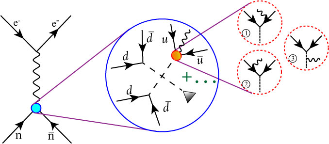
Figure 2: A neutron-antineutron transition is realized through electron-neutron scattering in a particular model of B-L violation. We consider the case in which the virtual photon interacts with the neutron through a six-fermion $|\Delta B|=2$ vertex generated through the spontaneous breaking of $(B-L)$-symmetry in the model of Ref. mohapatra1980local . A sample Feynman diagram is shown inside of the big blue circle, where the dashed line denotes a massive colored scalar. We represent the effective $q-\gamma-\bar{q}$ vertex by a red and gold circular area, which itself is realized by coupling the photon to any of the charged particles that appear. We explicitly show the diagrams that appear within three dashed red circles.

IV Matching from the quark to hadron level

Working in the quark basis, the effective Lagrangian that mediates $n-\bar{n}$ transitions without external sources is

$${\cal L}_{\rm n/q}\supset{\sum_{i,\chi_{1},\chi_{2},\chi_{3}}}^{\!\!\!\!\!\!\prime}(\delta_{i})_{\chi_{1},\chi_{2},\chi_{3}}({\cal O}_{i})_{\chi_{1},\chi_{2},\chi_{3}}+{\rm h.c.}\,,$$ (31)

where $i=1,2$, or $3$, and the prime denotes sums restricted to yield a non-redundant operator set, as per the discussion in Sec. III. We have already employed this form in determining the $n$-${\bar{n}}$ conversion operators. By analogy, the effective Lagrangian that mediates $n$-${\bar{n}}$ conversion is

$${\cal L}^{\rm conv}_{\rm n/q}\supset\sum_{\chi}{\sum_{i,\chi_{1},\chi_{2},\chi_{3}}}^{\!\!\!\!\!\!\prime}(\eta_{i})^{\chi}_{\chi_{1},\chi_{2},\chi_{3}}(\tilde{{\cal O}}_{i})^{\chi}_{\chi_{1},\chi_{2},\chi_{3}}+{\rm h.c.}\,,$$ (32)

though the precise nature of the restrictions in the sums requires further consideration. If the appearance of $n$-${\bar{n}}$ conversion derives from that of $n$-${\bar{n}}$ oscillation via electromagnetic interactions, then the $i,\chi_{1},\chi_{2},\chi_{3}$ sums are restricted as in Eq. (31). Moreover, the low-energy constants should not depend on $\chi$, and the surviving terms follow from computing the difference of $\chi=+$ and $\chi=-$. This in turn implies that only some of the possible $n$-${\bar{n}}$ oscillation operators contribute to $n$-${\bar{n}}$ conversion. It is precisely this prospect that makes experimental searches for $n$-${\bar{n}}$ oscillations and $n$-${\bar{n}}$ conversion genuinely complementary. However, once we have operators of form $(\tilde{{\cal O}}_{i})^{\chi}_{\chi_{1},\chi_{2},\chi_{3}}$, broader possibilities follow. If we are agnostic as to their origin, then the redundacies are those that follow from the flavor and color structure of the conversion operators themselves. Note that in this case we should also replace $Q_{u}/Q_{d}=-2$ in Eqs. (25) and (27) by $g_{\rm ratio}$, an unknown parameter. We find, e.g., that relations of the form of Eq. (10) exist:

$$(\tilde{\mathcal{O}}_{1})^{\chi}_{\chi_{1}LR}=(\tilde{\mathcal{O}}_{1})^{\chi}_{\chi_{1}RL}\,,\ \ (\tilde{\mathcal{O}}_{2,3})^{\chi}_{LR\chi_{3}}=(\tilde{\mathcal{O}}_{2,3})^{\chi}_{RL\chi_{3}}\,.$$ (33)

Moreover, in the case of $(\tilde{{\cal O}}_{1})^{\chi}_{\chi_{1},\chi_{2},\chi_{3}}$, the operator is also symmetric under $\chi\to-\chi$. Beginning with 48 possible operators, we find, finally, that there are $6$ independent operators of form $(\tilde{{\cal O}}_{1})^{\chi}_{\chi_{1},\chi_{2},\chi_{3}}$, and 12 independent operators of form $(\tilde{{\cal O}}_{i})^{\chi}_{\chi_{1},\chi_{2},\chi_{3}}$ for each $i=2,3$, though the $g_{\rm ratio}$ dependent terms should be separated into new operators if possible.

In what follows, we relate the low-energy constants that appear in this Lagrangian to those in the low-energy Lagrangian at the nucleon level, in which, due to the low energy scale, we regard the neutron and anti-neutron as point-like particles. In particular, noting Eq.(1), we relate the low-energy constants of this effective Lagrangian to those that appear at the quark level by equating the matrix elements of the pertinent operators. We have

$$\langle\bar{n}(\mathbf{p}^{\prime},s^{\prime})|\int d^{3}x{\cal L}_{\rm eff}^{({\rm conv})}|n(\mathbf{p},s)\rangle=\langle\bar{n}_{\rm q}(\mathbf{p}^{\prime},s^{\prime})|\int d^{3}x{\cal L}_{\rm n/q}^{({\rm conv})}|n_{\rm q}(\mathbf{p},s)\rangle\,,$$ (34)

where the states with the “q” subscripts are realized at the quark level. Explicitly, then,

$$\delta{\bar{v}}(\mathbf{p}^{\prime},s^{\prime})Cu(\mathbf{p},s)=\langle\bar{n}_{\rm q}(\mathbf{p}^{\prime},s^{\prime})|\int d^{3}x{\sum_{i,\chi_{1},\chi_{2},\chi_{3}}}^{\!\!\!\!\!\!\prime}(\delta_{i})_{\chi_{1},\chi_{2},\chi_{3}}({\cal O}_{i})_{\chi_{1},\chi_{2},\chi_{3}}|n_{\rm q}(\mathbf{p},s)\rangle\,$$ (35)

and

$$\eta{\bar{v}}(\mathbf{p}^{\prime},s^{\prime})C{\not{j}}\gamma_{5}u(\mathbf{p},s)=\langle\bar{n}_{\rm q}(\mathbf{p}^{\prime},s^{\prime})|\int d^{3}x\sum_{\chi}{\sum_{i,\chi_{1},\chi_{2},\chi_{3}}}^{\!\!\!\!\!\!\prime}(\eta_{i})^{\chi}_{\chi_{1},\chi_{2},\chi_{3}}(\tilde{{\cal O}}_{i})^{\chi}_{\chi_{1},\chi_{2},\chi_{3}}|n_{\rm q}(\mathbf{p},s)\rangle\,.$$ (36)

Using the connections we have derived in Eq. (26) and in and after Eq. (28) we can rewrite the latter as

$$\eta{\bar{v}}({\mathbf{p}}^{\prime},s^{\prime})C{\not{j}}\gamma_{5}u({\mathbf{p}},s)=\frac{em}{3(p_{\rm eff}^{2}-m^{2})}\frac{Qej_{\mu}}{q^{2}}\langle\bar{n}_{\rm q}(\mathbf{p}^{\prime},s^{\prime})|\!\!\int\!d^{3}x\!\!\!\!\!{\sum_{i,\chi_{1},\chi_{2},\chi_{3}}}^{\!\!\!\!\!\!\prime}\!(\delta_{i})_{\chi_{1},\chi_{2},\chi_{3}}[(\tilde{{\cal O}}_{i})^{{\rm R}\,\mu}_{\chi_{1},\chi_{2},\chi_{3}}\!-(\tilde{{\cal O}}_{i})^{{\rm L}\,\mu}_{\chi_{1},\chi_{2},\chi_{3}}]|n_{\rm q}(\mathbf{p},s)\rangle\,,$$ (37)

so that setting limits on $\eta$ can also constrain the quark-level low-energy constants associated with $n$-${\bar{n}}$ oscillations. We will determine that the operator matrix elements associated with $i=1$ vanish, so that $n$-${\bar{n}}$ conversion can only probe some of the $n$-${\bar{n}}$ oscillation operators. In the matching relations we have assumed that the quark-level low-energy constants are evaluated at the matching scale, subsuming evolution effects from the weak to QCD scales. Note, too, that we assume that “$\delta_{i}$” in Eqs. (35) and (37) are the same irrespective of such effects. Considering the matching relation of Eq. (37), we see that for a fixed experimental sensitivity to $\eta$ the limit on $(\delta_{i})_{\chi_{1}\chi_{2}\chi_{3}}$ will be sharpest if $q^{2}\simeq 0$. Thus in evaluating the hadron matrix elements we wish to choose $\mathbf{p}\simeq\mathbf{p}^{\prime}$. In the next section we compute the pertinent quark-level $n$-${\bar{n}}$ matrix elements explicitly using the M.I.T. bag model, for which the most convenient choice of kinematics is $\mathbf{p}=\mathbf{p}^{\prime}=0$.

V Matrix-element computations in the M.I.T. bag model

Table 1: Dimensionless matrix elements $(I_{i})^{\chi 3}_{\chi_{1}\chi_{2}\chi_{3}}$ of $n-\bar{n}$ conversion operators. The column “EM” denotes the matrix-element combination of $(\chi={\rm R})-(\chi={\rm L})$.

	$I_{1}$				$I_{2}$					$I_{3}$
$\chi_{1}\chi_{2}\chi_{3}$	$\chi=R$	$\chi=L$	EM	$\chi_{1}\chi_{2}\chi_{3}$	$\chi=R$	$\chi=L$	EM	$\chi_{1}\chi_{2}\chi_{3}$	$\chi=R$	$\chi=L$	EM
RRR	19.8	19.8	0	RRR	-4.95	-4.95	0	RRR	1.80	-8.28	10.1
RRL	17.3	17.3	0	RRL	-2.00	-9.02	7.02	RRL	-1.07	-8.81	7.74
RLR	17.3	17.3	0	RLR	-4.09	-0.586	-3.50	RLR	7.20	6.03	1.17
RLL	6.02	6.02	0	RLL	-0.586	-4.09	3.50	RLL	6.03	7.20	-1.17
LRR	6.02	6.02	0	LRR	-4.09	-0.586	-3.50	LRR	7.20	6.03	1.17
LRL	17.3	17.3	0	LRL	-0.586	-4.09	3.50	LRL	6.03	7.20	-1.17
LLR	17.3	17.3	0	LLR	-9.02	-2.00	-7.02	LLR	-8.78	-1.04	-7.74
LLL	19.8	19.8	0	LLL	-4.95	-4.95	0	LLL	-8.28	1.80	-10.1

Since the M.I.T. bag model is well known Chodos:1974pn ; Chodos:1974je , we only briefly summarize the ingredients that are important to our calculation. In this model, the quarks and antiquarks are confined in a static, spherical cavity of radius $R$ by a bag pressure $B$, within which they obey the free-particle Dirac equation. We only need the ground-state solutions, which we denote as $u^{s}_{\alpha,0}(\mathbf{r})$ ($v^{s}_{\alpha,0}(\mathbf{r})$) for a quark (antiquark) of flavor $\alpha$. We present their form and comment on the proper definition of $v^{s}_{\alpha,0}$ in Appendix B. The quantized quark field is given by

$$\psi^{i}_{\alpha}(\mathbf{r})=\sum_{n,s}[b^{i}_{\alpha s}(\mathbf{p}_{n})u^{s}_{\alpha,n}(\mathbf{r})+d^{i\dagger}_{\alpha s}(\mathbf{p}_{n})v^{s}_{\alpha,n}(\mathbf{r})]\,,$$ (38)

where $i$ is a color index and $b^{i}_{\alpha s}$ ($d^{i\dagger}_{\alpha s}$) denotes a quark (antiquark) annihilation (creation) operator, for which the non-null anticommutation relations are

$$\{b^{i}_{\alpha s}(\mathbf{p}),b^{j\dagger}_{\beta s^{\prime}}(\mathbf{p}^{\prime})\} = \delta_{ss^{\prime}}\delta_{ij}\delta_{\alpha\beta}\delta^{(3)}(\mathbf{p}-\mathbf{p}^{\prime}),$$ (39)

$$\{d^{i}_{\alpha s}(\mathbf{p}),d^{j\dagger}_{\beta s^{\prime}}(\mathbf{p}^{\prime})\} = \delta_{ss^{\prime}}\delta_{ij}\delta_{\alpha\beta}\delta^{(3)}(\mathbf{p}-\mathbf{p}^{\prime})\,.$$ (40)

The normalized neutron and antineutron wave functions are given by

$$|n\uparrow\rangle = (1/\sqrt{18})\epsilon^{ijk}(b^{i\dagger}_{u\uparrow}b^{j\dagger}_{d\downarrow}-b^{i\dagger}_{u\downarrow}b^{j\dagger}_{d\uparrow})b^{k\dagger}_{d\uparrow}|0\rangle,$$ (41)

$$|\bar{n}\uparrow\rangle = (1/\sqrt{18})\epsilon^{ijk}(d^{i\dagger}_{u\uparrow}d^{j\dagger}_{d\downarrow}-d^{i\dagger}_{u\downarrow}d^{j\dagger}_{d\uparrow})d^{k\dagger}_{d\uparrow}|0\rangle\,$$ (42)

where we use $|n\uparrow\rangle\equiv|n_{\rm q}(\mathbf{0},+)\rangle$ for spin up (and similarly for ${\bar{n}}$) and, following Rao and Shrock Rao:1982gt , we write the particular matrix elements of interest to us as

$$\langle\tilde{{\cal O}}_{i}\rangle^{\chi\,\mu}_{\chi_{1}\chi_{2}\chi_{3}} \equiv \langle\bar{n}\uparrow|\int d^{3}\mathbf{r}(\tilde{{\cal O}}_{i})^{\chi\,\mu}_{\chi_{1}\chi_{2}\chi_{3}}|n\uparrow\rangle=\left[\frac{N_{\alpha}^{6}}{(4\pi)^{2}p_{\alpha}^{3}}\right](I_{i})^{\chi\,\mu}_{\chi_{1}\chi_{2}\chi_{3}}\,.$$ (43)

We note that $(I_{i})^{\chi\,\mu}_{\chi_{1}\chi_{2}\chi_{3}}$ are dimensionless integrals, and we refer the reader to Appendix B for the form of the pre-factor and all other technical details. Picking the $z$ component for evaluation, we have

$$(I_{1})^{\chi 3}_{\chi_{1}\chi_{2}\chi_{3}} = -2\Big{(}B_{11}(\chi,\chi_{2},\chi_{3})+B_{11}(-\chi,\chi_{2},\chi_{3})\Big{)}+\Big{(}B_{12}(\chi_{1},\chi,\chi_{3})+B_{12}(\chi_{1},-\chi,\chi_{3})\Big{)}$$ (44)

$$+ \Big{(}B_{13}(\chi_{1},\chi_{2},\chi)+B_{13}(\chi_{1},\chi_{2},-\chi)\Big{)}\,;$$

$$(I_{j})^{\chi 3}_{\chi_{1}\chi_{2}\chi_{3}} = \Big{(}B_{j1}(\chi,\chi_{2},\chi_{3})-2B_{j1}(-\chi,\chi_{2},\chi_{3})\Big{)}+\Big{(}B_{j2}(\chi_{1},\chi,\chi_{3})-2B_{j2}(\chi_{1},-\chi,\chi_{3})\Big{)}$$ (45)

$$+ \Big{(}B_{j3}(\chi_{1},\chi_{2},\chi)+B_{j3}(\chi_{1},\chi_{2},-\chi)\Big{)}$$

for $j=2,3$, where

$$B_{11}(\chi_{1},\chi_{2},\chi_{3}) = -8i\Big{[}I_{a}-\frac{4}{3}\chi_{2}\chi_{3}I_{b}-8\chi_{2}\chi_{3}I_{c}\Big{]},$$ (46)

$$B_{12}(\chi_{1},\chi_{2},\chi_{3}) = -8i\Big{[}-2I_{a}-\frac{28}{3}\chi_{1}\chi_{3}I_{b}-8\chi_{1}\chi_{3}I_{c}\Big{]},$$ (47)

$$B_{13}(\chi_{1},\chi_{2},\chi_{3}) = -8i\Big{[}-2I_{a}-\frac{28}{3}\chi_{1}\chi_{2}I_{b}-8\chi_{1}\chi_{2}I_{c}\Big{]},$$ (48)

$$B_{21}(\chi_{1},\chi_{2},\chi_{3}) = -4i\Big{[}-\frac{1}{2}I_{a}+\frac{2}{3}\chi_{2}\chi_{3}I_{b}+4(\chi_{1}\chi_{3}-\chi_{1}\chi_{2})I_{b}+4\chi_{2}\chi_{3}I_{c}\Big{]},$$ (49)

$$B_{22}(\chi_{1},\chi_{2},\chi_{3}) = -4i\Big{[}-\frac{1}{2}I_{a}+\frac{2}{3}\chi_{1}\chi_{3}I_{b}+4(\chi_{2}\chi_{3}-\chi_{1}\chi_{2})I_{b}+4\chi_{1}\chi_{3}I_{c}\Big{]},$$ (50)

$$B_{23}(\chi_{1},\chi_{2},\chi_{3}) = -4i\Big{[}\frac{5}{2}I_{a}+\frac{26}{3}\chi_{1}\chi_{2}I_{b}+4\chi_{1}\chi_{2}I_{c}\Big{]},$$ (51)

and

$$B_{31}(\chi_{1},\chi_{2},\chi_{3}) = -\frac{1}{3}B_{21}(\chi_{1},\chi_{2},\chi_{3})-4i\Big{[}-\chi_{1}\chi_{2}I_{d}+4\chi_{2}\chi_{3}I_{e}\Big{]},$$ (52)

$$B_{32}(\chi_{1},\chi_{2},\chi_{3}) = -\frac{1}{3}B_{22}(\chi_{1},\chi_{2},\chi_{3})-4i\Big{[}-\chi_{1}\chi_{2}I_{d}+4\chi_{1}\chi_{3}I_{e}\Big{]},$$ (53)

$$B_{33}(\chi_{1},\chi_{2},\chi_{3}) = -\frac{1}{3}B_{23}(\chi_{1},\chi_{2},\chi_{3})-4i(3\chi_{1}\chi_{2}I_{f}),$$ (54)

with

$$I_{a}=\int^{\xi_{\alpha}}_{0}dx\,x^{2}[j^{2}_{0}(x)-\tilde{j}_{1}^{2}(x)]^{2}\Big{(}j^{2}_{0}(x)-\frac{1}{3}\tilde{j}^{2}_{1}(x)\Big{)}\,,\quad \!\!\!I_{b}=\int^{\xi_{\alpha}}_{0}dx\,x^{2}[j^{2}_{0}(x)-\tilde{j}_{1}^{2}(x)]j^{2}_{0}(x)\tilde{j}^{2}_{1}(x)\,,$$ (55)

$$I_{c}=\int^{\xi_{\alpha}}_{0}dx\,x^{2}j^{2}_{0}(x)\tilde{j}^{4}_{1}(x)\,,\quad \!\!\!I_{d}=\int^{\xi_{\alpha}}_{0}dx\,x^{2}[j^{2}_{0}(x)+\tilde{j}_{1}^{2}(x)][j^{2}_{0}(x)-\tilde{j}_{1}^{2}(x)]\Big{(}j^{2}_{0}(x)+\frac{1}{3}\tilde{j}^{2}_{1}(x)\Big{)}\,,$$ (56)

$$I_{e}=\int^{\xi_{\alpha}}_{0}dx\,x^{2}[j^{2}_{0}(x)+\tilde{j}_{1}^{2}(x)]j^{2}_{0}(x)\tilde{j}^{2}_{1}(x)\,,\quad \!\!\!I_{f}=\int^{\xi_{\alpha}}_{0}dx\,x^{2}[j^{2}_{0}(x)+\tilde{j}_{1}^{2}(x)]^{2}\Big{(}j^{2}_{0}(x)-\frac{1}{3}\tilde{j}^{2}_{1}(x)\Big{)}\,,$$ (57)

noting $\tilde{j}_{1}(x)\equiv\epsilon_{0}j_{1}(x)$. We have three input parameters, $m_{u}$, $m_{d}$, and $R$, which can be determined by fitting the hadron spectrum. For definiteness we use the same fits as employed by Rao and Shrock Rao:1982gt , in which $m_{u}=m_{d}$. Picking the fit with nonzero quark mass, so that $m_{u}=m_{d}=0.108\,{\rm GeV}$ and $R=5.59\,{\rm GeV}^{-1}$, we evaluate $N_{\alpha}^{6}/(4\pi)^{2}p_{\alpha}^{3}=0.529\times 10^{-5}\,{\rm GeV}^{6}$ (noting $\xi_{\alpha}\simeq 2.281$), as well as $I_{a}=0.298$, $I_{b}=0.0344$, $I_{c}=0.0106$, $I_{d}=0.396$, $I_{e}=0.0557$, and $I_{f}=0.460$. Dropping the common factor of $i$, we evaluate $(I_{i})^{\chi 3}_{\chi_{1}\chi_{2}\chi_{3}}$ numerically and report the results in Table 1. As a numerical check, we have also computed the matrix elements of the $n-{\bar{n}}$ oscillation operators $({\cal O}_{i})_{\chi_{1}\chi_{2}\chi_{3}}$, and we reproduce Rao and Shrock’s results up to an overall factor of $-i$ Rao:1982gt . The pattern of these results, i.e., the sign and relative sizes, agree with recent lattice QCD results Syritsyn:2016ijx , though the latter are of larger absolute size. We note that the results of Table 1 bear out the symmetries of Eq. (33) and the $\chi\to-\chi$ symmetry of $(\tilde{{\cal O}}_{1})^{\chi}_{\chi_{1},\chi_{2},\chi_{3}}$. Consequently, upon making the matrix element combination $(\chi={\rm R})-(\chi={\rm L})$, as would occur if the conversion operators appear only via electromagnetic interactions, the contributions from $(\tilde{{\cal O}}_{1})^{\chi}_{\chi_{1},\chi_{2},\chi_{3}}$ vanish as expected. This underscores the complementarity of $n$-${\bar{n}}$ conversion and oscillation searches. Note, moreover, if we were to restrict our consideration to the conversion operators that stem from electromagnetism and SU(2)${}_{L}\times$U(1)_Y invariant $n$-${\bar{n}}$ oscillation operators, only the terms from $({\cal O}_{3})_{LRR}$ and $({\cal O}_{3})_{LLR}$ would survive.

VI Numerical Estimates and Experimental Prospects

We now turn to the numerical evaluation of the matching relations in Eqs. (35,36,37). In the kinematic limit for which $\mathbf{p}=\mathbf{p}^{\prime}=0$, the left-hand sides of Eq. (35) and Eqs. (36,37) become $\delta\delta_{s,s^{\prime}}$ and $\eta(j^{z}s\delta_{s,s^{\prime}}+j^{x}\delta_{s,-s^{\prime}}+isj^{y}\delta_{s,-s^{\prime}})$, respectively. As a numerical check, we have verified that our numerical matching procedure does not depend on the particular non-zero component we pick. Generally, a plurality of quark-level operators can contribute to either $n$-${\bar{n}}$ oscillation or conversion; however, if a single operator dominates each case, then the experimental limits from the two processes can potentially be compared directly. Choosing $\mu=z$ as in the last section and supposing for illustration that only $({\cal{O}}_{3})_{LLR}$ operates through electromagnetism, we find

$$(\delta_{3})_{LLR}\left((I_{3})^{R3}_{LLR}-(I_{3})^{L3}_{LLR}\right)\frac{e}{3}\frac{m}{p_{\rm eff}^{2}-m^{2}}\frac{Qej_{z}}{q^{2}}=\eta j_{z}\,,$$ (58)

whereas $(\delta_{3})_{LLR}\langle\mathcal{O}_{3}\rangle_{LLR}=\delta$. Combining these relations we can thus relate a would-be limit on $\eta$ to one on $\delta$, namely

$$\eta=\frac{\delta}{q^{2}}\frac{Qe^{2}}{3}\left(\frac{m}{p_{\rm eff}^{2}-m^{2}}\right)\frac{\left((I_{3})^{R3}_{LLR}-(I_{3})^{L3}_{LLR}\right)}{\langle\mathcal{O}_{3}\rangle_{LLR}}\,,$$ (59)

so that with $\eta\equiv\beta\delta Qe^{2}/q^{2}$ we have

$$\beta\equiv\frac{1}{3}\left(\frac{m}{p_{\rm eff}^{2}-m^{2}}\right)\frac{\left((I_{3})^{R3}_{LLR}-(I_{3})^{L3}_{LLR}\right)}{\langle\mathcal{O}_{3}\rangle_{LLR}}=\frac{1}{3}\left(\frac{0.108}{(0.365)^{2}}\right)\frac{(-7.72)}{2.03}\ \text{GeV}^{-1}\simeq-0.946\ \text{GeV}^{-1}\,.$$ (60)

In evaluating the kinematic factors we replace $p_{\rm eff}^{2}-m^{2}$ with $E_{\alpha}^{2}-m^{2}=p_{\alpha}^{2}$ as an estimate of a quark’s off-shellness. Noting Table 1, we see that other operators can also be used as distinct choices, with the associated values of $\beta$ ranging to roughly ten times smaller or larger. Returning to Eq. (37) we see we can recast the connection to the $n$-${\bar{n}}$ oscillation parameters more generally by replacing $\delta$ with $\tilde{\delta}$, where

$$\tilde{\delta}\equiv\left[\frac{\langle\mathcal{O}_{3}\rangle_{LLR}}{(I_{3})^{R3}_{LLR}-(I_{3})^{L3}_{LLR}}\right]\!\!{\sum_{\chi_{1},\chi_{2},\chi_{3}}}^{\!\!\!\!\!\!\prime}\!\!\left[(\delta_{2})_{\chi_{1},\chi_{2},\chi_{3}}\!\left((I_{2})^{{\rm R}\,3}_{\chi_{1},\chi_{2},\chi_{3}}\!\!\!-(I_{2})^{{\rm L}\,3}_{\chi_{1},\chi_{2},\chi_{3}}\right)+(\delta_{3})_{\chi_{1},\chi_{2},\chi_{3}}\!\left((I_{3})^{{\rm R}\,3}_{\chi_{1},\chi_{2},\chi_{3}}\!\!\!-(I_{3})^{{\rm L}\,3}_{\chi_{1},\chi_{2},\chi_{3}}\right)\right]$$ (61)

where we neglect any momentum dependence in the nucleon matrix element.

To study the possible limits on $\eta$ and hence $\tilde{\delta}$, we consider the process $n(p_{n})+\ell(p_{\ell})\rightarrow\bar{n}(p_{n}^{\prime})+\ell(p_{\ell}^{\prime})$, where $\ell$ is a charged lepton, or, more generally, any electrically charged particle. We study the limits on $\eta$ that would arise if we were to neglect the connection to $n$-${\bar{n}}$ oscillations in a separate paper svgxy_search17 . To make numerical estimates of the sensitivity to $\tilde{\delta}$, we consider different possible combinations of beam and target — and different energy regimes as well, though we restrict our considerations to center-of-mass energies well below nucleon-antinucleon production threshold. In all cases, however, the best limits on $\tilde{\delta}$ emerge if we consider kinematics in which the squared momentum transfer $q^{2}$ is minimized.

To evaluate the scattering process, we note that the lowest-order amplitude in our effective field theory is simply $i\mathcal{M}=\eta\bar{u}_{\ell}(p^{\prime}_{\ell})(\gamma^{\mu})u_{\ell}(p_{\ell})v^{T}_{n}(p^{\prime}_{n})C\gamma_{\mu}\gamma^{5}u_{n}(p_{n})$, so that the spin-averaged, absolute-squared amplitude $\overline{|\mathcal{M}|^{2}}$ is

$$\overline{|\mathcal{M}|^{2}}=\frac{8Q_{\ell}^{2}e^{4}|\beta|^{2}\tilde{\delta}^{2}}{q^{4}}\Big{[}(p^{\prime}_{\ell}\cdot p^{\prime}_{n})(p_{\ell}\cdot p_{n})+(p^{\prime}_{n}\cdot p_{\ell})(p^{\prime}_{\ell}\cdot p_{n})-2m_{\ell}^{2}M^{2}+M^{2}(p^{\prime}_{\ell}\cdot p_{\ell})-m_{\ell}^{2}(p^{\prime}_{n}\cdot p_{n})\Big{]},$$ (62)

where we introduce $q^{2}\equiv(p_{\ell}-p^{\prime}_{\ell})^{2}$ and $\overline{|{\mathcal{M}}^{\prime}|^{2}}$ for the quantity in square brackets for subsequent use. The differential cross section is

$$d\sigma=\frac{1}{F}\frac{d^{3}p^{\prime}_{\ell}}{(2\pi)^{3}}\frac{1}{2E^{\prime}_{\ell}}\frac{d^{3}p^{\prime}_{n}}{(2\pi)^{3}}\frac{1}{2E^{\prime}_{n}}\overline{|\mathcal{M}|^{2}}(2\pi)^{4}\delta^{4}(p_{\ell}+p_{n}-p^{\prime}_{\ell}-p^{\prime}_{n}),$$ (63)

where the flux factor $F$ is $4((p_{n}\cdot p_{\ell})^{2}-m_{\ell}^{2}M^{2})^{1/2}$. In what follows we evaluate the cross sections for electron-neutron scattering in various kinematics. We employ beam parameters and target densities as established at existing experiments and facilties, or their planned extensions, to estimate the limits on $\tilde{\delta}$ that can emerge through $n$-${\bar{n}}$ conversion.

We begin with the case of an electron beam scattering from a neutron bound in a deuterium target, e.g., because a free neutron target is unavailable. In such a scenario the converted ${\bar{n}}$ is left in situ, to annihilate with the material around it. In the alternate case of a neutron beam scattering from an atomic target, the converted ${\bar{n}}$ emerges with roughly the same momentum as the incoming beam, so that the location of the annihilation products serves as a background discriminant. In nuclear stability studies, experimental backgrounds arise from the interactions of atmospheric neutrinos within the experimental volume, producing charged leptons and hadrons, and they have been studied in detail, noting Refs. Abe:2011ky ; Aharmim:2017jna , e.g. Neutrinos could also potentially mediate the reaction ${\bar{\nu}}{n}\to\bar{n}\nu$, which would seem to suggest that a $n\to{\bar{n}}$ process could appear without breaking B-L symmetry. However, this effect should be negligibly small because it contains the product of a $|\Delta B|=2$ and a $|\Delta L|=2$ transition. In contrast to nuclear stability studies, it has proved possible to conduct a sensitive experimental search for free $n$-${\bar{n}}$ oscillation such that no background events that would mimic the signal appear baldo1994new .

VI.1 Electron scattering from a deuterium target

We evaluate the cross section for electron-neutron scattering, neglecting the effect of nuclear binding. Integrating over phase space using Eqs. (62) and (63), assuming the neutron is initially at rest, we have

$$\frac{d\sigma}{d\Omega} = \frac{e^{4}|\beta|^{2}{\tilde{\delta}}^{2}}{8\pi^{2}M|\boldsymbol{p}_{e}|}\left(\frac{|\boldsymbol{p^{\prime}}_{e}|^{2}}{|\boldsymbol{p^{\prime}}_{e}|(M+E_{e})-|\boldsymbol{p}_{e}|E^{\prime}_{e}\cos\theta}\right)\frac{\overline{|{\mathcal{M}}^{\prime}|^{2}}}{q^{4}}\Big{|}_{p^{\prime}_{n}=p_{e}+p_{n}-p^{\prime}_{e}\,;\,E_{e}^{\prime}=\chi_{e}}\,,$$ (64)

where $\theta$ is the angle between $\boldsymbol{p^{\prime}}_{e}$ and $\boldsymbol{p}_{e}$ and $E_{e}^{\prime}=\chi_{e}$ is the solution to

$$2M(E_{e}-E_{e}^{\prime})+2m_{e}^{2}-2E_{e}E_{e}^{\prime}+2|\boldsymbol{p}_{e}|\sqrt{E_{e}^{\prime 2}-m_{e}^{2}}\cos\theta=0\,.$$ (65)

The cross section grows as $\theta^{-4}$ as $\theta$ approaches zero, so that we can assess its size for fixed $\tilde{\delta}$ by first estimating the minimum value of $\theta_{0}$. Noting Ref. Fernow:1986 , we determine $\theta_{0}$ in two different ways and then choose the larger value for our cross section estimate. (i) Using the Coulomb interaction between the incoming charged particle and the charged particles of the deuterium target, we estimate

$$\theta_{0}\approx\frac{2\alpha}{r_{a}|\boldsymbol{p_{e}}|}=\frac{2m_{e}\alpha^{2}}{|\boldsymbol{p_{e}}|}=5.45\times 10^{-7}\,\hbox{rad}\,,$$ (66)

where we use $|\boldsymbol{p_{e}}|=100\,{\hbox{MeV}}$. (ii) Alternatively, by the uncertainty principle, hitting an atom of $r_{a}$ in transverse size implies the incident momentum is smeared by $1/r_{a}$, so that the associated minimum scattering angle is

$$\theta_{0}\approx\frac{1}{|\boldsymbol{p}_{e}|r_{a}}=\frac{m_{e}\alpha}{|\boldsymbol{p}_{e}|}=3.73\times 10^{-5}\,\hbox{rad}\,,$$ (67)

where the radius of the hydrogen atom is used for $r_{a}$. Thus we see that the two angular estimates are not the same, and we proceed to estimate the total cross section as per

$$\sigma\approx\frac{d\sigma}{d\Omega}\Big{|}_{\theta=\theta_{0}}\times\pi\theta_{0}^{2}\,,$$ (68)

and the larger $\theta_{0}$, so that our total cross section estimate is

$$\sigma\approx\left[|\tilde{\delta}|^{2}\ 5.12\times 10^{7}\right]\ \text{GeV}^{-2}\,,$$ (69)

where $|\tilde{\delta}|$ is understood to be in units of GeV. We note that as long as $\boldsymbol{p}_{e}\gg m_{e}$ and $\theta_{0}\propto 1/|\boldsymbol{p}_{e}|$, the estimate no longer depends on $|\boldsymbol{p}_{e}|$. To determine the sensitivity to $\tilde{\delta}$, we must compute the event rate $dN/dt$ and finally the expected yield of events. We have

$$\frac{dN}{dt}={\cal L}\sigma=\phi\rho_{T}L\sigma\,,$$ (70)

where the luminosity ${\cal L}$ is in units of particles/s-cm², $\phi$ is the flux in units of particles/s, $\rho_{T}$ is the target number density, and $L$ is its length. We turn to the DarkLight experiment operating at the Free-Electron Laser (FEL) facility of Jefferson National Accelerator Laboratory (JLab) for suitable electron beam parameters Corliss:2017tms ; Alarcon:2013bca ; Neil:2005jy . The beam energy that experiment employs is $100$ MeV, and its current is 10 mA, for a beam power of 1 MW; it also uses a gaseous hydrogen target. In our case we would favor a liquid deuterium target, however, because it is denser, noting, e.g., its use in the experiment of Ref. Ito:2003mr , but target heating may preclude its use under DarkLight conditions. To consider this issue further we turn to the Qweak experiment at JLab Allison:2014tpu , which uses a liquid hydrogen target and an electron beam with energy $E=1.16\ \text{GeV}$ and a beam current of $180\ \mu A$, yielding a beam power in this latter case of $0.209$ MW. Thus for the estimate in our case, we suppose that we can lower the beam energy to 20 MeV, but keep the same beam current, so that the beam power will be within the range of the Qweak experiment and a liquid deuterium target can be used. The electron beam flux in this case is $0.6\times 10^{17}\,\text{s}^{-1}$, the number density of liquid deuterium is $\rho_{d}=5.1\times 10^{22}\ \text{cm}^{-3}$ at 19 K clusius , and if we suppose a 1 m long target and a running time of 1 year, the sensitivity to $\tilde{\delta}$ for $N$ signal events is

$$|\tilde{\delta}|\lesssim 2\times 10^{-15}\sqrt{\frac{N\ \text{events}}{1\ \text{event}}}\sqrt{\frac{1\ \text{yr}}{\text{t}}}\sqrt{\frac{0.6\times 10^{17}\ \text{s}^{-1}}{\phi}}\sqrt{\frac{1\ \text{m}}{L}}\sqrt{\frac{5.1\times 10^{22}\ \text{cm}^{-3}}{\rho}}\ \text{GeV}.$$ (71)

VI.2 Neutron scattering from atomic targets

We now turn to the evaluation of neutron scattering from the charged particles of an atomic target. In this case the scattering cross section is dominated by the electron contribution, and we can ignore the role of electromagnetic $n-p$ scattering completely. However, it is important to pick a target for which the loss of neutrons from neutron capture would be minimal. In this regard, a deuterium target would be a good choice because the measured thermal neutron capture cross section on deuterium is merely $\sigma_{\rm c}=0.508\pm 0.015\ \text{mb}$ Jurney:1982zz , so that neutron capture effects would have a very limited impact on the transmitted flux. That is, noting that the neutron flux loss would be controlled by $\phi=\phi_{0}\exp(-\sigma_{c}L\rho_{d})$, we have $\phi/\phi_{0}\simeq 0.998$ if $L=1\ \text{m}$. Although the capture cross section scales inversely with the neutron velocity at low energies, capture effects are also negligible for cold neutron energies, noting a kinetic energy of $T_{n}\approx 10^{-3}\ \text{eV}$ for reference. Thus we regard a deuterium target as a suitable choice, though there are others, notably one of ¹⁶O. Potentially one could also consider neutron scattering from an electron plasma, confined by a magnetic field, but in this case the electron density is limited brillouin — and much greater electon number densities can easily be found in atomic targets. Thus we focus on the use of deuterium and oxygen targets.

To determine the differential cross section for neutron-electon scattering, we need only switch the roles of the neutron and electron in the evaluation of the phase space integrals in Eq. (64). Certainly the differential cross section is still largest in the forward direction, and we continue to use Eq. (68) to estimate the total cross section. Solving the analog of Eq. (65) for $E_{n}^{\prime}$ reveals that the neutron scattering angle is restricted, that is, $m_{e}^{2}-M^{2}\sin^{2}\theta\geq 0$ is a necessary consequence of the kinematics. We use the largest allowed scattering angle in our $n-e$ cross section estimate, yielding $\theta_{\rm max}\leq m_{e}/M\approx 5.44\times 10^{-4}\,\text{rad}$. In the case of $n-p$ scattering, the scattering angle is no longer restricted, and the most reasonable choice of angle depends on the momentum of the neutron beam. For neutrons with a kinetic energy of 100 MeV, e.g., we find $|\boldsymbol{p}_{n}|=\sqrt{2MT_{n}}\approx 447\,\text{MeV}$, and in this case we adapt our uncertainty principle estimate of Eq. (67) to write $\theta_{\rm min}\approx 1/|\boldsymbol{p}_{n}|r_{a}$ and use that angle in our estimate. For cold neutrons, noting the conditions of the experiment of Ref. baldo1994new , we consider a kinetic energy of $T_{n}=2\times 10^{-3}\ \text{eV}$, which corresponds to an average neutron wavelength $\lambda\approx 6.5$ Å and $|\boldsymbol{p}_{n}|\approx 1.94\ \text{keV}$. In this case, the uncertainty principle does not provide a useful restriction on the angle, but low-energy, forward-scattering experiments with neutrons are certainly possible nonetheless. The authors of Ref. Bowman:2014fca note that it should be possible to detect a scattering angle of $0.003\ \text{rad}$, and for definiteness we employ this angle for our low-energy $n-p$ cross section estimate. Herewith we summarize our $n-e$ and $n-p$ cross section results. For $|\boldsymbol{p}_{n}|=0.447\ \text{GeV}$ we have

$$\sigma_{n-e}=\left[|\tilde{\delta}|^{2}\ 5.74\times 10^{7}\right]\ \text{GeV}^{-2}\quad;\quad\sigma_{n-p}=\left[|\tilde{\delta}|^{2}\ 3.96\times 10^{2}\right]\ \text{GeV}^{-2}\,,$$ (72)

whereas for $|\boldsymbol{p}_{n}|=1.94\ \text{keV}$ we have

$$\sigma_{n-e}=\left[|\tilde{\delta}|^{2}0.881\times 10^{21}\right]\ \text{GeV}^{-2}\quad;\quad\sigma_{n-p}=\left[|\tilde{\delta}|^{2}\ 1.98\times 10^{13}\right]\ \text{GeV}^{-2}\,.$$ (73)

The $n-e$ and low-energy $n-p$ results should be regarded as lower bounds. Nevertheless, it is apparent that the effects of $n-p$ interactions are relatively negligible, and we ignore them in our sensitivity estimates to follow. For the cold neutron case, we employ the beam parameters of the ILL experiment baldo1994new , so that we use $\phi\simeq 1.7\times 10^{11}\ \text{s}^{-1}$ in our estimate. For the higher energy case, we note the study of high-energy (1-120 MeV) neutron flux spectra at the Spallation Neutron Source (SNS) in Fig. 5.12 of Ref. luciano , so that we employ a flux of $\phi=5\times 10^{8}\ \text{s}^{-1}$ in that case. Thus for $|\boldsymbol{p_{n}}|=0.447\ \text{GeV}$ the sensitivity to $|\tilde{\delta}|$ is

$$|\tilde{\delta}|\lesssim 2\times 10^{-11}\sqrt{\frac{N\ \text{events}}{1\ \text{event}}}\sqrt{\frac{1\ \text{yr}}{\text{t}}}\sqrt{\frac{5\times 10^{8}\ \text{s}^{-1}}{\phi}}\sqrt{\frac{1\ \text{m}}{L}}\sqrt{\frac{5\times 10^{22}\ \text{cm}^{-3}}{\rho}}\ \text{GeV}\,,$$ (74)

whereas for $|\boldsymbol{p_{n}}|=1.94\ \text{keV}$, we have

$$|\tilde{\delta}|\lesssim 3\times 10^{-19}\sqrt{\frac{N\ \text{events}}{1\ \text{event}}}\sqrt{\frac{1\ \text{yr}}{\text{t}}}\sqrt{\frac{1.7\times 10^{11}\ \text{s}^{-1}}{\phi}}\sqrt{\frac{1\ \text{m}}{L}}\sqrt{\frac{5\times 10^{22}\ \text{cm}^{-3}}{\rho}}\ \text{GeV}\,.$$ (75)

Finally, we turn to the case of a solid ¹⁶O target, for which the at 24 K is $\rho_{o}=5.76\times 10^{22}\text{cm}^{-3}$ roder . Here, too, we focus on the $n-e$ scattering contribution. Since each O atom has eight electrons, the cross section should be eight times larger. Thus for $|\boldsymbol{p_{n}}|=0.447\ \text{GeV}$ we estimate a sensitivity of

$$|\tilde{\delta}|\lesssim 7\times 10^{-12}\sqrt{\frac{N\ \text{events}}{1\ \text{event}}}\sqrt{\frac{1\ \text{yr}}{\text{t}}}\sqrt{\frac{5\times 10^{8}\ \text{s}^{-1}}{\phi}}\sqrt{\frac{1\ \text{m}}{L}}\sqrt{\frac{5.76\times 10^{22}\ \text{cm}^{-3}}{\rho}}\ \text{GeV}\,,$$ (76)

whereas for $|\boldsymbol{p_{n}}|=1.947\ \text{keV}$ we have

$$|\tilde{\delta}|\lesssim 1\times 10^{-19}\sqrt{\frac{N\ \text{events}}{1\ \text{event}}}\sqrt{\frac{1\ \text{yr}}{\text{t}}}\sqrt{\frac{1.7\times 10^{11}\ \text{s}^{-1}}{\phi}}\sqrt{\frac{1\ \text{m}}{L}}\sqrt{\frac{5.76\times 10^{22}\ \text{cm}^{-3}}{\rho}}\ \text{GeV}\,.$$ (77)

It appears that the greatest sensitivity to the $n$-${\bar{n}}$ oscillation parameter $\tilde{\delta}$ can be realized through cold neutron beams scattering from atomic (or molecular) deuterium or ¹⁶O targets. We wish to emphasize that these particular estimates rely on choosing the largest value of a very small scattering angle, supposing that the detection of annihilation events would rely on their displacement away from the forward direction. We note that the measurement of much smaller momentum transfers in neutron scattering than we have considered are under development vsans , and the realization of this could ultimately lead to significant improvements in sensitivity. Improvements could also come from the use of brighter neutron beams. This could be realizable, e.g., with the planned LD₂ cold source for the NG-C guide at NIST, where we refer to Fig. 8 in Ref. Cook:2009 for further details. The best prospects in this regard, however, should be offered by the European Spallation Source (ESS), noting Refs. phillips2016neutron ; milstead2015new for a description of the possibilities.

VII Summary and Outlook

In this paper we have considered the process of $n$-${\bar{n}}$ conversion, in which a $|\Delta B|=2$ transition, which breaks B-L symmetry, is mediated by an external source. The observation of such a process would reveal the existence of physics beyond the SM and indeed that of fundamental Majorana dynamics. In contradistinction to $n$-${\bar{n}}$ oscillation, in which a neutron spontaneously converts into an antineutron, the process is not sensitive to the presence of fields and matter in the external environment because energy-momentum conservation is ensured through the participation of an external current. We have developed the connections between $n$-${\bar{n}}$ conversion and $n$-${\bar{n}}$ oscillation, noting, in particular, that operators that give rise to spontaneous $n$-${\bar{n}}$ transitions can also give rise to $n$-${\bar{n}}$ conversion via an external electromagnetic current, because the quarks carry electric charge. We have determined precisely how quark-level conversion operators can be determined in this case and, moreover, how only certain of the operators that generate $n$-${\bar{n}}$ oscillation can also generate $n$-${\bar{n}}$ conversion. Thus searches for $n$-${\bar{n}}$ conversion are genuinely complementary to those for $n$-${\bar{n}}$ oscillation.

We have also studied the inferred limits on the subset of low-energy constants associated with $n$-${\bar{n}}$ oscillation that could arise from $n$-${\bar{n}}$ conversion searches. We have found that the connection is sharpest when the momentum transfer associated with the scattering is smallest, so that the higher-mass-dimension conversion operator is the least suppressed. We have, moreover, evaluated a number of electron-neutron scattering processes and have found that cold neutron beams scattering from atomic (or molecular) deuterium or oxygen targets appear to have the greatest sensitivity. Generally our anticipated limits are much less severe than those associated with direct searches for $n$-${\bar{n}}$ oscillation, recalling that the free neutron limit from the ILL experiment can be expressed as $\delta\leq 5\times 10^{-32}\,\hbox{GeV}$ at 90% CL baldo1994new , but the set of probed operators is different. Also a quantitative understanding of the manner in which the spontaneous process is suppressed by external fields and matter is necessary to assessing those limits. The study of B-L violation in scattering does not have such a liability, and we note the prospects for the discovery of B-L violation via $n$-${\bar{n}}$ conversion without reference to $n$-${\bar{n}}$ oscillation in a separate paper svgxy_search17 .

Finally we would like to note that the mechanism of $n$-${\bar{n}}$ conversion can lead to broader studies of the spin and flavor dependence of B-L violating processes. We note the prospect of $\Delta^{0}-\bar{\Delta}^{0}$ transitions, as well as that of $n-\bar{\Delta}^{0}$, although the quark-level operators that appear are shared by $n$-${\bar{n}}$ conversion. It is also possible to probe B-L violating operators that also change strangeness, mediating, e.g., $n-\bar{\Lambda}$ and $n-\bar{\Sigma}^{0}$ transitions basecq1983deltab , or $\Lambda_{0}-{\bar{\Lambda}}_{0}$ transitions Kang:2009xt ; Addazi:2017iho . More generally, we note that the ongoing technical efforts in the realization of the next generation of high-intensity electron and neutron beams can have an immediate impact on fundamental physics through searches for B-L violation via $n$-${\bar{n}}$ conversion.

Appendices

A Definitions and conventions

In this appendix we collect the definitions and basic results that underlie the central arguments of the paper. The discrete-symmetry transformations of a four-component fermion field $\psi(x)$ are given by

$$\mathbf{C}\psi(x)\mathbf{C}^{-1}=\eta_{c}C\gamma^{0}\psi^{\ast}(x)\equiv\eta_{c}i\gamma^{2}\psi^{\ast}(x)\equiv\eta_{c}\psi^{c}(x)\,,$$ (78)

$$\mathbf{P}\psi(t,\mathbf{x})\mathbf{P}^{-1}=\eta_{p}\gamma^{0}\psi(t,-\mathbf{x})\,,$$ (79)

$$\mathbf{T}\psi(t,\mathbf{x})\mathbf{T}^{-1}=\eta_{t}\gamma^{1}\gamma^{3}\psi(-t,\mathbf{x})\,,$$ (80)

where $\eta_{c}$, $\eta_{p}$, and $\eta_{t}$ are unimodular phase factors of the charge-conjugation C, parity P, and time-reversal T transformations, respectively, and we have chosen the Dirac-Pauli representation for the gamma matrices. Furthermore the unimodular factors are constrained so that $\eta_{c}\eta_{p}\eta_{t}$ and $\eta_{p}$ are pure imaginary gardner2016c .

The plane-wave expansion of a Dirac field $\psi(x)$ (noting $\hbar=c=1$) is given by

$$\psi(x)=\int\frac{d^{3}\mathbf{p}}{(2\pi)^{3/2}\sqrt{2E}}\sum_{s=\pm}\left\{b(\mathbf{p},s)u(\mathbf{p},s)e^{-ip\cdot x}+d^{\dagger}(\mathbf{p},s)v(\mathbf{p},s)e^{ip\cdot x}\right\}\,,$$ (81)

with spinors defined as

$$u(\mathbf{p},s)={\cal N}\left(\begin{array}[]{c}\chi^{(s)}\\ \frac{\mathbf{\sigma}\cdot\mathbf{p}}{E_{p}+M}\chi^{(s)}\\ \end{array}\right)\quad;\quad v(\mathbf{p},s)={\cal N}\left(\begin{array}[]{c}\frac{\mathbf{\sigma}\cdot\mathbf{p}}{E_{p}+M}\chi^{\prime\,(s)}\\ \chi^{\prime(s)}\\ \end{array}\right)\,,$$ (82)

noting $\chi^{\prime\,(s)}=-i\sigma^{2}\chi^{(s)}$, $\chi^{+}=\left(\stackrel{{\scriptstyle 1}}{{{}_{0}}}\right)$, $\chi^{-}=\left(\stackrel{{\scriptstyle 0}}{{{}_{1}}}\right)$, and ${\cal N}=\sqrt{E_{p}+M}$. The pertinent fermion anticommutation relations are $\{b(\mathbf{p},s),b^{\dagger}(\mathbf{p^{\prime}},s^{\prime})\}=\{d(\mathbf{p},s),d^{\dagger}(\mathbf{p^{\prime}},s^{\prime})\}=\delta^{(3)}(\mathbf{p}-\mathbf{p^{\prime}})\delta^{s\,s^{\prime}}$; all others vanish. We also give the single-particle states a covariant normalization; e.g.,

$$|n(\mathbf{p},s)\rangle=\sqrt{2E_{p}}(2\pi)^{3/2}b^{\dagger}(\mathbf{p},s)|0\rangle\,.$$ (83)

With these choices we recover the usual form of the equal-time commutation relations in $\psi(x)$ and $\bar{\psi}(x)$ and that of $\langle n(\mathbf{p},s)|n(\mathbf{p^{\prime}},s^{\prime})\rangle$ Peskin:1995ev .

We also note the convenient relationships

$$v^{T}(\mathbf{p},s)C={\bar{u}}(\mathbf{p},s)\quad;\quad u^{T}(\mathbf{p},s)C={\bar{v}}(\mathbf{p},s)\;,$$ (84)

as well as

$$\bar{u}(\mathbf{p},s)\gamma^{\mu}u(\mathbf{p}^{\prime},s^{\prime}) = \bar{v}(\mathbf{p}^{\prime},s^{\prime})\gamma^{\mu}v(\mathbf{p},s)\,,$$ (85)

$$\bar{u}(\mathbf{p},s)\gamma^{\mu}\gamma_{5}u(\mathbf{p}^{\prime},s^{\prime}) = -\bar{v}(\mathbf{p}^{\prime},s^{\prime})\gamma^{\mu}\gamma_{5}v(\mathbf{p},s)\,,$$ (86)

where the latter follow from computing the transpose of the left-hand side in each case.

B The ground-state antiparticle in the M.I.T. bag model

In the M.I.T. bag model, the quarks and antiquarks obey the free-particle Dirac equation within a spherical cavity of radius $R$, subject to boundary conditions at its surface Chodos:1974pn ; Chodos:1974je . Solutions of opposite parity, i.e., with $k=\mp 1$ exist:

$$\psi_{\alpha(k=-1)}(\mathbf{r}) = \frac{N_{\alpha}}{\sqrt{4\pi}}\begin{pmatrix}ij_{0}(p_{\alpha}\mathbf{r})\chi^{(s)}\\ -\epsilon_{\alpha}j_{1}(p_{\alpha}\mathbf{r})\mathbf{\sigma}\cdot\hat{\mathbf{r}}\chi^{(s)}\end{pmatrix},$$ (87)

$$\psi_{\alpha(k=1)}(\mathbf{r}) = \frac{{\tilde{N}}_{\alpha}}{\sqrt{4\pi}}\begin{pmatrix}ij_{1}(p_{\alpha}\mathbf{r})\mathbf{\sigma}\cdot\hat{\mathbf{r}}\chi^{(s)}\\ \epsilon_{\alpha}j_{0}(p_{\alpha}\mathbf{r})\chi^{(s)}\end{pmatrix},$$ (88)

where

$$N_{\alpha} = \Big{(}\frac{\xi_{\alpha}^{2}j^{-2}_{0}(\xi_{\alpha})}{R^{3}[2E_{\alpha}R(E_{\alpha}R-1)+mR]}\Big{)}^{\frac{1}{2}},$$ (89)

$${\tilde{N}}_{\alpha} = \Big{(}\frac{\xi_{\alpha}^{2}j^{-2}_{1}(\xi_{\alpha})}{R^{3}[2E_{\alpha}R(E_{\alpha}R+1)+mR]}\Big{)}^{\frac{1}{2}}\,,$$ (90)

and $j_{n}$ is a spherical Bessel function of the first kind of order $n$, with $m$ and $s$ denoting the quark mass and spin, respectively. Also

$$p_{\alpha}=\frac{\xi_{\alpha}}{R}\,,\quad E^{2}_{\alpha}=p^{2}_{\alpha}+m^{2}\,,\quad\epsilon_{\alpha}=\sqrt{\frac{E_{\alpha}-m}{E_{\alpha}+m}}\,,$$ (91)

where an eigenvalue equation determines the quantity $\xi_{\alpha}$ and eventually the energy $E_{\alpha}$, namely,

$$j_{1}(\xi_{\alpha})=\pm\epsilon_{\alpha}j_{0}(\xi_{\alpha})\,,$$ (92)

or, equivalently,

$$\tan\xi_{\alpha}=\frac{k\xi_{\alpha}}{k-kmR+E_{\alpha}R}\,$$ (93)

for $k=-1\,(+)$ or $k=1\,(-)$. The prescription for a ground-state antiquark has not been clearly stated Shrock:1978dm , and mistakes have appeared in the literature pasupathy1982neutron . Here we clarify the proper choice through Fig. 3, which illustrates the solutions to the eigenvalue equation for $k=\mp 1$. The ground-state solution for a quark is given by the solid red dot in Fig. 3a. In order for the magnitude of the energy of the ground-state antiquark to be same as that of the antiquark we must also pick the solution marked by the solid red dot in Fig. 3b. Consequently the quark and antiquark solutions are related by

$$\bar{\xi}_{\alpha} = -\xi_{\alpha},$$ (94)

$$\bar{E}_{\alpha} = -E_{\alpha},$$ (95)

where ${\bar{\xi}}_{\alpha}$ and ${\bar{E}}_{\alpha}$ denote those of the ground-state antiparticle. The quark state is $u_{\alpha,0}^{s}(\mathbf{r})=\psi_{\alpha(k=-1)}(\mathbf{r})$. In contrast, the true solution for an antiquark $v_{\alpha,0}^{s}(\mathbf{r})$ should be

$$v_{\alpha,0}(\mathbf{r}) = \frac{\bar{N}_{\alpha}}{\sqrt{4\pi}}\begin{pmatrix}-ij_{1}(p_{\alpha}\mathbf{r})\mathbf{\sigma}\cdot\hat{\mathbf{r}}\chi^{\prime(s)}\\ \bar{\epsilon}_{\alpha}j_{0}(p_{\alpha}\mathbf{r})\chi^{\prime(s)}\end{pmatrix}\,,$$ (96)

where

$$\bar{N}_{\alpha} = \Big{(}\frac{\xi_{\alpha}^{2}j^{-2}_{1}(\xi_{\alpha})}{R^{3}[-2E_{\alpha}R(-E_{\alpha}R+1)+mR]}\Big{)}^{\frac{1}{2}}$$ (97)

$$= \Big{(}\frac{\xi_{\alpha}^{2}j^{-2}_{0}(\xi_{\alpha})}{R^{3}[2E_{\alpha}R(E_{\alpha}R-1)+mR]}\Big{)}^{\frac{1}{2}}\bar{\epsilon}_{\alpha}^{-1},$$

with

$$\bar{\epsilon}_{\alpha}=\sqrt{\frac{-E_{\alpha}-m}{-E_{\alpha}+m}}=\epsilon_{\alpha}^{-1}.$$ (98)

Put everything together we have

$$v_{\alpha,0}^{s}(\mathbf{r}) = \frac{N_{\alpha}}{\sqrt{4\pi}}\begin{pmatrix}i\epsilon_{\alpha}j_{1}(p_{\alpha}\mathbf{r})\mathbf{\sigma}\cdot\hat{\mathbf{r}}\chi^{\prime\,(s)}\\ -j_{0}(p_{\alpha}\mathbf{r})\chi^{\prime\,(s)}\end{pmatrix}.$$ (99)

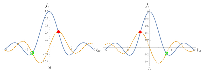
Figure 3: Graphical illustration of the solutions to the eigenvalue equation of Eq. (92) for a ground-state (a) quark, which has $k=-1$, and (b) antiquark, which has $k=1$. Note that the solid curve denotes $j_{0}$ in each case, whereas the dashed line is ${j_{1}}/{\epsilon_{\alpha}}$ in (a) and ${-j_{1}}/{\epsilon_{\alpha}}$ in (b). The solid red dot shows the proper solution in each case.

- (1) S. Weinberg, “Baryon and lepton-nonconserving processes,” Phys. Rev. Lett. 43 (1979) 1566.
- (2) J. Schechter and J. W. Valle, “Neutrino decay and spontaneous violation of lepton number,” Phys. Rev. D 25 (1982) 774.
- (3) J. Schechter and J. W. Valle, “Neutrinoless double- decay in SU(2)U(1) theories,” Phys. Rev. D25 (1982) 2951.
- (4) R. N. Mohapatra and R. E. Marshak, “Local B-L symmetry of electroweak interactions, Majorana neutrinos, and neutron oscillations,” Phys. Rev. Lett. 44 (1980) 1316.
- (5) R. N. Mohapatra and R. E. Marshak, “Phenomenology of neutron oscillations,” Phys. Lett. B 94 (1980) 183–186.
- (6) V. A. Kuzmin, “CP violation and baryon asymmetry of the universe,” Pisma Zh. Eksp. Teor. Fiz. 12 (1970) 228.
- (7) S. L. Glashow, “Overview,” in Proceedings of Neutrino ’79 (1979) p. 518.
- (8) R. Cowsik and S. Nussinov, “Some constraints on B= 2 - oscillations,” Phys. Lett. B 101 (1981) 237–240.
- (9) M. Baldo-Ceolin et al., “A new experimental limit on neutron-antineutron oscillations,” Z. Phys. C 63 (1994) 409–416.
- (10) D. Phillips et al., “Neutron-antineutron oscillations: Theoretical status and experimental prospects,” Phys. Rept. 612 (2016) 1–45.
- (11) D. Milstead, “A new high sensitivity search for neutron-antineutron oscillations at the ESS,” 1510.01569 [physics.ins-det].
- (12) K. Abe et al. [Super-Kamiokande Collaboration], “The Search for oscillation in Super-Kamiokande I,” Phys. Rev. D91 (2015) 072006, arXiv:1109.4227 [hep-ex].
- (13) C. B. Dover, A. Gal, and J. M. Richard, “Neutron anti-neutron oscillations in nuclei,” Phys. Rev. D27 (1983) 1090–1100.
- (14) E. Friedman and A. Gal, “Realistic calculations of nuclear disappearance lifetimes induced by n anti-n oscillations,” Phys. Rev. D78 (2008) 016002, arXiv:0803.3696 [hep-ph].
- (15) B. Aharmim et al. [SNO Collaboration], “The search for neutron-antineutron oscillations at the Sudbury Neutrino Observatory,” arXiv:1705.00696 [hep-ex].
- (16) V. Kopeliovich and I. Potashnikova, “Restriction on the Neutron-Antineutron Oscillations from the SNO Data on the Deuteron Stability,” JETP Lett. 95 (2012) 1–5, arXiv:1112.3549 [hep-ph] [Zh. Eksp. Teor. Fiz.95, 3 (2012)].
- (17) B. O. Kerbikov, “Quantum damping of neutron-antineutron oscillations,” arXiv:1704.07117 [hep-ph].
- (18) R. N. Mohapatra, “Theory and phenomenology of neutron - anti-neutron oscillation,” in Workshop on Neutrino-Antineutrino Oscillations Cambridge, Mass., April 30-May 1, 1982 (1982).
- (19) P. Kabir, “Limits on - oscillations,” Phys. Rev. Lett. 51 (1983) 231.
- (20) J. Basecq and L. Wolfenstein, “B= 2 transitions,” Nucl. Phys. B 224 (1983) 21–31.
- (21) J. M. Arnold, B. Fornal, and M. B. Wise, “Simplified models with baryon number violation but no proton decay,” Phys. Rev. D 87 (2013) 075004.
- (22) C. Berger et al., “Lifetime limits on (B-L)-violating nucleon decay and di-nucleon decay modes from the Fréjus experiment,” Phys. Lett. B 269 (1991) 227–233.
- (23) R. Bernabei et al., “Search for the nucleon and di-nucleon decay into invisible channels,” Phys. Lett. B 493 (2000) 12–18.
- (24) M. Litos et al., “Search for dinucleon decay into kaons in Super-Kamiokande,” Phys. Rev. Lett. 112 (2014) 131803.
- (25) J. Gustafson et al., “Search for dinucleon decay into pions at Super-Kamiokande,” Phys. Rev. D 91 (2015) 072009.
- (26) Z. Chacko and R. N. Mohapatra, “Supersymmetric SU(2)SU(2)SU(4)c and observable neutron-antineutron oscillations,” Phys. Rev. D 59 (1999) 055004.
- (27) K. Babu and R. N. Mohapatra, “Observable neutron–antineutron oscillations in seesaw models of neutrino mass,” Phys. Lett. B 518 (2001) 269–275.
- (28) K. Babu and R. N. Mohapatra, “Determining Majorana nature of neutrino from nucleon decays and - oscillations,” Phys. Rev. D 91 (2015) 013008.
- (29) K. Babu, P. B. Dev, and R. Mohapatra, “Neutrino mass hierarchy, neutron-antineutron oscillation from baryogenesis,” Phys. Rev. D 79 (2009) 015017.
- (30) K. Babu and R. Mohapatra, “Coupling unification, GUT scale baryogenesis and neutron–antineutron oscillation in so (10),” Phys. Lett. B 715 (2012) 328–334.
- (31) K. Babu, P. B. Dev, E. C. Fortes, and R. Mohapatra, “Post-sphaleron baryogenesis and an upper limit on the neutron-antineutron oscillation time,” Phys. Rev. D 87 (2013) 115019.
- (32) S. Gardner and E. Jafari, “Phenomenology of - oscillations revisited,” Phys. Rev. D 91 (2015) 096010.
- (33) A. Chodos, R. L. Jaffe, K. Johnson, and C. B. Thorn, “Baryon Structure in the Bag Theory,” Phys. Rev. D10 (1974) 2599.
- (34) A. Chodos, R. L. Jaffe, K. Johnson, C. B. Thorn, and V. F. Weisskopf, “A New Extended Model of Hadrons,” Phys. Rev. D9 (1974) 3471–3495.
- (35) S. Gardner and X. Yan, “Neutron-antineutron conversion to search for B-L violation.” arXiv:1711.xxxx, in preparation.
- (36) S. Gardner and X. Yan, “CPT, CP, and C transformations of fermions, and their consequences, in theories with B-L violation,” Phys. Rev. D 93 (2016) 096008.
- (37) B. Kayser and A. S. Goldhaber, “CPT and CP Properties of Majorana Particles, and the Consequences,” Phys. Rev. D28 (1983) 2341.
- (38) B. Kayser, “CPT, CP, and C Phases and their Effects in Majorana Particle Processes,” Phys. Rev. D30 (1984) 1023.
- (39) G. Feinberg and S. Weinberg, “On the phase factors in inversions,” Nuovo Cim. 14 (1959) 571–592.
- (40) P. A. Carruthers, Spin and Isospin in Particle Physics. Gordon & Breach, New York, USA (1971).
- (41) W. C. Haxton and G. J. Stephenson, “Double Beta Decay,” Prog. Part. Nucl. Phys. 12 (1984) 409–479.
- (42) L. Wolfenstein, “Different Varieties of Massive Dirac Neutrinos,” Nucl. Phys. B186 (1981) 147–152.
- (43) Z. Berezhiani and A. Vainshtein, “Neutron-Antineutron Oscillation as a Signal of CP Violation,” arXiv:1506.05096 [hep-ph].
- (44) K. Fujikawa and A. Tureanu, “Parity-doublet representation of Majorana fermions and neutron oscillation,” Phys. Rev. D94 (2016) no. 11, 115009, arXiv:1609.03203 [hep-ph].
- (45) S. Rao and R. E. Shrock, “Six Fermion () Violating Operators of Arbitrary Generational Structure,” Nucl. Phys. B232 (1984) 143–179.
- (46) S. Rao and R. Shrock, “ Transition Operators and Their Matrix Elements in the MIT Bag Model,” Phys. Lett. 116B (1982) 238–242.
- (47) W. E. Caswell, J. Milutinovic, and G. Senjanovic, “Matter-antimatter transition operators: a manual for modeling,” Phys. Lett. 122B (1983) 373–377.
- (48) M. I. Buchoff, C. Schroeder, and J. Wasem, “Neutron-antineutron oscillations on the lattice,” PoS LATTICE2012 (2012) 128, arXiv:1207.3832 [hep-lat].
- (49) S. Syritsyn, M. I. Buchoff, C. Schroeder, and J. Wasem, “Neutron-antineutron oscillation matrix elements with domain wall fermions at the physical point,” PoS LATTICE2015 (2016) 132.
- (50) M. E. Peskin and D. V. Schroeder, An Introduction to Quantum Field Theory. Addison-Wesley, Reading, USA, 1995. http://www.slac.stanford.edu/~mpeskin/QFT.html.
- (51) A. Hayreter and G. Valencia, “LHC constraints on color octet scalars,” Phys. Rev. D96 (2017) 035004, arXiv:1703.04164 [hep-ph].
- (52) R. C. Fernow, Introduction to Experimental Particle Physics. Cambridge University Press, Cambridge, UK 1986.
- (53) R. Corliss [DarkLight Collaboration], “Searching for a dark photon with DarkLight,” Nucl. Instrum. Meth. A865 (2017) 125–127.
- (54) R. Alarcon et al., “Measured radiation and background levels during transmission of megawatt electron beams through millimeter apertures,” Nucl. Instrum. Meth. A729 (2013) 233–240, arXiv:1305.7215 [physics.acc-ph].
- (55) G. R. Neil et al., “The JLab high power ERL light source,” Nucl. Instrum. Meth. A557 (2006) 9–15.
- (56) T. M. Ito et al. [SAMPLE Collaboration], “Parity violating electron deuteron scattering and the proton’s neutral weak axial vector form-factor,” Phys. Rev. Lett. 92 (2004) 102003, arXiv:nucl-ex/0310001 [nucl-ex].
- (57) T. Allison et al. [Qweak Collaboration], “The Qweak experimental apparatus,” Nucl. Instrum. Meth. A781 (2015) 105–133, arXiv:1409.7100 [physics.ins-det].
- (58) K. Clusius and E. Bartholome, “Calorische und Thermische Eigenschaften des Kondensierten Schweren Wasserstoffs,” Z. physik. Chem. B30 (1935) 237–57.
- (59) E. T. Jurney, P. J. Bendt, and J. C. Browne, “Thermal neutron capture cross section of deuterium,” Phys. Rev. C25 (1982) 2810–2811.
- (60) L. Brillouin, “A Theorem of Larmor and Its Importance for Electrons in Magnetic Fields,” Phys.Rev. 67 (1945) 260.
- (61) J. D. Bowman and V. Gudkov, “Search for time reversal invariance violation in neutron transmission,” Phys. Rev. C90 (2014) 065503, arXiv:1407.7004 [hep-ph].
- (62) N. P. Luciano, A High-Energy Neutron Flux Spectra Measurement Method for the Spallation Neutron Source. Master’s Thesis, University of Tennessee. 2012. http://trace.tennessee.edu/utk_gradthes/1178.
- (63) H. M. Roder, “The molar volume (density) of solid oxygen in equilibrium with vapor,”Journal of Physical and Chemical Reference Data 7 (1978) 949–958.
- (64) https://ncnr.nist.gov/equipment/msnews/ncnr/vsans.html.
- (65) J. C. Cook, “Design and estimated performance of a new neutron guide system for the NCNR expansion project,” Rev. Sci. Instr. 80 (2009) 023101–023101–10.
- (66) R. E. Shrock and S. B. Treiman, “ Transition Amplitude in the MIT Bag Model,” Phys. Rev. D19 (1979) 2148–2157.
- (67) X.-W. Kang, H.-B. Li, and G.-R. Lu, “Study of - Oscillation in quantum coherent state by using decay,” Phys. Rev. D81 (2010) 051901, arXiv:0906.0230 [hep-ph].
- (68) A. Addazi, X.-W. Kang, and M. Yu. Khlopov, “Testing B-violating signatures from exotic instantons in future colliders,” Chin. Phys. C41 (2017) 093102, arXiv:1705.03622 [hep-ph].
- (69) J. Pasupathy, “The neutron-antineutron transition amplitude in the MIT bag model,” Phys. Lett. B 114 (1982) 172–174.