In this paper, spatially homogeneous and anisotropic Bianchi type-I cosmological models of Brans-Dicke theory of gravitation are investigated. The model represents accelerating universe at present and is considered to be dominated by dark energy. Cosmological constant $\Lambda$ is considered as a candidate for the dark energy that has negative pressure and is responsible for the present acceleration. The derived model agrees at par with the recent SN Ia observations. We have set BD-coupling constant $\omega$ to be  $40000$,  seeing the solar system tests and evidences. We have discussed the various physical and geometrical properties of the models and have compared them with the corresponding relativistic models.
Keywords: Bianchi type-I $\Lambda$ Dominated universe, Dark energy, BD-theory, Accelerating universe
PACS: 98.80.-k

1 INTRODUCTION

Type Ia supernovae observations [1, 2], the observations of CMBR anisotropy spectrum [3], large scale structure (LSS) [4] and Planck results for CMB anisotropies [5] ascertain the fact that our universe is undergoing an accelerated expansion at present. It is considered to be dominated by dark energy that has negative pressure and is responsible for the present acceleration. As it is a well known fact that the universe had once gone through accelerated phase during inflation for a very short period, so the present phase may be the second attempt for it to have gone through accelerated phase. The large-scale structure surveys and results of measurements of masses of galaxies [6] provide the best fit value of density parameter for matter $\Omega_{m,0}=0.3$ and consequently $\Omega_{\Lambda,0}=0.7$. These researches and the latest observations explores that our universe is nearly flat.
The present scenario of accelerating phase of the universe and the various observational cosmological facts regarding the present day universe are very well explained by the $\Lambda$-cold dark matter ($\Lambda$-CDM) cosmological model [7, 8]. In this model, Einstein’s field equations are solved for Friedmann Robertson Walker (FRW) metric in presence of positive cosmological constant as source for dark energy along with perfect fluid distribution of the matter. It is a beauty of the $\Lambda$-CDM model that the specific value of cosmological constant changes the decelerating phase of the universe into the accelerating one. The latest cosmological observations [9, 10] agrees with $\Lambda$-CDM model.
Spatially homogeneous and anisotropic cosmology had been a matter of interest to the cosmologist long back since 1962, when Heckmann and Schucking [11] wrote a chapter on anisotropic Universe. The spatially homogeneous and anisotropic Bianchi type-I metric is often referred as Heckmann Schuking metric. It was thought that neutrino viscosity in the primordial fire ball [12, 13] may create anisotropy in the Universe which dissipates out with the advent of time. Accordingly a large number of spatially homogeneous and anisotropic solutions of Einstein’s theory have been obtained [14]-[24]. Off late Wilkinson Microwave Anisotropic Probe (Bennett et al. [25]) also created interest in the investigation of anisotropic models of the universe. Recently, Goswami et al. [26]-[30] have also developed $\Lambda$-CDM type models for Bianchi type-I anisotropic universe.
The fundamental and the basic philosophy behind the general theory of relativity (GTR)is that the presence of gravitational field geometrizes the space-time. Einstein was very much impressed by the Mach philosophy that the distant background of the universe has the impact with the local matter and that the inertial property in the matter is due to its intersection with the distant matter. But the trouble in GTR is that it does not incorporate fully Mach’s principle [31]. A modified relativistic theory of gravitation, closely related to Jordan’s theory [32] and compatible to Mach’s principle was developed by Brans and Dicke in 1961, well known as Brans-Dicke gravity [33, 34]. The constant coupling parameter $\omega$ and a scalar field $\phi$ provide the intersection with the distant background of the universe. The recent experimental evidences [35]$-$[38] indicate that the value for coupling constant $\omega$ must be higher than 40000. It is found that Brans-Dicke theory goes over to GTR when $\omega$ goes to infinity [31]. Low energy limit of many theories of quantum gravity (for example, superstring theory, etc.) and the cosmology have been discussed in BD-theory by many authors [39, 40, 41]. So many researchers (see [42]-[56] and references therein) discussed the various burning issues like all important features of the evolution of the universe such as: inflation, early and late time behaviour of the universe, cosmic acceleration and structure formation, quintessence and coincidence problem, self-interacting potential and cosmic acceleration, high energy description of dark energy in an approximate 3-brane in Brans-Dicke theory.
In view of above ideas, it is worth to find out effect of cosmological constant $\Lambda$ in BD-theory of gravitation, so that we could get history of evolution of the universe that also contain the present accelerated phase. Earlier, Hrycyna and Lowski [57] studied dynamical evolution of the universe in BD-theory and compared their outcome with the corresponding results of relativistic cosmology. Dieter Lorenz-Petzold [58] obtained Bianchi type-I BD-exact solution. Recently, M. Sharif and S. Waheed [59] and Y. Kucukakca et. al.[60] have developed anisotropic universe models in Brans–Dicke theory. Maurya et al.[61] obtained anisotropic string cosmological models in Brans-Dicke theory of gravitation with time dependent deceleration parameter. Off late, Goswami [62] has developed a $\Lambda$-CDM type cosmological model in BD-theory and has obtained a spatially flat dust filled universe in the presence of a positive cosmological constant $\Lambda$.
In this paper, we have investigated spatially homogeneous and anisotropic Bianchi type-I cosmological models in Brans-Dicke theory of gravitation. Although the format of the paper is similar to that of Goswami [62], yet it is a different work. Goswami [62] has considered a spatially flat dust filled isotropic universe where as our case is that of a spatially flat dust filled anisotropic universe. The reason for taking anisotropy is explained above. The outline of paper is as follows: in Section $2$, Brans-Dicke field equations for Bianchi type-I metric are obtained. In Section $3$, we have developed a linear relationship amongst energy parameters $\Omega_{m}$, $\Omega_{\Lambda}$ and $\Omega_{\sigma}$. Section $4$ discusses variation of gravitational constant with red shift. In Section $5$, we have obtained expressions for Hubble’s constant, luminosity distance and apparent magnitude. We have also estimated the present values of energy parameters and Hubble’s constant. The deceleration parameter (DP), age of the universe and certain physical properties of the universe are presented in Section $6$. Finally, conclusions are summarized in Section $7$.

2 BRANS-DICKE FIELD EQUATIONS FOR BIANCHI TYPE I METRIC

We consider a spatially homogeneous and anisotropic Bianchi type 1 space-time given by following metric

$$ds^{2}=c^{2}dt^{2}-A^{2}dx^{2}-B^{2}dy^{2}-C^{2}dz^{2},$$ (1)

where $A(t)$, $B(t)$ and $C(t)$ are scale factors along $x$, $y$ and $z$ axes.

The energy momentum tensor is taken as that of perfect fluid given by following metric

$$T_{ij}=(p+\rho)u_{i}u_{j}-pg_{ij},$$ (2)

where $g_{ij}u^{i}u^{j}=1$ and $u^{i}$ is the 4-velocity vector.

In co-moving co-ordinates

$$u^{\alpha}=0,~{}~{}~{}~{}~{}~{}~{}~{}~{}\alpha=1,2,3.$$

The Brans-Dicke [33] field equations are derived from a variational principle with a Lagrangian that generalizes the traditional one; we have included in the Brans-Dicke Lagrangian the cosmological constant for generality (see Petrosian [63]). Brans-Dicke field equations with cosmological constant $\Lambda$ are obtained from following action [64]

$$S=\int\sqrt{-g}\left\{\phi\left(R-2\Lambda\right)+\omega\frac{\phi_{k}\phi^{k}}{\phi}+\frac{16\pi L_{M}}{c^{4}}\right\}d^{4}x,$$ (3)

where $\phi$ is the scalar field representing reciprocal of varying Gravitational constant $G$, $\phi_{,i}\equiv\phi_{i}$, R is Ricci scalar and $L_{M}$ is the matter Lagrangian.

The field equations are obtained by varying the action with respect to $g_{ij}$ and $\phi$ as independent variables. The Brans-Dicke field equations with cosmological constant $\Lambda$ are given as follows:

$$R_{ij}-\frac{1}{2}R+\Lambda g_{ij}=-\frac{8\pi}{\phi c^{4}}T_{ij}-\frac{\omega}{\phi^{2}}\left(\phi_{i}\phi_{j}-\frac{1}{2}g_{ij}\phi_{k}\phi^{k}\right)-\frac{1}{\phi}\left(\phi_{i;j}-g_{ij}\Box\phi\right),$$ (4)

$$(2\omega+3)\Box\phi=\frac{8\pi T}{c^{4}}+2\Lambda\phi,$$ (5)

where $\Box\phi=\phi^{i}_{;i}$.

Choosing co-moving coordinates, the field Eqs. (4) and (5), for the line element (1), are obtained as

$$\frac{\ddot{B}}{B}+\frac{\ddot{C}}{C}+\frac{\dot{B}\dot{C}}{BC}=-\frac{8\pi}{\phi c^{2}}p-\frac{\omega\dot{\phi}^{2}}{2\phi^{2}}-\frac{\dot{\phi}}{\phi}(\frac{\dot{B}}{B}+\frac{\dot{C}}{C})-\frac{\ddot{\phi}}{\phi}+\Lambda c^{2},$$ (6)

$$\frac{\ddot{A}}{A}+\frac{\ddot{C}}{C}+\frac{\dot{A}\dot{C}}{AC}=-\frac{8\pi}{\phi c^{2}}p-\frac{\omega\dot{\phi}^{2}}{2\phi^{2}}-\frac{\dot{\phi}}{\phi}(\frac{\dot{A}}{A}+\frac{\dot{C}}{C})-\frac{\ddot{\phi}}{\phi}+\Lambda c^{2},$$ (7)

$$\frac{\ddot{A}}{A}+\frac{\ddot{B}}{B}+\frac{\dot{A}\dot{B}}{AB}=-\frac{8\pi}{\phi c^{2}}p-\frac{\omega\dot{\phi}^{2}}{2\phi^{2}}-\frac{\dot{\phi}}{\phi}(\frac{\dot{A}}{A}+\frac{\dot{B}}{B})-\frac{\ddot{\phi}}{\phi}+\Lambda c^{2},$$ (8)

$$\frac{\dot{A}\dot{B}}{AB}+\frac{\dot{B}\dot{C}}{BC}+\frac{\dot{C}\dot{A}}{AC}=\frac{8\pi}{\phi c^{2}}\rho-\frac{\dot{\phi}}{\phi}(\frac{\dot{A}}{A}+\frac{\dot{B}}{B}+\frac{\dot{C}}{C})+\frac{\omega\dot{\phi}^{2}}{2\phi^{2}}+\Lambda c^{2},$$ (9)

$$\frac{\ddot{\phi}}{\phi}+\frac{\dot{\phi}}{\phi}(\frac{\dot{A}}{A}+\frac{\dot{B}}{B}+\frac{\dot{C}}{C})=\frac{8\pi(\rho-3p)}{(2\omega+3)c^{2}\phi}+\frac{2\Lambda c^{2}}{2\omega+3},$$ (10)

$$\frac{\dot{\rho}}{\rho}+\gamma\frac{\dot{(ABC)}}{ABC}=0\;.$$ (11)

Here Eq. (11) corresponds to energy conservation equation $T^{ij}_{;j}$ and $p=(\gamma-1)\rho$ is equation of state. $\gamma=1$ for dust dominated universe and $\gamma=4/3$ for radiation filled universe. Subtracting Eq. (6) from Eq.(7), Eq.(7) from Eq.(8) and Eq.(6) from Eq. (8), we obtain

$$\frac{\ddot{A}}{A}-\frac{\ddot{B}}{B}+\left(\frac{\dot{A}}{A}-\frac{\dot{B}}{B}\right)\left(\frac{\dot{C}}{C}+\frac{\dot{\phi}}{\phi}\right)=0,$$ (12)

$$\frac{\ddot{B}}{B}-\frac{\ddot{C}}{C}+\left(\frac{\dot{B}}{B}-\frac{\dot{C}}{C}\right)\left(\frac{\dot{A}}{A}+\frac{\dot{\phi}}{\phi}\right)=0,$$ (13)

$$\frac{\ddot{C}}{C}-\frac{\ddot{A}}{A}+\left(\frac{\dot{C}}{C}-\frac{\dot{A}}{A}\right)\left(\frac{\dot{B}}{B}+\frac{\dot{\phi}}{\phi}\right)=0.$$ (14)

Subtracting Eq.(14) from Eq.(12), we get

$$\frac{\ddot{B}}{B}+\frac{\ddot{C}}{C}+\frac{2\dot{B}\dot{C}}{BC}+\left(\frac{\dot{B}}{B}+\frac{\dot{C}}{C}\right)\frac{\dot{\phi}}{\phi}=2\frac{\ddot{A}}{A}+\left(\frac{\dot{B}}{B}+\frac{\dot{C}}{C}\right)\frac{\dot{A}}{A}+\frac{2\dot{A}}{A}\frac{\dot{\phi}}{\phi}.$$ (15)

This equation can be re-written in the following form

$$\frac{d}{dt}\left(\frac{\dot{(BC)}}{BC}\right)+\left(\frac{\dot{(BC)}}{BC}\right)^{2}+\left(\frac{\dot{(BC)}}{BC}-2\frac{\dot{(A)}}{A}\right)\frac{\dot{(\phi)}}{\phi}=2\frac{d}{dt}\left(\frac{\dot{A}}{A}\right)+2\frac{\dot{A}^{2}}{A^{2}}+\frac{\dot{A}\dot{(BC)}}{ABC}.$$ (16)

Integrating this equation, we get the following first integral

$$\left(\frac{\dot{(BC)}}{BC}-\frac{2\dot{A}}{A}\right)\times(ABC\phi)=L,$$ (17)

where $L$ is constant of integration.

The observations show that the anisotropy existing in the past dissipates out at present. So we take constant $L=0$. This gives the following relationship amongst the metric coefficients

$$A^{2}=BC\;.$$ (18)

Therefore, we may assume

$$B=Ad\;\;\&\;\;C=\frac{A}{d},$$ (19)

where  d = d(t).
With these choices of metric coefficients, the Brans-Dicke field equations take the following form

$$2{\left(\frac{\ddot{A}}{A}\right)}+\left(\frac{\dot{A}}{A}\right)^{2}+\frac{\omega\dot{\phi}^{2}}{2\phi^{2}}+2\frac{\dot{\phi}}{\phi}\frac{\dot{A}}{A}+\frac{\ddot{\phi}}{\phi}=-\frac{8\pi}{\phi c^{2}}p-{\left(\frac{\dot{d}}{d}\right)}^{2}+\Lambda c^{2},$$ (20)

$$\left(\frac{\dot{A}}{A}\right)^{2}+\frac{\dot{\phi}}{\phi}\frac{\dot{A}}{A}-\frac{\omega\dot{\phi}^{2}}{6\phi^{2}}=\frac{8\pi}{3\phi c^{2}}\rho+\frac{\Lambda c^{2}}{3}+\frac{1}{3}{\left(\frac{\dot{d}}{d}\right)}^{2},$$ (21)

$$\frac{d}{dt}\left(\frac{\dot{d}}{d}\right)+\frac{\dot{d}}{d}\left(3\frac{\dot{A}}{A}+\frac{\dot{\phi}}{\phi}\right)=0$$ (22)

$$\frac{\ddot{\phi}}{\phi}+3\frac{\dot{A}}{A}\frac{\dot{\phi}}{\phi}=\frac{8\pi(\rho-3p)}{(2\omega+3)c^{2}\phi}+\frac{2\Lambda c^{2}}{2\omega+3}\;.$$ (23)

$$\frac{\dot{\rho}}{\rho}+3\gamma\frac{\dot{A}}{A}=0.$$ (24)

The equation (22) is integrable and provides following solution

$$\frac{\dot{d}}{d}=\frac{k}{A^{3}\phi},$$ (25)

where k is constant of integration
Here we note that when the constant k=0, parameter d=0 and this yields the metric coefficients

$$A=B=C$$

In this case our model is converted to homogeneous and isotropic BD- model derived by Goswami [62].
So for anisotropic universe $k\neq 0$

3 ENERGY PARAMETERS AND THEIR RELATIONSHIP FOR DUST FILLED UNIVERSE

The universe is as at present dust dominated, so we consider $p=0$ and $\gamma=1$. Since the right hand side of Eq. (21) are energy densities, we define energy parameters for matter, dark energy and anisotropic energy as follows.

$$\Omega_{m}=\frac{8\pi\rho}{3c^{2}H^{2}\phi},\;\;\Omega_{\Lambda}=\frac{\Lambda c^{2}}{3H^{2}},and\;\;\Omega_{\sigma}=\frac{k^{2}}{3H^{2}A^{6}\phi^{2}}\;.$$ (26)

We also define decelerating parameter for scale factor $a$ and scalar field $\phi$ as

$$q=-\frac{\ddot{A}}{AH^{2}}\;and\;q_{\phi}=-\frac{\ddot{\phi}}{\phi H^{2}}\;,$$ (27)

where the Hubble Constant

$$H=\frac{\dot{A}}{A}$$

Therefore, with the help of Eqs. (26) and (27), Eqs. (20) to (23) are reduced to

$$-2q+1+\frac{\omega\xi^{2}}{2}+2\xi-q_{\phi}=3\Omega_{\Lambda}-3\Omega_{\sigma},$$ (28)

$$\Omega_{m}+\Omega_{\Lambda}+\Omega_{\sigma}=1+\xi-\frac{\omega}{6}\xi^{2},$$ (29)

$$-q_{\phi}+3\xi=\frac{3\Omega_{m}}{2\omega+3}+\frac{6\Omega_{\Lambda}}{2\omega+3},$$ (30)

$$\xi=\frac{\dot{\phi}}{H\phi}.$$ (31)

The Eqs. (28)-(31) give rise to the following equation.

$$q-(\omega+1)q_{\phi}+(3\omega+2)\xi=2\;,$$ (32)

which has first integral as

$$(\omega+1)\frac{\dot{\phi}}{\phi}-\frac{\dot{A}}{A}=\frac{L}{\phi A^{3}},$$ (33)

where $L$ is constant of integration. The solution Eq.(33) has a singularity at $A=0\ and\ \phi=0$, so we take constant $L=0$. This gives the following power law relation between scalar field $\phi$ and scale factor$\;A$.

$$\xi=\frac{1}{\omega+1},~{}~{}\phi=\phi_{0}\left(\frac{A}{A_{0}}\right)^{\frac{1}{\omega+1}},$$ (34)

where $\phi_{0}$ and $A_{0}$ are values of scalar field $\phi$ and scale factors $A$ at present. Putting value of $\xi$ in Eq. (29), we get following relationship amongst energy parameters.

$$\Omega_{m}+\Omega_{\Lambda}+\Omega_{\sigma}=1+\frac{5\omega+6}{6(\omega+1)^{2}}\;.$$ (35)

This result is analogue of the relativistic result obtained by us in [26] in Brans-Dicke theory. The relativistic result is as follows

$$\Omega_{m}+\Omega_{\Lambda}+\Omega_{\sigma}=1\;.$$ (36)

4 GRAVITATIONAL CONSTANT VERSUS REDSHIFT RELATION

As gravitational constant $G$ is reciprocal of $\phi$ i.e.

$$G=\frac{1}{\phi}\;,$$ (37)

and

$$\frac{A_{0}}{A}=(1+z),$$ (38)

where $z$ is the red shift.

So, from Eqs. (34), (37) and (38), we obtain

$$\frac{{G}}{G_{0}}=\left(1+z\right)^{\frac{1}{\omega+1}}.$$ (39)

This result had been obtained earlier by Goswami [62] for spatially flat dust filled BD-universe. It is concluded that variation of gravitational constant G over red shift z and coupling constant $\omega$ follows same pattern for both isotropic and anisotropic BD-universe.
This relation ship shows that $G$ grows toward the past and in fact it diverges at cosmological singularity. Radar observations, Lunar mean motion and the Viking landers on Mars [35] suggest that rate of variation of gravitational constant must be very much slow of order $10^{-12}year^{-1}$. The recent experimental evidence [37, 38] shows that $\omega>40000$. Accordingly, we consider large coupling constant $\omega=40000$ in this study.

From Eqs. (33) and (37), the present rate of gravitational constant is calculated as

$$\left(\frac{\dot{G}}{G}\right)_{0}=-\frac{1}{\omega+1}H_{0}\;,$$ (40)

where $H_{0}\simeq 10^{-10}year^{-1}$.

Eq. (39) exhibits the fact that how $G/G_{0}$ varies over $\omega$. For higher values of $\omega$, $G/G_{0}$ grows very slow over redshift, where as for lower values of $\omega$ it grows fast. The variation of Gravitational constant over red shift for different $\omega$’s is already shown in fig.(1) of ref. [62].

5 EXPRESSIONS FOR HUBBLE’S CONSTANT, LUMINOSITY DISTANCE AND APPARENT MAGNITUDE

5.1 HUBBLE’S CONSTANT

The energy conservation Eq. (24) is integrable for dust filled universe, giving rise to following expression amongst matter density $\rho$, average scale factor $a$ and the red shift $z$ of the universe

$$\rho=(\rho)_{0}\left(\dfrac{A_{0}}{A}\right)^{3}=(\rho)_{0}\left(1+z\right)^{3}.$$ (41)

where we have used the relation given by the Eq. (38).

Now, using Eqs. (26), (35), (38) and (41), we get following expressions for Hubble’s constant in terms of scale factor and redshift

$$H=\frac{H_{0}}{\sqrt{1+\frac{5\omega+6}{6(\omega+1)^{2}}}}\sqrt{(\Omega_{m})_{0}\left(\frac{A_{0}}{A}\right)^{\frac{3\omega+4}{\omega+1}}+(\Omega_{\sigma})_{0}\left(\frac{A_{0}}{A}\right)^{2\left(\frac{3\omega+4}{\omega+1}\right)}+(\Omega_{\Lambda})_{0}}\,,$$ (42)

and

$$H=\frac{H_{0}}{\sqrt{1+\frac{5\omega+6}{6(\omega+1)^{2}}}}\sqrt{(\Omega_{m})_{0}(1+z)^{\frac{3\omega+4}{\omega+1}}+(\Omega_{\sigma})_{0}(1+z)^{2\left(\frac{3\omega+4}{\omega+1}\right)}+(\Omega_{\Lambda})_{0}}\,,$$ (43)

respectively.

5.2 LUMINOSITY DISTANCE

The luminosity distance which determines flux of the source is given by

$$D_{L}=A_{0}r(1+z),$$ (44)

where $r$ is the spatial co-ordinate distance of a source. The luminosity distance for metric (1) can be written as [26]

$$D_{L}=c(1+z)\int^{z}_{0}\frac{dz}{H(z)}.$$ (45)

Therefore, by using Eq. (43), the luminosity distance $D_{L}$ for our model is obtained as

$$D_{L}=\frac{c(1+z)\sqrt{1+\frac{5\omega+6}{6(\omega+1)^{2}}}}{H_{0}}\int_{0}^{z}\frac{dz}{\sqrt{[(\Omega_{m})_{0}(1+z)^{\frac{3\omega+4}{\omega+1}}+(\Omega_{\sigma})_{0}(1+z)^{2\left(\frac{3\omega+4}{\omega+1}\right)}+(\Omega_{\Lambda})_{0}]}}\,.$$ (46)

5.3 APPARENT MAGNITUDE

The apparent magnitude of a source of light is related to the luminosity distance via following expression

$$m=16.08+5log_{10}\frac{H_{0}D_{L}}{.026cMpc}.$$ (47)

Using Eq. (46), we get following expression for apparent magnitude in our model

$$m=16.08+5log_{10}\left(\frac{(1+z)\sqrt{1+\frac{5\omega+6}{6(\omega+1)^{2}}}}{.026}\int_{0}^{z}\frac{dz}{\sqrt{[(\Omega_{m})_{0}(1+z)^{\frac{3\omega+4}{\omega+1}}+(\Omega_{\sigma})_{0}(1+z)^{2\left(\frac{3\omega+4}{\omega+1}\right)}+(\Omega_{\Lambda})_{0}]}}\right).$$ (48)

5.4 ENERGY PARAMETERS AT PRESENT

We consider $287$ high red shift ($0.3\leq z\leq 1.4$ ) SN Ia supernova data set of observed apparent magnitudes along with their possible error from union $2.1$ compilation [65]. In our early work [26] $-$ [30], we have presented a technique to estimate the present values of energy parameters $(\Omega_{m})_{0}$, $(\Omega_{\Lambda})_{0}$, and $(\Omega_{\sigma})_{0}$ by comparing the theoretical and observed results with the help of following $\chi^{2}$ formula.

$$\chi_{SN}^{2}=X-\frac{Y^{2}}{Z}+log_{10}\left(\frac{Z}{2\pi}\right),$$ (49)

where

$$X=\overset{287}{\underset{i=1}{\sum}}\frac{\left[\left(m\right)_{ob}-\left(m\right)_{th}\right]^{2}}{\sigma_{i}^{2}},$$ (50)

$$Y=\overset{287}{\underset{i=1}{\sum}}\frac{\left[\left(m\right)_{ob}-\left(m\right)_{th}\right]}{\sigma_{i}^{2}},$$ (51)

and

$$Z=\overset{287}{\underset{i=1}{\sum}}\frac{1}{\sigma_{i}^{2}}.$$ (52)

Here the sums are taken over data sets of observed and theoretical values of apparent magnitude of $287$ supernovae.

On the basis of minimum value of $\chi^{2}$, we get the best fit present values of $\Omega_{m}$ and $\Omega_{\Lambda}$. For this, the present anisotropic energy density $(\Omega_{\sigma})$ is taken to be very small i. e. $\Omega_{\sigma}$ = 0.0002, coupling constant $\omega$ is taken as $40000$ and the theoretical values are calculated from Eq. (48). We have found that the best fit present values of $\Omega_{m}$ and $\Omega_{\Lambda}$ are $(\Omega_{m})_{0}=0.294$ and $(\Omega_{\Lambda})_{0}=0.7058$ for minimum $\chi^{2}=0.6544$.

The Figures $1$ and $2$ indicate how the observed values of apparent magnitudes and luminosity distances reach close to the theoretical graphs for $(\Omega_{\Lambda})_{0}$ = 0.7058, $(\Omega_{m})_{0}=0.294$ and $(\Omega_{\sigma})_{0}=0.0002$.

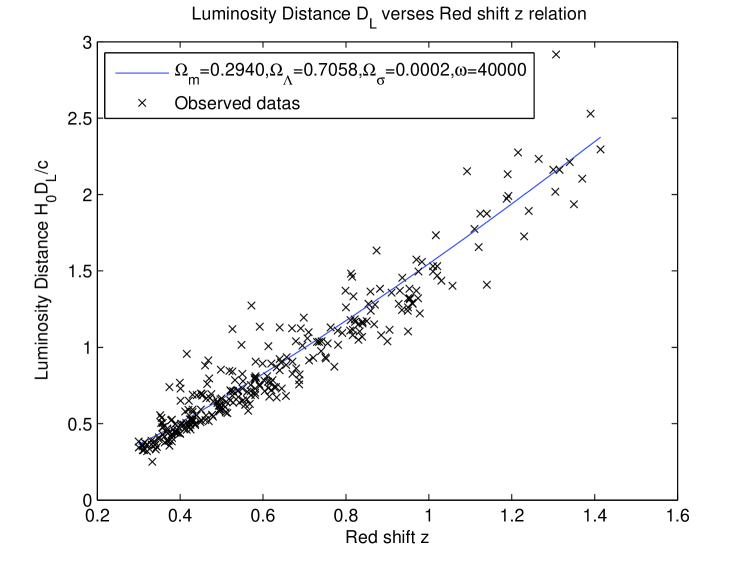
Figure 1: Luminosity distance versus red shift best fit curve

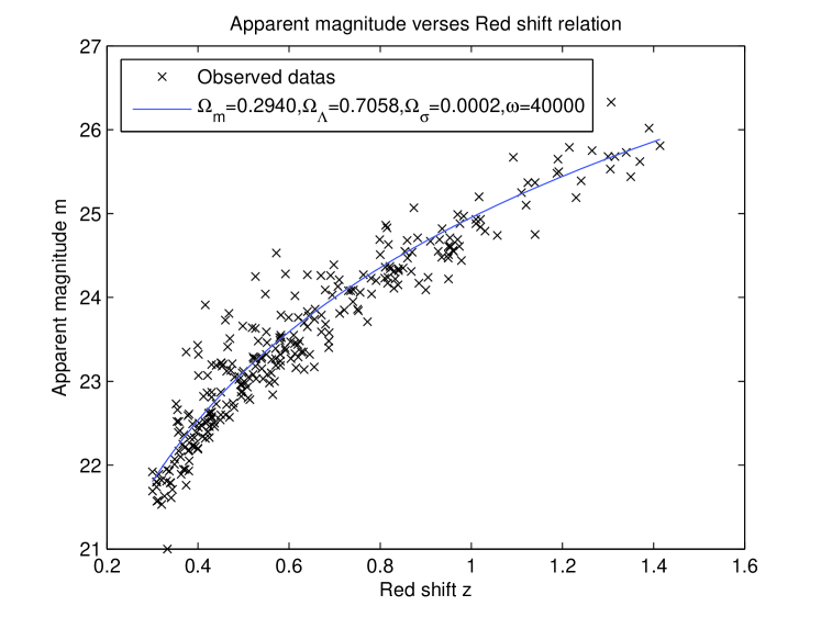
Figure 2: Apparent magnitude versus red shift best fit curve

5.5 ESTIMATION OF PRESENT VALUES OF HUBBLE’S CONSTANT $H_{0}$

We present a data set of the observed values of the Hubble parameters H(z) versus the red shift z with possible error in the form of following Table-1. These data points were obtained by various researchers from time to time, by using differential age approach.

Table 1: Hublle’s constant Table

$z$	$H(z)$	$\sigma_{H}$	Reference	Method
0.07	69	19.6	Moresco M. et al. [66]	DA
0.1	69	12	Zhang C. at el. [67]	DA
0.12	68.6	26.2	Moresco M. et al. [66]	DA
0.17	83	8	Zhang C. at el. [67]	DA
0.28	88.8	36.6	Moresco M. et al. [66]	DA
0.4	95	17	Zhang C. at el. [67]	DA
0.48	97	62	Zhang C. at el. [67]	DA
0.593	104	13	Moresco M. [68]	DA
0.781	105	12	Moresco M. [68]	DA
0.875	125	17	Moresco M. [68]	DA
0.88	90	40	Zhang C. at el. [67]	DA
0.9	117	23	Zhang C. at el. [67]	DA
1.037	154	20	Moresco M. [68]	DA
1.3	168	17	Zhang C. at el. [67]	DA
1.363	160	33.6	Moresco M., [68]	DA
1.43	177	18	Zhang C. at el. [67]	DA
1.53	140	14	Zhang C. at el. [67]	DA
1.75	202	40	Zhang C. at el. [67]	DA
1.965	186.5	50.4	Stern D at el. [69]	DA

In our model, Hubble’s constant H(z) versus red shift ’z’ relation Eq. (43) is reduced to

$$H^{2}=(0.9999)H_{0}^{2}[0.294(1+z)^{3}+0.0018(1+z)^{6}+0.7058]\,$$ (53)

Where we have taken $(\Omega_{m})_{0}=0.294$, $(\Omega_{\Lambda})_{0}=0.7058$, $\Omega_{\sigma}$ = 0.0002 and the coupling constant $\omega$ = $40000$. The Hubble Space Telescope (HST) observations of Cepheid variables [70] provides present value of Hubble’s constant $H_{0}$ in the range $H_{0}=73.8\pm 2.4km/s/Mpc$ . A large number of data sets of theoretical values of Hubble’s constant H(z) versus z, corresponding to $H_{0}$ in the range ($69\leq H_{0}\leq 74$ ) are obtained by using equation (53). It should be noted that the red shift $z$ are taken from Table-1 and each data set will consist of $19$ data points.

In order to get the best fit theoretical data set of Hubble’s constant $H(z)$ versus $z$, we calculate $\chi^{2}$ by using following statistical formula.

$$\chi_{SN}^{2}=\frac{X}{19},$$ (54)

where

$$X=\overset{19}{\underset{i=1}{\sum}}\frac{\left[\left(H\right)_{ob}-\left(H\right)_{th}\right]^{2}}{\sigma_{i}^{2}}.$$ (55)

Here the sums are taken over data sets of observed and theoretical values of Hubble’s constants. The observed values are taken from Table-1 and theoretical values are calculated from Eq. (49).

Using Eqs. (54)-(55), we have found that best fit value of Hubble’s constant $H_{0}$ is $71.9$ for minimum $\chi^{2}=0.5865$ Figure $3$ shows the dependence of Hubble’s constant with red shift. Hubble’s observed data points are closed to the graph corresponding to $(\Omega_{\Lambda})_{0}$ = $0.7058$, $(\Omega_{m})_{0}=0.294$ and $(\Omega_{\sigma})_{0}=0.0002$. This validates the proximity of observed and theoretical values.

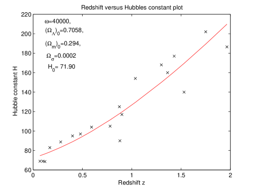
Figure 3: Variation of Hubble’s constant over red shift; Best fit curve

6 CERTAIN PHYSICAL PROPERTIES OF THE UNIVERSE

6.1 MATTER, DARK AND ANISOTROPIC ENERGY DENSITIES

The matter and dark energy densities of the universe are related to the energy parameters through following equation

$$\Omega_{m}=\frac{(\rho)_{m}}{\rho_{c}},~{}~{}\Omega_{\Lambda}=\frac{\rho_{\Lambda}}{\rho_{c}},~{}~{}\Omega_{\sigma}=\frac{(\rho)_{\sigma}}{\rho_{c}},$$ (56)

where

$$\rho_{c}=\frac{3c^{2}H^{2}}{8\pi G}=\frac{3c^{2}\phi H^{2}}{8\pi}.$$ (57)

So,

$$(\rho_{m})_{0}=(\rho_{c})_{0}(\Omega_{m})_{0}=,\;(\rho_{\Lambda})_{0}=(\rho_{c})_{0}(\Omega_{\Lambda})_{0}.$$ (58)

Now the present valu of $\rho_{c}$ is obtained as

$$(\rho_{c})_{0}=\frac{3c^{2}H_{0}^{2}}{8\pi G}=1.88\;h^{2}_{0}\times 10^{-29}\;gm/cm^{3}.$$

The estimated value of $h_{0}=0.719$. Therefore, the present value of matter and dark energy densities are given by

$$(\rho_{m})_{0}=0.5527h^{2}_{0}\times 10^{-29}gm/cm^{3},$$ (59)

$$(\rho_{\Lambda})_{0}=\rho_{c}(\Omega_{\Lambda})_{0}=1.3269h^{2}_{0}\times 10^{-29}gm/cm^{3},$$ (60)

and

$$(\rho_{\sigma})_{0}=0.0003h^{2}_{0}\times 10^{-29}gm/cm^{3}.$$ (61)

Here, we have taken

$$(\Omega_{m})_{0}=0.294\;(\Omega_{\Lambda})_{0}=0.7058\;\&\;(\Omega_{\sigma})_{0}=0.0002.$$

General expressions for matter and dark energies are given by

$$\rho=(\rho)_{0}\left(\dfrac{a_{0}}{a}\right)^{3}=(\rho)_{0}\left(1+z\right)^{3},$$ (62)

$$(\rho_{\Lambda})=\rho_{c}\;\Omega_{\Lambda},$$ (63)

and

$$(\rho_{\sigma})=(\rho_{\sigma})_{0}\left(\dfrac{a_{0}}{a}\right)^{6}=(\rho)_{0}\left(1+z\right)^{6}.$$ (64)

From above, we observe that the current matter and dark energy densities are very close to the values predicted by the various surveys described in the introduction.

6.2 AGE OF THE UNIVERSE

By using the standard formula

$$t=\intop_{0}^{t}dt=\intop_{0}^{A}\frac{dA}{AH},$$

we obtain the values of $t$ in terms of scale factor and redshift respectively

$$t=\intop_{0}^{A}\frac{\sqrt{1+\frac{5\omega+6}{6(\omega+1)^{2}}}dA}{AH_{0}\sqrt{(\Omega_{m})_{0}(\frac{A_{0}}{A})^{\frac{3\omega+4}{\omega+1}}+(\Omega_{\sigma})_{0}(\frac{A_{0}}{A})^{\frac{2(3\omega+4)}{\omega+1}}+(\Omega_{\Lambda})_{0}}}$$ (65)

$$t=\intop_{0}^{z}\frac{\sqrt{1+\frac{5\omega+6}{6(\omega+1)^{2}}}dz}{(1+z)H_{0}\sqrt{(\Omega_{m})_{0}(1+z)^{\frac{3\omega+4}{\omega+1}}+(\Omega_{\sigma})_{0}(1+z)^{\frac{2(3\omega+4)}{\omega+1}}+(\Omega_{\Lambda})_{0}}}$$ (66)

For $\omega=40000$, $(\Omega_{\Lambda})_{0}$ = $0.7058$, $(\Omega_{m})_{0}=0.294$ and $(\Omega_{\sigma})_{0}=0.0002$, Eq.(66) gives $t_{0}\rightarrow 0.9677H_{0}^{-1}$ for high redshift. This means that the present age of the universe is $t_{0}$ = $13.1392$ Gyrs as per our model. From WMAP data, the empirical value of present age of universe is $13.73_{-.17}^{+.13}Gyrs$ which is closed to present age of universe, estimated by us in this paper.

Figures $4$ shows the variation of time over red shift. At $z=0.8902$ curve becomes stationary. This provides present age of the universe This also indicated the consistency with recent observations.

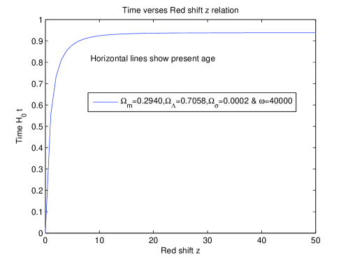
Figure 4: Variation of red shift over time and age of the universe

6.3 DECELERATION PARAMETER

From Eqs. (28), (32) and (34), we obtain the expressions for DP as

$$q=\frac{\omega+2}{2(\omega+1)}-\frac{3(\omega+1)}{2\omega+3}\;(\Omega_{\Lambda}-\Omega_{\sigma}).$$ (67)

Using Eqs. (26), (34), (42) and (43) in Eq. (67), we get following expression for deceleration parameter

$$q=\frac{\omega+2}{2(\omega+1)}-\frac{3(\omega+1)}{2\omega+3}\;\frac{\left(1+\frac{5\omega+6}{6(\omega+1)^{2}}\right)\left[\left(\Omega_{\Lambda}\right)_{0}-\left(\Omega_{\sigma}\right)_{0}(\frac{A_{0}}{A})^{6+\frac{2}{(\omega+1)}}\right]}{\left((\Omega_{m})_{0}\left(\frac{A_{0}}{A}\right)^{\frac{3\omega+4}{\omega+1}}+(\Omega_{\sigma})_{0}\left(\frac{A_{0}}{A}\right)^{\frac{2(3\omega+4)}{\omega+1}}+(\Omega_{\Lambda})_{0}\right)}.$$ (68)

In term of redshift, $q$ is given by

$$q=\frac{\omega+2}{2(\omega+1)}-\frac{3(\omega+1)}{2\omega+3}\;\frac{\left(1+\frac{5\omega+6}{6(\omega+1)^{2}}\right)\left(\left(\Omega_{\Lambda}\right)_{0}-\left(\Omega_{\sigma}\right)_{0}(1+z)^{6+\frac{2}{(\omega+1)}}\right)}{\left((\Omega_{m})_{0}(1+z)^{\frac{3\omega+4}{\omega+1}}+(\Omega_{\sigma})_{0}(1+z)^{\frac{2(3\omega+4)}{\omega+1}}+(\Omega_{\Lambda})_{0}\right)}.$$ (69)

For $\omega=40000$, the decelerating parameter is obtained as

$$q=0.5-1.5\;\left[(\Omega_{\Lambda})_{0}-(\Omega_{\sigma})_{0}(1+z)^{6}\right]\frac{1}{\left((\Omega_{m})_{0}\left(1+z\right)^{3}+(\Omega_{\sigma})_{0}\left(1+z\right)^{6}+(\Omega_{\Lambda})_{0}\right)}$$ (70)

As the present phase ($z=0$) of the universe is accelerating $q\leq 0\;i.e.\;\frac{\ddot{a}}{a}\geq 0$ , so we must have

$$(\Omega_{\Lambda})_{0}\geq\dfrac{(2\omega+3)(\omega+2)}{6(\omega+1)^{2}}+(\Omega_{\sigma})_{0}.$$ (71)

For $\omega=40000$ and $(\Omega_{\sigma})_{0}=0.0002$ the minimum value of $(\Omega_{\Lambda})_{0}$ is given by $(\Omega_{\Lambda})_{0}\geq 0.3335$ which is consistent with the present observed value of $(\Omega_{\Lambda})_{0}=0.7058$.

Putting $z=0$ in Eq. (70), the present value of deceleration constant is obtained as

$$q_{0}=-0.5584\;.$$ (72)

The Eq. (70) also provides

$$z_{c}\cong 0.6805\;at\;q=0$$ (73)

Therefore, the universe attains to the accelerating phase when $z<z_{c}$.

Converting redshift into time from Eq. (73), the value of $z_{c}$ is reduced to

$$z_{c}=0.6805\thicksim 0.4442H^{-1}_{0}yrs\thicksim 6.0337\times 10^{9}yrs.$$ (74)

So, the acceleration must have begun in the past at $6.0337\times 10^{9}yrs$ before from present. The figure $6$ shows how deceleration parameter increases from negative to positive over red shift which means that in the past universe was decelerating and at a instant $z_{c}\cong 0.6749$, it became stationary there after it goes on accelerating.

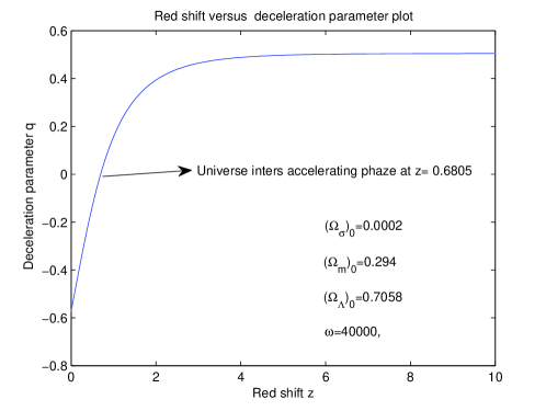
Figure 5: Variation of decelerating parameter over red shift. It represents accelerating universe at present.

6.4 SHEAR SCALAR

The shear scalar is given by

$$\sigma^{2}=\frac{1}{2}\sigma_{ij}\sigma^{ij},$$ (75)

where

$$\sigma_{ij}=u_{i;j}-\Theta(g_{ij}-u_{i}u_{j})$$ (76)

In our model

$$\sigma^{2}=\frac{\dot{d}^{2}}{d^{2}}=\frac{k^{2}}{\phi A^{6}}=(\Omega_{\sigma})_{0}H^{2}_{0}(1+z)^{\frac{2(3\omega+4)}{\omega+1}}$$ (77)

From Eq. (77), it is clear that shear scalar vanishes as $A\rightarrow\infty$.

6.5 RELATIVE ANISOTROPY

The relative anisotropy is given by

$$\frac{\sigma^{2}}{\rho_{m}}=\frac{3(\Omega_{\sigma})_{0}H^{2}_{0}(1+z)^{\frac{3\omega+5}{\omega+1}}}{(\rho_{c})_{0}(\Omega_{m})_{0}}$$ (78)

This follows the same pattern as shear scalar. This means that relative anisotropy decreases over scale factor i.e. time.

7 CONCLUSION

Table 2: Cosmological parameters at present

Cosmological Parameters	Values at Present
BD coupling constant $\omega$	40000
Dark energy parameter $(\Omega_{\Lambda})_{0}$	0.7058
Dust energy parameter $(\Omega_{m})_{0}$	0.294
Dust energy parameter $(\Omega_{\sigma})_{0}$	0.0002
Hubble’s constant $H_{0}$	71.90
Deceleration parameter $q_{0}$	$-0.5584$.
Dust energy density $(\rho_{m})_{0}$	$0.0.5527h_{0}^{2}\times 10^{-29}gm/cm^{3}$
Dark energy density $(\rho_{\Lambda})_{0}$	$1.3269h_{0}^{2}\times 10^{-29}gm/cm^{3}$
Anisotropic energy density $\rho_{\sigma})_{0}$	$0.0003h_{0}^{2}\times 10^{-29}gm/cm^{3}$
Age of the universe $t_{0}$	$13.1392~{}~{}Gyr$

We summarize our results by presenting Table-2 which displays the values of cosmological parameters at present obtained by us. We have found that the acceleration would have begun in the past at $6.0040\times 10^{9}yrs$ before from present. These results are in good agreements with the various surveys described in the introduction.

8 DISCLOSURE STATEMENT

The authors are not aware of any affiliation, membership, funding, or financial holding that might be perceived as affecting the objectivity of this paper.

References

• [1] S. Perlmutter et al. (Supernova Cosmology Project collaboration), Astrophys. J. 517, 565 (1999); [astro-ph/9812133].
• [2] A. G. Riess et al. (Spurnova Serach Team collaboration), Astron. J. 116, 1009 (1998); [arXiv:astro-ph/9805201].
• [3] D. N. Spergel et al. (WMAP collaboration), Astrophys. J. Suppl. 148, 175 (2003); [astro-ph/0302209].
• [4] M. Tegmark et al. (SDSS collaboration), Phys. Rev. D 69, 103501 (2004); [astro-ph/0310723].
• [5] P. A. R. Ade et al. (Planck Collaboration), A & A 594, A13 (2016); arXiv:1502.01589[astro-ph.Co].
• [6] R. K. Knop et al., Ap. J. 598, 102 (2003); [arXiv:astro-ph/0309368].
• [7] E. J. Copeland, M.Sami, and S. Tsujikawa, Int. J. Mod. Phys. D 15, 1753 (2006).
• [8] Ø. GrΓΈn and S. Hervik, Einstein’s general theory of relativity with modern applications in cosmology (Springer 2007).
• [9] K. Abazajian et al. (SDSS Collaboration), Astron. J. 128, 502 (2004).
• [10] V. Sahni and A. A.Starobinsky, Int. J. Mod. Phys. D 9, 373 (2000).
• [11] O. Heckmann and E. Schucking, Relativistic Cosmology In Gravitation: An Introduction to current research, ed L. Witten, Chap XI ( Willey, New York 1962) p. 438.
• [12] A. G. Doroshkevich and Ya. B. Zeldovich, Sov. Phys. JETP Lett. 5, 3 (1967).
• [13] C. W. Misner, Phys. Rev. Lett. 19, 533 (1967).
• [14] G. F. R. Ellis and M. A. H. MacCallum, Communi. Math. Phys. 12, 108 (1969).
• [15] R. A. Matzner, Astrophys. J. 157, 1085 (1969).
• [16] V. B. Johri and G. K. Goswami, Aust. J. Phys. 34, 261 (1981).
• [17] V. B. Johri and G. K. Goswami, Aust. J. Phys. 34, 235 (1983).
• [18] A. Pradhan and H. Amirhashchi, Mod. Phys. Lett. A 26, 2261 (2011); [arXiv:1110.1019[physics.gen-ph]].
• [19] A. Pradhan, Res. Astron. Astrophys. 13, 139 (2013); arXiv:1209.4826[physics.gen-ph].
• [20] A. Pradhan, A. K. Pandey, and R. K. Mishra, 88, 757 (2014).
• [21] A. Pradhan and B. Saha, Phys. Parti. Nuclei, 46, 310 (2015).
• [22] D. C. Maurya, R. Zia, and A. Pradhan, Int. J. Geom. Meth. Mod. Phys. 14, 1750077 (2017).
• [23] G. P. Singh, B. K. Bishi and P. K. Sahoo, Int. J. Geom. Meth. Mod. Phys. 13, 1650058 (2016).
• [24] P. K. Sahoo, P. Sahoo, and B. K. Bishi, Int. J. Geom. Meth. Mod. Phys. 14, 1750097 (2017).
• [25] C. L. Bennett et al., The Astrophys. J. Supplement 148, 1 (2003); [astro-ph/0302207].
• [26] G. K. Goswami, M. Mishra, and A. K. Yadav, Int. J. Theor. Phys. 54, 315 (2015).
• [27] G. K. Goswami, A. K. Yadav, R. N. Dewangan, and A. Pradhan, Astrophys. Space Sci. 361, 47 (2016).
• [28] G. K. Goswami, R. N. Dewangan, and A. K. Yadav, Astrophys. Space Sci. 361, 119 (2016).
• [29] G. K. Goswami, A. K. Yadav and R. N. Dewangan, Int. J. Theor. Phys. 55, 4651 (2016).
• [30] G. K. Goswami, R. N. Dewangan and A. K. Yadav, Gravitation & Cosmology 22, 388 (2016).
• [31] S. Weinberg, Gravitation and Cosmology: Principle and Application of the General Theory of Relativity (Wiley, NY 1972).
• [32] P. Jordan, Schwerkraft and Weltall (Friedrick Vieweg and Sohn, Braunschweig, 1955).
• [33] C. H. Brans and R. H. Dicke, Phys. Rev. A, Ser-2 124, 925 (1961).
• [34] R. H. Dicke, Phys. Rev. A, Ser-2 125, 2163 (1962).
• [35] J. V. Narlikar, An Introduction to Cosmology (Cambridge University Press 2002), p 483.
• [36] R. D. Reasenberg et al., Astrophys. J. 234, L219 (1979).
• [37] B. Bertotti et al., Nature 425, 374 (2003).
• [38] A. D. Felice et al., Phys. Rev. D 74, 103005 (2006).
• [39] V. Faraoni, Phy. Rev. D 70, 047301 (2004).
• [40] E. Elizalde, S. Nojiri, S. D. Odintsov, and Peng Wang, Phy. Rev. D 70, 103504 (2005).
• [41] S. Nojiri and S. D. Odintsov, Gen. Relativ. Gravit. 38, 1285 (2006).
• [42] A. Errahmani and T. Ouali, preprint (2008), arXiv:0706.0115[gr-qc].
• [43] W.-Q. Yang et al., Mod. Phys. Lett. 26, 191 (2011).
• [44] M. Sahraee and M. R. Setare, Int. J. Mod. Phys. D 25, 1650097 (2016).
• [45] B. K. Sahoo and L. P. Singh, Mod. Phys. Lett. 18, 2725 (2003).
• [46] M. Arik and M. C. Calik, Mod. Phys. Lett. 21, 1241 (2006).
• [47] El-Nabulsi A. Rami, Mod. Phys. Lett. 23, 401 (2008).
• [48] M. K. Mak and T. Harko, Int. J. Mod. Phys. D 12, 925 (2003).
• [49] E. Elizalde, S. Nojiri, and S. D. Odintsov, Phy. Rev. D 70, 043539 (2004) 043539.
• [50] S. Capozziello, R. De Ritis, C. Rubano, and P. Scudellaro, Int. J. Mod. Phys. D 05, 85 (1996).
• [51] S. Chakraborty, N. C. Chakraborty, and Ujjal Debnath, Mod. Phys. Lett. 18, 1549 (2003).
• [52] F. Rahaman and P. Ghosh, Mod. Phys. Lett. A 23, 2763 (2008).
• [53] S. Capozziello and G. Lambiase, Mod. Phys. Lett. 14, 2193 (1999).
• [54] A. Beesham, Mod. Phys. Lett. 13, 805 (1998).
• [55] S. Capozziello and G. Lambiase, Mod. Phys. Lett. 30, 1540032 (2015).
• [56] A. Chand, R. K. Mishra, and A. Pradhan, Astrophys. Space Sci. 361, 81 (2016).
• [57] O. Hrycyna and M. S. Lowski, Phys. Rev. D. 88, 064018 (2013).
• [58] Dieter Lorenz-Petzold, Phys. Rev. D. 29, 2399 (1984).
• [59] M. Sharif and S. Waheed, European Phys. Jour. C 72, 1876 (2012).
• [60] Y. Kucukakca et al., Gen. Relativ. Gravit. 44, 1893 (2012).
• [61] D. C. Maurya, R. Zia, and A. Pradhan, J. Experim. Theor. Phys. 123, 617 (2016).
• [62] G. K.Goswami, Res. Astron. Astrophys. 17, 1 (2017).
• [63] V. Petrosian, in M. S. Longair (ed.), Confrontation of cosmological theories with observational data, IAU Symp. 63, (D. Reidel Publ. Co., Dordrecht, 1974).
• [64] F. Occhionero and F. Vagnetti, Astron & Astrophys. 44, 329 (1975).
• [65] N. Suzuki et al., Astrophys. J. 746, 85 (2012).
• [66] M. Moresco et al., JCAP 1208, 006 (2012); [arXiv:1201.3609].
• [67] C. Zhang et al., Res. Astron. Astrophys. 14, 1221 (2014), [arXiv:1207.4541[astro-ph.CO]].
• [68] M. Moresco, Mon. Not. R. Astron. Soc. 450, L16 (2015).
• [69] D. Stern et al., JCAP 2010, 008 (2010).
• [70] V. Sahni, A. Shafieloo, and A. A. Starobinsky, Astrophys. J. Lett. 793 , L40 (2014).