Statefinder diagnostic for modified Chaplygin gas cosmology in $f(R,T)$ gravity with particle creation

Abstract In this paper, we have studied flat Friedmann–Lemaître–Robertson–Walker (FLRW) model with modified Chaplygin gas (MCG) having equation of state $p_{m}=A\rho-\frac{B}{\rho^{\gamma}}$, where $0\leq A\leq 1$, $0\leq\gamma\leq 1$ and $B$ is any positive constant in ${\footnotesize f(R,T)}$ gravity with particle creation. We have considered a simple parametrization of the Hubble parameter $H$ in order to solve the field equations and discussed the time evolution of different cosmological parameters for some obtained models showing unique behavior of scale factor. We have also discussed the statefinder diagnostic pair $\{r,s\}$ that characterizes the evolution of obtained models and explore their stability. The physical consequences of the models and their kinematic behaviors have also been scrutinized here in some detail.

Keywords ${\footnotesize f(R,T)}$ theory, Chaplygin gas, Particle creation, Parametrization
PACS number: 98.80 cq

1 Introduction

The current understanding of our observed Universe reveal that we live in an expanding Universe which is some $13.8$ billion years old that have been originated with a bang from a phase of very high density and temperature. Ever since this has been expanding. For a long time, it was assumed that either the expansion is gradually slow down caused by inward pull of gravity and would ultimately come to a halt after which Universe start to contract into a big crunch or the Universe expands eternally. However, it was at the end of twentieth century, the cosmological observations [1, 2] of type Ia supernovae revealed that the Universe might be expanding with an acceleration. The unexpected discovery surprised the cosmologists because the idea of cosmic acceleration was against the standard predictions of decelerating expansion caused by gravity. Later on it is predicted that the three quarters of the volume of Universe consists of some exotic stuff termed as “Dark energy” (DE) with highly negative pressure causing the acceleration. The subsequent discoveries in this direction gave more and more evidences for for a flat, dark energy dominated accelerating Universe. However, there are alternative way to explain the acceleration e.g. to modify the theory of gravity. In both the cases we confront new physics.

The Quantum field theory (QFT) and general theory of relativity (GTR) suggested the most viable candidate of DE - cosmological constant $\Lambda$ [3, 4, 5] introduced by Einstein. Though the model with a cosmological constant known as $\Lambda$CDM model is well versed it has some shortcomings [6]. Dynamical models of dark energy was proposed in the past few years with some effective candidates of DE [7, 8, 9, 10, 11, 12, 13, 14, 15, 16, 17, 18, 19, 20, 21] explaining some other observational features of the Universe. For a brief reviews on various dark energy models one can see [22, 23]. One of the most prospective candidate of DE is Chaplygin gas (CG) [24]. In order to understand the cosmic acceleration, Chaplygin gas is a simple characterization among the various class of dark energy models. The EoS of CG cosmological model is given by $p=-\frac{A}{\rho}$. Some of the inspiring and remarkable attributes of CG is that it can discuss the dark sector of the Universe with a single fluid component, leading to the unified models of DE and DM [25, 26, 27]. In the different eras of the Universe, CG plays a binary role: as in the early phase of the evolution of the Universe it acts like a dust matter and like a cosmological constant in the late time Universe [28]. CG exhibits an easy distorting of the standard $\Lambda$CDM model. One of the most prominent characteristic of CG cosmological model is that it provides a desirable phase transition from decelerated cosmic expansion to accelerated one. Some of the conceptual achievements of CG models has given in [29]. Further, CG has positive and bounded squared velocity of sound which is not obvious for its negative pressure fluids.

$$c_{s}^{2}=\frac{\partial p}{\partial\rho}=\frac{A}{\rho^{2}}\text{.}$$ (1)

Several generalization of CG has been proposed in the literature [30, 31, 32] due to its inspiring features. A generalized version of CG (GCG) is specified by its EoS, $p=-\frac{A}{\rho^{\gamma}}$, $0\leq\gamma\leq 1$, in which both DE and DM are just two different sides of a single exotic fluids. In accordance to have more consistency with observational data GCG was further extended to Modified Chaplygin gas (MCG) [33, 34, 35]. The MCG was presented with an EoS

$$p_{m}=A\rho-\frac{B}{\rho^{\gamma}},$$ (2)

where $0\leq A\leq 1$, $0\leq\gamma\leq 1$, and $B$ is any positive constant. MCG EoS consists of two parts, the first part recovers an ordinary perfect fluid with a linear barotropic EoS, and the second part connects pressure to some power of the inverse of energy density. In EoS of MCG, the case $B=0$ leads to standard perfect fluid while it reduces to the GCG EoS with $A=0$.

Matter creation in the Universe is also an important concept to be worth noting after the pioneering work of Parker [36, 37, 38, 39, 40]. The proposal was that it is the gravitational field acting on quantum vacuum responsible for the continuous creation of radiation and matter in an expanding Universe. Leonard Parker [41] suggested that the massless or massive particles production are not occurred in radiation or matter dominate eras [42, 43, 44, 45]. To understand the concept of this particle production there are two general approaches. The first one is the technique of adiabatic vacuum state [42, 43, 44, 45] and the second one is the technique of instantaneous Hamiltonian diagonalization [46, 47, 48, 49]. The particle creation scenario has many other aspects including the future deceleration phase in the Universe, existence of emergent Universe and chance of phantom Universe without the inclusion of phantom field. Also, to describe the current accelerating expansion of the Universe, a logical way can be the particle creation mechanism that based on QFT without the inclusion of any exotic component (DE) and the very concept was first proposed by Prigogine [50, 51].

In this paper, we have constructed some FLRW models with modified Chaplygin gas (MCG) EoS in $f(R,T)$ gravity with particle creation. Here, we have considered the simple parametrization of the Hubble parameter $H$ proposed in [52], to obtain some deterministic solutions to Einstein field equations (EFE). The physical behavior of energy density, matter pressure and the pressure due to particle creation are discussed for three different models. The paper is organized in seven sections as follows. Sect. 1 is of introductory nature. In sect. 2, the modification of GTR i.e., $f(R,T)$ gravity is discussed. In sect. 3, we have studied the field equations and solutions in which the energy density, matter pressure, and the pressure due to particle creation for three different models so obtained. In sect. 4, we have discussed a general probe for the expansion dynamics of the Universe using the statefinder diagnostic pair $\{r,s\}$. In sect. 5, we have discussed the stability criteria imposed on the velocity of sound $C_{s}^{2}$. Some distances in cosmology have been analyzed through kinematic tests in sect. 6 for all the models. Finally, the concluding remarks for the obtained models have been discussed in sect. 7.

2 ${\Large f(R,T)}$ gravity

The $f(R,T)$ theory is the modification of the general theory of relativity (GTR), where $R$ and $T$ are scalar curvature and the trace of stress energy-momentum tensor respectively [53]. The total gravitational action in $f(R,T)$ gravity is of the form

$$S=\frac{1}{16\pi G}\int\sqrt{-g}[f(R,T)+L_{m}]d^{4}x,$$ (3)

where $L_{m}$ is the matter Lagrangian density and $g$ the metric determinant. Taking the variation the action (2) into account w.r.t. the metric tensor components yields

$$G_{\mu\nu}+\left(g_{\mu\nu}\square-\nabla_{\mu}\nabla_{\nu}\right)=[8\pi+2f^{\prime}(T)]T_{\mu\nu}+2[f^{\prime}(T)p+\frac{1}{2}f(T)]g_{\mu\nu},$$ (4)

for which it is assumed that $f(R,T)=R+2f(T)$, where primes denote differentiation w.r.t. the argument. Now, we take $f(T)=\lambda T$ , with $\lambda$ a constant. This is the simplest non-trivial functional form of the function $f(R,T)$, which includes non-minimal matter-geometry coupling within $f(R,T)$ formalism. Moreover, it benefits from the fact that GR is retrieved when $\lambda=0$. Here, we consider perfect fluid as the matter source of the Universe and therefore, the energy-momentum tensor of matter Lagrangian can be taken as

$$T_{\mu\nu}=(\rho+p_{m})u_{\mu}u_{\nu}-p_{m}g_{\mu\nu},$$ (5)

where $\rho$ and $p_{m},$ are the dominant energy density and matter pressure of the cosmic fluid, respectively. $u^{\mu}=(0,0,0,1)$ is the components of the four velocity vector in the co-moving coordinate system which satisfies the conditions $u^{\mu}u_{\mu}=1$ and $u^{\mu}\nabla_{\nu}u_{\mu}=0$. We choose the perfect fluid matter as $L_{m}=-p_{m}$ in the action (2).

3 Field equations and solutions

The background metric satisfying the cosmological principle considered here in the form of the flat FLRW metric

$$ds^{2}=dt^{2}-a^{2}(t)\sum_{i=1}^{3}(dx_{i}^{2})\text{.}$$ (6)

We assume the matter content in the Universe filled with perfect fluid. In the presence of particle creation, the energy-momentum tensor of the perfect fluid (5) takes the form

$$T_{\mu\nu}=(\rho+p_{m}+p^{c})u_{\mu}u_{\nu}-(p_{m}+p^{c})g_{\mu\nu},$$ (7)

where $p^{c}$ is the pressure due to particle creation which depends on the particle production rate. The trace of the stress-energy-momentum in the influence of particle creation is

$$T=\rho-3(p_{m}+p^{c})\text{.}$$ (8)

The gravitational field equations in the above background are obtained as

$$3H^{2}=8\pi\rho+f(T)+2(\rho+p_{m}+p^{c})f^{\prime}(T),$$ (9)

$$2\dot{H}+3H^{2}=-8\pi(p_{m}+p^{c})+f(T).$$ (10)

Equations (8), (9) and (10) yield

$$3H^{2}=\left(8\pi+3\lambda\right)\rho-\lambda p_{m}-\lambda p^{c},$$ (11)

$$2\dot{H}+3H^{2}=\lambda\rho-\left(8\pi+3\lambda\right)p_{m}-\left(8\pi+3\lambda\right)p^{c}),$$ (12)

where an overhead dot indicates the derivative w.r.t. cosmic time $t$. Here, $p^{c}$ is the particle creation pressure which is a dynamic pressure that depends on production rate of particles. For, if $p^{c}$ is negative, this may compel the accelerating expansion of the Universe. Due to the firm constraints foist by local gravity measurements [54, 55, 56], the ordinary particle production is much limited and the radiation component has practically no influence on the acceleration. Some precise attention can be made to a process called adiabatic particle production which means, particles and also the entropy ($S$) are produced in a space-time but the entropy per particle $(\sigma=\frac{S}{N})$ (or specific entropy) is remains constant. For this case, the creation pressure reads [57, 58, 59]

$$p^{c}=-\frac{(\rho+p_{m})\Gamma}{3nH}\text{.}$$ (13)

To fulfil our goal, here in this paper, we use the parameterization of $\Gamma$ [60, 61, 62, 63, 64, 65, 66, 67, 68] as $\Gamma=3nH\eta$, which a source term indicating the production $(\Gamma>0)$ of particles and annihilation $(\Gamma<0)$ of the particles, $n$ refers to the particle number density and $H$ is the Hubble parameter (HP). The constant $\eta$ $\in[0,1]$. The term $n\eta>0$ can be denoted as a free parameter of the model that characterizes the particle production process. For, if $n\eta=0$ then, it means that there is no matter creation and for if high $n\eta$ then, there is high production of particle. But, in all of these cases, $\Gamma/3H\leq 1$. By use of $\Gamma=3nH\eta$ in (13), the particle creation pressure $p^{c}$ takes the form

$$p^{c}=-(\rho+p_{m})\eta\text{.}$$ (14)

Using equation (14) in equation (11) and (12), we obtain

$$3H^{2}=\left[8\pi+\left(3+\eta\right)\lambda\right]\rho+\lambda\left(\eta-1\right)p_{m},$$ (15)

$$2\dot{H}+3H^{2}=\left[8\pi\eta+\left(1+3\eta\right)\lambda\right]\rho+\left[8\pi\left(\eta-1\right)+3\lambda\left(\eta-1\right)\right]p_{m}\text{.}$$ (16)

Now, we have two field equations containing three variables $\rho,$ $p_{m}$, and $a$ in terms of $H$ and its derivative. We need to specify the matter content in the Universe which can be classified by its pressure. In the introduction, we have briefly discussed the importance of MCG in describing the late-time acceleration of the Universe having EoS (2) for which the field equations (15) and (16) reduce to

$$3H^{2}=\left[8\pi+\left(3+\eta\right)\lambda+A\left(\eta-1\right)\lambda\right]\rho-B\left(\eta-1\right)\lambda\rho^{-\gamma},$$ (17)

$$2\dot{H}+3H^{2} = \left[8\pi\eta+\left(1+3\eta\right)\lambda+8\pi A\left(\eta-1\right)+3A\left(\eta-1\right)\lambda\right]\rho$$ (18)

$$-\left[8\pi\left(\eta-1\right)B+3\left(\eta-1\right)\lambda B\right]\rho^{-\gamma}.$$

Eliminating $H^{2}$ from equation (17) and (18), we can write the field equations in a single evolution equation as

$$\dot{H}=\left(\eta-1\right)\left(1+A\right)\left(4\pi+\lambda\right)\rho-\left(\eta-1\right)\left(4\pi+\lambda\right)B\rho^{-\gamma},$$ (19)

which can alternatively be written as a polynomial equation in terms of $\rho$ given by

$$\rho^{\gamma+1}+\left[\frac{\dot{H}}{\left(1-\eta\right)\left(1+A\right)\left(4\pi+\lambda\right)}\right]\rho^{\gamma}-\frac{B}{\left(1+A\right)}=0\text{.}$$ (20)

Equation (20) can be solved for $\rho$ for a known scale factor $a(t)$ by providing particular values of $\gamma$. In literature, one can find number of parametrization of scale factor $a(t)$ and its higher order derivative terms i.e., first order derivative - Hubble parameter $H(t)$ and second order derivative - deceleration parameter $q(t)$. For a recent review on various parametrization, see [52]. The technique commonly known as the ‘model independent way’ to study dark energy models. Although the arbitrary constrain on any cosmological parameter seems to be an adhoc choice, this do not violate the background theory anyway for which the ‘model independent way’ or the ‘parametrization’ is a fiducial technique to study the models with an extra degree of freedom i.e., dark energy. Clearly, the dynamical behaviors of model depend on the functional form of assumed parameter. Following the same technique one can consider some specific parametrization of scale factor or its higher order derivatives for a comparative study. In this present work, we assume the simple and convenient form of Hubble parameter considered in [52] as

$$H(t)=\frac{\beta t^{k_{1}}}{\left(t^{k_{2}}+\alpha\right)^{k_{3}}},$$ (21)

where $\alpha,$ $\beta\neq 0,$ $k_{1},$ $k_{2},$ $k_{3}$ are real constants. $\alpha$, $\beta$ both may have the dimensions of time that can reduce to many known models under one umbrella by specifying $k_{1},$ $k_{2},$ $k_{3}$. However, we won’t consider all the models that have been discussed in [52]. Here, we consider only three models showing completely different evolution of scale factor e.g., the power law model [69] (that also leads to Berman’s model of constant deceleration parameter [70]), linearly varying deceleration parameter (LVDP) model [71] and a non singular model leading to a time varying deceleration parameter [72] for a comparative study with MCG equation of state and particle creation in $f(R,T)$ theory of gravity.

3.1 Model-I

For $k_{1}=-1,$ $k_{3}=0,$ $\forall$ $k_{2}$ in equation (21), we obtain the power law model with $H(t)=\frac{\beta}{t}$ and $a(t)=Ct^{\beta}$, where $\beta>0$ is dimensionless model parameter. The deceleration parameter $q=\frac{1}{\beta}-1\,$, which is constant throughout the evolution. Equation (20) reduces to

$$\rho^{\gamma+1}+\left[\frac{\beta}{\left(\eta-1\right)\left(1+A\right)\left(4\pi+\lambda\right)}\right]\frac{1}{t^{2}}\rho^{\gamma}-\frac{B}{1+A}=0,$$ (22)

which can not be solved for general $\gamma$. By providing some particular values of constants $A$, $B$, $\lambda$, $\eta$ and $\beta$, we show the evolution of energy density $\rho$ for different values of $\gamma$ which gives different evolution as can be seen from equation (2). Similarly, the evolution of pressure is shown in the plot below corresponding to the functional forms of $\rho$.

$\begin{array}[]{c@{\hspace{.1in}}cc}\includegraphics[width=158.99377pt]{rho-1.pdf}\hfil\hskip 7.22743pt&\includegraphics[width=158.99377pt]{pm-1.pdf}&\includegraphics[width=158.99377pt]{pc-1.pdf}\\ \mbox{(}a)\hfil\hskip 7.22743pt&\mbox{(}b)&\mbox{(}c)\end{array}$

Figure 1:  The plots of $\rho$, $p_{m}$ and $p_{c}$ Vs. time $t$ for the Model-I with $\mathit{A=}\frac{1}{3}$, $\mathit{B=1}$, $\lambda=1$, $\eta=0.25$ and $\beta=2$ for the particular values of $\gamma=0$, $0.5$, $1$.

From Fig. 1a, we can observe that the energy density $\rho$ is very very high ($\rightarrow\infty$) initially for all the three cases of $\gamma=0$, $0.5$, $1$. As the time unfolds, the energy density falls rapidly and attain a constant value in the late time Universe. In Fig. 1b, we see that the matter pressure decreases as time increases and remains negative which represents the accelerated cosmic expansion for all the three different values of $\gamma$. Fig. 1c depicts that the particle creation pressure $p_{c}$ is initially negative, overlying in all the three different values of $\gamma$ and tends to zero in the late-time. Here, we observe that the universe is accelerated expanding since $p^{c}$ is always negative, and the rate of particle production are initially high and later decreases to almost negligible corresponding to constant $\rho$.

3.2 Model-II

For $k_{1}=-1,$ $k_{2}=1,$ $k_{3}=1$ in equation (21), we have $H(t)=\frac{\beta}{t\left(t+\alpha\right)}$ and $a(t)=C\left(\frac{t}{t+\alpha}\right)^{\frac{\beta}{\alpha}}$, where $\alpha,\beta<0$ are model parameters, both have dimensions of time. The deceleration parameter $q(t)=-1+\frac{\alpha}{\beta}+\frac{2}{\beta}t$ vary linearly and shows phase transition from deceleration to acceleration in the near past. Equation (20) takes the form here as

$$\rho^{\gamma+1}+\left[\frac{\beta}{\left(\eta-1\right)\left(1+A\right)\left(4\pi+\lambda\right)}\right]\frac{2t+\alpha}{t\left(t+\alpha\right)^{2}}\rho^{\gamma}-\frac{B}{1+A}=0.$$ (23)

For some particular $\gamma$, equation (23) can be solved by providing suitable values to $A$, $B$, $\lambda\,$, $\eta$, $\alpha$ and $\beta$. The evolution of energy density $\rho$ and pressures are shown in the following figures.

$\begin{array}[]{c@{\hspace{.1in}}cc}\includegraphics[width=158.99377pt]{rho-2.pdf}\hfil\hskip 7.22743pt&\includegraphics[width=158.99377pt]{pm-2.pdf}&\includegraphics[width=158.99377pt]{pc-2.pdf}\\ \mbox{(}a)\hfil\hskip 7.22743pt&\mbox{(}b)&\mbox{(}c)\end{array}$

Figure 2: The plots of $\rho$, $p_{m}$ and $p_{c}$ Vs. time $t$ for the Model-II with $\mathit{A=}\frac{1}{3}$, $\mathit{B=1}$, $\lambda=1$, $\eta=0.25$ and $\alpha=-6$ & $\beta=-4$ for the particular values of $\gamma=0$, $0.5$, $1$.

In Fig. 2a, the plot of energy density $\rho$ starts with a very large value and after a short period of time it decreases promptly, remains constant for some time in the Universe, follows an immediate fall and subsequently diverges towards negative in future representing a future singularity at time $t=\alpha$. Fig. 2b depicts that the matter pressure $p_{m}$ recedes initially and gradually decreases with slow rate then after some time falls down rapidly and remains negative throughout the evolution of the Universe in all the three cases. In Fig. 2c, we observe that the particle creation pressure $p_{c}$ overlap for all the three different values of $\gamma$, initially negative and increases with time, tends to zero then expands with increasing rate and remains positive in the late time Universe. Here, we observe that the universe is accelerated expanding and the rate of particle production are initially high and later decreases to almost negligible, and again increases to attain high rate of particle production at $t=6$.

3.3 Model-III

For $k_{1}=1,$ $k_{2}=2,$ $k_{3}=1$ in equation (21), we obtain the non-singular bouncing model with $H(t)=\frac{\beta t}{t^{2}+\alpha}$ and $a(t)=C\left(t^{2}+\alpha\right)^{\frac{\beta}{2}}$, where $\alpha,\beta>0$ are model parameters. $\alpha$ has the dimension of square of time and $\beta$ is dimensionless. The deceleration parameter in this case comes out to be $q(t)=-1+\frac{1}{\beta}-\frac{\alpha}{\beta}\frac{1}{t^{2}}$. We have from equation (20),

$$\rho^{\gamma+1}+\left[\frac{\beta}{\left(1-\eta\right)\left(1+A\right)\left(4\pi+\lambda\right)}\right]\frac{\alpha-t^{2}}{\left(t^{2}+\alpha\right)^{2}}\rho^{\gamma}-\frac{B}{1+A}=0.$$ (24)

The evolution of energy density $\rho$ and pressures are shown in the following figures for different values of $\gamma$ and suitable choice of $A$, $B$, $\lambda\,$, $\eta$, $\alpha$ and $\beta$.

$\begin{array}[]{c@{\hspace{.1in}}cc}\includegraphics[width=158.99377pt]{rho-3.pdf}\hfil\hskip 7.22743pt&\includegraphics[width=158.99377pt]{pm-3.pdf}&\includegraphics[width=158.99377pt]{pc-3.pdf}\\ \mbox{(}a)\hfil\hskip 7.22743pt&\mbox{(}b)&\mbox{(}c)\end{array}$

Figure 3: The plots of $\rho$, $p_{m}$ and $p_{c}$ Vs. time $t$ for the Model-III with $\mathit{A=}\frac{1}{3}$, $\mathit{B=1}$, $\lambda=1$, $\eta=0.25$ and $\alpha=2$ & $\beta=\frac{1}{2}$ for the particular values of $\gamma=0$, $0.5$, $1$.

Fig. 3a illustrate that the energy density $\rho$ initiates with a finite value, increases promptly for a short period of time, attains its maximum then goes down and gradually decreases with slow rate and remains finite forever. In Fig. 3b, we see the matter pressure $p_{m}$ begins with a finite negative value, increases in a small interval of time but remains negative then drops again and start decreasing and eventually remains negative forever. Fig. 3c depicts that initially there is no matter creation, as time evolves particles get created and pressure $p_{c}$ starts decreasing promptly in a short span of time, then it raised up, expands as time derive, remains negative then tends to zero as $t\rightarrow\infty$. Here in this model, we observe that the universe is accelerated expanding since $p^{c}$ is negative. The rate of particle production are initially negligible, and again increases to attain high rate of particle production, and then gradually decreases at late time.

4 Statefinder diagnostics

In order to describe various dark energy models a method have been developed in [73] known as statefinder diagnostic. The statefinder diagnostic pair $\{r,s\}$ is a geometrical parameter that probe the expansion dynamics of the Universe through the higher derivatives of the scale factor $a$ i.e., Hubble parameter $H$ and the deceleration parameter $q$, and is defined by

$$r=\frac{\dddot{a}}{aH^{3}}\text{, \ \ }s=\frac{r-1}{3(q-\frac{1}{2})},$$ (25)

where $q\neq\frac{1}{2}$. For different dark energy models, the trajectories in the $s-r$ plane show diverge behavior. For example, in a spatially flat FRW Universe, the $\Lambda CDM$ model is identified as a fixed point $\{0,1\}$ in the $\{s,r\}$ diagram while the standard $SCDM$ model corresponds to a fixed point $\{1,1\}$ in the $\{s,r\}$ diagram. This analysis can successfully differentiate quintessence, Chaplygin gas, braneworld dark energy models and some other interacting dark energy models. For some particular model, the position of the fixed point $\{s,r\}$ can be calculated and located in the diagram. The statefinder diagnostics for different dark energy models have been discussed in references [75, 76, 77].

Here, we have obtained three different dark energy models that shows quite different evolution. We apply the statefinder diagnostic technique to calculate the diverging or converging behavior of our obtained dark energy models with respect to the $SCDM$ or $\Lambda CDM$ model. The $r,s$ parameters for our models-I are obtained as

$$r=1-\frac{3}{\beta}+\frac{2}{\beta^{2}},\text{ }s=\frac{2}{3\beta}.$$ (26)

Similarly, for model-II and model-III, the $\{r,s\}$ pair are obtained as

$$r = 1+\left(-\frac{3\alpha}{\beta}+\frac{2\alpha^{2}}{\beta^{2}}\right)+\left(-\frac{6}{\beta}+\frac{6\alpha}{\beta^{2}}\right)t+\frac{6}{\beta^{2}}t^{2},$$

$$s = \frac{2\alpha-\beta}{4\beta}+\frac{1}{\beta}t+\frac{4\alpha^{2}-9\beta^{2}}{12\beta(2\alpha-3\beta+4t)},$$ (27)

and

$$r = \frac{(3\alpha+(\beta-1)t^{2})(\beta-2)}{t^{2}\beta^{2}},$$

$$s = \frac{-6\alpha(\beta-2)+(6\beta-4)t^{2}}{6\alpha\beta+3\beta(3\beta-2)t^{2}},$$ (28)

respectively. We can see, in the power law model (model-I) $q$, $r$, $s$ are constants and has only one model parameter $\beta$. For different values of $\beta$, we have different expansion factors and can be analyzed in the following Table 1.

Table 1. $\beta$ $a(t)$ $H(t)$ $q$ $r$ $s$ $2$ $ct^{2}$ $\frac{2}{t}$ $-0.5$ $0$ $0.33$ $\frac{3}{2}$ $ct^{\frac{3}{2}}$ $\frac{3}{2t}$ $-0.33$ $-0.11$ $0.44$ $\frac{2}{3}$ $ct^{\frac{2}{3}}$ $\frac{2}{3t}$ $0.5$ $1$ $1$ $SCDM$ $\infty$ $ct$ $0$ $-1$ $1$ $0$ $\Lambda CDM$

In the model-II and the model-III, the parameters $q$, $r$, $s$ are time varying and contains two model parameters $\alpha$ and $\beta$. To have a better understanding of our model behavior, we plot the trajectories of the models in $s-r$ and $q-r$ planes.

$\begin{array}[]{c@{\hspace{0.1 in}}cc}\includegraphics[width=180.67499pt]{sr-1.pdf}\hfil\hskip 7.22743pt&\includegraphics[width=180.67499pt,height=173.44756pt]{qr-1.pdf}&\\ \mbox{(}a)\hfil\hskip 7.22743pt&\mbox{(}b)&\end{array}$

Figure 4:  The $\mathit{s-r}$ and $\mathit{q-r}$ diagrams in Model-I.

The left panel in Fig. 4 depicts the evolution of trajectory for different $\beta$ in $s-r$ plane. Initially the trajectory evolves and converges to the fixed point $SCDM$ ($s=1$, $r=1$). The value of both ‘$r$’ and ‘$s$’ start decline and attains their minimum value, after that both ‘$r$’ and ‘$s$’ increases towards the fixed point $\Lambda CDM$ ($s=0$, $r=1$). The horizontal line in the above diagram shows the progression of model from the $SCDM$ to $\Lambda CDM$ for increasing values of $\beta$. The right panel in Fig. 4 shows the evolution of trajectory in the $q-r$ plane. The trajectory in the $q-r$ plane behaves alike as in the $s-r$ plane but here in the $q-r$ plane, we can observe that the model converges to the steady state model $(SS)$ ($q=-1$, $r=1$) and transform from the fixed point $SCDM$ ($q=\frac{1}{2}$, $r=1$) to $\Lambda CDM$ and end up with the fixed point $SS$ with increasing values of $\beta$. A particular model for $\beta=2$ i.e., $a\sim t^{2}$ is shown in the figures.

$\begin{array}[]{c@{\hspace{.1in}}cc}\includegraphics[width=180.67499pt]{sr-2.pdf}\hfil\hskip 7.22743pt&\includegraphics[width=180.67499pt,height=173.44756pt]{qr-2.pdf}&\\ \mbox{(}a)\hfil\hskip 7.22743pt&\mbox{(}b)&\end{array}$

Figure 5:  The $\mathit{s-r}$ and $\mathit{q-r}$ diagrams in Model-II.

For model-II, the trajectories in the $s-r$ and $q-r$ planes are shown in Fig. 5. The left panel in Fig. 5 displays the evolution of trajectory with time in the $s-r$ diagram. The statefinder ($s-r$) is shown for two different values of model parameters $\alpha$ and $\beta$. The solid black trajectory does not begins with $SCDM$, evolves with time and touches the $\Lambda CDM$. A slightly change in the value of model parameters gives rise to a new trajectory (dashed line) which starts with $SCDM$, advanced with time and eventually coincident with the other curve and ultimately converges to $\Lambda CDM$. The right panel in Fig. 5 depicts the trajectories in $q-r$ plane for two different values of model parameters $\alpha$, $\beta$ which evolves with time. Both the trajectory initially start with the $SCDM$ but never touches to the $SS$ model.

$\begin{array}[]{c@{\hspace{.1in}}cc}\includegraphics[width=180.67499pt]{sr-3.pdf}\hfil\hskip 7.22743pt&\includegraphics[width=180.67499pt,height=166.2212pt]{qr-3.pdf}&\\ \mbox{(}a)\hfil\hskip 7.22743pt&\mbox{(}b)&\end{array}$

Figure 6:  The $\mathit{s-r}$ and $\mathit{q-r}$ diagrams in Model-III.

Finally, for model-III, the trajectories in the $s-r$ and $q-r$ planes are shown in Fig. 6. The left panel in Fig. 6 in the above figure displays the evolution of trajectory with time in the $s-r$ diagram. The statefinder ($s-r$) is shown for two different values of model parameters $\alpha$ and $\beta$. The solid black trajectory does not begins with $SCDM$, evolves with time and touches the $\Lambda CDM$. A change in the value of model parameters $\beta$ from $0.5$ to $3$ gives rise to a new trajectory (black dashed) which also deviates from $SCDM$ and intersect the point $\Lambda CDM$, plane for two different values of model parameters $\alpha$, $\beta$ which evolves with time. Both the trajectory deviates from $SCDM$ and $SS$ model.

5 Velocity of Sound and stability of model

As we know, the stability of linear perturbations is a critical test for the viability of any cosmological model which is beyond our scope here. However, a stringent constraint comes from imposing the Velocity of sound ($C_{s}^{2}$) to be sufficiently smaller than $1$ to avoid unwanted oscillations in the matter power spectrum. We plot $C_{s}^{2}$ for our obtained models with suitable choice of the parameters involved and are shown in the following figure:

$\begin{array}[]{c@{\hspace{.1in}}cc}\includegraphics[width=158.99377pt]{VC1.pdf}\hfil\hskip 7.22743pt&\includegraphics[width=158.99377pt]{VC2.pdf}&\includegraphics[width=158.99377pt]{VC3.pdf}\\ \mbox{(}a)\hfil\hskip 7.22743pt&\mbox{(}b)&\mbox{(}c)\end{array}$

Figure 7:  The plots of velocity of sound $C_{s}^{2}$ Vs. time $t$ in Model-I, II and III respectively for $\mathit{A=}$ $\frac{1}{3}$, $\mathit{B=1}$ and $\eta$ $\mathit{=0.25}$ for some selected value of $\gamma$.

Fig. 7 depicts the stability of our obtained models for the restricted values of the model parameters $\alpha$ and $\beta$ and the chosen particular values of other constants.

6 Some kinematic behavior

6.1 Lookback time

The lookback time $t_{L}$ to an object is the time elapsed between the detection of light today $(z=0)$ and at the time of emission of photons at a particular redshift $z$.

$$t_{L}=t_{0}-t(z)=\int_{a}^{a_{0}}\frac{dt}{\dot{a}},$$ (29)

where $a_{0}$ indicates the value of scale factor $a(t)$ at present time $t_{0}$, and by the relationship between the scale factor and redshift $z$

$$a_{0}=a(t)(1+z),\\$$ (30)

Here, for Model-I, II and III, the $t-z$ relation takes the form

$$t(z)=\beta H_{0}^{-1}(1+z)^{-\frac{1}{\beta}},$$ (31)

$$t(z)=\frac{\alpha}{(1+z)^{\frac{\alpha}{\beta}}\big{(}1+\frac{\alpha(\alpha+1)H_{0}}{\beta}\big{)}-1},$$ (32)

$$t(z)=\frac{\beta H_{0}^{-1}}{1+\alpha}\left[(1+z)^{\frac{-2}{\beta}}(1+\alpha)-\alpha\right]^{\frac{1}{2}},$$ (33)

where $H_{0}$ is the present day Hubble parameter of the Universe, $\alpha$ and $\beta$ are the model parameters.

6.2 Proper distance

The proper distance between two events is the distance between them in the frame of reference in which they occur at exactly same time and measured by a ruler at the time of observation. Proper distance is defined as $d(z)=a_{0}r$, where $r=r(z)$ is the radial distance of the object, which is given by

$$r(z)=\int_{t}^{t_{0}}\frac{dt}{a(t)},$$ (34)

For the above discussed Model I, II, III, the proper distance d(z) are given respectively:

$$d(z)=\frac{H_{0}^{-1}}{(\frac{1}{\beta}-1)}[1-(1+z)^{-(\frac{1}{\beta}-1)}],$$ (35)

$$d(z)=a_{0}\Big{[}\frac{\alpha t}{c(\alpha-\beta)}\big{(}\frac{t}{\alpha}\big{)}^{-\frac{\beta}{\alpha}}\times Hypergeometric\,2F1[-\frac{\beta}{\alpha},1-\frac{\beta}{\alpha},2-\frac{\beta}{\alpha},-\frac{t}{\alpha}]\Big{]}_{t}^{t_{0}},$$ (36)

$$d(z)=a_{0}\Big{[}\Big{(}\frac{t(t^{2}+\alpha)^{1-\frac{\beta}{2}}}{c\alpha}\Big{)}\times Hypergeometric\,2F1[1,\frac{3-\beta}{2},\frac{3}{2},-\frac{t^{2}}{\alpha}]\Big{]}_{t}^{t_{0}}.$$ (37)

Here, in order to make the plots, we have considered the series of the above mentioned Hypergeometric functions upto third order term.

$\begin{array}[]{c@{\hspace{.1in}}cc}\includegraphics[width=180.67499pt,height=144.54pt]{lookbck.pdf}\hfil\hskip 7.22743pt&\includegraphics[width=180.67499pt,height=144.54pt]{dz.pdf}&\\ \mbox{(}a)\hfil\hskip 7.22743pt&\mbox{(}b)&\end{array}$

Figure 8:  The plots of look back time $t_{L}$ and proper distance $d(z)$ Vs. redshift $z$ for the Model-I, II, III.

6.3 Luminosity distance

Luminosity distance $d_{l}$ of a source with redshift $z$ is defined by the relation

$$d_{l}^{2}=\frac{l}{4\pi L},$$ (38)

where $L$ is the flux measured and $l$ is the luminosity of the object. From equation (34) the luminosity distance is given by

$$d_{l}=(1+z)d(z).$$ (39)

6.4 Angular diameter distance

The angular diameter distance is defined by

$$d_{A}={\frac{l_{1}}{\theta}},$$ (40)

where $\displaystyle l_{1}$ is a physical size and $\displaystyle\theta$ is the angular size of an object, and the angular diameter distance $d_{A}$ of an object in terms of redshift $z$ is

$$d_{A}=\frac{d(z)}{1+z}=\frac{d_{l}}{(1+z)^{2}}.$$ (41)

$\begin{array}[]{c@{\hspace{.1in}}cc}\includegraphics[width=180.67499pt,height=144.54pt]{dl.pdf}\hfil\hskip 7.22743pt&\includegraphics[width=180.67499pt,height=144.54pt]{da.pdf}&\\ \mbox{(}a)\hfil\hskip 7.22743pt&\mbox{(}b)&\end{array}$

Figure 9:  The plots of luminosity distance $d_{l}$ and angular diameter distance $d_{A}$ Vs. redshift $z$ for the Model-I, II, III.

6.5 Deceleration parameter and phase transition

The deceleration parameter for model-I is constant throughout the evolution. For model-I, $q<0$ for $\beta>1$ and $q>0$ for $\beta<1$. Deceleration parameter for model-II and model-III is time varying and can be rewritten in terms of redshift $z$ using $t-z$ relationship (32) and (33) as $q(z)=-1+\frac{\alpha}{\beta}+\frac{2}{\beta}\frac{\alpha}{-1+(1+\alpha)(1+z)^{\frac{\alpha}{\beta}}}$ for model-II and $q(z)=-1+\frac{1}{\beta}-\frac{\alpha}{\beta}\frac{1}{-\alpha+(1+\alpha)(1+z)^{-\frac{2}{\beta}}}$ for model-III and can be analyzed in the following Table 2.

Table 2. redshift DP Value of DP, model-II Value of DP, model-III $z=\infty$ $q_{i}$ $-1+\frac{\alpha}{\beta}$ $-1+\frac{2}{\beta}$ $z=0$ $q_{0}$ $-1+\frac{2+\alpha}{\beta}$ $-1+\frac{1-\alpha}{\beta}$ $z=-1$ $q_{f}$ $-1-\frac{\alpha}{\beta}$ $-1+\frac{1}{\beta}$

Here $q_{i}$ is the initial value of DP at the time of big bang, $q_{0}$ being the present value of the DP and $q_{f}$ is the value of DP in the infinite future. The model parameters $\alpha$ and $\beta$ are to be chosen carefully so that we can have $q_{0}<0$ explaining the observation along with the positivity condition of the energy density $\rho$. For the appropriate values of $\alpha$ and $\beta$, model-II can exhibit a phase transition from deceleration to acceleration while model-III will show acceleration to deceleration phase transition or eternal acceleration. One can also constrain the values of $\alpha$ and $\beta$ through any observational data which will be defer to our future investigation. As the present observation strongly reveals a phase transition from deceleration to acceleration in the near past and our obtained model-II fits well in this context, we can plot a graph (see Fig. 10) showing the phase transition redshift ($z_{tr}$) and the present value of deceleration parameter ($q_{0}$).

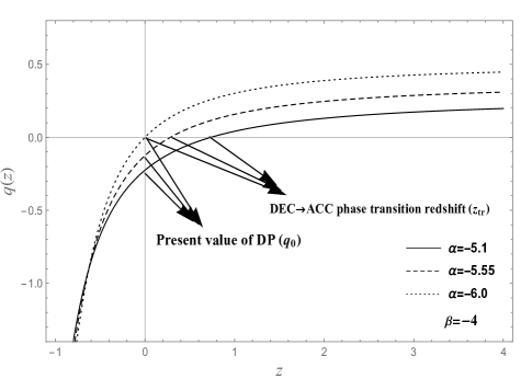
Figure 10:  The plot shows the deceleration to acceleration phase transition redshift ($z_{tr}$) and the present value of deceleration parameter ($q_{0}$) for model-II for fixed $\beta=-4.0$ and different $\alpha=-5.1,-5.55,-6.0$.

7 Discussion and Conclusion

In this paper, we explored the FLRW model with modified Chaplygin gas (MCG) in $f(R,T)$ gravity with particle creation. The deterministic solutions to Einstein field equations are obtained here by considering a simple parametrization of the Hubble parameter $H$ leading to diverge behavior of scale factor. We have examine the physical behavior of energy density, matter pressure, and the pressure due to particle creation for the obtained models.

• In case of Model-I, the Universe exhibits an initial singularity of the point-type at $t=0$. The model is well behaved in the range $0<t<\infty$ for the three cases of $\gamma$ = $0$, $0.5$ and $1$. It has been observed that the Universe starts with infinite dominant energy density $\rho$ at the initial singularity $t=0$, and monotonically decreases to attain a finite value at the late time. The matter pressure $p_{m}$ decreases and creation pressure $p^{c}$ increases as time increases and remains negative. Thus, the model shows accelerating expansion of the Universe for $\beta>1$ and the rate of particle production are high initially which gradually and stop at late times. The spatial volume increases exponentially with time which indicates that the Universe starts its expansion with zero volume and attains an infinite volume at late time.

• In case of Model-II, the Universe exhibits point type initial singularity $t=0$ and a future singularity of point-type at $t=\alpha$. The model is well behaved in the range $0<t<\alpha$ for the three cases of $\gamma$ = $0$, $0.5$ and $1$. It has been observed that the Universe starts with infinite dominant energy density $\rho$. As the time increases, the energy density decreases and diverges towards negative in future representing a future finite time singularity at $t=\alpha$. The matter pressure $p_{m}$ decreases and after some time it falls down rapidly and remains negative throughout the evolution of the Universe. Here, we observe that the Universe is expanding with acceleration at late times and the rate of particle production are initially high and later decreases to almost negligible, and again increases to attain high rate of particle production. The spatial volume increases with time which indicates that the Universe starts its expansion with zero volume and attains a finite volume at late time.

• In case of Model-III, the Universe is bouncing in nature and is free from initial singularity. It has been observed that the Universe starts with finite energy density which increases rapidly to its maximum value then gradually decreases to its smaller finite value. The matter pressure $p_{m}$ begins with a finite negative value remains negative forever. Here, this model starts with a finite acceleration and the rate of acceleration deceases with time. The rate of particle production are initially negligible, and again increases to attain high rate of particle production, and then gradually decreases at late time. The Universe starts its expansion with finite volume at $t=0$ and attains an infinite volume at late time. The model starts with infinite acceleration and decreases with time. The deceleration parameter takes finite positive value at late time. Here, the choice of the parameter $\beta$ is to be taken care for the positivity condition of energy density $\rho$ and explaining the present Universe.

• We have discussed the diverging behavior of different dark energy models-I, II and III using statefinder pair $\{r,s\}$. The model-I is a power law model in which $q$, $r$, $s$ are constants and depends on model parameter $\beta$ only. The model describes $\Lambda CDM$ and $SCDM$ when $\beta\rightarrow$ $\infty$ and $\beta=\frac{2}{3}$ respectively. Thus, the model-I describes for accelerating Universe when $\beta>1$ and we have different expansion factors for different values of $\beta$ (see Table-1).

• In the model-II, the parameters $q$, $r$, $s$ are time varying and contains two model parameters $\alpha$ and $\beta$. To analyze behaviors of our model better, we plot the trajectories of the models in $s-r$ and $q-r$ planes. Fig. 5a and Fig. 5b depict the evolution of trajectories with time in $s-r$ plane and $q-r$ plane respectively. Fig. 4a depicts the model converges from a fixed point $SCDM$ ($s=1$, $r=1$) to a fixed point $\Lambda CDM$ ($s=0$, $r=1$). Fig. 4b depicts the model converges to the steady state model (SS) ($q=-1$, $r=1$) and transform from the fixed point $SCDM$ ($q=\frac{1}{2}$, $r=1$) to $\Lambda CDM$ and end up with the fixed point $SS$.

• In the model-III, Fig. 6a displays the evolution of trajectory with time in the $s-r$ diagram. The statefinder ($s-r$) is shown for two different values of model parameters $\alpha$ and $\beta$. The solid black trajectory does not begins with $SCDM$ but passes through $\Lambda CDM$. The dashed line trajectory starts with $SCDM$ converges to $\Lambda CDM$. Fig. 6b depicts that both trajectories evolve with the $SCDM$ but never touches to the $SS$ model. Fig. 6a depicts that both trajectories do not start with $SCDM$ but both converge to $\Lambda CDM$ in $s-r$ plane. Fig. 6(b) depicts that neither both trajectories start with $SCDM$ nor both converge to $SS$.

• In Section 5, the stability condition $0\leq C_{s}^{2}\leq 1$ of the all the models-I, II, III for the three cases of $\gamma$ = $0$, $0.5$ and $1$ has been examined. The plots of Fig. 7a and Fig. 7c represent the model-I and III are perfectly stable for all $t$ but model-II is unstable due to Big-Rip singularity at $t=\alpha$. Thus, we conclude that models-I and III of the Universe completely stable and model-II is conditionally stable in $f(R,T)$ gravity with particle creation.

• In Section 6, we have studied the lookback time, proper distance, luminosity distance, angular diameter distance for our obtained models-I, II, III through the plots in Fig. 8, 9. We can see, the model-III behaves well in very small redshifts ($z<0.2$) while model-I and model-II show better behavior for higher redshifts also ($z>>1$).

• In subsection 6.5, we have discussed the phases of evolution of deceleration parameter. The DP is constant throughout the evolution for model-I while it is time varying for model-II and model-III. The model-III can exhibit phase transition from acceleration to deceleration or eternal acceleration while model-II can have deceleration to acceleration phase transition explaining the current observation. We can see, for ($\alpha=-6,\ \beta=-4$), the phase transition occurs at $z_{tr}=0$ and $q_{0}=0$ and the phase transition can be prepond by increasing $\alpha$ only i.e. for ($\alpha=-5.55,\ \beta=-4$), we have $z_{tr}=0.29$ & $q_{0}=-0.14$ and for ($\alpha=-5.1,\ \beta=-4$), we have $z_{tr}=0.72$ & $q_{0}=-0.23$.

Acknowledgements The authors express their thanks to CTP, Jamia Millia Islamia, New Delhi, India where a part of this work have been done and also thankful to Prof. M. Sami for a fruitful discussion to improve the paper. Author SKJP wishes to thank NBHM (DAE) for financial support through the post doctoral research fellowship.

References

- [1] A. G. Riess et al., Astron. J. 116, 1009 (1998)
- [2] S. Perlmutter et al., Astrophys. J. 517, 565 (1999)
- [3] P. J. E. Peebles et al., Rev. Mod. Phys. 432, 559 (2003)
- [4] V. Sahni et al., Int. J. Modern Phy. D 9, 373 (2000)
- [5] T. Padmanabhan, Phy. Rep. 380, 235 (2003)
- [6] S. Weinberg, Rev. Mod. Phys. 61, 1 (1989)
- [7] B. Ratra and P. J. E. Peebles, Phys. Rev. D 37, 3406 (1988)
- [8] R. R. Caldwell, R. Dave and P. J. Steinhardt, Phys. Rev. Lett. 80, 1582 (1998)
- [9] V. Sahni, M. Sami and T. Souradeep, Phys. Rev. D, 65 023518 (2002)
- [10] M. Sami and T. Padmanabhan, Phys. Rev. D 67 083509 (2003)
- [11] Armendariz-Picon, T. Damour and V. Mukhanov, Phys. Lett. B 458, 209 (1999)
- [12] T. Chiba, T. Okabe and M. Yamaguchi, Phys. Rev. D 62, 023511 (2000)
- [13] L. A. Boyle, R. R. Caldwell and M. Kamionkowski, Phys. Lett. B 545, 17 (2002)
- [14] A. Sen, Tachyon matter, J. High Energy Phys. 0207, 065 (2002)
- [15] T. Padmanabhan, Phys. Rev. D, 66, 021301 (2002)
- [16] B. Feng, X. L. Wang and X. M. Zhang, Phys. Lett. B 607, 35 (2005)
- [17] Z. K. Guo, Y. S. Pio, Y. Z. Zhang and X. M. Zhang, Phys. Lett. B 608, 177 (2005)
- [18] M. R. Setare, J. Sadeghi and A. R. Amani, Phys. Lett. B 660, 299 (2008)
- [19] M. R. Setare and E. N. Saridakis, Int. J. Mod. Phys. D 18, 549 (2009)
- [20] J. Khoury and A. Weltman, Phys. Rev. Lett. 93, 171104 (2004)
- [21] J. Khoury and A. Weltman, Phys. Rev. D 69, 044026 (2004)
- [22] E. J. Copeland, M. Sami and S. Tsujikawa, Int. J. Mod. Phys. D 15, 1753 (2006)
- [23] K. Bamba et al., Astrophys. Space Sci. 342 155 (2012)
- [24] S. Chaplygin, Sci. Mem. Moscow Univ. Math. Phys. 21, 1 (1904)
- [25] A. Y. Kamenshchik, U. Moschella and V. Pasquier, Phys. Lett. B 511, 265 (2001)
- [26] J. C. Fabris, S. V. B. Gonçalves and P. E. deS ouza, Gen. Rel. Grav. 34, 53 (2002)
- [27] M. C. Bento, O. Bertolami and A. A. Sen, Phys.Rev.D 66, 043507 (2002)
- [28] N. Bilic, G. B. Tupper and R. D. Viollier, Phys. Lett. B 535, 17 (2002)
- [29] V. Gorini, A. Yu. Kamenshchik and U. Moschella, Phys. Rev. D 67, 063509 (2003)
- [30] A. Dev, J. S. Alcaniz and D. Jain, Phys. Rev., D 67, 023515 (2003)
- [31] A. A. Sen and R. J. Scherrer, Phys. Rev., D 72, 063511 (2005)
- [32] U. Debnath, Chin. Phys. Lett. 28, 119801 (2011)
- [33] H. B. Benaoum, http://arxiv.org/abs/hep-th/0205140 (2002)
- [34] J. K. Singh and Sarita Rani, Appl. Math. and Comp., 259, 187 (2015)
- [35] J. K. Singh, N. K. Sharma and A. Beesham, Appl. Math. and Comp., 270, 567 (2015)
- [36] L. Parker, Phys. Rev. Lett., 21, 562 (1968)
- [37] S. A. Fulling, L. Parker, and B. L. Hu, Phys. Rev. D, 10, 3905 (1974)
- [38] L. Parker, Phys. Rev. D 17, 933 (1978)
- [39] N. J. Paspatamatiou, and L. Parker, Phys. Rev. D 19, 2283 (1979)
- [40] L. Parker, Fund. Cosm. Phys. 7, 201 (1982)
- [41] L. Parker, The creation of particles in an expanding universe, Ph.D. thesis, Harvard University, Cambridge, Massachusetts (1966)
- [42] L. Parker, Phys. Rev. 183, 1057 (1969)
- [43] L. Parker, Phys. Rev. Lett. 28, 705 (1972)
- [44] L. Parker, Phys. Rev. D 7, 976 (1973)
- [45] S. A. Fulling, Aspects of Quantum Field Theory in Curved Spacetime, Cambridge University Press, Cambridge (1989)
- [46] Yu. V. Pavlov, Grav. Cosmol. 14, 314 (2008)
- [47] A. A. Grib and S. G. Mamayev, Yad. Fiz. 10, 1276 (1969) [English transl.: Sov. J. Nucl. Phys. 10, 722 (1970)]
- [48] A. A. Grib, S. G. Mamayev and V. M. Mostepanenko, Gen. Rel. Grav. 7, 535 (1975)
- [49] A. A. Grib, S. G. Mamayev and V. M. Mostepanenko, Vaccum Quantum effects in Strong Fields, Friedmann Laboratory Publishing, St. Petesburg (1994)
- [50] I. Prigogine, J. Geheniau, E. Gunzig and P. Nardone, Proc. Nat. Acad. Sci. 85, 7428 (1988)
- [51] I. Prigogine, J. Geheniau , E. Gunzig and P. Nardone, Gen. Relativ. Grav. 21, 767 (1989)
- [52] S. K. J. Pacif, R. Myrzakulov and S. Myrzakul, Int. J. Geom. Meth. Mod. Phys. 14, 1750111 (2017)
- [53] T. Harko, F. S. N. Lobo, S. Nojiri, S. D. Odinstov, Phys. Rev. D 84, 024020 (2011)
- [54] J. Ellis, S. Kalara, K. A. Olive, C. Wetterich, Phys. Lett. B 228, 264 (1989)
- [55] P. J. E. Peebles and B. Ratra, Rev. Mod. Phys. 75, 559 (2003)
- [56] K. Hagiwara et al., Phys. Rev. D. 66, 010001 (2002)
- [57] M. O. Calvao, J. A. S. Lima, I. Waga, Phys. Lett. A 162, 223 (1992)
- [58] J. A. S. Lima, M. O. Calvao, I. Waga, Cosmology, Thermodynamics and Matter Creation, Frontier Physics, Essays in Honor of Jayme Tiomno, World Scientific, Singapore (1990)
- [59] J. A. S. Lima and A. S. M. Germano, Phys. Lett. A 170, 373 (1992)
- [60] R. C. Nunes and D. Pavon, Phys. Rev. D 91, 063526 (2015)
- [61] R. C. Nunes and S. Pan, Mon. Not. R. Astron. Soc. 459, 673 (2016)
- [62] S. Pan and S. Chakraborty, Adv. High Energy Phys. 2015, 654025 (2015)
- [63] S. Chakraborty, S. Pan, and S. Saha, Phys. Lett. B 738, 424 (2014)
- [64] S. Chakraborty, Phys. Lett. B 732, 81 (2014)
- [65] J. Dutta, S. Haldar, and S. Chakraborty, Astrophys. Space Sci. 361, 21 (2016)
- [66] S. Chakraborty and S. Saha, Phys. Rev. D 90, 123505 (2014)
- [67] J. de. Haro and S. Pan, Class. Quantum Grav. 33, 165007 (2016)
- [68] S. Pan, J. de. Haro, A. Paliathanasis and R. Jan. Slagter, Mon. Not. R. Astron. Soc. 460, 1445 (2016)
- [69] D. Lohiya and M. Sethi, Class. Quantum Grav., 16, 1545 (1999)
- [70] M. S. Berman, Phys. Rev. D 43, 1075 (1991)
- [71] O. Akarsu and T. Dereli, Int. J. Theoret. Phys., 51, 612 (2012)
- [72] Abdussattar and S. R. Prajapati, Astrophys. Space Sci., 331, 657 (2011)
- [73] V. Sahni, T. D. Saini, A. A. Starobinsky and U. Alam, JETP Lett. 77, 201 (2003)
- [74] U. alam et al., Mon. Not. Roy. Astron. Soc., 344, 1057 (2003)
- [75] M. Sami et al., Phys. Rev. D 86, (2012)
- [76] R. Myrzakulov and M. Shahalam, J. Cosm. Astroparticle Phys. 1310, 047 (2013)
- [77] S. Rani et al., J. Cosm. Astroparticle Phys. 1503, 031 (2015)