Higher order convergence rates for Bregman iterated variational regularization of inverse problems

Abstract

We study the convergence of variationally regularized solutions to linear ill-posed operator equations in Banach spaces as the noise in the right hand side tends to $0$. The rate of this convergence is determined by abstract smoothness conditions on the solution called source conditions. For non-quadratic data fidelity or penalty terms such source conditions are often formulated in the form of variational inequalities. Such variational source conditions (VSCs) as well as other formulations of such conditions in Banach spaces have the disadvantage of yielding only low-order convergence rates. A first step towards higher order VSCs has been taken by Grasmair (2013) who obtained convergence rates up to the saturation of Tikhonov regularization. For even higher order convergence rates, iterated versions of variational regularization have to be considered. In this paper we introduce VSCs of arbitrarily high order which lead to optimal convergence rates in Hilbert spaces. For Bregman iterated variational regularization in Banach spaces with general data fidelity and penalty terms, we derive convergence rates under third order VSC. These results are further discussed for entropy regularization with elliptic pseudodifferential operators where the VSCs are interpreted in terms of Besov spaces and the optimality of the rates can be demonstrated. Our theoretical results are confirmed in numerical experiments.

Keywords: inverse problems, variational regularization, convergence rates, entropy regularization, variational source conditions
MSC: 65J20, 65J22

1 Introduction

We consider linear, ill-posed inverse problems in the form of operator equations

$$Tf=g^{\mathrm{obs}}$$ (1)

with a bounded linear operator $T:\mathcal{X}\to\mathcal{Y}$ between Banach spaces $\mathcal{X}$ and $\mathcal{Y}$. We will assume that $T$ is injective, but that $T^{-1}:T(\mathcal{X})\to\mathcal{X}$ is not continuous. The exact solution will be denoted by $f^{\dagger}$, and the noisy observed data by $g^{\mathrm{obs}}\in\mathcal{Y}$, assuming the standard deterministic noise model

$$\|g^{\mathrm{obs}}-Tf^{\dagger}\|\leq\delta$$ (2)

with noise level $\delta>0$. To obtain a stable estimator of $f^{\dagger}$ from such data we will consider generalized Tikhonov regularization of the form

$$\hat{f}_{\alpha}\in\operatorname*{arg\,min}_{f\in\mathcal{X}}\left[\frac{1}{\alpha}\mathcal{S}(Tf-g^{\mathrm{obs}})+\mathcal{R}(f)\right] P_{1}$$ ()

with a convex, lower semi-continuous penalty functional $\mathcal{R}:\mathcal{X}\to\mathbb{R}\cup\{\infty\}$, $\mathbb{R}\not\equiv\infty$, a regularization parameter $\alpha>0$ and a data fidelity term

$$\mathcal{S}(g):=\tfrac{1}{q}\|g\|_{\mathcal{Y}}^{q}$$ (3)

for some $q>1$.

The aim of regularization theory is to bound the reconstruction error $\|\hat{f}_{\alpha}-f^{\dagger}\|$ in terms of the noise level $\delta$. Classically, in a Hilbert space setting, conditions implying such bounds have been formulated in terms of the spectral calculus of the operator $T^{*}T$,

$$f^{\dagger}\in(T^{*}T)^{\nu/2}(\mathcal{X})$$ (4)

for some $\nu>0$ and some initial guess $f_{0}$. In fact, using spectral theory it is easy to show that (4) yields

$$\left\|f^{\dagger}-\hat{f}_{\alpha}\right\|=\mathcal{O}\left(\delta^{\frac{\nu}{\nu+1}}\right)$$ (5)

for classical Tikhonov regularization (i.e. ($P_{1}$) with $\mathcal{R}(f)=\|f-f_{0}\|^{2}$ and $\mathcal{S}(g)=\|g\|_{\mathcal{Y}}^{2}$) if $\nu\in(0,2]$ and $\alpha\sim\delta^{\frac{2}{\nu+1}}$ (see e.g. [14]). The proof and even the formulation of the source condition (4) rely on spectral theory and have no straightforward generalizations to Banach space settings, and even in a Hilbert space setting the proof does not apply to frequently used nonquadratic functionals $\mathcal{R}$ and $\mathcal{S}$.

As an alternative, starting from [23], source conditions in the form of variational inequalities have been used:

$$\forall f\in\mathcal{X}\,:\,\left\langle f^{*},f^{\dagger}-f\right\rangle\leq\tfrac{1}{2}\Delta_{\mathcal{R}}^{f^{*}}(f,f^{\dagger})+\Phi\left(\mathcal{S}(Tf-Tf^{\dagger})\right)$$ (6)

Here $\Phi:[0,\infty)\to[0,\infty)$ is an index function (i.e. $\Phi$ is continuous and increasing with $\Phi(0)=0$), and $\Delta_{\mathcal{R}}^{f^{*}}$ denotes the Bregman distance (see Section 2 for a definition). Under the noise model (2) the variational source condition (6) implies the convergence rate $\Delta_{\mathcal{R}}^{f^{*}}(\hat{f}_{\alpha},f^{\dagger})\leq\mathcal{O}(\Phi(\delta^{2}))$, as shown in [20]. In contrast to spectral source conditions, the condition (6) is not only sufficient, but even necessary for this rate of convergence in most cases (see [26]). Moreover, due to the close connection to conditional stability estimates, variational source conditions can be verified even for interesting nonlinear inverse problems [25].

However, it is easy to see that (6) with quadratic $\mathcal{R}$ and $\mathcal{S}$ can only hold true for $\Phi$ satisfying $\lim_{\tau\to 0}\Phi(\tau)/\sqrt{\tau}>0$ (except for the very special case $f^{\dagger}\in\operatorname*{arg\,min}\mathcal{R}$), see [15, Prop. 12.10]. This implies that for quadratic Tikhonov regularization the condition (6) only covers spectral Hölder source condition (4) with indices $\nu\in(0,1]$. Several alternatives to the formulation (6) of the source condition suffer from the same limitation: multiplicative variational source conditions [2, 30], approximate source conditions [15], and approximate variational source conditions [15]. Symmetrized version of multiplicative variational source conditions (see [2, eq. (6)] and [1, §4]) cover a larger range of $\nu$, but have no obvious generalization to Banach space settings or non-quadratic $\mathcal{S}$ or $\mathcal{R}$. As shown in the first paper [23], the limiting case $\Phi(\tau)=c\sqrt{\tau}$ is equivalent to the source condition

$$\exists\overline{p}\in\mathcal{Y}^{*}\colon\qquad T^{*}\overline{p}=f^{*}$$ (7)

studied earlier in [5, 11]. To generalize also Hölder source conditions (4) with $\nu>1$ to the setting ($P_{1}$), Grasmair [21] imposed a variational source condition on $\overline{p}$, which turns out to be the solution of a Fenchel dual problem. Again the limiting case of this dual source condition, which we tag second order source condition, is equivalent to a simpler condition, $T\overline{\omega}\in\partial\mathcal{S}^{*}(\overline{p})$, which was studied earlier in [34, 36, 37]. Hence, Grasmair’s second order condition corresponds to the indices $\nu\in(1,2]$ in (4).

The aim of this paper is to derive rates of convergence corresponding to indices $\nu>2$, i.e. faster than $\|\hat{f}_{\alpha}-f^{\dagger}\|=\mathcal{O}(\delta^{2/3})$ in a Banach space setting. By the well-known saturation effect for Tikhonov regularization [22] such rates can occur in quadratic Tikhonov regularization only for $f^{\dagger}=0$. Therefore, we consider Bregman iterated Tikhonov regularization of the form

$$\hat{f}_{\alpha}^{(n)}\in\operatorname*{arg\,min}_{f\in\mathcal{X}}\left[\frac{1}{\alpha}\mathcal{S}(Tf-g^{\mathrm{obs}})+\Delta_{\mathcal{R}}\!\left(f,\hat{f}_{\alpha}^{(n-1)}\right)\right], P_{n}$$ ()

for $n\geq 2$, which reduces to iterated Tikhonov regularization if $\mathcal{R}(f)=\|f\|_{\mathcal{X}}^{2}$ and $\mathcal{S}(g)=\|g\|^{2}$. There is a considerable literature on this type of iteration from which we can only give a few references here. Note that for $\mathcal{R}(f)=\|f\|_{\mathcal{X}}^{2}$ the iteration ($P_{n}$) can be interpreted as the proximal point method for minimizing $\mathcal{T}(f):=\mathcal{S}(Tf-g^{\mathrm{obs}})$. In [6, 7, 10] generalizations of the proximal point method for general functions $\mathcal{T}$ on $\mathbb{R}^{d}$ were studied, in which the quadratic term is replaced by some Bregman distance (also called $D$-function). For $\mathcal{T}(f)=\mathcal{S}(Tf-g^{\mathrm{obs}})$ this leads to ($P_{n}$), and the references above discuss in particular the case entropy functions $\mathcal{R}$ considered below. In the context of total variation regularization of inverse problems, the iteration ($P_{n}$) was suggested in [35]. Low order convergence rates of this iterative method for quadratic data fidelity terms $\mathcal{S}$ and general penalty terms $\mathcal{R}$ were obtained in [4, 16, 17, 18]. We emphasize that in contrast to all the references above, we consider only small fixed number of iterations in ($P_{n}$) here to cope with the saturation effect. In particular, we study convergence in the limit $\alpha\to 0$, rather than $n\to\infty$.

The main contributions of this paper are:

• The formulation of variational source conditions of arbitrarily high order for quadratic regularization in Hilbert spaces (3.1) and the derivation of optimal convergence rates under these conditions (Theorem 3.2).

• Optimal convergence rates of general Bregman iterated variational regularization ($P_{n}$) in Banach spaces under a variational source condition of order $3$ (Theorem 4.5).

• Characterization of our new higher order variational source conditions in terms of Besov spaces for finitely smoothing operators, both for quadratic regularization (Corollary 5.3) and for maximum entropy regularization (Theorem 5.7).

The remainder of this paper is organized as follows: In the following section we review some basic properties of the Bregman iteration ($P_{n}$) and derive a general error bound. The following two sections §3 and §4 contain our main abstract convergence results in Hilbert and Banach spaces, respectively. The following section §5 is devoted to the interpretation of higher order variational source conditions. Our theoretical results are verified by numerical experiments for entropy regularization in §6, before we end the paper with some conclusions. Some results on duality mappings and consequences of the Xu-Roach inequality are collected in an appendix.

2 Bregman iterations

Let us first recall the definition of the Bregman distance for a convex functional $\mathcal{R}:\mathcal{X}\to(-\infty,\infty]$: Let $f_{0},f\in\mathcal{X}$ and assume that ${f_{0}}^{*}\in\mathcal{X}^{*}$ belongs to the subdifferential of $\mathcal{R}$ at $f_{0}$, $f_{0}^{*}\in\partial\mathcal{R}(f_{0})$ (see e.g. [12, §I.5]). Then we set

$$\Delta_{\mathcal{R}}^{f_{0}^{*}}(f,f_{0}):=\mathcal{R}(f)-\mathcal{R}(f_{0})-\left\langle f_{0}^{*},f-f_{0}\right\rangle.$$

In the context of inverse problems Bregman distances were introduced in [5, 11]. If there is no ambiguity, we sometimes omit the superindex $f_{0}^{*}$. This is in particular the case if $\mathcal{R}$ is Gateaux differentiable, implying that $\partial\mathcal{R}(f_{0})=\{\mathcal{R}^{\prime}[f_{0}]\}$. In the case $\mathcal{R}(f)=\|f\|_{\mathcal{X}}^{2}$ with a Hilbert space $\mathcal{X}$, the Bregman distance is simply given by $\Delta_{\mathcal{R}}(f,f_{0})=\|f-f_{0}\|_{\mathcal{X}}^{2}$. In general, however, the Bregman distance is neither symmetric nor does it satisfy a triangle inequality. Later we will also use symmetric Bregman distances $\Delta_{\mathcal{R}}^{\mathrm{sym},f_{1}^{*},f_{2}^{*}}(f_{1},f_{2}):=\Delta_{\mathcal{R}}^{f_{1}^{*}}(f_{2},f_{1})+\Delta_{\mathcal{R}}^{f_{2}^{*}}(f_{1},f_{2})$ for $f_{1},f_{2}\in\mathcal{X}$ and $f_{j}^{*}\in\partial\mathcal{R}(f_{j})$, which satisfy

$$\Delta_{\mathcal{R}}^{\rm{sym}}(f_{1},f_{2})=\left\langle f_{2}^{*}-f_{1}^{*},f_{2}-f_{1}\right\rangle.$$

Under the same assumptions the following identity follows from Young’s equality:

$$\Delta_{\mathcal{R}}^{f_{2}^{*}}(f_{1},f_{2})=\Delta_{\mathcal{R}^{*}}^{f_{1}}(f_{2}^{*},f_{1}^{*}).$$ (8)

Let us show that Bregman iterations ($P_{n}$) are well-defined for general data fidelity terms of the form (3). To this end we impose the following conditions:

Assumption 2.1.

Let $\mathcal{X},\mathcal{Y}$ be Banach spaces, and assume that $\mathcal{Y}$ is $q$-smooth and $r$-convex $1<q\leq 2\leq r<\infty$ (see Definition A.1). Moreover, consider an operator $T\in L(\mathcal{X},\mathcal{Y})$, a convex, proper, lower semi-continuous functional $\mathcal{R}:\mathcal{X}\to(-\infty,\infty]$ and $\mathcal{S}$ given by (3). Assume that the functional

$$f\mapsto\frac{1}{\alpha}\mathcal{S}(Tf-g^{\mathrm{obs}})+\Delta_{\mathcal{R}}^{f_{0}^{*}}(f,f_{0})$$

has a unique minimizer for all $(f_{0},f_{0}^{*})\in\mathcal{X}\times\mathcal{X}^{*}$ such that $f_{0}^{*}\in\partial\mathcal{R}(f_{0})$.

Existence and uniqueness of minimizers has been shown in many cases under different assumptions in the literature. As the main focus of this work are convergence rates, we just assume this property here. We just mention that it can be shown by a standard argument from calculus of variations under the additional assumptions that the sublevel sets $\{f\in\mathcal{X}\colon\Delta_{\mathcal{R}}^{f_{0}^{*}}(f,f_{0})\leq M\}$ are weakly or weakly^∗ sequentially compact for all $M\in\mathbb{R}$. For $\mathcal{R}$ given by the cross entropy functional discussed in §5.3 such weak continuity of sublevel sets in $L^{1}$ was shown in [11, Lemma 2.3]. For total variation regularization Assumption 2.1 has been shown in [35, Prop. 3.1].

For a number $s\in(1,\infty)$ we will denote by $s^{*}$ the conjugate number satisfying $\tfrac{1}{s}+\tfrac{1}{s^{*}}=1$. Recall that

$$\mathcal{S}^{*}(p)=\frac{1}{q^{*}}\left\|p\right\|_{\mathcal{Y}^{*}}^{q^{*}}$$

and that $\mathcal{S}(\cdot-g^{\mathrm{obs}})^{*}(p)=\mathcal{S}^{*}(p)+\langle p,g^{\mathrm{obs}}\rangle$. The initial step of the Bregman iteration is the Tikhonov minimization problem ($P_{1}$). The Fenchel dual to ($P_{1}$) is

$$\hat{p}_{\alpha}\in\operatorname*{arg\,min}_{p\in\mathcal{Y}^{*}}\left[\frac{1}{\alpha}\mathcal{S}^{*}(-\alpha p)-\langle p,g^{\mathrm{obs}}\rangle+\mathcal{R}^{*}(T^{*}p)\right]. P_{1}^{*}$$ ()

By Theorem 4.1 in [12, Chap. III], $\hat{p}_{\alpha}\in\mathcal{Y}^{*}$ exists as the functional $\mathcal{S}$ is continuous everywhere. As $\mathcal{Y}$ is $q$-smooth, $\mathcal{Y}^{*}$ is $q^{*}$-convex, and hence $\hat{p}_{\alpha}$ is unique. If $\hat{f}_{\alpha}$ exists as well we have strong duality for ($P_{1}$),($P_{1}^{*}$), and by [12, Chap. III, Prop. 4.1] the following extremal relations hold true:

$$T^{*}\hat{p}_{\alpha}\in\partial\mathcal{R}(\hat{f}_{\alpha})\quad\text{ and }\quad-\alpha\hat{p}_{\alpha}\in\partial\mathcal{S}(T\hat{f}_{\alpha}-g^{\mathrm{obs}}).$$ (9)

Using the Bregman distance $\mathcal{R}_{2}(f):=\Delta_{\mathcal{R}}^{T^{*}\hat{p}_{\alpha}}(f,\hat{f}_{\alpha})$ we can give a precise definition of the second step of the Bregman iteration ($P_{n}$):

$$\hat{f}_{\alpha}^{(2)}\in\operatorname*{arg\,min}_{f\in\mathcal{X}}\left[\frac{1}{\alpha}\mathcal{S}(Tf-g^{\mathrm{obs}})+\mathcal{R}_{2}(f)\right]. P_{2}$$ ()

Like this we can recursively prove well-definedness of the Bregman iteration ($P_{n}$) as follows:

Proposition 2.2.

Suppose Assumption 2.1 holds true. Let $\hat{f}_{\alpha}^{(1)}:=\hat{f}_{\alpha}$ be the solution to $(P_{1}):=\eqref{eq:genTikh}$, and set $\mathcal{R}_{1}:=\mathcal{R}$. Then for $n=1,2,\dots$ the dual solutions

$$\hat{p}_{\alpha}^{(n)}\in\operatorname*{arg\,min}_{p\in\mathcal{Y}^{*}}\left[\frac{1}{\alpha}\mathcal{S}^{*}(-\alpha p)-\langle p,g^{\mathrm{obs}}\rangle+\mathcal{R}_{n}^{*}(T^{*}p)\right] P_{n}^{*}$$ ()

are well defined, and we have strong duality between $(P_{n})$ and $(P_{n}^{*})$. Moreover,

$$f_{n}^{*}:=\sum_{k=1}^{n}T^{*}\hat{p}_{\alpha}^{(k)}\in\partial\mathcal{R}\left(\hat{f}_{\alpha}^{(n)}\right),$$

such that we can define $\mathcal{R}_{n+1}(f):=\Delta_{\mathcal{R}}^{f_{n}^{*}}(f,\hat{f}_{\alpha}^{(n)})$ as well as

$$\hat{f}_{\alpha}^{(n+1)}\in\operatorname*{arg\,min}_{f\in\mathcal{X}}\left[\frac{1}{\alpha}\mathcal{S}(Tf-g^{\mathrm{obs}})+\mathcal{R}_{n+1}(f)\right]. P_{n+1}$$ ()

Proof.

We need to prove the existence of $\hat{p}_{\alpha}^{(n)}$ as well as the fact that the subdifferential $\partial\mathcal{R}(\hat{f}_{\alpha}^{(n)})$ contains $\sum_{k=1}^{n}T^{*}\hat{p}_{\alpha}^{(k)}$ . The existence of $\hat{p}_{\alpha}^{(n)}$ as well as strong duality for $(P_{n}),(P_{n}^{*})$ follows once again from Theorem 4.1 in [12]. The second statement can be proved by induction. The base case was shown in (9). By strong duality we have

$$T^{*}\hat{p}_{\alpha}^{(n)}\in\partial\mathcal{R}_{n}(\hat{f}_{\alpha}^{(n)})=\partial\mathcal{R}(\hat{f}_{\alpha}^{(n)})-\sum_{k=1}^{n-1}T^{*}\hat{p}_{\alpha}^{(k)}.$$

Therefore, we have $\sum_{k=1}^{n}T^{*}\hat{p}_{\alpha}^{(k)}\in\partial\mathcal{R}(\hat{f}_{\alpha}^{(n)})$ and can define $\mathcal{R}_{n+1}$ in the way we claimed.

A useful fact about the penalty functionals $\mathcal{R}_{n}$ is that their corresponding Bregman distances coincide for all $n\in\mathbb{N}$ as they only differ by an affine linear functional:

Lemma 2.3.

Let $f_{0}\in\mathcal{X},f_{0}^{*}\in\partial\mathcal{R}(f_{0})$ and $\tilde{p}:=\sum_{k=1}^{n-1}\hat{p}_{\alpha}^{(k)}$. Then we have

$$\Delta_{\mathcal{R}_{n}}^{f_{0}^{*}-T^{*}\tilde{p}}(f,f_{0})=\Delta_{\mathcal{R}}^{f_{0}^{*}}(f,f_{0}).$$

Proof.

By Proposition 2.2 we have $T^{*}\tilde{p}\in\partial\mathcal{R}(\hat{f}_{\alpha}^{(n-1)})$ so $f_{0}^{*}-T^{*}\tilde{p}\in\partial\mathcal{R}_{n}(f_{0})$ and

$$\Delta_{\mathcal{R}_{n}}^{f_{0}^{*}-T^{*}\tilde{p}}(f,f_{0}) =\Delta_{\mathcal{R}}^{T^{*}\tilde{p}}(f,\hat{f}_{\alpha}^{(n-1)})-\Delta_{\mathcal{R}}^{T^{*}\tilde{p}}(f_{0},\hat{f}_{\alpha}^{(n-1)})-\left\langle f_{0}^{*}-T^{*}\tilde{p},f-f_{0}\right\rangle$$

$$=\mathcal{R}(f)-\mathcal{R}(f_{0})-\left\langle f_{0}^{*},f-f_{0}\right\rangle=\Delta_{\mathcal{R}}^{f_{0}^{*}}(f,f_{0}).$$

The following lemma describes the first step towards our bounds on the error in the Bregman distance. All that is then left is to construct appropriate vectors $f$ which approximately minimize the functional on the right hand side.

Lemma 2.4.

Suppose Assumption 2.1 holds true and there exists $\overline{p}\in\mathcal{Y}^{*}$ such that $T^{*}\overline{p}\in\partial\mathcal{R}(f^{\dagger})$. With the notation of Proposition 2.2 define $s^{(n)}_{\alpha}:=\overline{p}-\sum_{k=1}^{n-1}\hat{p}_{\alpha}^{(k)}$. Then

$$\Delta_{\mathcal{R}}^{T^{*}\overline{p}}\left(\hat{f}_{\alpha}^{(n)},f^{\dagger}\right)\leq\inf_{f\in\mathcal{X}}\bigg{[}\frac{1}{\alpha}\mathcal{S}\left(Tf-g^{\mathrm{obs}}\right)+\left\langle s^{(n)}_{\alpha},Tf-g^{\mathrm{obs}}\right\rangle$$

$$+\frac{1}{\alpha}\mathcal{S}^{*}\left(-\alpha s^{(n)}_{\alpha}\right)+\Delta_{\mathcal{R}}^{T^{*}\overline{p}}\left(f,f^{\dagger}\right) \bigg{]}.$$

Proof.

Due to the minimizing property of $\hat{f}_{\alpha}^{(n)}$ we have

$$\frac{1}{\alpha}\mathcal{S}\left(T\hat{f}_{\alpha}^{(n)}-g^{\mathrm{obs}}\right)+\mathcal{R}_{n}\left(\hat{f}_{\alpha}^{(n)}\right)\leq\frac{1}{\alpha}\mathcal{S}\left(Tf-g^{\mathrm{obs}}\right)+\mathcal{R}_{n}(f),$$

for all $f\in\mathcal{X}$, which is equivalent to

$$\mathcal{R}_{n}\left(\hat{f}_{\alpha}^{(n)}\right)-\mathcal{R}_{n}(f)\leq\frac{1}{\alpha}\mathcal{S}\left(Tf-g^{\mathrm{obs}}\right)-\frac{1}{\alpha}\mathcal{S}\left(T\hat{f}_{\alpha}^{(n)}-g^{\mathrm{obs}}\right).$$ (10)

As $T^{*}s^{(n)}_{\alpha}=T^{*}\overline{p}-f^{*}_{n-1}\in\partial\mathcal{R}(f^{\dagger})-f^{*}_{n-1}=\partial\mathcal{R}_{n}(f^{\dagger})$ by Proposition 2.2, it follows that

$$\Delta_{\mathcal{R}_{n}}^{T^{*}s^{(n)}_{\alpha}}\left(\hat{f}_{\alpha}^{(n)},f^{\dagger}\right) =\mathcal{R}_{n}\left(\hat{f}_{\alpha}^{(n)}\right)-\mathcal{R}_{n}\left(f^{\dagger}\right)-\left\langle T^{*}s^{(n)}_{\alpha},\hat{f}_{\alpha}^{(n)}-f^{\dagger}\right\rangle$$

$$\leq\frac{1}{\alpha}\mathcal{S}(Tf-g^{\mathrm{obs}})-\frac{1}{\alpha}\mathcal{S}\left(T\hat{f}_{\alpha}^{(n)}-g^{\mathrm{obs}}\right)$$

$$\quad-\left\langle T^{*}s^{(n)}_{\alpha},\hat{f}_{\alpha}^{(n)}-f^{\dagger}\right\rangle+\mathcal{R}_{n}(f)-\mathcal{R}_{n}\left(f^{\dagger}\right).$$

Due to the strong duality (Propostion 2.2) the extremal relation $-\alpha\hat{p}_{\alpha}^{(n)}\in\partial\mathcal{S}(T\hat{f}_{\alpha}^{(n)}-g^{\mathrm{obs}})$ holds true, and thus the generalized Young equality yields

$$-\frac{1}{\alpha}\mathcal{S}\left(T\hat{f}_{\alpha}^{(n)}-g^{\mathrm{obs}}\right) =\frac{1}{\alpha}\mathcal{S}^{*}\left(-\alpha\hat{p}_{\alpha}^{(n)}\right)+\left\langle\hat{p}_{\alpha}^{(n)},T\hat{f}_{\alpha}^{(n)}-g^{\mathrm{obs}}\right\rangle$$

$$=\frac{1}{\alpha}\mathcal{S}^{*}\left(-\alpha s^{(n)}_{\alpha}\right)+\left\langle s^{(n)}_{\alpha},T\hat{f}_{\alpha}^{(n)}-g^{\mathrm{obs}}\right\rangle$$

$$\quad-\frac{1}{\alpha}\Delta_{\mathcal{S}^{*}}\left(-\alpha s^{(n)}_{\alpha},-\alpha\hat{p}_{\alpha}^{(n)}\right)$$

$$\leq\frac{1}{\alpha}\mathcal{S}^{*}\left(-\alpha s^{(n)}_{\alpha}\right)+\left\langle s^{(n)}_{\alpha},T\hat{f}_{\alpha}^{(n)}-g^{\mathrm{obs}}\right\rangle$$

where we have used that the Bregman distance is non-negative. Combining this gives

$$\Delta_{\mathcal{R}_{n}}^{T^{*}s^{(n)}_{\alpha}}\left(\hat{f}_{\alpha}^{(n)},f^{\dagger}\right) \leq\frac{1}{\alpha}\mathcal{S}(Tf-g^{\mathrm{obs}})+\frac{1}{\alpha}\mathcal{S}^{*}\left(-\alpha s^{(n)}_{\alpha}\right)+\left\langle s^{(n)}_{\alpha},Tf^{\dagger}-g^{\mathrm{obs}}\right\rangle$$

$$\quad+\mathcal{R}_{n}(f)-\mathcal{R}_{n}\left(f^{\dagger}\right)$$

$$=\frac{1}{\alpha}\mathcal{S}(Tf-g^{\mathrm{obs}})+\left\langle s^{(n)}_{\alpha},Tf-g^{\mathrm{obs}}\right\rangle$$

$$\quad+\frac{1}{\alpha}\mathcal{S}^{*}\left(-\alpha s^{(n)}_{\alpha}\right)+\Delta_{\mathcal{R}_{n}}^{T^{*}s^{(n)}_{\alpha}}\left(f,f^{\dagger}\right).$$

Now the identity $\Delta_{\mathcal{R}_{n}}^{T^{*}s^{(n)}_{\alpha}}(f,f^{\dagger})=\Delta_{\mathcal{R}}^{T^{*}\overline{p}}(f,f^{\dagger})$ shown in Lemma 2.3 completes the proof.

3 Higher order variational source conditions in Hilbert spaces

We will now go back to the Hilbert space setting, where $\mathcal{X},\mathcal{Y}$ are Hilbert spaces and $\mathcal{R}(f):=\tfrac{1}{2}\|f\|_{\mathcal{X}}^{2}$, $\mathcal{S}(g)=\frac{1}{2}\left\|g\right\|_{\mathcal{Y}}^{2}$, to prove (5) using variational source conditions, which are defined as follows:

Definition 3.1 (Variational source condition $\operatorname{VSC}^{l}(f^{\dagger},\Phi)$).

Let $f^{\dagger}\in\mathcal{X}$, let $\Phi$ be a concave index function, and let $n\in\mathbb{N}$. Then the statement

$$\begin{split}&\exists\overline{\omega}^{(n-1)}\in\mathcal{X}\,:f^{\dagger}=(T^{*}T)^{n-1}\overline{\omega}^{(n-1)}\\ \land\quad&\forall f\in\mathcal{X}\,:\,\left\langle\overline{\omega}^{(n-1)},f\right\rangle\leq\frac{1}{2}\left\|f\right\|^{2}+\Phi\left(\left\|Tf\right\|^{2}\right)\end{split}$$ (11)

will be abbreviated by $\operatorname{VSC}^{2n-1}(f^{\dagger},\Phi)$, and the statement

$$\begin{split}&\exists\overline{p}^{(n)}\in\mathcal{Y}\,:\,f^{\dagger}=(T^{*}T)^{n-1}T^{*}\overline{p}^{(n)}\\ \land\quad&\forall p\in\mathcal{Y}\,:\,\left\langle p,\overline{p}^{(n)}\right\rangle\leq\frac{1}{2}\left\|p\right\|^{2}+\Phi\left(\left\|T^{*}p\right\|^{2}\right)\end{split}$$ (12)

will be abbreviated by $\operatorname{VSC}^{2n}(f^{\dagger},\Phi)$. $\operatorname{VSC}^{l}(f^{\dagger},\Phi)$ for $l\in\mathbb{N}$ will be referred to as variational source condition of order $l$ with index function $\Phi$ for (the true solution) $f^{\dagger}$.

Note that that $\operatorname{VSC}^{1}(f^{\dagger},\Phi)$ is the classical variational source condition, and $\operatorname{VSC}^{2}(f^{\dagger},\Phi)$ coincides with the source condition from [21] up to the term $\frac{1}{2}\left\|p\right\|^{2}$, which implies that $\operatorname{VSC}^{2}(f^{\dagger},\Phi)$ is formally weaker than the condition in [21]. It is well known that the spectral Hölder source condition (4) with $\nu\in(0,1]$ implies $\operatorname{VSC}^{1}(f^{\dagger},A\operatorname{id}^{\nu/(\nu+1)})$ for some $A>0$ and $\operatorname{id}(t):=t$ (see [24]). Therefore, it is easy to see that for any $l\in\mathbb{N}$ and $\nu\in[0,1]$ the implication

$$f^{\dagger}\in\mathrm{ran}\left((T^{*}T)^{\frac{l-1+\nu}{2}}\right)\quad\Rightarrow\quad\exists A>0\,:\,\operatorname{VSC}^{l}\left(f^{\dagger},A\operatorname{id}^{\frac{\nu}{\nu+1}}\right)$$ (13)

holds true. The converse implication is false for $\nu\in(0,1)$ as discussed in §5.1. For $\nu=1$ we have by [38, Prop. 3.35] that

$$f^{\dagger}\in\mathrm{ran}\left((T^{*}T)^{\frac{l}{2}}\right)\quad\Leftrightarrow\quad\exists A>0\,:\,\operatorname{VSC}^{l}\left(f^{\dagger},A\sqrt{\cdot}\right).$$ (14)

The aim of this section is to prove error bounds for iterated Tikhonov regularization based on these source conditions:

Theorem 3.2.

Let $l,m\in\mathbb{N}$ with $m\geq l/2$, let $\Phi$ be an index function, and let $\psi(s):=\sup_{t\geq 0}[st+\Phi(s)]$ denote the Fenchel conjugate of $-\Phi$. If $\operatorname{VSC}^{l}(f^{\dagger},\Phi)$ holds true, there exists a constant $C>0$ depending only on $l$ and $m$ such that

$$\left\|\hat{f}_{\alpha}^{(m)}-f^{\dagger}\right\|^{2}\leq C\left(\frac{\delta^{2}}{\alpha}+\alpha^{l-1}\psi\left(-\frac{1}{\alpha}\right)\right)\qquad\mbox{for all }\alpha,\delta>0.$$ (15)

Proof.

We choose $n\in\mathbb{N}$ such that $l=2n$ or $l=2n-1$. Then $m\geq n$. In the following $C$ will denote a generic constant depending only on $m$ and $l$. The proof proceeds in four steps.
Step 1: Reduction to the case $m=n$. By Proposition 2.2 and the definition of the Bregman distance we have for all $k\geq 2$ and $f\in\mathcal{X}$ that

$$\Delta_{\mathcal{R}_{k}}(\hat{f}_{\alpha}^{(k)},f)=\mathcal{R}_{k}(\hat{f}_{\alpha}^{(k)})-\mathcal{R}_{k}(f)-\left\langle f-\sum_{j=1}^{k-1}T^{*}\hat{p}_{\alpha}^{(j)},\hat{f}_{\alpha}^{(k)}-f\right\rangle.$$

By the optimality condition $\sum_{j=1}^{k-1}T^{*}\hat{p}_{\alpha}^{(j)}=\hat{f}_{\alpha}^{(k-1)}$ and the minimizing property of $\hat{f}_{\alpha}^{(k)}$ (10) we have

$$\begin{split}\frac{1}{2}\left\|\hat{f}_{\alpha}^{(k)}-f\right\|^{2}=\Delta_{\mathcal{R}_{k}}(\hat{f}_{\alpha}^{(k)},f)\leq&\frac{1}{2\alpha}\left(\left\|Tf-g^{\mathrm{obs}}\right\|^{2}-\left\|T\hat{f}_{\alpha}^{(k)}-g^{\mathrm{obs}}\right\|^{2}\right)\\ &-\left\langle f-\hat{f}_{\alpha}^{(k-1)},\hat{f}_{\alpha}^{(k)}-f\right\rangle.\end{split}$$ (16)

Choosing $f=f^{\dagger}$ gives

$$\frac{1}{2}\left\|\hat{f}_{\alpha}^{(k)}-f^{\dagger}\right\|^{2}\leq\frac{1}{2\alpha}\left\|g^{\dagger}-g^{\mathrm{obs}}\right\|^{2}+\left\|\hat{f}_{\alpha}^{(k-1)}-f^{\dagger}\right\|\left\|\hat{f}_{\alpha}^{(k)}-f^{\dagger}\right\|.$$

Multiplying by four, subtracting $\left\|\hat{f}_{\alpha}^{(k)}-f^{\dagger}\right\|^{2}$ on both sides and completing the square we get

$$\left\|\hat{f}_{\alpha}^{(k)}-f^{\dagger}\right\|^{2}\leq\frac{2\delta^{2}}{\alpha}+4\left\|\hat{f}_{\alpha}^{(k-1)}-f^{\dagger}\right\|^{2}.$$

So it is enough to prove (15) for $m=n$ as this will then also imply the claimed error bound for all $m\geq n$ by the above inequality.

Step 2: Error decomposition based on Lemma 2.4. Both Assumptions (11) and (12) imply that there exist $\overline{p}^{(1)},\dots,\overline{p}^{(n-1)}\in\mathcal{Y},\overline{\omega}^{(1)},\dots,\overline{\omega}^{(n-1)}\in\mathcal{X}$ such that $f^{\dagger}=(T^{*}T)^{j-1}T^{*}\overline{p}^{(j)},f^{\dagger}=(T^{*}T)^{j}\overline{\omega}^{(j)}$ for $j=1,\dots,n-1$. In the following we will write $\overline{p}^{(1)}=\overline{p}$ and $\overline{\omega}^{(1)}=\overline{\omega}$. We have $\partial\mathcal{R}(f^{\dagger})=\{f^{\dagger}\}=\{T^{*}\overline{p}\}$, so Lemma 2.4 yields

$$\left\|\hat{f}_{\alpha}^{(n)}-f^{\dagger}\right\|^{2} \leq\frac{1}{\alpha}\left(\left\|Tf-g^{\mathrm{obs}}\right\|^{2}+2\alpha\left\langle s^{(n)}_{\alpha},Tf-g^{\mathrm{obs}}\right\rangle+\left\|-\alpha s^{(n)}_{\alpha}\right\|^{2}\right)$$

$$\quad+\left\|f-f^{\dagger}\right\|^{2}$$ (17)

$$=\frac{1}{\alpha}\left\|Tf-g^{\mathrm{obs}}+\alpha\left(\overline{p}-\sum_{k=1}^{n-1}\hat{p}_{\alpha}^{(k)}\right)\right\|^{2}+\left\|f-f^{\dagger}\right\|^{2}$$

for $s^{(n)}_{\alpha}=\overline{p}-\sum_{k=1}^{n-1}\hat{p}_{\alpha}^{(k)}$ and all $f\in\mathcal{X}$.

We will choose $f=nf^{\dagger}-\alpha\overline{\omega}-\sum_{k=1}^{n-1}\hat{f}_{\alpha}^{(k)}$. As $T\overline{\omega}=\overline{p}$ and $T\hat{f}_{\alpha}^{(k)}-g^{\mathrm{obs}}=-\alpha\hat{p}_{\alpha}^{(k)}$ by strong duality, we have

$$\left\|\hat{f}_{\alpha}^{(n)}-f^{\dagger}\right\|^{2} \leq\frac{1}{\alpha}\left\|n\left(g^{\dagger}-g^{\mathrm{obs}}\right)\right\|^{2}+\left\|(n-1)f^{\dagger}-\alpha\overline{\omega}-\sum_{k=1}^{n-1}\hat{f}_{\alpha}^{(k)}\right\|^{2}.$$ (18)

It remains to bound the second term, which does not look favourable at first sight as we know that $\left\|\hat{f}_{\alpha}^{(k)}-f^{\dagger}\right\|$ should converge to zero slower than $\left\|\hat{f}_{\alpha}^{(n)}-f^{\dagger}\right\|$ for $k<n$. But it turns out that we have cancellation between the different $\hat{f}_{\alpha}^{(k)}$. Therefore, we will now introduce vectors $\sigma_{k}\in\mathcal{X}$ such that

$$\left\|(n-1)f^{\dagger}-\alpha\overline{\omega}-\sum_{k=1}^{n-1}\hat{f}_{\alpha}^{(k)}\right\|\leq\sum_{k=1}^{n-1}\left\|\hat{f}_{\alpha}^{(k)}-f^{\dagger}-\sigma_{k}\right\|$$ (19)

and then prove that all terms on the right hand side are of optimal order.

Let $(b_{kj})\in\mathbb{N}^{\mathbb{N}\times\mathbb{N}}$ denote the matrix given by Pascal’s triangle, i.e. $b_{k,j}=\binom{k+j-2}{j-1}$ for all $k,j\in\mathbb{N}$. We will need the identities

$$\sum_{k+j=n}(-1)^{j}b_{k,j}=-\delta_{n-2,0}\qquad\mbox{for all }n\geq 2,$$ (20)

which are equivalent to $(1-1)^{n-2}=\delta_{n-2,0}$ by the binomial theorem $(a+b)^{n}=\sum_{k+j=n+2}b_{k,j}a^{k-1}b^{j-1}$. Moreover, we need the defining property of the triangle,

$$b_{k,j}+b_{k-1,j+1}=b_{k,j+1}.$$ (21)

Using (20) we can add zero in the form

$$0=\alpha\overline{\omega}+\sum_{l=1}^{n-1}\alpha^{l}\overline{\omega}^{(l)}\sum_{\mathclap{k+j=l+1}}(-1)^{j}b_{k,j}=\alpha\overline{\omega}+\sum_{k=1}^{n-1}\sum_{j=1}^{n-k}(-1)^{j}b_{k,j}\alpha^{k+j-1}\overline{\omega}^{(k+j-1)}$$

to find that

$$(n-1)f^{\dagger}-\alpha\overline{\omega}-\sum_{k=1}^{n-1}\hat{f}_{\alpha}^{(k)}=\sum_{k=1}^{n-1}\left(f^{\dagger}-\hat{f}_{\alpha}^{(k)}+\sum_{j=1}^{n-k}(-1)^{j}b_{k,j}\alpha^{k+j-1}\overline{\omega}^{(k+j-1)}\right)$$

and by the triangle inequality this yields (19) with

$$\sigma_{k}:=\sum_{j=1}^{n-k}(-1)^{j}b_{k,j}\alpha^{k+j-1}\overline{\omega}^{(k+j-1)},\qquad k\in\mathbb{N}.$$

It will be convenient to set $\sigma_{0}:=-f^{\dagger}$ and $\hat{f}_{\alpha}^{(0)}:=0$.

Step 3: proof of (15) for the case $l=2n-1$. In view of (18) and (19) it suffices to prove by induction that given $\operatorname{VSC}^{2n-1}(f^{\dagger},\Phi)$ (11) we have

$$\left\|\hat{f}_{\alpha}^{(k)}-f^{\dagger}-\sigma_{k}\right\|^{2}\leq C\left(\frac{\delta^{2}}{\alpha}+\alpha^{2n-2}\psi\left(\frac{-1}{\alpha}\right)\right),\quad k=0,1,\dots,n-1.$$ (22)

For $k=0$ this is trivial. Assume now that (22) holds true for $k-1$ with $k\in\{1,\dots,n-1\}$. Insert $f=f^{\dagger}+\sigma_{k}$ in (16) to get

$$\left\|\hat{f}_{\alpha}^{(k)}-f^{\dagger}-\sigma_{k}\right\|^{2}\leq \frac{1}{\alpha}\left(\left\|g^{\dagger}+T\sigma_{k}-g^{\mathrm{obs}}\right\|^{2}-\left\|T\hat{f}_{\alpha}^{(k)}-g^{\mathrm{obs}}\right\|^{2}\right)$$

$$-2\left\langle f^{\dagger}+\sigma_{k}-\hat{f}_{\alpha}^{(k-1)},\hat{f}_{\alpha}^{(k)}-f^{\dagger}-\sigma_{k}\right\rangle.$$

Now we add and subtract $\hat{f}_{\alpha}^{(k-1)}-f^{\dagger}-\sigma_{k-1}$ to the first term of the inner product to find

$$\left\|\hat{f}_{\alpha}^{(k)}-f^{\dagger}-\sigma_{k}\right\|^{2} \leq\frac{1}{\alpha}\left(\left\|g^{\dagger}+T\sigma_{k}-g^{\mathrm{obs}}\right\|^{2}-\left\|T\hat{f}_{\alpha}^{(k)}-g^{\mathrm{obs}}\right\|^{2}\right)$$

$$\quad-2\left\langle\sigma_{k}-\sigma_{k-1},\hat{f}_{\alpha}^{(k)}-f^{\dagger}-\sigma_{k}\right\rangle$$

$$\quad+2\left\|\hat{f}_{\alpha}^{(k-1)}-f^{\dagger}-\sigma_{k-1}\right\|\left\|\hat{f}_{\alpha}^{(k)}-f^{\dagger}-\sigma_{k}\right\|$$

The last term, denoted by

$$E:=2\left\|\hat{f}_{\alpha}^{(k-1)}-f^{\dagger}-\sigma_{k-1}\right\|\left\|\hat{f}_{\alpha}^{(k)}-f^{\dagger}-\sigma_{k}\right\|,$$

will be dealt with at the end of this step. Because of the identity $T^{*}T\omega^{(l)}=\omega^{(l-1)}$ and (21) we have

$$\sigma_{k}-\sigma_{k-1} =\alpha^{k-1}\overline{\omega}^{(k-1)}+\sum_{j=1}^{n-k}(-1)^{j}(b_{k,j}+b_{k-1,j+1})\alpha^{k+j-1}\overline{\omega}^{(k+j-1)}$$

$$=-\frac{1}{\alpha}T^{*}T\sigma_{k}+(-1)^{n-k}b_{k,n-k+1}\alpha^{n-1}\overline{\omega}^{(n-1)}$$

for $k>1$, and it is easy to see that this also holds true for $k=1$. Therefore,

$$\left\langle\sigma_{k}-\sigma_{k-1},\hat{f}_{\alpha}^{(k)}-f^{\dagger}-\sigma_{k}\right\rangle=\frac{1}{\alpha}\left\langle T\sigma_{k},g^{\dagger}+T\sigma_{k}-g^{\mathrm{obs}}+g^{\mathrm{obs}}-T\hat{f}_{\alpha}^{(k)}\right\rangle\\ +\left\langle(-1)^{n-k}b_{k,n-k+1}\alpha^{n-1}\overline{\omega}^{(n-1)},\hat{f}_{\alpha}^{(k)}-f^{\dagger}-\sigma_{k}\right\rangle,$$

which yields

$$\left\|\hat{f}_{\alpha}^{(k)}-f^{\dagger}-\sigma_{k}\right\|^{2} \leq\frac{1}{\alpha}\left(\left\|g^{\dagger}-g^{\mathrm{obs}}\right\|^{2}-\left\|T\hat{f}_{\alpha}^{(k)}-T\sigma_{k}-g^{\mathrm{obs}}\right\|^{2}\right)+E$$ (23)

$$\quad-(-1)^{n-k}2b_{k,n-k+1}\alpha^{n-1}\left\langle\overline{\omega}^{(n-1)},\hat{f}_{\alpha}^{(k)}-f^{\dagger}-\sigma_{k}\right\rangle$$

For shortage of notation denote $b=2b_{k,n-k+1}$. Apply $\operatorname{VSC}^{2n-1}(f^{\dagger},\Phi)$ (11) with $f=(-1)^{n-k}(\hat{f}_{\alpha}^{(k)}-f^{\dagger}-\sigma_{k})/(b\alpha^{n-1})$ and multiply by $(b\alpha^{n-1})^{2}$ to obtain

$$-(-1)^{n-k}2b_{k,n-k+1}\alpha^{n-1}\left\langle\overline{\omega}^{(n-1)},\hat{f}_{\alpha}^{(k)}-f^{\dagger}-\sigma_{k}\right\rangle\\ \leq\frac{1}{2}\left\|\hat{f}_{\alpha}^{(k)}-f^{\dagger}-\sigma_{k}\right\|^{2}+(b\alpha^{n-1})^{2}\Phi\left((b\alpha^{n-1})^{-2}\left\|T\hat{f}_{\alpha}^{(k)}-g^{\dagger}-T\sigma_{k}\right\|^{2}\right).$$

Combining this bound with (23) yields

$$\frac{1}{2}\left\|\hat{f}_{\alpha}^{(k)}-f^{\dagger}-\sigma_{k}\right\|^{2}\leq \frac{1}{\alpha}\left(\left\|g^{\dagger}-g^{\mathrm{obs}}\right\|^{2}-\left\|T\hat{f}_{\alpha}^{(k)}-T\sigma_{k}-g^{\mathrm{obs}}\right\|^{2}\right)+E$$

$$+(b\alpha^{n-1})^{2}\Phi\left((b\alpha^{n-1})^{-2}\left\|T\hat{f}_{\alpha}^{(k)}-g^{\dagger}-T\sigma_{k}\right\|^{2}\right).$$

Then we have

$$\frac{1}{2}\left\|\hat{f}_{\alpha}^{(k)}-f^{\dagger}-\sigma_{k}\right\|^{2}\leq \frac{1}{\alpha}\left(\left\|g^{\dagger}-g^{\mathrm{obs}}\right\|^{2}-\left\|T\hat{f}_{\alpha}^{(k)}-T\sigma_{k}-g^{\mathrm{obs}}\right\|^{2}\right)+E$$

$$\quad+(b\alpha^{n-1})^{2}\Phi\left((b\alpha^{n-1})^{-2}\left\|T\hat{f}_{\alpha}^{(k)}-g^{\dagger}-T\sigma_{k}\right\|^{2}\right)$$

$${\leq}\frac{\delta^{2}}{\alpha}-\frac{1}{\alpha}\left\|T\hat{f}_{\alpha}^{(k)}-T\sigma_{k}-g^{\dagger}\right\|^{2}+E$$

$$\quad+(b\alpha^{n-1})^{2}\Phi\left((b\alpha^{n-1})^{-2}\left\|T\hat{f}_{\alpha}^{(k)}-g^{\dagger}-T\sigma_{k}\right\|^{2}\right)$$

$$\leq\frac{\delta^{2}}{\alpha}+b^{2}\alpha^{2n-2}\sup_{\tau\geq 0}\left[\frac{-\tau}{\alpha}-\left(-\Phi(\tau)\right)\right]+E$$

$$=\frac{\delta^{2}}{\alpha}+4b_{k,n-k+1}^{2}\alpha^{2n-2}\psi\left(\frac{-1}{\alpha}\right)+E.$$

To get rid of $E=2\left\|\hat{f}_{\alpha}^{(k-1)}-f^{\dagger}-\sigma_{k-1}\right\|\left\|\hat{f}_{\alpha}^{(k)}-f^{\dagger}-\sigma_{k}\right\|$ subtract the term $\frac{1}{4}\left\|\hat{f}_{\alpha}^{(k)}-f^{\dagger}-\sigma_{k}\right\|^{2}$ on both sides and use Young’s inequality as well as the induction hypothesis (22).

Step 4: Proof of (15) for the case $l=2n$. In view of (18) and (19) it suffices to prove by induction that given $\operatorname{VSC}^{2n}(f^{\dagger},\Phi)$ (12) we have

$$\left\|\hat{f}_{\alpha}^{(k)}-f^{\dagger}-\sigma_{k}\right\|^{2}\leq C\left(\frac{\delta^{2}}{\alpha}+\alpha^{2n-1}\psi\left(-\frac{1}{\alpha}\right)\right),\qquad k=0,\dots,n-1.$$ (24)

Again, the case $k=0$ is trival. Assume that (24) holds true for all $j=1,\dots,k-1$. Note that

$$\left\|\hat{f}_{\alpha}^{(k)}-f^{\dagger}-\sigma_{k}\right\|^{2}=\left\langle\hat{f}_{\alpha}^{(k)}-f^{\dagger}-\sigma_{k},\hat{f}_{\alpha}^{(k)}-f^{\dagger}-\sigma_{k}\right\rangle$$

$$\leq\left\langle\hat{f}_{\alpha}^{(k)}-f^{\dagger}-\sigma_{k},\sum_{j=1}^{k}\left(\hat{f}_{\alpha}^{(j)}-f^{\dagger}-\sigma_{j}\right)\right\rangle$$

$$\quad+\sum_{j=1}^{k-1}\left\|\hat{f}_{\alpha}^{(k)}-f^{\dagger}-\sigma_{k}\right\|\left\|\hat{f}_{\alpha}^{(j)}-f^{\dagger}-\sigma_{j}\right\|.$$

Then Young’s inequality together with the induction hypothesis (24) gives

$$\begin{split}\frac{1}{2}\left\|\hat{f}_{\alpha}^{(k)}-f^{\dagger}-\sigma_{k}\right\|^{2}&\leq\left\langle\hat{f}_{\alpha}^{(k)}-f^{\dagger}-\sigma_{k},\sum_{j=1}^{k}\left(\hat{f}_{\alpha}^{(j)}-f^{\dagger}-\sigma_{j}\right)\right\rangle\\ &\quad+C\left(\frac{\delta^{2}}{\alpha}+\alpha^{2n-1}\psi\left(-\frac{1}{\alpha}\right)\right).\end{split}$$ (25)

A simple computation (for example another induction) shows that

$$-\alpha\overline{\omega}-\sum_{j=1}^{k}\sigma_{j}=\sum_{j=1}^{n-k-1}(-1)^{j}b_{k,j}\alpha^{k+j}\overline{\omega}^{(k+j)}=:\hat{\sigma}_{k}.$$

By $\operatorname{VSC}^{2n}(f^{\dagger},\Phi)$ (12) we have $\sigma_{k}\in\operatorname{ran}T^{*}$ and by Proposition 2.2 we have $T^{*}\hat{p}_{\alpha}^{(k)}\in\partial\mathcal{R}_{k}(\hat{f}_{\alpha}^{(k)})=\{\hat{f}_{\alpha}^{(k)}-\sum_{j=1}^{k-1}T^{*}\hat{p}_{\alpha}^{(j)}\}$ as well as $-\alpha\hat{p}_{\alpha}^{(j)}\in\partial\mathcal{S}(T\hat{f}_{\alpha}^{(j)}-g^{\mathrm{obs}})=\{T\hat{f}_{\alpha}^{(j)}-g^{\mathrm{obs}}\}$ such that

$$\left\langle\hat{f}_{\alpha}^{(k)}-f^{\dagger}-\sigma_{k},\sum_{j=1}^{k}\left(\hat{f}_{\alpha}^{(j)}-f^{\dagger}-\sigma_{j}\right)\right\rangle$$

$$= \left\langle\sum_{j=1}^{k}T^{*}\hat{p}_{\alpha}^{(j)}-T^{*}\overline{p}-T^{*}(T^{*-1}\sigma_{k}),\sum_{j=1}^{k}\hat{f}_{\alpha}^{(j)}-kf^{\dagger}+\alpha\overline{\omega}+\hat{\sigma}_{k}\right\rangle$$

$$= \left\langle\sum_{j=1}^{k}\hat{p}_{\alpha}^{(j)}-\overline{p}-(T^{*-1}\sigma_{k}),\sum_{j=1}^{k}(-\alpha\hat{p}_{\alpha}^{(j)})+\alpha T\overline{\omega}+T\hat{\sigma}_{k}+k(g^{\mathrm{obs}}-g^{\dagger})\right\rangle$$

$$= \alpha\left\langle\overline{p}+(T^{*-1}\sigma_{k})-\sum_{j=1}^{k}\hat{p}_{\alpha}^{(j)},\sum_{j=1}^{k}\hat{p}_{\alpha}^{(j)}-\overline{p}-\frac{T\hat{\sigma}_{k}}{\alpha}\right\rangle+kE,$$

where $E:=\left\langle\overline{p}+(T^{*-1}\sigma_{k})-\sum_{j=1}^{k}\hat{p}_{\alpha}^{(j)},g^{\dagger}-g^{\mathrm{obs}}\right\rangle$. On the right hand side of the scalar product we now exchange $\sum_{j=1}^{k}\hat{p}_{\alpha}^{(j)}-\overline{p}$ by $(T^{*-1}\sigma_{k})$ to find

$$\left\langle\overline{p}+(T^{*-1}\sigma_{k})-\sum_{j=1}^{k}\hat{p}_{\alpha}^{(j)},\sum_{j=1}^{k}\hat{p}_{\alpha}^{(j)}-\overline{p}-\frac{T\hat{\sigma}_{k}}{\alpha}\right\rangle$$

$$= \left\langle\overline{p}+(T^{*-1}\sigma_{k})-\sum_{j=1}^{k}\hat{p}_{\alpha}^{(j)},(T^{*-1}\sigma_{k})-\frac{T\hat{\sigma}_{k}}{\alpha}\right\rangle-\left\|\overline{p}+(T^{*-1}\sigma_{k})-\sum_{j=1}^{k}\hat{p}_{\alpha}^{(j)}\right\|^{2}$$

and together with the identity

$$(T^{*-1}\sigma_{k})-\frac{T\hat{\sigma}_{k}}{\alpha} =\sum_{j=1}^{n-k}(-1)^{j}b_{k,j}\alpha^{k+j-1}\overline{p}^{(k+j)}+\sum_{j=1}^{n-k-1}(-1)^{j}b_{k,j}\alpha^{k+j-1}\overline{p}^{(k+j)}$$

$$=(-1)^{n-k}b_{k,n-k}\alpha^{n-1}\overline{p}^{(n)}$$

it follows that

$$\left\langle\hat{f}_{\alpha}^{(k)}-f^{\dagger}-\sigma_{k},\sum_{j=1}^{k}\left(\hat{f}_{\alpha}^{(j)}-f^{\dagger}-\sigma_{j}\right)\right\rangle=-\alpha\left\|\overline{p}+(T^{*-1}\sigma_{k})-\sum_{j=1}^{k}\hat{p}_{\alpha}^{(j)}\right\|^{2}\\ +b_{k,n-k}\alpha^{n}\left\langle(-1)^{n-k}\left(\overline{p}+(T^{*-1}\sigma_{k})-\sum_{j=1}^{k}\hat{p}_{\alpha}^{(j)}\right),\overline{p}^{(n)}\right\rangle+kE,$$ (26)

so we are finally in a position to apply $\operatorname{VSC}^{2n-1}(f^{\dagger},\Phi)$ (12). For shortage of notation denote $\tilde{b}=4b_{k,n-k}$ and $\tilde{p}=\overline{p}+(T^{*-1}\sigma_{k})-\sum_{j=1}^{k}\hat{p}_{\alpha}^{(j)}$. Choose $p=(-1)^{n-k}\tilde{p}/(\tilde{b}\alpha^{n-1})$, and multiply the inequality by $\alpha(\tilde{b}\alpha^{n-1})^{2}$ to obtain

$$\begin{aligned} &4\tilde{b}_{k,n-k}\alpha^{n}\left\langle(-1)^{n-k}\left(\overline{p}+(T^{*-1}\sigma_{k})-\sum_{j=1}^{k}\hat{p}_{\alpha}^{(j)}\right),\overline{p}^{(n)}\right\rangle\\ &\leq\frac{\alpha}{2}\left\|\tilde{p}\right\|^{2}+\tilde{b}^{2}\alpha^{2n-1}\Phi\left((\tilde{b}\alpha^{n-1})^{-2}\left\|T^{*}\tilde{p}\right\|^{2}\right).\end{aligned}$$ (27)

Now combine (25), (26) and (27) to find

$$2\left\|\hat{f}_{\alpha}^{(k)}-f^{\dagger}-\sigma_{k}\right\|^{2}\leq\tilde{b}^{2}\alpha^{2n-1}\Phi\left((\tilde{b}\alpha^{n-1})^{-2}\left\|f^{\dagger}+\sigma_{k}-\hat{f}_{\alpha}^{(k)}\right\|^{2}\right)\\ +\frac{\alpha}{2}\left\|\tilde{p}\right\|^{2}-4\alpha\left\|\tilde{p}\right\|^{2}+4kE+C\left(\frac{\delta^{2}}{\alpha}+\alpha^{2n-1}\psi\left(-\frac{1}{\alpha}\right)\right).$$ (28)

Completing the square, we get

$$\frac{\alpha}{2}\left\|\tilde{p}\right\|^{2}-4\alpha\left\|\tilde{p}\right\|^{2}+4kE=-\frac{7}{2}\alpha\left\|\tilde{p}\right\|^{2}+4\left\langle\tilde{p},g^{\dagger}-g^{\mathrm{obs}}\right\rangle\leq\frac{8k^{2}\delta^{2}}{7\alpha}.$$

Now we subtract $\big{\|}\hat{f}_{\alpha}^{(k)}-f^{\dagger}-\sigma_{k}\big{\|}^{2}$ in (28) from both sides to find

$$\left\|\hat{f}_{\alpha}^{(k)}-f^{\dagger}-\sigma_{k}\right\|^{2} \leq\tilde{b}^{2}\alpha^{2n-1}\Phi\left((\tilde{b}\alpha^{n-1})^{-2}\left\|f^{\dagger}+\sigma_{k}-\hat{f}_{\alpha}^{(k)}\right\|^{2}\right)$$

$$\quad-\left\|\hat{f}_{\alpha}^{(k)}-f^{\dagger}-\sigma_{k}\right\|^{2}+C\left(\frac{\delta^{2}}{\alpha}+\alpha^{2n-1}\psi\left(-\frac{1}{\alpha}\right)\right)$$

$$\leq \tilde{b}^{2}\alpha^{2n-1}\sup_{\tau\geq 0}\left[\frac{-\tau}{\alpha}-(-\Phi\left(\tau\right))\right]+C\left(\frac{\delta^{2}}{\alpha}+\alpha^{2n-1}\psi\left(-\frac{1}{\alpha}\right)\right)$$

$$= 16b_{k,n-k}^{2}\alpha^{2n-1}\psi\left(\frac{-1}{\alpha}\right)+C\left(\frac{\delta^{2}}{\alpha}+\alpha^{2n-1}\psi\left(-\frac{1}{\alpha}\right)\right).\qquad$$

Note that under a spectral source condition as on the left hand side of the implication (13), the VSC of the right hand side of (13) and Theorem 3.2 yield the error bound $C(\delta/\alpha^{2}+\alpha^{l-1+\nu})$. For the choice $\alpha\sim\delta^{2/(l+\nu)}$ this leads to the optimal convergence rate $\big{\|}\hat{f}_{\alpha}^{(m)}-f^{\dagger}\big{\|}=\mathcal{O}\left(\delta^{(l-1+\nu)/(l+\nu)}\right)$. However, we have derived this rate under the weaker assumption $\operatorname{VSC}^{l}(f^{\dagger},A\operatorname{id}^{\nu/(\nu+1)})$ using only variational, but no spectral arguments.

4 Higher order convergence rates in Banach spaces

In this section we will introduce a third order version of the variational source condition (6) in Banach spaces. Let us abbreviate (6) by $\operatorname{VSC}^{1}(f^{\dagger},\Phi,\mathcal{R},\mathcal{S})$ in the following. First we give a definition for the second order source condition in Banach spaces based on [21, (4.2)].

Definition 4.1 (Variational source condition $\operatorname{VSC}^{2}(f^{\dagger},\Phi,\mathcal{R},\mathcal{S})$).

Let $\Phi$ be an index function and $\mathcal{R}$ a proper, convex, lower-semicontinuous functional on $\mathcal{X}$. We say that $f^{\dagger}\in\mathcal{X}$ satisfies the second order variational source condition $\operatorname{VSC}^{2}(f^{\dagger},\Phi,\mathcal{R},\mathcal{S})$ if there exist $\overline{p}\in\mathcal{Y}^{*}$ such that $T^{*}\overline{p}\in\partial\mathcal{R}(f^{\dagger})$ and $\tilde{g}\in\partial\mathcal{S}^{*}(\overline{p})$ such that

$$\forall p\in\mathcal{Y}^{*}:\qquad\left\langle\overline{p}-p,\tilde{g}\right\rangle\leq\frac{1}{2}\Delta_{\mathcal{S}{}^{*}}^{\tilde{g}}\!\left(p,\overline{p}\right)+\Phi\left(\Delta_{\mathcal{R}^{*}}^{f^{\dagger}}\!\left(T^{*}p,T^{*}\overline{p}\right)\right).$$ (29)

Remark 4.2.

Let Assumption 2.1 hold. Then $\partial\mathcal{S}^{*}(\overline{p})=\{J_{q^{*},\mathcal{Y}^{*}}(\overline{p})\}$, with $J_{q^{*},\mathcal{Y}^{*}}$ being the duality mapping defined in the appendix. So $\operatorname{VSC}^{2}(f^{\dagger},\Phi,\mathcal{R},\mathcal{S})$ is equivalent to [21, (4.2)] up to the additional term $\frac{1}{2}\Delta_{\mathcal{S}^{*}}\!\left(p,\overline{p}\right)$. It is easy to see from the proof of [21, Theorem 4.4], that one still can conclude convergence rates

$$\Delta_{\mathcal{R}}\!\left(\hat{f}_{\alpha},f^{\dagger}\right)\leq\alpha^{q^{*}-1}(-\Phi)^{*}\left(-1/\alpha^{q^{*}-1}\right)+\tilde{D}\frac{\delta^{q}}{\alpha},$$ (30)

with a slightly changed constant $\tilde{D}>0$.

Definition 4.3 (Variational source condition $\operatorname{VSC}^{3}(f^{\dagger},\Phi,\mathcal{R},\mathcal{S})$).

Let $\Phi$ be an index function and $\mathcal{R}$ a proper, convex, lower-semicontinuous functional on $\mathcal{X}$. We say that $f^{\dagger}\in\mathcal{X}$ satisfies the third order variational source condition $\operatorname{VSC}^{3}(f^{\dagger},\Phi,\mathcal{R},\mathcal{S})$ if there exist $\overline{p}\in\mathcal{Y}^{*}$ and $\overline{\omega}\in\mathcal{X}$ such that $T^{*}\overline{p}\in\partial\mathcal{R}(f^{\dagger})$ and $T\overline{\omega}\in\partial\mathcal{S}^{*}(\overline{p})$ and if there exist constants $\beta\geq 0$, $\mu>1$ and $\overline{t}>0$ as well as $f_{t}^{*}\in\partial\mathcal{R}(f^{\dagger}-t\overline{\omega})$ for all $0<t\leq\overline{t}$ such that

$$\forall f\in\mathcal{X}\;\forall t\in(0,\overline{t}]\colon$$

$$\left\langle f_{t}^{*}-T^{*}\overline{p},f^{\dagger}-t\overline{\omega}-f\right\rangle\leq \Delta_{\mathcal{R}}^{f_{t}^{*}}\!\left(f,f^{\dagger}-t\overline{\omega}\right)$$

$$+t^{2}\Phi\left(t^{-q}\left\|Tf-g^{\dagger}+tT\overline{\omega}\right\|^{q}\right)+\beta t^{2\mu}.$$

Remark 4.4.

To see how $\operatorname{VSC}^{2}$ and $\operatorname{VSC}^{3}$ relate to other source conditions, recall from the introduction that the strongest first order variational source condition is $\operatorname{VSC}^{1}(f^{\dagger},C\sqrt{\cdot},\mathcal{R},\mathcal{S})$, which is equivalent to the existence of $\overline{p}\in\mathcal{Y}^{*}$ such that $T^{*}\overline{p}\in\partial\mathcal{R}(f^{\dagger})$ (see [38, Propositions 3.35, 3.38]). So by assuming the existence of such $\overline{p}\in\mathcal{Y}^{*}$, $\operatorname{VSC}^{2}$ and $\operatorname{VSC}^{3}$ are stronger than $\operatorname{VSC}^{1}$. Similarly, as discussed in the introduction they are also stronger than the multiplicative variational source conditions in [2, 30] and approximate (variational) source conditions ([15]).

Now let $\mathcal{X}$ and $\mathcal{Y}$ be Hilbert spaces and $\mathcal{R}_{\rm sq}(f):=\tfrac{1}{2}\|f\|_{\mathcal{X}}^{2}$, $\mathcal{S}_{\rm{sq}}(g)=\frac{1}{2}\left\|g\right\|_{\mathcal{Y}}^{2}$. Then clearly the $\operatorname{VSC}^{2}(f^{\dagger},\Phi,\mathcal{R}_{\rm sq},\mathcal{S}_{\rm sq})$ is equivalent to $\operatorname{VSC}^{2}(f^{\dagger},\Phi)$. We also have that the $\operatorname{VSC}^{3}(f^{\dagger},\Phi,\mathcal{R}_{\rm sq},\mathcal{S}_{\rm sq})$ is equivalent to $\operatorname{VSC}^{3}(f^{\dagger},\Phi)$: In fact, for arbitrary $\beta\geq 0$ and $\mu>1$ the condition $\operatorname{VSC}^{3}(f^{\dagger},\Phi)$ is equivalent to

$$\forall f\in\mathcal{X}\;\forall t>0\colon\qquad\left\langle\overline{\omega},f\right\rangle\leq\frac{1}{2}\left\|f\right\|^{2}+\Phi\left(\left\|Tf\right\|^{2}\right)+\beta t^{2\mu-2},$$

as the limit $t\to 0$ gives back the original inequality. Now we replace $f$ by $\frac{f-f^{\dagger}+t\overline{\omega}}{t}$ and multiply by $t^{2}$ to see that this is equivalent to

$$\left\langle-t\overline{\omega},f^{\dagger}-t\overline{\omega}-f\right\rangle\leq\frac{1}{2}\left\|f-f^{\dagger}+t\overline{\omega}\right\|^{2}+t^{2}\Phi\left(\frac{\left\|Tf-g^{\dagger}+tT\overline{\omega}\right\|^{2}}{t^{2}}\right)+\beta t^{2\mu},$$

which is equivalent to $\operatorname{VSC}^{3}(f^{\dagger},\Phi,\mathcal{R}_{\rm sq},\mathcal{S}_{\rm sq})$.

We can now state the main result of this section:

Theorem 4.5.

Suppose Assumption 2.1 and that $\operatorname{VSC}^{3}(f^{\dagger},\Phi,\mathcal{R},\mathcal{S})$ is satisfied with constants $\beta,\mu$, and $\overline{t}$ and that $c^{-1}\delta\leq\alpha^{q^{*}-1}\leq\overline{t}$ for some $c>0$. Define $\widetilde{\Phi}(s)=\Phi(s^{q/r})$. Then the error is bounded by

$$\Delta_{\mathcal{R}}\!\left(\hat{f}_{\alpha}^{(2)},f^{\dagger}\right)\leq C\left(\frac{\delta^{q}}{\alpha}+\alpha^{2(q^{*}-1)}\left(-\widetilde{\Phi}\right)^{*}\left(\frac{\tilde{C}\left(c+\left\|T\overline{\omega}\right\|\right)^{q-r}}{-\alpha^{q^{*}-1}}\right)+\beta\alpha^{2\mu(q^{*}-1)}\right)$$

with constants $C,\tilde{C}>0$ depending at most on $q$, $r$, $c$, and $c_{q,\mathcal{Y}}$ and $c_{q^{*}\!,\mathcal{Y}^{*}}$ from Lemma A.2.

The proof consists of the following three lemmas. First we show that $\Delta_{\mathcal{R}}(\hat{f}_{\alpha}^{(2)},f^{\dagger})$ is related to the Bregman distance $\frac{1}{\alpha}\Delta_{\mathcal{S}^{*}}(-\alpha\hat{p}_{\alpha},-\alpha\overline{p})$ as we will later actually use $\operatorname{VSC}^{3}(f^{\dagger},\Phi,\mathcal{R},\mathcal{S})$ to prove convergence rates for $\hat{p}_{\alpha}$.

Lemma 4.6.

If $T^{*}\overline{p}\in\partial\mathcal{R}(f^{\dagger})$, then

$$\Delta_{\mathcal{R}}\!\left(\hat{f}_{\alpha}^{(2)},f^{\dagger}\right)\leq\frac{2}{\alpha}\left(\mathcal{S}\left(g^{\dagger}-g^{\mathrm{obs}}\right)+\frac{1}{c_{q^{*}\!,\mathcal{Y}^{*}}}\Delta_{\mathcal{S}^{*}}\left(-\alpha\hat{p}_{\alpha},-\alpha\overline{p}\right)\right).$$

Proof.

We apply Lemma 2.4 with $f=f^{\dagger}$ to find

$$\Delta_{\mathcal{R}}\!\left(\hat{f}_{\alpha}^{(2)},f^{\dagger}\right)\leq\frac{1}{\alpha}\mathcal{S}\left(g^{\dagger}-g^{\mathrm{obs}}\right)+\left\langle\overline{p}-\hat{p}_{\alpha},g^{\dagger}-g^{\mathrm{obs}}\right\rangle+\frac{1}{\alpha}\mathcal{S}^{*}\left(-\alpha(\overline{p}-\hat{p}_{\alpha})\right).$$

The generalized Young inequality applied to the middle term yields

$$\Delta_{\mathcal{R}}\!\left(\hat{f}_{\alpha}^{(2)},f^{\dagger}\right) \leq\frac{2}{\alpha}\left(\mathcal{S}\left(g^{\dagger}-g^{\mathrm{obs}}\right)+\mathcal{S}^{*}\left(-\alpha(\overline{p}-\hat{p}_{\alpha})\right)\right).$$

As $\mathcal{Y}$ is $q$-smooth, $\mathcal{Y}^{*}$ is $q^{*}$ convex, so we can apply Lemma A.2 to obtain

$$\Delta_{\mathcal{R}}\!\left(\hat{f}_{\alpha}^{(2)},f^{\dagger}\right) \leq\frac{2}{\alpha}\left(\mathcal{S}\left(g^{\dagger}-g^{\mathrm{obs}}\right)+c_{q^{*}\!,\mathcal{Y}^{*}}^{-1}\Delta_{\mathcal{S}^{*}}\left(-\alpha\hat{p}_{\alpha},-\alpha\overline{p}\right)\right).\qquad$$

The next lemma shows convergence rates in the image space. Such rates have also been shown under a first order variational source condition on $f^{\dagger}$ in [27, Theorem 2.3].

Lemma 4.7.

Suppose there exist $\overline{p}\in\mathcal{Y}^{*}$ and $\overline{\omega}\in\mathcal{X}$ such that $T^{*}\overline{p}\in\partial\mathcal{R}(f^{\dagger})$ and $T\overline{\omega}\in\partial\mathcal{S}^{*}(\overline{p})$. Then there exists a constant $C_{q}>0$ depending only on $q$ such that

$$\left\|T\hat{f}_{\alpha}-g^{\dagger}\right\|\leq C_{q}\left(\delta+\alpha^{q^{*}-1}\left\|T\overline{\omega}\right\|\right).$$

Proof.

From [38, Lemma 3.20] we get

$$\frac{1}{2^{q-1}q}\left\|T\hat{f}_{\alpha}-g^{\dagger}\right\|^{q}\leq\mathcal{S}(T\hat{f}_{\alpha}-g^{\mathrm{obs}})+\mathcal{S}\left(g^{\dagger}-g^{\mathrm{obs}}\right).$$

By the minimizing property of $\hat{f}_{\alpha}$ (10) we have

$$\mathcal{S}(T\hat{f}_{\alpha}-g^{\mathrm{obs}})-\mathcal{S}\left(g^{\dagger}-g^{\mathrm{obs}}\right) \leq\alpha\left(\mathcal{R}\left(f^{\dagger}\right)-\mathcal{R}(\hat{f}_{\alpha})\right)$$

$$=-\alpha\Delta_{\mathcal{R}}\!\left(\hat{f}_{\alpha},f^{\dagger}\right)-\alpha\left\langle T^{*}\overline{p},\hat{f}_{\alpha}-f^{\dagger}\right\rangle.$$

Now using the non-negativity of the Bregman distance we have

$$\frac{1}{2^{q-1}q}\left\|T\hat{f}_{\alpha}-g^{\dagger}\right\|^{q} \leq 2\mathcal{S}\left(g^{\dagger}-g^{\mathrm{obs}}\right)+\alpha\left\|\overline{p}\right\|\left\|T\hat{f}_{\alpha}-g^{\dagger}\right\|$$

$$\leq\frac{2\delta^{q}}{q}+\frac{2^{-q}}{q}\left\|T\hat{f}_{\alpha}-g^{\dagger}\right\|^{q}+\frac{(2\alpha)^{q^{*}}}{q^{*}}\left\|\overline{p}\right\|^{q^{*}},$$

where the last inequality follows from the $\left\|g^{\dagger}-g^{\mathrm{obs}}\right\|\leq\delta$ as well as from the generalized Young inequality. Therefore we have

$$\left\|T\hat{f}_{\alpha}-g^{\dagger}\right\|^{q}\leq 2^{q}q\left(\frac{2\delta^{q}}{q}+\frac{(2\alpha)^{q^{*}}}{q^{*}}\left\|\overline{p}\right\|^{q^{*}}\right).$$

The claim then follows from taking the $q$-th root and noticing that we have $\left\|\overline{p}\right\|^{q^{*}}=\left\|J_{q,\mathcal{Y}}(T\overline{\omega})\right\|^{q^{*}}=\left\|T\overline{\omega}\right\|^{q}$ (see (57)) as well as $\alpha^{\frac{q^{*}}{q}}=\alpha^{q^{*}-1}$.

The main part of the proof of Theorem 4.5 consists in the derivation of convergence rates for the dual problem:

Lemma 4.8.

Suppose that Assumption 2.1 holds true and define $\alpha_{q}:=\alpha^{q^{*}-1}$, $\widetilde{\Phi}(s)=\Phi(s^{q/r})$. Moreover, let $\operatorname{VSC}^{3}(f^{\dagger},\Phi,\mathcal{R},\mathcal{S})$ hold true with constants $\beta,\mu$, and $\overline{t}$. If $\alpha$ is chosen such that $c^{-1}\delta\leq\alpha_{q}\leq\overline{t}$, for some $c>0$, then

$$\frac{1}{2\alpha}\Delta_{\mathcal{S}^{*}}\left(-\alpha\hat{p}_{\alpha},-\alpha\overline{p}\right)\leq C\frac{\delta^{q}}{\alpha}+\alpha_{q}^{2}\left(-\widetilde{\Phi}\right)^{*}\left(\frac{-\tilde{C}\left(c+\left\|T\overline{\omega}\right\|\right)^{q-r}}{\alpha_{q}}\right)+\beta\alpha_{q}^{2\mu},$$

where $C,\tilde{C}>0$ depend at most on $q$, $r$, $c$, $c_{q,\mathcal{Y}}$, and $c_{q^{*}\!,\mathcal{Y}^{*}}$.

Proof.

It follows from (58) and $T\overline{\omega}\in\partial\mathcal{S}^{*}(\overline{p})$ that $-\alpha_{q}T\overline{\omega}\in\partial\mathcal{S}^{*}(-\alpha\overline{p})$. Together with (9) we obtain

$$\frac{1}{\alpha}\Delta_{\mathcal{S}^{*}}^{\rm{sym}}\left(-\alpha\hat{p}_{\alpha},-\alpha\overline{p}\right) =\frac{1}{\alpha}\left\langle-\alpha\overline{p}-(-\alpha\hat{p}_{\alpha}),-\alpha_{q}T\overline{\omega}-(T\hat{f}_{\alpha}-g^{\mathrm{obs}})\right\rangle$$

$$= \left\langle T^{*}\hat{p}_{\alpha}-T^{*}\overline{p},f^{\dagger}-\alpha_{q}\overline{\omega}-\hat{f}_{\alpha}\right\rangle+\left\langle\hat{p}_{\alpha}-\overline{p},g^{\mathrm{obs}}-g^{\dagger}\right\rangle.$$

The second term $E:=\left\langle\hat{p}_{\alpha}-\overline{p},g^{\mathrm{obs}}-g^{\dagger}\right\rangle$ will be estimated later. Artificially adding zero in the form $f_{\alpha_{q}}^{*}-f_{\alpha_{q}}^{*}$ with $f_{\alpha_{q}}^{*}\in\partial\mathcal{R}(f^{\dagger}-\alpha_{q}\overline{\omega})$, we find

$$\begin{split}\frac{1}{\alpha}\Delta_{\mathcal{S}^{*}}^{\rm{sym}}\left(-\alpha\hat{p}_{\alpha},-\alpha\overline{p}\right)&=\left\langle f_{\alpha_{q}}^{*}-T^{*}\overline{p},f^{\dagger}-\alpha_{q}\overline{\omega}-\hat{f}_{\alpha}\right\rangle+E\\ &\quad+\left\langle T^{*}\hat{p}_{\alpha}-f_{\alpha_{q}}^{*},f^{\dagger}-\alpha_{q}\overline{\omega}-\hat{f}_{\alpha}\right\rangle.\end{split}$$

In view of (9) the last term is the negative symmetric Bregman distance $-\Delta_{\mathcal{R}}^{\rm{sym}}(\hat{f}_{\alpha},f^{\dagger}-\alpha_{q}\overline{\omega})$. The first term can be bounded using $\operatorname{VSC}^{3}(f^{\dagger},\Phi,\mathcal{R},\mathcal{S})$ by choosing $f=\hat{f}_{\alpha}$ and $t=\alpha_{q}$:

$$\begin{split}\frac{1}{\alpha}\Delta_{\mathcal{S}^{*}}^{\rm{sym}}\left(-\alpha\hat{p}_{\alpha},-\alpha\overline{p}\right)&\leq\alpha_{q}^{2}\widetilde{\Phi}\left(\alpha_{q}^{-r}\left\|T\hat{f}_{\alpha}-g^{\dagger}+\alpha_{q}T\overline{\omega}\right\|^{r}\right)+\beta\alpha_{q}^{2\mu}\\ &\quad+\Delta_{\mathcal{R}}\left(\hat{f}_{\alpha},f^{\dagger}-\alpha_{q}\overline{\omega}\right)-\Delta_{\mathcal{R}}^{\rm{sym}}(\hat{f}_{\alpha},f^{\dagger}-\alpha_{q}\overline{\omega})+E\\ &\leq\alpha_{q}^{2}\widetilde{\Phi}\left(\alpha_{q}^{-r}\left\|T\hat{f}_{\alpha}-g^{\dagger}+\alpha_{q}T\overline{\omega}\right\|^{r}\right)+\beta\alpha_{q}^{2\mu}+E.\end{split}$$

Now we use our joker. We subtract

$$\frac{1}{\alpha}\Delta_{\mathcal{S}^{*}}(-\alpha\overline{p},-\alpha\hat{p}_{\alpha})=\frac{1}{\alpha}\Delta_{\mathcal{S}}(T\hat{f}_{\alpha}-g^{\mathrm{obs}},-\alpha_{q}T\overline{\omega})$$

(see (8)) from both sides leading to

$$\begin{split}\frac{1}{\alpha}\Delta_{\mathcal{S}^{*}}\left(-\alpha\hat{p}_{\alpha},-\alpha\overline{p}\right)&\leq\alpha_{q}^{2}\widetilde{\Phi}\left(\alpha_{q}^{-r}\left\|T\hat{f}_{\alpha}-g^{\dagger}+\alpha_{q}T\overline{\omega}\right\|^{r}\right)\\ &\quad-\Delta_{\mathcal{S}}(T\hat{f}_{\alpha}-g^{\mathrm{obs}},-\alpha_{q}T\overline{\omega})+\beta\alpha_{q}^{2\mu}+E.\end{split}$$ (31)

So we need to bound $\Delta:=\Delta_{\mathcal{S}}(T\hat{f}_{\alpha}-g^{\mathrm{obs}},-\alpha_{q}T\overline{\omega})$ from below. By Lemma A.2 we have (as $q\leq r$)

$$\Delta\geq c_{q,\mathcal{Y}}\max\left(\left\|\alpha_{q}T\overline{\omega}\right\|,\left\|T\hat{f}_{\alpha}-g^{\mathrm{obs}}+\alpha_{q}T\overline{\omega}\right\|\right)^{q-r}\left\|T\hat{f}_{\alpha}-g^{\mathrm{obs}}+\alpha_{q}T\overline{\omega}\right\|^{r}.$$

Moreover, it follows from Lemma 4.7 and the choice $\delta\leq c\alpha_{q}$ that

$$\left\|T\hat{f}_{\alpha}-g^{\mathrm{obs}}+\alpha_{q}T\overline{\omega}\right\| \leq\left\|T\hat{f}_{\alpha}-g^{\dagger}\right\|+\left\|g^{\dagger}-g^{\mathrm{obs}}\right\|+\left\|\alpha_{q}T\overline{\omega}\right\|$$

$$\leq C_{q}\left(\delta+\alpha_{q}\left\|T\overline{\omega}\right\|\right)\leq C_{q}\alpha_{q}\left(c+\left\|T\overline{\omega}\right\|\right).$$

Therefore,

$$\max\left(\left\|\alpha_{q}T\overline{\omega}\right\|,\left\|T\hat{f}_{\alpha}-g^{\mathrm{obs}}+\alpha_{q}T\overline{\omega}\right\|\right) \leq\alpha_{q}\max\left(\left\|T\overline{\omega}\right\|,C_{q}\left(c+\left\|T\overline{\omega}\right\|\right)\right)$$

$$\leq\alpha_{q}\max\left(1,C_{q}\right)\left(c+\left\|T\overline{\omega}\right\|\right).$$

Hence, there exists a constant $\tilde{C}>0$ depending on $q$, $c_{q,\mathcal{Y}}$, and $r$ such that

$$\frac{1}{\alpha}\Delta\geq 2^{r-1}\tilde{C}\left(c+\left\|T\overline{\omega}\right\|\right)^{q-r}\alpha^{(q^{*}-1)(q-r)-1}\left\|T\hat{f}_{\alpha}-g^{\mathrm{obs}}+\alpha_{q}T\overline{\omega}\right\|^{r}.$$

Note that $(q^{*}-1)(q-r)-1=-(r-1)(q^{*}-1)$. In order to replace $g^{\mathrm{obs}}$ by $g^{\dagger}$ on the right hand side we use the inequality

$$2^{1-r}\left\|T\hat{f}_{\alpha}-g^{\dagger}+\alpha_{q}T\overline{\omega}\right\|^{r}-\left\|T\hat{f}_{\alpha}-g^{\mathrm{obs}}+\alpha_{q}T\overline{\omega}\right\|^{r}\leq\left\|g^{\dagger}-g^{\mathrm{obs}}\right\|^{r}$$

(see [38, Lemma 3.20]) leading to

$$-\frac{1}{\alpha}\Delta \leq\frac{\tilde{C}\left(c+\left\|T\overline{\omega}\right\|\right)^{q-r}}{\alpha_{q}^{r-1}}\left(-\left\|T\hat{f}_{\alpha}-g^{\dagger}+\alpha_{q}T\overline{\omega}\right\|^{r}+2^{r-1}\delta^{r}\right).$$

Inserting this into (31) yields

$$\frac{1}{\alpha}\Delta_{\mathcal{S}^{*}}\left(-\alpha\hat{p}_{\alpha},-\alpha\overline{p}\right) \leq\alpha_{q}^{2}\widetilde{\Phi}\left(\alpha_{q}^{-r}\left\|T\hat{f}_{\alpha}-g^{\dagger}+\alpha_{q}T\overline{\omega}\right\|^{r}\right)+\beta\alpha_{q}^{2\mu}+E$$

$$\quad-\frac{\tilde{C}\left(c+\left\|T\overline{\omega}\right\|\right)^{q-r}}{\alpha_{q}^{r-1}}\left(\left\|T\hat{f}_{\alpha}-g^{\dagger}+\alpha_{q}T\overline{\omega}\right\|^{r}-2^{r-1}\delta^{r}\right)$$

$$\leq\alpha_{q}^{2}\sup_{\tau\geq 0}\left[-\tilde{C}\left(c+\left\|T\overline{\omega}\right\|\right)^{q-r}\alpha_{q}^{-1}\tau-\left(-\widetilde{\Phi}(\tau)\right)\right]$$

$$\quad+\tilde{C}\left(c+\left\|T\overline{\omega}\right\|\right)^{q-r}2^{r-1}\frac{\delta^{r}}{\alpha_{q}^{r-1}}+E+\beta\alpha_{q}^{2\mu}.$$

The supremum equals $\left(-\widetilde{\Phi}\right)^{*}\left(-\tilde{C}\left(c+\left\|T\overline{\omega}\right\|\right)^{q-r}\alpha_{q}^{-1}\right)$, by the definition of the convex conjugate . To deal with $E$ we use the generalized Young inequality

$$\frac{1}{\alpha}\left\langle\left(\frac{c_{q^{*}\!,\mathcal{Y}^{*}}q^{*}}{2}\right)^{\frac{1}{q^{*}}}(\alpha\hat{p}_{\alpha}-\alpha\overline{p}),\left(\frac{c_{q^{*}\!,\mathcal{Y}^{*}}q^{*}}{2}\right)^{\frac{-1}{q^{*}}}(g^{\mathrm{obs}}-g^{\dagger})\right\rangle\\ \leq\frac{c_{q^{*}\!,\mathcal{Y}^{*}}}{2\alpha}\left\|\alpha\hat{p}_{\alpha}-\alpha\overline{p}\right\|^{q^{*}}+\frac{1}{q}\left(\frac{c_{q^{*}\!,\mathcal{Y}^{*}}q^{*}}{2}\right)^{-\frac{q}{q^{*}}}\frac{\delta^{q}}{\alpha}$$

and apply Lemma A.2, using that $\mathcal{Y}^{*}$ is $q^{*}$ convex, to find

$$E =\left\langle\hat{p}_{\alpha}-\overline{p},g^{\mathrm{obs}}-g^{\dagger}\right\rangle\leq\frac{1}{2\alpha}\Delta_{\mathcal{S}^{*}}\left(-\alpha\hat{p}_{\alpha},-\alpha\overline{p}\right)+\frac{1}{q}\left(\frac{c_{q^{*}\!,\mathcal{Y}^{*}}q^{*}}{2}\right)^{-\frac{q}{q^{*}}}\frac{\delta^{q}}{\alpha}.$$

The assumption $\delta\leq\alpha_{q}$, or equivalently $\delta^{r-q}\leq\alpha_{q}^{r-q}$, implies $\frac{\delta^{r}}{\alpha_{q}^{r-1}}\leq\frac{\delta^{q}}{\alpha_{q}^{q-1}}=\frac{\delta^{q}}{\alpha}$. Further $\left(c+\left\|T\overline{\omega}\right\|\right)^{q-r}\leq c^{q-r}$, hence there exists a constant $C>0$ depending on $q$, $r$, $c$, $c_{q,\mathcal{Y}}$, and $c_{q^{*}\!,\mathcal{Y}^{*}}$ such that

$$\frac{1}{2\alpha}\Delta_{\mathcal{S}^{*}}\left(-\alpha\hat{p}_{\alpha},-\alpha\overline{p}\right) \leq C\frac{\delta^{q}}{\alpha}+\alpha_{q}^{2}\left(-\widetilde{\Phi}\right)^{*}\left(-\tilde{C}\left(c+\left\|T\overline{\omega}\right\|\right)^{q-r}\alpha_{q}^{-1}\right)+\beta\alpha_{q}^{2\mu},$$

which completes the proof.

Now Theorem 4.5 is an immediate consequence of Lemma 4.6 and Lemma 4.8.

5 Verification of higher order variational source conditions

In this section we provide some examples how higher order VSCs can be verified for specific inverse problems.

5.1 Hilbert spaces

In the following we introduce spaces $\mathcal{X}_{\kappa}$ which are defined by conditions due to Neubauer [33] and describe necessary and sufficient conditions for rates of convergence of spectral regularization methods. Let $E^{T^{*}T}_{\lambda}:=1_{[0,\lambda)}(T^{*}T)$, $\lambda\geq 0$, denote the spectral projections for the operator $T^{*}T$ with the characteristic function $1_{[0,\lambda)}$ of the interval $[0,\lambda)$. For an index function $\kappa$ we define

$$\mathcal{X}^{T}_{\kappa}:= \left\{f\in\mathcal{X}\colon\left\|f\right\|_{\mathcal{X}_{\kappa}^{T}}<\infty\right\},\qquad\left\|f\right\|_{\mathcal{X}_{\kappa}^{T}}:=\sup_{\lambda>0}\frac{1}{\kappa(\lambda)}\left\|E^{T^{*}T}_{\lambda}f\right\|_{\mathcal{X}}.$$ (32)

The function $\kappa$ corresponds to the function in spectral source conditions $f^{\dagger}\in\mathrm{ran}(\kappa(T^{*}T))$. The corresponding convergence rate function is

$$\Phi_{\kappa}(t):=\kappa\left(\Theta_{\kappa}^{-1}(\sqrt{t})\right)^{2},\qquad\Theta_{\kappa}(\lambda):=\sqrt{\lambda}\kappa(\lambda).$$

In particular, $\Phi_{\operatorname{id}^{\nu/2}}=\operatorname{id}^{\nu/(\nu+1)}$. The following theorem is a generalization of [26, Thm. 3.1] from the special case $l=1$ to general $l\in\mathbb{N}$:

Theorem 5.1.

Let $\kappa$ be an index function such that $t\mapsto\kappa(t)^{2}/t^{1-\mu}$ is decreasing for some $\mu\in(0,1)$, $\kappa\cdot\kappa$ is concave, and $\kappa$ is decaying sufficiently rapidly such that

$$C_{\kappa}:=\sup_{0<\lambda\leq\|T^{*}T\|}\frac{\sum_{k=0}^{\infty}\kappa(2^{-k}\lambda)^{2}}{\kappa(\lambda)^{2}}<\infty.$$ (33)

Moreover, let $l\in\mathbb{N}$ and define $\tilde{\kappa}(t)=\kappa(t)t^{l/2}$. Then

$$f^{\dagger}\in\mathcal{X}_{\tilde{\kappa}}^{T}\quad\Leftrightarrow\quad\exists A>0\,:\,\operatorname{VSC}^{l+1}(f^{\dagger},A\Phi_{\kappa}).$$ (34)

Note that condition (33) holds true for all power functions $\kappa(t)=t^{\nu}$ with $\nu>0$, but not for logarithmic functions $\kappa(t)=(-\ln t)^{-p}$ with $p>0$. The first two conditions on the other hand imply that $\kappa$ must not decay to $0$ too rapidly. They are both satisfied for power functions $\kappa(t)=t^{\nu/2}$ if and only if $\nu\in(0,1)$. We point out that for the case $l=1$ the condition (33) is not required.

Proof.

We first show for all $l\in\mathbb{N}$ that

$$f^{\dagger}\in\mathcal{X}_{\tilde{\kappa}}^{T} \qquad\Leftrightarrow\qquad\exists\,\overline{\omega}^{(\frac{l}{2})}\in\mathcal{X}_{\kappa}^{T}\,:\,f^{\dagger}=(T^{*}T)^{\frac{l}{2}}\overline{\omega}^{(\frac{l}{2})}$$ (35)

which together with the special case $l={0}$ from [26, Thm 3.1] already implies (34) for even $l$:

1. Assume there exists $\overline{\omega}^{(\frac{l}{2})}\in\mathcal{X}_{\kappa}^{T}$ such that $f^{\dagger}=(T^{*}T)^{\frac{l}{2}}\overline{\omega}^{(\frac{l}{2})}$. Define $\int_{0}^{\lambda+}:=\lim_{\varepsilon\searrow 0}\int_{0}^{\lambda+\varepsilon}$. Then,

   $$\left\|f^{\dagger}\right\|_{\mathcal{X}_{\tilde{\kappa}}^{T}}^{2} =\sup_{\lambda>0}\frac{1}{\tilde{\kappa}(\lambda)^{2}}\left\|E_{\lambda}^{T^{*}T}(T^{*}T)^{\frac{l}{2}}\overline{\omega}^{(\frac{l}{2})}\right\|^{2}$$

   $$=\sup_{\lambda>0}\frac{1}{\tilde{\kappa}(\lambda)^{2}}\int_{0}^{\lambda+}\tilde{\lambda}^{l}\mathop{}\!\mathrm{d}\left\|E_{\tilde{\lambda}}\overline{\omega}^{(\frac{l}{2})}\right\|^{2}$$

   $$\leq\sup_{\lambda>0}\frac{1}{\tilde{\kappa}(\lambda)^{2}}\int_{0}^{\lambda+}\lambda^{l}\mathop{}\!\mathrm{d}\left\|E_{\tilde{\lambda}}\overline{\omega}^{(\frac{l}{2})}\right\|^{2}$$

   $$=\sup_{\lambda>0}\frac{1}{\kappa(\lambda)^{2}}\int_{0}^{\lambda+}\mathop{}\!\mathrm{d}\left\|E_{\tilde{\lambda}}\overline{\omega}^{(\frac{l}{2})}\right\|^{2}=\left\|\overline{\omega}^{(\frac{l}{2})}\right\|_{\mathcal{X}_{\kappa}^{T}}^{2}<\infty.$$

2. Now assume that $f^{\dagger}\in\mathcal{X}_{\tilde{\kappa}}^{T}$. It follows that

   $$\frac{1}{\kappa(\lambda)^{2}}\int_{0}^{\lambda+}\tilde{\lambda}^{-l}\mathop{}\!\mathrm{d}\left\|E_{\tilde{\lambda}}f^{\dagger}\right\|^{2} =\frac{1}{\kappa(\lambda)^{2}}\sum_{k=0}^{\infty}\int_{2^{-k-1}\lambda}^{2^{-k}\lambda+}\tilde{\lambda}^{-l}\mathop{}\!\mathrm{d}\left\|E_{\tilde{\lambda}}f^{\dagger}\right\|^{2}$$

   $$\leq\frac{1}{\kappa(\lambda)^{2}}\sum_{k=0}^{\infty}\int_{2^{-k-1}\lambda}^{2^{-k}\lambda+}(2^{-k-1}\lambda)^{-l}\mathop{}\!\mathrm{d}\left\|E_{\tilde{\lambda}}f^{\dagger}\right\|^{2}$$

   $$\leq\frac{1}{\kappa(\lambda)^{2}}\sum_{k=0}^{\infty}\frac{\kappa(2^{-k}\lambda)^{2}}{\kappa(2^{-k}\lambda)^{2}(2^{-k-1}\lambda)^{l}}\!\int_{0}^{2^{-k}\lambda+}\!\!\!\!\!\!\!\mathop{}\!\mathrm{d}\left\|E_{\tilde{\lambda}}f^{\dagger}\right\|^{2}$$

   $${=\lim_{\varepsilon\searrow 0}\frac{2^{l}}{\kappa(\lambda)^{2}}\sum_{k=0}^{\infty}\frac{\kappa(2^{-k}\lambda)^{2}}{\tilde{\kappa}(2^{-k}\lambda)^{2}}\left\|E_{2^{-k}\lambda+\varepsilon}f^{\dagger}\right\|^{2}}$$

   $$\leq\frac{2^{l}}{\kappa(\lambda)^{2}}\sum_{k=0}^{\infty}\kappa(2^{-k}\lambda)^{2}\left\|f^{\dagger}\right\|_{\mathcal{X}_{\tilde{\kappa}}^{T}}^{2}\leq 2^{l}C_{\kappa}\left\|f^{\dagger}\right\|_{\mathcal{X}_{\tilde{\kappa}}^{T}}^{2}.$$

   This shows that $\overline{\omega}^{(l/2)}:=\int_{0}^{\infty}\tilde{\lambda}^{-l/2}\mathop{}\!\mathrm{d}E_{\tilde{\lambda}}f^{\dagger}$ is well defined. Moreover, we have $\overline{\omega}^{(l/2)}{=(T^{*}T)^{-(l/2)}}f^{\dagger}$ and $\left\|\overline{\omega}^{(l/2)}\right\|_{\mathcal{X}_{\kappa}^{T}}<\infty$.

To prove the theorem in the case of odd $l$ we use the polar decomposition $T=U(T^{*}T)^{1/2}$ with a partial isometry $U$ satisfying $N(U)=N(T)$ and set $\overline{p}^{(\frac{l+1}{2})}:=U\overline{\omega}^{(\frac{l}{2})}$. As $U:\mathcal{X}_{\kappa}^{T}\to\mathcal{Y}_{\kappa}^{T^{*}}$ is an isometry, (35) implies

$$f^{\dagger}\in\mathcal{X}_{\tilde{\kappa}}^{T} \qquad\Leftrightarrow\qquad\exists\,\overline{p}^{(\frac{l+1}{2})}\in\mathcal{Y}_{\kappa}^{T^{*}}\,:\,f^{\dagger}=(T^{*}T)^{\frac{l-1}{2}}T^{*}\overline{p}^{(\frac{l+1}{2})}.$$ (36)

Applying (34) for $l={0}$ from [26, Thm. 3.1] to $\mathcal{Y}$ and $TT^{*}$ yields (34) for the case of odd $l$.

The equivalence (34) together with the equivalence in [1, Prop. 4.1] also shows that in Hilbert spaces higher order variational source conditions are equivalent to certain symmetrized multiplicative variational source conditions. We have already seen at the end of § 3 that $\operatorname{VSC}^{l}(f^{\dagger},A\operatorname{id}^{\nu/(\nu+1)})$ implies the order optimal convergence rate $\left\|\hat{f}_{\alpha}^{(m)}-f^{\dagger}\right\|=\mathcal{O}\left(\delta^{(l-1+\nu)/(l+\nu)}\right)$ for an optimal choice of $\alpha$ and $m\geq l/2$. It follows from [26] and Theorem 5.1 that $\operatorname{VSC}^{l}\left(f^{\dagger},A\operatorname{id}^{\nu/(\nu+1)}\right)$, with $\nu\in(0,1)$ is not only a sufficient condition for this rate of convergence, but in contrast to spectral Hölder source conditions also a necessary condition:

Corollary 5.2.

Let $l\in\mathbb{N}$, $m\geq l/2$, and $\nu\in(0,1)$. Moreover, let $f^{\dagger}\neq 0$ and let $\hat{f}_{\alpha}^{(m)}=\hat{f}_{\alpha}^{(m)}(g^{\mathrm{obs}})$ denote the $m$-times iterated Tikhonov estimator. Then the following statements are equivalent:

1. $$\exists A>0\,:\,\operatorname{VSC}^{l}\left(f^{\dagger},A\operatorname{id}^{\nu/(\nu+1)}\right)$$

2. $$\exists C>0\;\forall\delta>0\;:\,\sup_{\delta>0}\inf_{\alpha>0}\sup_{\|g^{\mathrm{obs}}-Tf^{\dagger}\|\leq\delta}\left\|\hat{f}_{\alpha}^{(m)}(g^{\mathrm{obs}})-f^{\dagger}\right\|\leq C\delta^{(l-1+\nu)/(l+\nu)}$$

For operators which are $a$-times smoothing in the sense specified below, higher order variational source conditions can be characterized in terms of Besov spaces in analogy to first order variational source conditions (see [26]):

Corollary 5.3.

Assume that $\mathcal{M}$ is a connected, smooth Riemannian manifold, which is complete, has injectivity radius $r>0$ and a bounded geometry (see [41] for further discussions) and that $T:H^{s}(\mathcal{M})\to H^{s+a}(\mathcal{M})$ is bounded and boundedly invertible for some $a>0$ and all $s\in\mathbb{R}$. Then for all $f^{\dagger}\in L^{2}(\mathcal{M})$, all $l\in\mathbb{N}$ and all $\nu\in(0,1)$ we have

$$\exists A>0\,:\,\operatorname{VSC}^{l}\left(f^{\dagger},A\operatorname{id}^{\frac{\nu}{\nu+1}}\right) \Leftrightarrow\quad f^{\dagger}\in B^{(l-1+\nu)a}_{2,\infty}(\mathcal{M}),$$ (37a)

$$\exists A>0\,:\,\operatorname{VSC}^{l}\left(f^{\dagger},A\sqrt{\cdot}\right) \Leftrightarrow\quad f^{\dagger}\in B^{la}_{2,2}(\mathcal{M})=H^{la}(\mathcal{M}).$$ (37b)

5.2 Non-quadratic smooth penalty terms

The results in this subsection do not require Hilbert spaces and are formulated in the more general setting of Assumption 2.1. In [21, Lemma 5.3] it is stated that under a smoothness condition on $\mathcal{R}$ the $\operatorname{VSC}^{2}(f^{\dagger},\Phi,\mathcal{R},\mathcal{S})$ follows from the benchmark condition $T^{*}\overline{p}\in\partial\mathcal{R}(f^{\dagger})$, $T\overline{\omega}\in\partial\mathcal{S}^{*}(\overline{p})$. In the following proposition we generalize this result to rates corresponding to Hölder conditions with exponent $\nu\in(1,2)$ using the technique of [26, Thm. 2.1].

Proposition 5.4 (verification of $\operatorname{VSC}^{2}(f^{\dagger},\Phi,\mathcal{R},\mathcal{S})$).

Suppose that Assumption 2.1 holds true. Let $\widetilde{\mathcal{X}}$ be a Banach space continuously embedded in $\mathcal{X}$ and assume that $\mathcal{R}$ is continuously Fréchet-differentiable in a neighborhood of $f^{\dagger}\in\widetilde{\mathcal{X}}$ with respect to $\left\|\cdot\right\|_{\widetilde{\mathcal{X}}}$ and $\mathcal{R}^{\prime}:\widetilde{\mathcal{X}}\to\widetilde{\mathcal{X}}^{*}$ is uniformly Lipschitz continuous with respect to $\left\|\cdot\right\|_{\widetilde{\mathcal{X}}}$ in this neighborhood. Further assume that there exists $\overline{p}\in\mathcal{Y}^{*}$ such that $T^{*}\overline{p}\in\partial\mathcal{R}(f^{\dagger})$, $\mathcal{R}^{\prime}[f^{\dagger}]=(T^{*}\overline{p})|_{\widetilde{\mathcal{X}}}$ and define $\tilde{g}:=J_{q^{*},\mathcal{Y}^{*}}(\overline{p})\in\mathcal{Y}$. Suppose that there exists a family of operators $P_{k}\in L(\mathcal{Y})$ indexed by $k\in\mathbb{N}$ such that $P_{k}\tilde{g}\in T\widetilde{\mathcal{X}}$ for all $k\in\mathbb{N}$, and let

$$\kappa_{k}:=\|(I-P_{k})\tilde{g}\|_{\mathcal{Y}},\qquad\qquad\sigma_{k}:=\max\left\{\left\|T^{-1}P_{k}\tilde{g}\right\|_{\widetilde{\mathcal{X}}},1\right\}.$$ (38)

If $\lim_{k\to\infty}\kappa_{k}=0$, then there exists $C>0$ such that $\operatorname{VSC}^{2}(f^{\dagger},\Phi,\mathcal{R},\mathcal{S})$ holds true with the index function

$$\Phi(\tau):=C\inf_{k\in\mathbb{N}}\left[\sigma_{k}\tau^{1/2}+\kappa_{k}^{q}\right].$$ (39)

Proof.

We show (29) for all $p\in\mathcal{Y}^{*}$ by distinguishing three cases:
Case 1: $p\in\mathcal{A}:=\{p\in\mathcal{Y}^{*}:\left\langle\overline{p}-p,\tilde{g}\right\rangle\leq\frac{1}{A}\Delta_{\mathcal{R}^{*}}\!\left(T^{*}p,T^{*}\overline{p}\right)^{\frac{1}{2}}\}$, with a constant $A>0$ whose exact value will be chosen later. For these $p$ the inequality thus holds with $\Phi(\tau)=\frac{1}{A}\sqrt{\tau}$ which is smaller than (39) for $C\geq 1/A$.
Case 2: $p\in\mathcal{B}:=\{p\in\mathcal{Y}^{*}:\Delta_{\mathcal{S}^{*}}\!\left(p,\overline{p}\right)^{1-1/q^{*}}\geq 2c_{q^{*},Y^{*}}^{-1}\left\|\tilde{g}\right\|\}$. $\mathcal{Y}^{*}$ is $q^{*}$-convex, as $\mathcal{Y}$ is $q$-smooth, so by Lemma A.2 we have for all $p\in\mathcal{B}$ that

$$\left\langle\overline{p}-p,\tilde{g}\right\rangle\leq\left\|\overline{p}-p\right\|\left\|\tilde{g}\right\|\leq\frac{1}{2}\Delta_{\mathcal{S}^{*}}\!\left(p,\overline{p}\right),$$

so (29) also holds for $p\in\mathcal{B}$.
Case 3: $p\in\mathcal{Y}^{*}\setminus(\mathcal{A}\cup\mathcal{B})$. By our regularity assumptions on $\mathcal{R}$, there exist constants $C_{f^{\dagger}},c>0$ such that for all $f\in\widetilde{\mathcal{X}}$ with $\left\|f-f^{\dagger}\right\|_{\widetilde{\mathcal{X}}}\leq C_{f^{\dagger}}$ we have the first order Taylor approximation

$$\mathcal{R}(f)\leq\mathcal{R}(f^{\dagger})+\left\langle T^{*}\overline{p},f-f^{\dagger}\right\rangle+\frac{c}{2}\left\|f-f^{\dagger}\right\|_{\widetilde{\mathcal{X}}}^{2},$$

where $c$ is the Lipschitz constant of $\mathcal{R}^{\prime}$. Applying Young’s inequalities $\mathcal{R}(f)+\mathcal{R}^{*}(T^{*}p)\geq\left\langle T^{*}p,f\right\rangle$ and $\mathcal{R}(f^{\dagger})+\mathcal{R}^{*}(T^{*}\overline{p})=\left\langle T^{*}\overline{p},f^{\dagger}\right\rangle$, we find

$$\mathcal{R}^{*}(T^{*}p)\geq\mathcal{R}^{*}(T^{*}\overline{p})+\left\langle T^{*}(p-\overline{p}),f^{\dagger}\right\rangle+\left\langle T^{*}(p-\overline{p}),f-f^{\dagger}\right\rangle-\frac{c}{2}\left\|f-f^{\dagger}\right\|_{\widetilde{\mathcal{X}}}^{2}$$

for all $p\in\mathcal{Y}^{*}$ and for all $f\in\widetilde{\mathcal{X}}$ with $\left\|f-f^{\dagger}\right\|_{\widetilde{\mathcal{X}}}\leq C_{f^{\dagger}}$, which is equivalent to

$$\left\langle T^{*}(p-\overline{p}),f-f^{\dagger}\right\rangle\leq\Delta_{\mathcal{R}^{*}}(T^{*}p,T^{*}\overline{p})+\frac{c}{2}\left\|f-f^{\dagger}\right\|_{\widetilde{\mathcal{X}}}^{2}$$ (40)

for all $p\in\mathcal{Y}^{*}$ and for all $f\in\widetilde{\mathcal{X}}$ with $\left\|f-f^{\dagger}\right\|_{\widetilde{\mathcal{X}}}\leq C_{f^{\dagger}}$. We decompose the left hand side of (29) as follows:

$$\left\langle\overline{p}-p,\tilde{g}\right\rangle=\left\langle\overline{p}-p,P_{k}\tilde{g}\right\rangle+\left\langle\overline{p}-p,(I-P_{k})\tilde{g}\right\rangle.$$

Now for some small $\varepsilon>0$ choose $f$ in (40) as $f=f^{\dagger}+\varepsilon T^{-1}P_{k}\tilde{g}$. Then we can conclude that

$$\left\langle\overline{p}-p,P_{k}\tilde{g}\right\rangle=\left\langle T^{*}(\overline{p}-p),T^{-1}P_{k}\tilde{g}\right\rangle\leq\frac{1}{\varepsilon}\Delta_{\mathcal{R}^{*}}(T^{*}p,T^{*}\overline{p})+\frac{c\varepsilon}{2}\left\|T^{-1}P_{k}\tilde{g}\right\|^{2}_{\widetilde{\mathcal{X}}}.$$

As $p\notin\mathcal{B}$ we know that $\left\|\overline{p}-p\right\|$ is bounded, say $\left\|\overline{p}-p\right\|\leq B$. Now choose $A$ from above as $A=\frac{C_{f^{\dagger}}}{B\left\|\tilde{g}\right\|}$. Then from $p\notin\mathcal{A}$ we know, that

$$\Delta_{\mathcal{R}^{*}}(T^{*}p,T^{*}\overline{p})^{\frac{1}{2}}\leq A\left\|\overline{p}-p\right\|\left\|\tilde{g}\right\|\leq AB\left\|\tilde{g}\right\|\leq C_{f^{\dagger}}$$

so we can choose $\varepsilon=\Delta_{\mathcal{R}^{*}}(T^{*}p,T^{*}\overline{p})^{\frac{1}{2}}/\sigma_{k}$, which ensures $\left\|f-f^{\dagger}\right\|\leq C_{f^{\dagger}}$. Therefore we have

$$\left\langle\overline{p}-p,P_{k}\tilde{g}\right\rangle\leq\left(1+\frac{c}{2}\right)\sigma_{k}\Delta_{\mathcal{R}^{*}}(T^{*}p,T^{*}\overline{p})^{\frac{1}{2}}.$$

Combining everything and using Lemma A.2 with $\mathcal{Y}^{*}$ being $q^{*}$-convex we find

$$\left\langle\overline{p}-p,\tilde{g}\right\rangle \leq\left(1+\frac{c}{2}\right)\sigma_{k}\Delta_{\mathcal{R}^{*}}(T^{*}p,T^{*}\overline{p})^{\frac{1}{2}}+\kappa_{k}\left\|\overline{p}-p\right\|$$

$$\leq\left(1+\frac{c}{2}\right)\sigma_{k}\Delta_{\mathcal{R}^{*}}(T^{*}p,T^{*}\overline{p})^{\frac{1}{2}}+C_{q}\kappa_{k}^{q}+\frac{1}{2}\Delta_{\mathcal{S}^{*}}\!\left(p,\overline{p}\right),$$

$$\leq\frac{1}{2}\Delta_{\mathcal{S}^{*}}\!\left(p,\overline{p}\right)+C\left(\sigma_{k}\Delta_{\mathcal{R}^{*}}(T^{*}p,T^{*}\overline{p})^{\frac{1}{2}}+\kappa_{k}^{q}\right),$$

with $C_{q}=\frac{1}{q}\left(\frac{2}{q^{*}c_{q^{*},\mathcal{Y}^{*}}}\right)^{q/q^{*}}$​​, $C=\max\left\{\frac{2+c}{2},C_{q},\frac{1}{A}\right\}$, which completes the proof.

Proposition 5.5 (verification of $\operatorname{VSC}^{3}(f^{\dagger},\Phi,\mathcal{R},\mathcal{S})$).

Suppose that Assumption 2.1 holds true and let $\overline{\omega}\in\mathcal{X}$ as in Definition 4.3 exist. Let $0<\bar{t}\leq 1$ and assume that for all $f^{*}\in\partial\mathcal{R}(f^{\dagger})$ there exists some $\omega^{*}\in\mathcal{X}^{*}$ such that

$$\left\|f^{*}-f_{t}^{*}-t\omega^{*}\right\|\leq C_{\overline{\omega}}t^{2},$$ (41)

whenever $0<t\leq\bar{t}$ and $f_{t}^{*}\in\partial\mathcal{R}(f^{\dagger}-t\overline{\omega})$. This last assumption follows for example from $\mathcal{R}$ being two times Fréchet-differentiable in $\mathcal{X}$ in a neighborhood of $f^{\dagger}$ with $\mathcal{R}^{\prime\prime}\colon\mathcal{X}\to L(\mathcal{X},\mathcal{X}^{*})$ uniformly Lipschitz continuous in this neighborhood. Further assume

$$\Delta_{\mathcal{R}}\!\left(f_{1},f_{2}\right)\geq C_{\mu}\left\|f_{1}-f_{2}\right\|^{\mu}$$ (42)

for some $\mu>1$, $C_{\mu}>0$ and all $f_{1},f_{2}\in\operatorname{dom}(\mathcal{R})$. We have:

1. If $\omega^{*}=T^{*}\overline{p}^{(2)}$ for some $\overline{p}^{(2)}\in\mathcal{Y}^{*}$, then $\operatorname{VSC}^{3}(f^{\dagger},\Phi,\mathcal{R},\mathcal{S})$ holds true with $\Phi(\tau):=\left\|\overline{p}^{(2)}\right\|\tau^{1/q}$.

2. Suppose that $\mu\leq 2$, $\tfrac{1}{\mu}+\tfrac{1}{\mu^{*}}=1$, and that there exists a family of operators $P_{k}\in L(\mathcal{X}^{*})$ indexed by $k\in\mathbb{N}$ such that $P_{k}\omega^{*}\in T^{*}\mathcal{Y}^{*}$ for all $k\in\mathbb{N}$, and let

   $$\kappa_{k}:=\|(I-P_{k})\omega^{*}\|_{\mathcal{X}^{*}},\qquad\qquad\sigma_{k}:=\|(T^{*})^{-1}P_{k}\omega^{*}\|_{\mathcal{Y}^{*}}.$$ (43)

   If $\lim_{j\to\infty}\kappa_{k}=0$, then $\operatorname{VSC}^{3}(f^{\dagger},\Phi,\mathcal{R},\mathcal{S})$ holds true with the index function

   $$\Phi(\tau):=\inf_{k\in\mathbb{N}}\left[\sigma_{k}\tau^{1/q}+\frac{\kappa_{k}^{\mu^{*}}}{\mu^{*}(C_{\mu}\mu)^{\mu^{*}/\mu}}\right].$$ (44)

Proof.

Firstly, to prove that (41) is implied by two times differentiability with $\mathcal{R}^{\prime\prime}$ Lipschitz continuous, recall that $\partial\mathcal{R}(f)=\{\mathcal{R}^{\prime}[f]\}$ if $\mathcal{R}$ is Fréchet-differentiable in $\mathcal{X}$, then by the first order Taylor approximation of $t\mapsto\mathcal{R}^{\prime}[f^{\dagger}-t\overline{\omega}]$ at $t=0$ we have

$$\left\|\mathcal{R}^{\prime}[f^{\dagger}-t\overline{\omega}]-\mathcal{R}^{\prime}[f^{\dagger}]+t\mathcal{R}^{\prime\prime}[f^{\dagger}](\overline{\omega},\cdot)\right\|_{\mathcal{X}^{*}} \leq Ct^{2}\left\|\overline{\omega}\right\|^{2}$$

for some $C>0$. Thus (41) holds with $\omega^{*}=\mathcal{R}^{\prime\prime}[f^{\dagger}](\overline{\omega},\cdot)$ and $C_{\overline{\omega}}=C\left\|\overline{\omega}\right\|^{2}$. Now let (41) hold true, then we have for all $f_{t}^{*}\in\partial\mathcal{R}(f^{\dagger}-t\overline{\omega})$ that

$$\left\langle f_{t}^{*}-T^{*}\overline{p},f^{\dagger}-t\overline{\omega}-f\right\rangle \leq-t\left\langle\omega^{*},f^{\dagger}-t\overline{\omega}-f\right\rangle+C_{\overline{\omega}}t^{2}\left\|f^{\dagger}-t\overline{\omega}-f\right\|.$$ (45)

Then using (42) and Young’s inequality, we find that

$$C_{\overline{\omega}}t^{2}\left\|f^{\dagger}-t\overline{\omega}-f\right\| \leq\gamma t^{2}\Delta_{\mathcal{R}}\!\left(f,f^{\dagger}-t\overline{\omega}\right)^{\frac{1}{\mu}}\leq\Delta_{\mathcal{R}}\!\left(f,f^{\dagger}-t\overline{\omega}\right)+\beta t^{2\mu^{*}}$$

with $\gamma:=C_{\overline{\omega}}C_{\mu}^{-\frac{1}{\mu}}$ and $\beta:=\frac{1}{\mu^{*}}\mu^{-\frac{\mu^{*}}{\mu}}\gamma^{\mu^{*}}$.

So we only need to bound the first term on the right hand side of (45) and this is done in two ways based on the two different assumptions:

1. If $\omega^{*}=T^{*}\overline{p}^{(2)}$, then

   $$-t\left\langle\omega^{*},f^{\dagger}-t\overline{\omega}-f\right\rangle =-t\left\langle\overline{p}^{(2)},g^{\dagger}-tT\overline{\omega}-Tf\right\rangle$$

   $$\leq t^{2}\left\|\overline{p}^{(2)}\right\|\left(t^{-q}\left\|Tf-g^{\dagger}+tT\overline{\omega}\right\|^{q}\right)^{1/q}.$$

   Hence Assumption 4.3 holds true $\Phi(\tau):=\left\|\overline{p}^{(2)}\right\|\tau^{1/q}$.

2. In the second case we have for all $k\in\mathbb{N}$ with $c_{\mu}:=\frac{1}{\mu^{*}(C_{\mu}\mu)^{\mu^{*}/\mu}}$ that

   $$-t\left\langle\omega^{*},f^{\dagger}-t\overline{\omega}-f\right\rangle$$

   $$=-t\left\langle P_{k}\omega^{*},f^{\dagger}-t\overline{\omega}-f\right\rangle-t\left\langle(I-P_{k})\omega^{*},f^{\dagger}-t\overline{\omega}-f\right\rangle$$

   $$\leq t\sigma_{k}\left\|Tf-g^{\dagger}+tT\overline{\omega}\right\|+t\kappa_{k}\left\|f^{\dagger}-t\overline{\omega}-f\right\|$$

   $$\leq t^{2}\left(\sigma_{k}t^{-1}\left\|Tf-g^{\dagger}+tT\overline{\omega}\right\|+c_{\mu}t^{\mu^{*}-2}\kappa_{k}^{\mu^{*}}\right)+C_{\mu}\left\|f^{\dagger}-t\overline{\omega}-f\right\|^{\mu}$$

   $$\leq t^{2}\left(\sigma_{k}t^{-1}\left\|Tf-g^{\dagger}+tT\overline{\omega}\right\|+c_{\mu}\kappa_{k}^{\mu^{*}}\right)+\Delta_{\mathcal{R}}\!\left(f,f^{\dagger}-t\overline{\omega}\right)$$

   for $t\leq\bar{t}\leq 1$ as $\mu^{*}\geq 2$. Substituting $\tau=t^{-q}\left\|Tf-g^{\dagger}+tT\overline{\omega}\right\|^{q}$ and taking the infimum over $k$ shows Assumption 4.3 with $\Phi$ given by (44). It follows as in [26, Thm. 2.1] that $\Phi$ is an index function.

Example 5.6.

Let $\Omega$ be some measurable space with $\sigma$-finite measure. Let $\mathcal{Y}=L^{q}(\Omega)$ for $1<q\leq 2$ such that $\mathcal{Y}$ is $q$-smooth and $2$-convex. Moreover, let $\mathcal{X}=L^{\mu}(\Omega)$ with $\mu=2$ or $\mu\geq 3$ such that the norm $\left\|\cdot\right\|_{\mathcal{X}}$ is two times differentiable with Lipschitz continuous second derivative and choose $\mathcal{R}(\cdot)=\frac{1}{\mu}\left\|\cdot\right\|_{\mathcal{X}}^{\mu}$. Then (42) holds true by Lemma A.2. Assume that $\overline{p}$, $\overline{\omega}$, and $\overline{p}^{(2)}$ are given as in Proposition 5.5, Case 1. Then Assumption 4.3 holds true, and Theorem 4.5 yields

$$\Delta_{\mathcal{R}}\!\left(\hat{f}_{\alpha}^{(2)},f^{\dagger}\right) =\mathcal{O}\left(\frac{\delta^{q}}{\alpha}+{\alpha_{q}^{2}(-\Phi})^{*}\left(-C\alpha_{q}^{-1}\right)+\alpha_{q}^{2\mu^{*}}\right),$$ (46)

where we again use the notation $\alpha_{q}:=\alpha^{q^{*}-1}$. Note that the Fenchel conjugate $(-\Phi)^{*}$ fulfills $(-\Phi)^{*}(-s)\sim 1/s$ such that

$$\inf_{\alpha>0}\Delta_{\mathcal{R}}\!\left(\hat{f}_{\alpha}^{(2)},f^{\dagger}\right) =\mathcal{O}\!\left(\inf_{\alpha>0}\left[\frac{\delta^{q}}{\alpha}+\alpha_{q}^{3}+\alpha_{q}^{2\mu^{*}}\right]\right)=\mathcal{O}\!\left(\delta^{\frac{q\min(3,2\mu^{*})}{q-1+\min(3,2\mu^{*})}}\right).$$ (47)

The best known error bound for Tikhonov regularization (requiring the existence of $\overline{p}$ and $\overline{\omega}$ as above) is

$$\inf_{\alpha>0}\Delta_{\mathcal{R}}\!\left(\hat{f}_{\alpha},f^{\dagger}\right) =\mathcal{O}\!\left(\inf_{\alpha>0}\left[\frac{\delta^{q}}{\alpha}+\alpha_{q}^{2}\right]\right)=\mathcal{O}\!\left(\delta^{\frac{2q}{q+1}}\right).$$ (48)

(see [34]). As $\mu^{*}>1$ we see that the bound (47) for $\hat{f}_{\alpha}^{(2)}$ is better than (48). In particular, if $\mu=2$ or $\mu=3$ and hence $\min(3,2\mu^{*})=3$, the right hand side in (47) is $\mathcal{O}\left(\delta^{3q/(q+2)}\right)$, which for $q=2$ yields the optimal bound $\|\hat{f}_{\alpha}^{(2)}-f^{\dagger}\|=\mathcal{O}\left(\delta^{3/4}\right)$ for the spectral source condition (4) with $\nu=3$. However, for $\mu>3$ the rate (47) is slower.

5.3 Application to iterated maximum entropy regularization

In this subsection we will apply Propositions 5.4 and 5.5 to the case that the penalty term is chosen as a cross-entropy term given by the Kullback-Leibler divergence

$$\mathcal{R}(f):=\operatorname{KL}(f,f_{0}):=\int_{\mathcal{M}}\left[f\ln\frac{f}{f_{0}}-f+f_{0}\right]\,dx$$ (49)

for some Riemannian manifold $\mathcal{M}$. Here $f_{0}$ is some a-priori guess of $f$, possibly constant. For more background information and references on entropy regularization we refer to [39]. Under the source condition (7) convergence rates of order $\|\hat{f}_{\alpha}-f^{\dagger}\|_{L^{1}}=\mathcal{O}(\sqrt{\delta})$ were shown in [11] by variational methods and in [13] by a reformulation as Tikhonov regularization with quadratic penalty term for a nonlinear forward operator. In [36] the faster rate $\|\hat{f}_{\alpha}-f^{\dagger}\|_{L^{1}}=\mathcal{O}(\delta^{2/3})$ was obtained under the source condition $T^{*}T\overline{\omega}\in\partial\mathcal{R}(f^{\dagger})$.

A simple computation shows that

$$\Delta_{\mathcal{R}}^{\varphi^{*}}(f,\varphi)=\operatorname{KL}(f,\varphi)$$

if $\varphi^{*}\in\partial\mathcal{R}(\varphi)$, i.e. $\varphi^{*}=\ln(\varphi/f_{0})$. Let $\mathcal{Y}$ be a Hilbert space and $T\colon L^{1}\left(\mathcal{M}\right)\to\mathcal{Y}$ linear and bounded. We want to approximate $f^{\dagger}\in\mathcal{C}$ where $\mathcal{C}\subset L^{1}(\mathcal{M})$ is closed and convex, from noisy data $g^{\mathrm{obs}}\in L^{2}$ with

$$\left\|g^{\dagger}-g^{\mathrm{obs}}\right\|_{\mathcal{Y}}\leq\delta$$

and some a-priori guess $f_{0}\in\mathcal{C}$ of $f^{\dagger}$. The set $\mathcal{C}$ may contain only probability densities or further a-priori information such as box-constraints. To this end we apply generalized Tikhonov regularization in the form of maximum entropy regularization

$$\hat{f}_{\alpha}\in\operatorname*{arg\,min}_{f\in\mathcal{C}}\left[\left\|Tf-g^{\mathrm{obs}}\right\|^{2}_{\mathcal{Y}}+\alpha\operatorname{KL}\left(f,f_{0}\right)\right].$$

This amounts to choosing $\mathcal{R}(f):=\operatorname{KL}(f,f_{0})+\iota_{\mathcal{C}}(f)$ with the indicator function $\iota_{\mathcal{C}}(f):=0$ if $f\in\mathcal{C}$ and $\iota_{\mathcal{C}}(f):=\infty$ else. If all iterates are in the interior of $\mathcal{C}$, Bregman iteration is given by

$$\hat{f}_{\alpha}^{(n)}\in\operatorname*{arg\,min}_{f\in\mathcal{C}}\left[\left\|Tf-g^{\mathrm{obs}}\right\|^{2}_{\mathcal{Y}}+\alpha\operatorname{KL}\left(f,\hat{f}_{\alpha}^{(n-1)}\right)\right],$$

otherwise the iteration formula may involve an element of the normal cone of $\mathcal{C}$ at $\hat{f}_{\alpha}^{(n-1)}$.

Theorem 5.7.

Let $\mathbb{T}:=\mathbb{R}/\mathbb{Z}$, let $\mathcal{M}:=\mathbb{T}^{d}$ be the $d$-dimensional torus, $\mathcal{Y}=L^{2}(\mathbb{T}^{d})$ and define $\mathcal{S}_{\rm{sq}}(g)=\frac{1}{2}\left\|g\right\|_{\mathcal{Y}}^{2}$. Suppose that $T$ and its $L^{2}$-adjoint $T^{*}$ are $a>0$ times smoothing in the sense that $T,T^{*}:B^{s}_{p,q}(\mathbb{T}^{d})\to B^{s+a}_{p,q}(\mathbb{T}^{d})$ are isomorphisms for all $s\in[0,3a]$, $p\in[2,\infty]$, $q\in[2,\infty]$. Moreover, suppose there exists $\rho>0$ such that

$$\rho\leq\frac{f^{\dagger}}{f_{0}}\leq\rho^{-1}\qquad\mbox{a.e.\ in }\mathbb{T}^{d}$$ (50)

and

• either $\mathcal{C}\subset\left\{f\in L^{1}\colon f\geq 0,\int f\,dx=1\right\}$, then we set $p:=\infty$

• or $\sup_{f\in\mathcal{C}}\left\|f\right\|_{L^{\infty}}<\infty$ and $a>d/2$, then we set $p:=2$.

We make a further case distinction:

1. Assume that

   $$\frac{f^{\dagger}}{f_{0}}\in B^{s}_{p,\infty}(\mathbb{T}^{d})\qquad\mbox{for some }s\in\left(a,2a\right).$$

   Then there exists $C>0$ such that $\operatorname{VSC}^{2}(f^{\dagger},\Phi,\operatorname{KL}(\cdot,f_{0}),\mathcal{S}_{\rm{sq}})$ holds true with

   $$\Phi(\tau)=C\tau^{\frac{s-a}{s}}.$$

2. Assume additionally to (50) that $f^{\dagger}\geq\rho$ and

   $$f^{\dagger},f_{0}\in B^{s}_{p,\infty}(\mathbb{T}^{d})\qquad\mbox{for some }s\in\left(2a+\frac{d}{p},3a\right).$$ (51)

   Then there exists $C>0$ such that $\operatorname{VSC}^{3}(f^{\dagger},\Phi,\operatorname{KL}(\cdot,f_{0}),\mathcal{S}_{\rm{sq}})$ holds true with $\mu=2$ and

   $$\Phi(\tau)=C\tau^{\frac{s-2a}{s-a}}.$$

In all four cases we obtain for the parameter choice $\alpha\sim\delta^{\frac{2a}{s+a}}$ the convergence rate

$$\operatorname{KL}\left(\hat{f}_{\alpha}^{(2)},f^{\dagger}\right)=\mathcal{O}\left(\delta^{\frac{2s}{s+a}}\right),\qquad\delta\searrow 0.$$ (52)

Proof.

Note that due to (50) the functional $\mathcal{R}$ is Fréchet differentiable at $f^{\dagger}$ in $L^{\infty}(\mathbb{T}^{d})$ and

$$\begin{split}\mathcal{R}^{\prime}[f^{\dagger}](g)=\int_{\mathbb{T}^{d}}\ln\left(\frac{f^{\dagger}}{f_{0}}\right)g\,dx,\quad&\mathcal{R}^{\prime\prime}[f^{\dagger}](g,h)=\int_{\mathbb{T}^{d}}\frac{1}{f^{\dagger}}hg\,dx\\ \mbox{and}\quad&\mathcal{R}^{\prime\prime\prime}[f^{\dagger}](g,h,h)=-\int_{\mathbb{T}^{d}}\left(\frac{1}{f^{\dagger}}\right)^{2}h^{2}g\,dx.\end{split}$$ (53)

Hence, under the given regularity assumption we have

$$T^{*}\overline{p}=\ln\left(\frac{f^{\dagger}}{f_{0}}\right).$$

Local Lipschitz continuity of $\mathcal{R}^{\prime}$ w.r.t.  $\widetilde{\mathcal{X}}:=L^{\infty}(\mathbb{T}^{d})$ follows from local boundedness of $\mathcal{R}^{\prime\prime}$ w.r.t.  $\widetilde{\mathcal{X}}$. We are going to verify the assumptions of Propositions 5.4 and 5.5 choosing $\mathcal{X}=L^{p^{*}}(\mathbb{T}^{d})$ with the conjugate exponent $p^{*}$ of $p$. The operators $P_{k}$ for $k\in\mathbb{N}_{0}$ are chosen as quasi-interpolation operators onto level $k$ of a dyadic spline space of sufficiently high order as defined in [9, eq. (4.20)]. Then we have the following two inequalities, where $C>0$ now and in the following will denote a generic constant. By [9, Thm. 4.5] we have for all $t>0$ and all $h\in B^{t}_{p,\infty}(\mathbb{T}^{d})$

$$\left\|(I-P_{k})h\right\|_{L^{p}}\leq C2^{-kt}\left\|h\right\|_{B^{t}_{p,\infty}},$$ (54)

where $C$ is independent of $\omega^{*}$ and $k$. And we have for all $q\in(1,p]$, $t,r>0$, with $t<r$ that

$$\left\|P_{k}\right\|_{B^{t}_{p,\infty}\to B^{r}_{q,2}}\leq C2^{k(r-t)},$$ (55)

where again, $C$ is independent of $k$. The second inequality can be established as follows: From the fact that $N_{t,p,q}(f):=\left(\sum_{l=0}^{\infty}2^{ltq}\|P_{l}f-P_{l-1}f\|_{L^{p}}^{q}\right)^{1/q}$ (with $P_{-1}:=0$ and change to supremum norm if $q=\infty$) is an equivalent norm on $B^{s}_{p,q}(\mathbb{T}^{d})$ ([9, Thm. 5.1]) we conclude that

$$\left\|P_{k}\right\|_{B^{t}_{p,\infty}\to B^{r}_{p,q}}\leq C\sup_{f\text{ with }N_{t,p,\infty}(f)\leq 1}N_{r,q,2}(P_{k}f)$$

We have $P_{l}P_{k}=P_{\min(k,l)}$ and therefore $P_{l}P_{k}f-P_{l-1}P_{k}f=0$ for $l>k$. From $N_{t,p,\infty}(f)=\sup_{l\in\mathbb{N}}2^{lt}\|P_{l}f-P_{l-1}f\|_{L^{p}}\leq 1$ we can conclude $\|P_{l}f-P_{l-1}f\|_{L^{q}}\leq 2^{-lt}$ by the continuity of the embedding $L^{p}(\mathbb{T}^{d})\hookrightarrow L^{q}(\mathbb{T}^{d})$. Thus we find

$$\left\|P_{k}\right\|_{B^{t}_{p,\infty}\to B^{r}_{p,q}}\leq C\left(\sum_{l=0}^{k}2^{2lr}2^{-2lt}\right)^{\frac{1}{2}}\leq C2^{k(r-t)}.$$

The proof works for both $p=2,p=\infty$ simultaneously, but we distinguish between the two smoothness assumptions.

Case 1: As $\rho\leq f^{\dagger}/f_{0}\leq\rho^{-1}$ and $\ln$ restricted to $[\rho,\rho^{-1}]$ is infinitely smooth, it follows from the theorem in [31] that $\ln(f^{\dagger}/f_{0})\in B^{s}_{p,\infty}$. As $T^{*}:B^{s-a}_{p,\infty}(\mathbb{T}^{d})\to B^{s}_{p,\infty}(\mathbb{T}^{d})$ is an isomorphism we have $\overline{p}\in B^{s-a}_{p,\infty}$. $\mathcal{R}^{\prime\prime}[f]=1/f$ is uniformly bounded in a small neigborhood of $f^{\dagger}\geq\rho$ so we can conclude from (54) that $\kappa_{k}\leq C2^{-k(s-a)}\left\|\overline{p}\right\|_{B^{s-a}_{p,\infty}}$. It follows from (55) that

$$\left\|T^{-1}P_{k}\overline{p}\right\|_{L^{p}}\leq C\left\|T^{-1}P_{k}\overline{p}\right\|_{B_{p,2}^{0}} \leq C\left\|T^{-1}\right\|_{B_{p,2}^{a}\to B_{p,2}^{0}}\left\|P_{k}\right\|_{B_{p,\infty}^{s-a}\to B_{p,2}^{a}}\left\|\overline{p}\right\|_{B_{p,\infty}^{s-a}}$$

$$\leq C2^{k(2a-s)}\left\|\overline{p}\right\|_{B_{p,\infty}^{s-a}},$$

so $\sigma_{k}\leq\max\{1,C2^{k(2a-s)}\left\|\overline{p}\right\|_{B_{p,\infty}^{s-a}}\}$. Then Proposition 5.4 and the choice $2^{-k}\sim\tau^{1/(2s)}$ show that $\operatorname{VSC}^{2}(f^{\dagger},\Phi,\operatorname{KL}(\cdot,f_{0}),\mathcal{S}_{\rm sq})$ holds true with

$$\Phi(\tau) =C\inf_{k\in\mathbb{N}}\left[2^{-k(s-2a)}\sqrt{\tau}+2^{-k(2s-2a)}\right]\leq C\tau^{\frac{s-a}{s}}.$$

For the last statement we apply (30) with $q=2$ and note that $(-\Phi)^{*}(x)=C(-x)^{(a-s)/a}$ for $x<0$ and $(-\Phi)^{*}(x)=\infty$ else. Hence, $\operatorname{KL}\left(f^{\dagger},\hat{f}_{\alpha}^{(2)}\right)\leq C(\delta^{2}/\alpha+\alpha^{s/a})$, and the choice $\alpha\sim\delta^{\frac{2a}{s+a}}$ leads to (52).

Case 2: Assumption (42) of Proposition 5.5 is satisfied with $\mu=2$ due to the inequalities

$$2\operatorname{KL}(f_{1},f_{2})\geq\|f_{1}-f_{2}\|_{L^{1}}^{2} \mbox{if }\|f_{1}\|_{L^{1}}=\|f_{2}\|_{L^{1}}=1$$

$$\left(\frac{2}{3}\|f_{1}\|_{L^{\infty}}+\frac{4}{3}\|f_{2}\|_{L^{\infty}}\right)\operatorname{KL}(f_{1},f_{2})\geq\frac{1}{2}\|f_{1}-f_{2}\|_{L^{2}}^{2} \mbox{if }\|f_{1}\|_{L^{\infty}},\|f_{2}\|_{L^{\infty}}<\infty$$

for $p=\infty$ and $p=2$, respectively (see [3, Prop. 2.3] and [28, Lemma 2.6]). By $f^{\dagger}\geq\rho$ we have $f_{0}\geq\rho^{2}$, so using the theorem in [31] and infinite smoothness of $F(x):=1/x$ on $[\rho^{2},\infty)$ we obtain $1/f^{\dagger},1/f_{0}\in B^{s}_{p,\infty}(\mathbb{T}^{d})$. It then follows from [29, Thm 6.6, case 1b] that $f^{\dagger}/f_{0}\in B^{s}_{p,\infty}(\mathbb{T}^{d})$. As $\rho\leq f^{\dagger}/f_{0}\leq\rho^{-1}$ and $\ln$ restricted to $[\rho,\rho^{-1}]$ is infinitely smooth, it follows again from [31] that $\ln(f^{\dagger}/f_{0})\in B^{s}_{p,\infty}$. Thus we have $\ln(f^{\dagger}/f_{0})=T^{*}T\overline{\omega}$ for some $\overline{\omega}\in\mathcal{X}$ and as $T^{*}T:B^{s-2a}_{p,\infty}(\mathbb{T}^{d})\to B^{s}_{p,\infty}(\mathbb{T}^{d})$ is an isomorphism, we obtain $\overline{\omega}\in B^{s-2a}_{p,\infty}(\mathbb{T}^{d})$. By our assumptions we have $s-2a-1/p>0$ and hence $\overline{\omega}\in L^{\infty}(\mathbb{T}^{d})$ by the standard embedding theorem (see [40, Thm. 4.6.1]). In particular, $\mathcal{R}$ is Fréchet-differentiable at $f^{\dagger}-t\overline{\omega}$ w.r.t. $L^{\infty}(\mathbb{T}^{d})$ for $t<\overline{t}:=\rho/\|\overline{\omega}\|$ with $f^{*}_{t}:=\mathcal{R}^{\prime}[f^{\dagger}-t\overline{\omega}]$ given by $\langle f^{*}_{t},h\rangle=\langle\ln(f^{\dagger}-t\overline{\omega})-\ln f_{0},h\rangle$ (see (53)). Therefore, assumption (41) of Proposition 5.5 is satisfied with

$$\omega^{*}=\frac{\overline{\omega}}{f^{\dagger}}.$$

Again using [29, Thm 6.6, case 1b] we obtain

$$\omega^{*}\in B^{s-2a}_{p,\infty}(\mathbb{T}^{d}).$$

We conclude from (54) that $\kappa_{k}\leq C2^{-k(s-2a)}\left\|\omega^{*}\right\|_{B^{s-2a}_{p,\infty}}$. Moreover, it follows from (55) that both for $p=2$ and $p=\infty$ we have

$$\sigma_{k}\leq\|(T^{*})^{-1}\|_{B^{a}_{2,2}\to L^{2}}\left\|P_{k}\right\|_{B^{s-2a}_{p,\infty}\to B^{a}_{2,2}}\left\|\omega^{*}\right\|_{B^{s-2a}_{p,\infty}}\leq C2^{-k(s-3a)}\left\|\omega^{*}\right\|_{B^{s-2a}_{p,\infty}}\,.$$

Now Proposition 5.5 and the choice $2^{-k}\sim\tau^{1/(2s-2a)}$ show that $f^{\dagger}$ satisfies $\operatorname{VSC}^{3}(f^{\dagger},\Phi,\operatorname{KL}(\cdot,f_{0}),\mathcal{S}_{\rm sq})$ with $\mu=2$ and

$$\Phi(\tau) \leq C\inf_{k\in\mathbb{N}}\left[2^{-k(s-3a)}\sqrt{\tau}+2^{-k(2s-4a)}\right]\leq C\tau^{\frac{s-2a}{s-a}}.$$

For the last statement we apply Theorem 4.5 with $r=q=\mu=2$ and note that $\widetilde{\Phi}=\Phi$, $(-\Phi)^{*}(x)=C(-x)^{(2a-s)/a}$ for $x<0$ and $(-\Phi)^{*}(x)=\infty$ else. Hence, $\operatorname{KL}\left(f^{\dagger},\hat{f}_{\alpha}^{(2)}\right)\leq C(\delta^{2}/\alpha+\alpha^{s/a}+\beta\alpha^{4})$, and the choice $\alpha\sim\delta^{\frac{2a}{s+a}}$ leads to (52).

Remark 5.8.

It can be shown in analogy to case 1 that the convergence rate (52) also holds true for $s\in(0,a)$ if $f^{\dagger}/f_{0}\in B^{s}_{p,\infty}(\mathbb{T}^{d})$. To see this, first note in analogy to Proposition 5.5 that $\operatorname{VSC}^{1}(f^{\dagger},\Phi,\mathcal{R},\mathcal{S})$ (see (6)) holds true with $\Phi$ defined in (44) if after replacing $\omega^{*}$ by $f^{*}=\ln(f^{\dagger}/f_{0})$ in (43) we have $\kappa_{k}\to 0$ and $\sigma_{k}$ well-defined and finite for all $k\in\mathbb{N}$.

Concerning the optimality of the rate (52) we refer e.g. to [26]. The gap $[2a,2a+d/2)$ in the Nikolskii scale $B^{s}_{2,\infty}(\mathbb{T}^{d})$ in which we are not able to derive this rate may be due to technical difficulties. In the Hölder-Zygmund scale $B^{s}_{\infty,\infty}(\mathbb{T}^{d})$ the only gaps are at integer multiples of $a$. In contrast, for quadratic regularization we had gaps only at integer multiples of $a$ also in the Nikolskii scale (see Corollary 5.3).

6 Numerical results

In this section we give some numerical results for the iterated maximum entropy regularization.

Test problem:    We choose $T\colon L^{1}\left(\mathbb{T}\right)\to L^{2}(\mathbb{T})$ to be the periodic convolution operator $(Tf)(x):=\int_{0}^{1}k(x-y)f(y)\,dy$ with kernel

$${k(x)=\sum_{j=-\infty}^{\infty}\exp(|x-j|/2)}=\Big{(}\sinh\frac{1}{4}\Big{)}^{-1}\cosh\frac{2x-2\lfloor x\rfloor-1}{4},\qquad x\in\mathbb{R}$$

where $\lfloor x\rfloor:=\max\left\{n\in\mathbb{Z}\colon n\leq x\right\}$. Then integration by parts shows that $T=(-\partial_{x}^{2}+(1/4)I)^{-1}$, and hence $T$ satisfies the assumptions of Theorem 5.7 with $a=2$. We choose $f_{0}=1$ and the true solution $f^{\dagger}$ such that $f^{\dagger}-1$ is the standard B-spline $B_{5}$ of order $5$ with $\operatorname{supp}(B_{5})=[0,1]$ and equidistant knots. Then we have $f^{\dagger}\in B_{2,\infty}^{5.5}(\mathbb{T})$, i.e. $s=5.5$. (To see this note that piecewise constant functions belong to $B_{2,\infty}^{0.5}(\mathbb{T})$ using the defintion of this space via the modulus of continuity.) Hence, according to Theorem 5.7 a third order variational source condition condition $\operatorname{VSC}^{3}(f^{\dagger},A\tau^{3/7},\operatorname{KL}(\cdot,1),\mathcal{S}_{\rm{sq}})$ is satisfied for some $A>0$.

Implementation:   The operator $T$ is discretized by sampling $k$ and $f$ on an equidistant grid with $480$ points. Then matrix-vector multiplications with $T=T^{*}$ can be implemented efficiently by FFT. The minimizers $\hat{f}_{\alpha}$ and $\hat{f}_{\alpha}^{(2)}$ are computed by the Douglas-Rachford algorithm. To be consistent with our theory, we consider the constraint set $\mathcal{C}:=\{f\in L^{1}(\mathbb{T})\colon 0\leq f\leq 5\mbox{ a.e.}\}$. We checked that for none of the unconstrained minimizers the bound constraints were active such that an explicit implementation of these constraints was not required for our test problem.

To check the predicted convergence rates with respect to the noise level $\delta$ the regularization parameter $\alpha$ was chosen by an a-priori rule of the form $\alpha=c\delta^{\sigma}$ with an optimal exponent $\sigma>0$ and a constant $c$ chosen to minimize the constants for the upper bound given in the figures. As we bound the worst case errors in our analysis we tried to approximate the worst case noise. Let $G_{\delta}:=\{g^{\dagger}+\delta\sin(2\pi k\cdot):k\in\mathbb{N}\}$. For each value of $\delta$ we found $g^{\mathrm{obs}}\in G_{\delta}$ such that the reconstruction error gets maximal. This in particular yielded larger propagated data errors than discrete white noise.

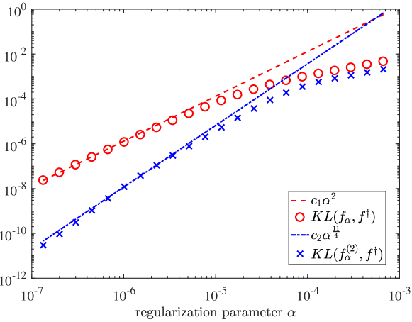
Figure 1: Predicted and computed approximation error for standard and iterated maximum entropy regularization.

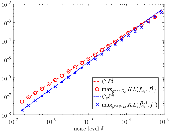
Figure 2: Predicted and computed convergence rates for standard and iterated maximum entropy regularization.

Discussion of the results:    Figure 1 shows the approximation error as a function of $\alpha$, i.e. $\operatorname{KL}(f_{\alpha},f^{\dagger})$ where $f_{\alpha}$ and $f_{\alpha}^{(2)}$, rsp., are the reconstructions for exact data $g^{\mathrm{obs}}=g^{\dagger}$. The two dashed lines indicate the corresponding asymptotic convergence rates predicted by our theory, which are in good agreement with the empirical results. Note that the saturation effect limits the convergence of the standard maximum entropy estimator $f_{\alpha}=f_{\alpha}^{(1)}$ to the maximal rate $\operatorname{KL}(f_{\alpha},f^{\dagger})=\mathcal{O}(\alpha^{2})$. Iterating maximum entropy estimation yields a clear improvement to $\operatorname{KL}(f_{\alpha}^{(2)},f^{\dagger})=\mathcal{O}(\alpha^{s/a})=\mathcal{O}(\alpha^{11/4})$.

Figure 2 displays the convergence rates with respect to the noise level $\delta$ for the a-priori choice rule of $\alpha$ described above. Of course, in practice one would rather use some a-posteriori stopping rule such as the Lepskii balancing principle, but this is not in the scope of this paper. Again, we observe very good agreement of the empirical rate $\operatorname{KL}(\hat{f}_{\alpha},f^{\dagger})=\mathcal{O}(\delta^{4/3})$ with the maximal rate for non-iterated maximum entropy regularization, as well as agreement of the rate $\operatorname{KL}(\hat{f}_{\alpha}^{(2)},f^{\dagger})=\mathcal{O}(\delta^{2s/(s+a)})=\mathcal{O}(\delta^{22/15})$ of the Bregman iterated estimator $\hat{f}_{\alpha}^{(2)}$ with the rate predicted by Theorem 5.7.

7 Discussion and outlook

We have shown that variational source conditions can yield convergence rates of arbitrarily high order in Hilbert spaces. Furthermore we have used this approach to show third order convergence rates in Banach spaces for the first time.

This naturally leads to the question about arbitrarily high order convergence rates in Banach spaces. There are some difficulties that prevented us from going to fourth order convergence rates. The approach in Section 4 relies on comparison with the convergence rates for the dual variables. As the dual problem to generalized Tikhonov regularization is again some form of generalized Tikhonov regularization, it has finite qualification. Therefore, it does not seem straightforward to get to higher orders with this approach. For the approach in Section 3 one needs some relation between $\Delta_{\mathcal{R}}(\hat{f}_{\alpha}^{(2)},f^{\dagger})$ and $\Delta_{\mathcal{R}}(\hat{f}_{\alpha},f^{\dagger}-\alpha^{q^{*}-1}\overline{\omega})$, which is established in (17) and (18) using the polarization identity. However, this identity only has generalizations in the form of inequalities in Banach spaces.

We hope that the tools provided in this paper will initialize a further development of regularization theory in Banach spaces concerning higher order convergence rates. Topics of future research may include other regularization methods (e.g. iterative methods), verifications of higher order variational source conditions for non-smooth penalty terms, stochastic noise models, more general data fidelity terms, or nonlinear forward operators.

Appendix A Duality mappings and an inequality by Xu and Roach

In this appendix we derive a lower bound on Bregman distances in terms of norm powers from more general inequalities by Xu and Roach. First recall the following definitions (see e.g. [32]):

Definition A.1.

The modulus of convexity $\delta_{\mathcal{Y}}\colon(0,2]\to[0,1]$ of the space $\mathcal{Y}$ is defined by

$$\delta_{\mathcal{Y}}(\varepsilon):=\inf\{1-\left\|y+\tilde{y}\right\|/2:y,\tilde{y}\in\mathcal{Y},\left\|y\right\|=\left\|\tilde{y}\right\|=1,\left\|y-\tilde{y}\right\|=\varepsilon\}.$$

The modulus of smoothness $\rho_{\mathcal{Y}}\colon(0,\infty)\to(0,\infty)$ of $\mathcal{Y}$ is defined by

$$\rho_{\mathcal{Y}}(\tau):=\sup\{(\left\|y+\tilde{y}\right\|+\left\|y-\tilde{y}\right\|)/2-1:y,\tilde{y}\in\mathcal{Y},\left\|y\right\|=1,\left\|\tilde{y}\right\|=\tau\}.$$

The space $\mathcal{Y}$ is called uniformly convex if $\delta_{\mathcal{Y}}(\varepsilon)>0$ for every $\varepsilon>0$. It is called uniformly smooth if $\lim_{\tau\to 0}\rho_{\mathcal{Y}}(\tau)/\tau=0.$ The space $\mathcal{Y}$ is called $r$-convex (or convex of power type $r$) if there exists a constant $K>0$ such that $\delta_{\mathcal{Y}}(\varepsilon)\geq K\varepsilon^{r}$ for all $\varepsilon>0$. Similarly, it is called $s$-smooth (or smooth of power type $s$) if $\rho_{\mathcal{Y}}(\tau)\leq K\tau^{s}$ for all $\tau>0$.

As an example we mention that $L_{p}$ spaces with $1<p<\infty$ are $\min(p,2)$-smooth and $\max(p,2)$-convex. It is known (see [19]) that every Banach space, which is either uniformly smooth or uniformly convex, allows an equivalent norm with respect to which it is $r$-convex and $s$-smooth with $1<s\leq 2\leq r<\infty$. By [32, Proposition 1.e.2] we know that $\mathcal{Y}^{*}$ is $s^{*}$-convex and $r^{*}$-smooth.

Recall that $\mathcal{S}=\frac{1}{q}\left\|\cdot\right\|_{\mathcal{Y}}^{q}$ with $q>1$. By [8, Chap.1, Theorem 4.4] we have $\partial\mathcal{S}(y)=J_{q,\mathcal{Y}}(y)$, where $J_{q,\mathcal{Y}}$ is the duality mapping given by

$$J_{q,\mathcal{Y}}(y) :=\left\{\omega\in\mathcal{Y}^{*}:\left\langle\omega,y\right\rangle=\left\|\omega\right\|\left\|y\right\|,\left\|\omega\right\|=\left\|y\right\|^{q-1}\right\}.$$ (57)

$J_{q,\mathcal{Y}}$ is $(q-1)$-homogeneous, i.e. for all $\lambda\in\mathbb{R}$ we have

$$J_{q,\mathcal{Y}}(\lambda y)=\operatorname{sgn}(\lambda)|\lambda|^{q-1}J_{q,\mathcal{Y}}(y).$$ (58)

We assume that $\mathcal{Y}$ is $q$-smooth, $J_{q,\mathcal{Y}}$ is single-valued [8, Chap.1, Corollary 4.5], and we can drop superscripts in Bregman distances.

Lemma A.2 (Xu-Roach).

Let $\mathcal{Y}$ be an $r$-convex Banach space and $\mathcal{S}=\frac{1}{q}\left\|\cdot\right\|_{\mathcal{Y}}^{q}$ for some $q>1$. Then there exist a constant $c_{q,\mathcal{Y}}>0$ depending only on $q$ and the space $\mathcal{Y}$ such that for all $x,y\in\mathcal{Y}$ we have

$$\Delta_{\mathcal{S}}(x,y)\geq\begin{cases}c_{q,\mathcal{Y}}\max\{\|y\|,\|x-y\|\}^{q-r}\|x-y\|^{r}&\text{if }q\leq r,\\ c_{q,\mathcal{Y}}\|y\|^{q-r}\|x-y\|^{r}&\text{if }q\geq r.\end{cases}$$

Proof.

Let $q\leq r$. By [42, Theorem 1] there exists a constant $C$ depending only on $q$ and $\mathcal{Y}$ such that

$$\Delta_{\mathcal{S}}(x,y)\geq C\int_{0}^{1}\frac{t^{r-1}}{2^{r}}\max\{\|y\|,\|y+t(x-y)\|\}^{q-r}\|x-y\|^{r}\mathop{}\!\mathrm{d}t.$$

As $\max\{\|y\|,{\|y+t(x-y)\|}\}\leq 2\max\{\|y\|,\|x-y\|\}$ for all $t\in[0,1]$ and $q-r\leq 0$, we conclude

$$\Delta_{\mathcal{S}}(x,y)\geq 2^{q-r}C\max\{\|y\|,\|x-y\|\}^{q-r}\|x-y\|^{r}\int_{0}^{1}\frac{t^{r-1}}{2^{r}}\mathop{}\!\mathrm{d}t.$$

This shows the lower bound with $c_{q,\mathcal{Y}}:=2^{q-r}C\int_{0}^{1}\frac{t^{r-1}}{2^{r}}\mathop{}\!\mathrm{d}t>0$ in this case. If $r<q$ we have $\max\{\|y\|,\|y+t(x-y)\|\}^{q-r}\geq\|y\|^{q-r}$, so that the claim follows as above.

Acknowledgements.

We would like to thank two anonymous referees for their comments, which helped to improve the paper. Financial support by Deutsche Forschungsgemeinschaft through grant CRC 755, project C09, and RTG 2088 is gratefully acknowledged.

References

- [1] V. Albani, P. Elbau, M. V. de Hoop, and O. Scherzer. Optimal convergence rates results for linear inverse problems in hilbert spaces. Numerical Functional Analysis and Optimization, 37(5):521–540, feb 2016.
- [2] Roman Andreev, Peter Elbau, Maarten V. de Hoop, Lingyun Qiu, and Otmar Scherzer. Generalized convergence rates results for linear inverse problems in hilbert spaces. Numerical Functional Analysis and Optimization, 36(5):549–566, mar 2015.
- [3] J. M. Borwein and A. S. Lewis. Convergence of best entropy estimates. SIAM J. Optim., 1(2):191–205, 1991.
- [4] M. Burger, E. Resmerita, and L. He. Error estimation for Bregman iterations and inverse scale space methods in image restoration. Computing, 81(2-3):109–135, 2007.
- [5] Martin Burger and Stanley Osher. Convergence rates of convex variational regularization. Inverse Problems, 20(5):1411–1421, 2004.
- [6] Y. Censor and S. A. Zenios. Proximal minimization algorithm with -functions. J. Optim. Theory Appl., 73(3):451–464, 1992.
- [7] Gong Chen and Marc Teboulle. Convergence analysis of a proximal-like minimization algorithm using Bregman functions. SIAM J. Optim., 3(3):538–543, 1993.
- [8] I. Cioranescu. Geometry of Banach Spaces, Duality Mappings and Nonlinear Problems, volume 62 of Mathematics and its Applications. Kluwer Academic Publishers, 1990.
- [9] Ronald A. DeVore and Vasil A. Popov. Interpolation of Besov spaces. Trans. Amer. Math. Soc., 305(1):397–414, 1988.
- [10] Jonathan Eckstein. Nonlinear proximal point algorithms using Bregman functions, with applications to convex programming. Math. Oper. Res., 18(1):202–226, 1993.
- [11] P P B Eggermont. Maximum entropy regularization for Fredholm integral equations of the first kind. SIAM J. Math. Anal., 24:1557–1576, 1993.
- [12] Ivar Ekeland and Roger Temam. Convex Analysis and Variational Problems. North-Holland Publishing Company, Amsterdam, Oxford, 1976.
- [13] H W Engl and G Landl. Convergence rates for maximum entropy regularization. SIAM J. Numer. Anal., 30:1509–1536, 1993.
- [14] Heinz W. Engl, Martin Hanke, and Andreas Neubauer. Regularization of inverse problems, volume 375 of Mathematics and its Applications. Kluwer Academic Publishers Group, Dordrecht, 1996.
- [15] Jens Flemming. Generalized Tikhonov regularization and modern convergence rate theory in Banach spaces. Shaker Verlag, Aachen, 2012.
- [16] K. Frick and M. Grasmair. Regularization of linear ill-posed problems by the augmented Lagrangian method and variational inequalities. Inverse Problems, 28(10):104005, 16, 2012.
- [17] Klaus Frick, Dirk A. Lorenz, and Elena Resmerita. Morozov’s principle for the augmented lagrangian method applied to linear inverse problems. Multiscale Modeling & Simulation, 9(4):1528–1548, oct 2011.
- [18] Klaus Frick and Otmar Scherzer. Regularization of ill-posed linear equations by the non-stationary augmented Lagrangian method. J. Integral Equations Appl., 22(2):217–257, 2010.
- [19] G. Godefroy. Renormings in Banach spaces. In J. Lindenstrauss W.B. Jonson, editor, Handbook of the Geometry of Banach Spaces, volume 1, page pp. 781–835. Elsevier Science, Amsterdam, 2001.
- [20] Markus Grasmair. Generalized Bregman distances and convergence rates for non-convex regularization methods. Inverse Problems, 26:115014 (16pp), 2010.
- [21] Markus Grasmair. Variational inequalities and higher order convergence rates for Tikhonov regularisation on Banach spaces. Journal of Inverse and Ill-Posed Problems, 21(3):379–394, Jan 2013.
- [22] C W Groetsch. The Theory of Tikhonov regularization for Fredholm equations of the first kind. Pitman, Boston, 1984.
- [23] B. Hofmann, B. Kaltenbacher, C. Pöschl, and O. Scherzer. A convergence rates result for Tikhonov regularization in Banach spaces with non-smooth operators. Inverse Problems, 23(3):987–1010, 2007.
- [24] B. Hofmann and M. Yamamoto. On the interplay of source conditions and variational inequalities for nonlinear ill-posed problems. Applicable Analysis, 89(11):1705–1727, 2010.
- [25] Thorsten Hohage and Frederic Weidling. Verification of a variational source condition for acoustic inverse medium scattering problems. Inverse Problems, 31(7):075006, 14, 2015.
- [26] Thorsten Hohage and Frederic Weidling. Characterizations of variational source conditions, converse results, and maxisets of spectral regularization methods. SIAM J. Numer. Anal., 55(2):598–620, 2017.
- [27] Thorsten Hohage and Frank Werner. Convergence rates for inverse problems with impulsive noise. SIAM J. Numer. Anal., 52(3):1203–1221, 2014.
- [28] Thorsten Hohage and Frank Werner. Inverse problems with Poisson data: statistical regularization theory, applications and algorithms. Inverse Problems, 32:093001, 56, 2016.
- [29] Jon Johnsen. Pointwise multiplication of Besov and Triebel-Lizorkin spaces. Math. Nach., 175:85–133, 1995.
- [30] Barbara Kaltenbacher and Bernd Hofmann. Convergence rates for the iteratively regularized Gauss-Newton method in Banach spaces. Inverse Problems, 26(3):035007, 21, 2010.
- [31] Djalil Kateb. Fonctions qui opèrent sur les espaces de Besov. Proc. Amer. Math. Soc., 128(3):735–743, 2000.
- [32] J. Lindenstrauss and L. Tzafriri. Classical Banach Spaces II: Function Spaces (Ergebnisse Der Mathematik Und Ihrer Granzgebiete, Vol 97). Springer-Verlag, 1979.
- [33] Andreas Neubauer. On converse and saturation results for Tikhonov regularization of linear ill-posed problems. SIAM Journal on Numerical Analysis, 34(2):517–527, Apr 1997.
- [34] Andreas Neubauer, Torsten Hein, Bernd Hofmann, Stefan Kindermann, and Ulrich Tautenhahn. Improved and extended results for enhanced convergence rates of Tikhonov regularization in Banach spaces. Applicable Analysis, 89(11):1729–1743, Nov 2010.
- [35] Stanley Osher, Martin Burger, Donald Goldfarb, Jinjun Xu, and Wotao Yin. An iterative regularization method for total variation-based image restoration. Multiscale Modeling & Simulation, 4(2):460–489, Jan 2005.
- [36] Elena Resmerita. Regularization of ill-posed problems in Banach spaces: convergence rates. Inverse Problems, 21(4):1303–1314, 2005.
- [37] Elena Resmerita and Otmar Scherzer. Error estimates for non-quadratic regularization and the relation to enhancement. Inverse Problems, 22(3):801–814, 2006.
- [38] Otmar Scherzer, Markus Grasmair, Harald Grossauer, Markus Haltmeier, and Frank Lenzen. Variational Methods in Imaging: 167 (Applied Mathematical Sciences). Springer New York, 2008.
- [39] J Skilling, editor. Maximum entropy and Bayesian methods. Kluwer, Dordrecht, 1989.
- [40] Hans Triebel. Interpolation theory, function spaces, differential operators, volume 18 of North-Holland Mathematical Library. North-Holland Publishing Co., Amsterdam-New York, 1978.
- [41] Hans Triebel. Theory of Function Spaces II. Birkhäuser, Basel, 1992.
- [42] Zong-Ben Xu and G.F Roach. Characteristic inequalities of uniformly convex and uniformly smooth banach spaces. Journal of Mathematical Analysis and Applications, 157(1):189–210, May 1991.