Scalar and Tensor Glueballs as Gravitons

Abstract

The bottom-up approach of the AdS/CFT correspondence leads to the study of field equations in an $AdS_{5}$ background and from their solutions to the determination of the hadronic mass spectrum. We extend the study to the equations of $AdS_{5}$ gravitons and determine from them the glueball spectrum. We propose an original presentation of the results which facilitates the comparison of the various models with the spectrum obtained by lattice QCD. This comparison allows to draw some phenomenological conclusions.

I Introduction

Quantum Chromodynamics (QCD), the theory of the strong interactions, has eluded an analytical solution since its formulation Fritzsch:1973pi . One of the aspects of QCD which has attracted much attention is the glueball spectrum Fritzsch:1975wn ; Mathieu:2008me . In an attempt to understand this theory a procedure to extend the AdS/CFT correspondence breaking conformal invariance and supersymmetry was proposed Maldacena:1997re ; Witten:1998qj ; Witten:1998zw ; Gubser:1998bc . In this so called top-down approach the glueball spectrum has been studied Csaki:1998qr ; Constable:1999gb ; Brower:2000rp ; Vento:2017ice . The AdS geometry of the dual theory is an AdS-black-hole geometry where the horizon plays the role of an infrared (IR) brane.

One relevant feature found in ref.Brower:2000rp is that the graviton of $AdS_{7}$, not the dilaton, corresponds to the lightest scalar glueball. This feature is in good agreement with the lattice QCD spectrum were the lightest scalar glueball has a much lower mass than its immediate excitation which is almost degenerate with the tensor glueball Mathieu:2008me ; Bali:1993fb ; Morningstar:1999rf ; Vaccarino:1999ku ; Lee:1999kv ; Bali:2000vr ; Hart:2001fp ; Lucini:2004my ; Chen:2005mg ; Gregory:2012hu ; Lucini:2001ej . This observation motivates the present investigation.

A different strategy based of the AdS/CFT correspondence, the so-called botton-up approach starts from QCD and attempts to construct a five-dimensional holographic dual. One implements duality in nearly conformal conditions defining QCD on the four dimensional boundary and introducing a bulk space which is a slice of $AdS_{5}$ whose size is related to $\Lambda_{QCD}$ Polchinski:2000uf ; Brodsky:2003px ; Erlich:2005qh ; DaRold:2005mxj . This is the so called hard-wall approximation. Later on, in order to reproduce the Regge trajectories, the so called soft-wall approximation was introduced Karch:2006pv ; reggenew . Within the bottom-up strategy and in both, hard-wall and the soft-wall approaches, glueballs arising from the correspondence of fields in $AdS_{5}$ have been studied BoschiFilho:2002vd ; BoschiFilho:2005yh ; Colangelo:2007pt ; Forkel:2007ru ; Li:2013pta ; Li:2013oda .

In this scenario, the purpose of this investigation is to find the role of the $AdS_{5}$ graviton in the bottom-up approach. We study the spectrum of the scalar and tensor components of the $AdS_{5}$ graviton establishing a correspondence with the glueball spectrum of lattice QCD Morningstar:1999rf ; Lucini:2004my ; Chen:2005mg shown in Table 1.

	$0^{++}$	$2^{++}$	$0^{++}$	$2^{++}$	$0^{++}$	$0^{++}$
MP	$1730\pm 94$	$2400\pm 122$	$2670\pm 222$
YC	$1719\pm 94$	$2390\pm 124$
LTW	$1475\pm 72$	$2150\pm 104$	$2755\pm 124$	$2880\pm 164$	$3370\pm 180$	$3990\pm 277$

Table 1: Glueball masses (MeV) from lattice calculations MP Morningstar:1999rf , YC Chen:2005mg and LTW Lucini:2004my . We have not included the lattice results from the unquenched calculation Gregory:2012hu to be consistent, which are in agreement with the shown results within errors.

We will also show in our figures for completeness the $N\rightarrow\infty$ limit of the lightest scalar glueball. The mass of the other glueballs do not change much in this limit Lucini:2001ej ; Lucini:2004my as shown in table 2.

m(SU(3))/m(SU($\infty$))	$0^{++}$		$0^{++*}$		$2^{++}$
Continuum	$1.07\pm 0.04$		$0.94\pm 0.04$		$1.00\pm 0.03$
Smallest lattice	$1.17\pm 0.05$		$1.00\pm 0.04$		$0.99\pm 0.04$

Table 2: Ratios of glueball masses for N=3 and very large N as shown in ref. Lucini:2004my ; Lucini:2001ej .

In the next sections we proceed to study the graviton in the hard-wall and soft-wall approaches to $AdS_{5}$ and compare the results with previous calculations with scalar and tensor fields. The graviton arises from Einstein’s equations, while the variational approach on the field Lagrangian gives rise to the equations of motion for the fields. Thereafter we match the spectra obtained from these different models with the lattice QCD (LQCD) glueball spectrum Morningstar:1999rf ; Chen:2005mg ; Lucini:2004my and extract conclusions.

II Glueballs as hard-wall gravitons

According to AdS/CFT correspondence massless scalar string states are dual to boundary scalar glueball operators Witten:1998zw ; Gubser:1998bc ; Polchinski:2000uf . On the other hand scalar string excitations with mass $\mu$ couple to boundary operators of dimension $\Delta=2+\sqrt{4+(\mu R)^{2}}$. Glueball operators with spin $J$ have dimension $\Delta=4+J$, thus a consistent coupling between string states with mass $\mu$ and glueball operators with spin $J$ requires $(\mu R)^{2}=J(J+4)$. The glueball operators are massless and respecting conformal invariance. Once we introduce a size in the AdS space there is an infrared cut off in the boundary which is proportional to $1/\Lambda_{QCD}$, explicitly breaking conformal invariance. The presence of the slice implies an infinite tower of discrete modes for the bulk states. These bulk discrete modes are related to the masses of the non-conformal glueball operators.

In the bottom-up approach, supergravity fields in the $AdS_{5}$ slice times a compact $S_{5}$ space are considered an approximation for a string dual to QCD. The metric of this space can be written as

$$ds^{2}=\frac{R^{2}}{z^{2}}(dz^{2}+\eta_{\mu\nu}dx^{\mu}dx^{\nu})+R^{2}d\Omega_{5},$$ (1)

where $\eta_{\mu\nu}$ is the Minkowski metric and the size of the slice in the holographic coordinate $0<z<z_{max}$ is related to the scale of QCD, $z_{max}=\frac{1}{\Lambda_{QCD}}$. The equation of motion for the scalar field with mass $\mu$ in $AdS_{5}$ is obtained from the Lagrangian of a free scalar in the curved background and leads to Witten:1998zw ; Gubser:1998bc

$$\partial_{z}^{2}\Phi-\frac{3}{z}\partial_{z}\Phi+\eta_{\mu\nu}\partial^{\mu}\partial^{\nu}\Phi-\frac{(\mu R)^{2}}{z^{2}}\Phi=0.$$ (2)

Motivated by the work of ref.Brower:2000rp in the top-down approach, we study the contribution of the scalar component of the massless graviton in the sliced $AdS_{5}$ geometry. Writing the metric as $g_{ab}=\bar{g}_{ab}+h_{ab}$ where $\bar{g}_{ab}$ is the background metric Eq.(1), which is a solution of Einstein’s equations, we obtain for the perturbation $h$ linearizing Einstein’s equations

$$-{1\over 2}h_{ab;c}^{;c}-{1\over 2}h^{c}_{c;ab}+{1\over 2}h_{ac;b}^{;c}+{1\over 2}h_{bc;a}^{;c}+4h_{ab}=0,$$ (3)

which are the field equations for the graviton. Choosing the gauge where the only non vanishing component is

$$h_{tt}=(z^{-2}-z^{2})\phi(z)e^{-mx_{3}}~{},$$ (4)

where $m$ is the mass parameter. Substituting this ansatz into Eq.(3) we obtain Eq.(2) for a plane wave solution $\Phi(x,z)\sim e^{-iP\cdot x}\phi(z)$ with $P^{2}=-M^{2}$ and $\mu R=0$,

$$\frac{d^{2}\phi}{dz^{2}}-3\frac{d\phi}{dz}+M^{2}\phi=0$$ (5)

Thus the scalar graviton equation is exactly the same equation as that for the massless scalar fields dual to the scalar glueballs BoschiFilho:2002vd ; BoschiFilho:2005yh ; Colangelo:2007pt .

Let us now find the perturbation to Einstein’s equations for the tensor component of the graviton. In this case we choose the gauge

$$h_{ij}=q_{ij}T(z)e^{-mx_{3}},$$ (6)

being $i,j=1,2$ and $q_{ij}$ a generic constant traceless-symmetric matrix. The result of this calculation for $T(z)$ is also Eq.(5). Thus the scalar graviton and tensor graviton components lead to the same equation. The two components are degenerate.

The spectrum of the graviton coincides with that of the scalar fields and the tensor graviton with the tensor fields if we add a mass term $(\mu R)^{2}=12$ if we use the same boundary conditions. Let us recall these solutions.

The plane wave solutions

$$\Phi(x_{\mu},z)=C_{k}e^{-iPx}z^{2}J_{2}(u_{k}z),$$ (7)

with the following boundary conditions,

Dirichlet $$J_{2}(\chi_{k}) =0,$$

Neumann $$J_{1}(\xi_{k}) =0,$$ (8)

determine the scalar spectrum. Here $J_{2}$ and $J_{1}$ are Bessel functions, for the Dirichlet modes $u_{k}=\chi_{k}\Lambda_{QCD}$, while for the Neumann modes $u_{k}=\xi_{k}\Lambda_{QCD}$ and $k$ labels the energy modes. The corresponding solutions for the mass of the glueballs in dimensionless units of $\Lambda_{QCD}$ are given by the zeros of the corresponding Bessel functions. The energy modes of the scalar glueball are shown in Table 3.

k	1	2	3	4	5	…
D scalar	5.136	8.417	11.620	14.796	17.960	…
N scalar	3.832	7.016	10.173	13.324	16.471	…

Table 3: Energy modes for the scalar glueball in the hard-wall model with Dirichlet (D) and Neumann (N) boundary conditions.

For the tensor modes according to duality we simply have to add the mass term $(\mu R)^{2}=J(J+4)$. Considering again plane wave solutions the spectrum is given by ,

Dirichlet	$J_{n}(\chi_{n,k})=0$ ,
Neumann	$(2-n)J_{n}(\xi_{n,k})+\xi_{n,k}J_{n-1}(\xi_{n,k})=0$ ,

(9)

where $J_{n}$ are Bessel functions, $n=2+J$ and $k$ labels the modes.

We show the tensor modes in Table 4 reggenew ; BoschiFilho:2005yh .

k	1	2	3	4	5	…
D tensor	7.588	11.065	14.373	17.616	20.827	…
N tensor	5.981	9.537	12.854	16.096	19.304	…

Table 4: Energy modes for the tensor field in the hard-wall model with Dirichlet (D) and Neumann (N) boundary conditions.

We proceed to compare this $AdS_{5}$ spectrum to the quenched LQCD glueball spectrum Morningstar:1999rf ; Lucini:2004my ; Chen:2005mg in Fig.1. To this aim, we fix the scale of the $AdS_{5}$ calculation by performing a best fit to the lowest glueball state. Once the $AdS_{5}$ spectrum is plotted with this initial scale we seed the data into the plot attributing the mode numbers to the different glueball states. Finally we modify slightly the scale of our original fit to get a best fit to the data. Note that we plot two masses for the lightest glueballs, which correspond to the ones obtained by LQCD and its large $N$ limit as shown in Table 2 Lucini:2001ej ; Lucini:2004my .

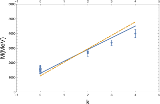
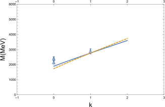
Figure 1: Gluebal spectrum obtained in the hard-wall model. The figure on the left shows the fit to the scalar (J=0) glueball spectrum. The figure on the right shows fit to the tensor ($J=2$) glueball spectrum. The solid lines correspond to Dirichlet boundary conditions and the dashed lines to Neumann boundary conditions. The full circles represent the scalar LQCD masses, the squares the large N limit scalar LQCD masses and the triangles the tensor LQCD masses.

The figure to the left shows the Dirichlet and Neumann fit to the scalar spectrum. We have skipped the $k=1$ mode because its value is $2713$ MeV is too high for a reasonable fit. The figure on the right shows the fit to the tensor glueballs which has been obtained incorporating the mass term. Note that since the scale is the same for scalar and tensor we have to get a best fit to both data sets.

While the relation between the scalar graviton component and the scalar glueball is analogous to that of the scalar field: same equations and no $AdS_{5}$ mass, the tensor graviton is not unless we introduce artificially a mass term. However the LQCD spectrum is telling us that the second tensor glueball and the second scalar are almost degenerate. Moreover by looking at the modes in Tables 3 and 4 one realizes that the second scalar mode and the first tensor modes are almost degenerate, very much so in the Dirichlet case. Guided by this almost degeneracy of the scalar and tensor LQCD masses and of the degenerate scalar and tensor modes we plot both scalar and tensor modes following the massless equation, since the graviton equations for scalar and tensor are degenerate. To get a reasonable fit to the data, we skip for the tensor the $k=0$ mode, i.e., the lowest tensor glueball at $2313$ MeV is ascribed to $k=1$ and since the next scalar glueball, the $2713$ MeV, is almost degenerate with the $2880$ MeV tensor glueball we assign to it the $k=2$ mode number. The result is shown in Fig. 2. The fit is quite good with only one curve for scalar and tensor glueballs. The mode skipping in the case of the tensor is like a mass gap as we shall see in the soft-wall models.

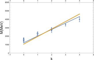
Figure 2: Gluebal spectrum obtained in the hard-wall model. We plot the modes of the massless equation which represents the degeneracy of the scalar and tensor gravitons skipping the $k=0$ mode for the tensor and the $k=1$ mode for the scalar. The solid lines correspond to Dirichlet boundary conditions and the dashed lines to Neumann boundary conditions. The full circles represent the scalar LQCD masses, the squares the large N limit scalar LQCD masses and the triangles the tensor LQCD masses.

III Glueballs as soft-wall gravitons

Another scheme to determine the spectrum of QCD from $AdS_{5}$ has been a mechanism for a gravitational background which cuts-off smoothly in the holographic coordinate. The mechanism introduced some time ago for that purpose, capable of reproducing the Regge behavior of mesons, consists in incorporating a dilaton field $\delta$ and a metric $g_{MN}$ with characteristic properties Karch:2006pv . In this formalism the glueballs are described by 5d fields propagating in this background with the action given by

$$\mathcal{I}=\int{d^{5}x\sqrt{-g}e^{-\delta}\mathcal{L}},$$ (10)

where $\mathcal{L}$ is the lagrangian density describing the dynamics of the scalar fields, $\delta$ the dilaton whose mission is to soften the $z$ cut-off,

$$\delta(z)=\beta^{2}z^{2}.$$ (11)

and $g=\det{g_{ab}}$, where $g_{ab}$ is the $AdS_{5}$ metric defined in Eq. (1) Colangelo:2007pt . Since our aim is to find the glueballs associated with the $AdS$ graviton without changing the results for conventional hadrons, we generalize the metric to

$$g_{ab}(z)=e^{-\alpha^{2}(z^{2}/R^{2})}\frac{R^{2}}{z^{2}}(-1,1,1,1,1).$$ (12)

Eq. (12) is a modification of the metric suitable for enriching the dynamics of the $AdS$ graviton. These type of metrics have been used to explore heavy quark physics Andreev:2006ct ; White:2007tu ; Bruni:2018dqm . In order to implement the condition of Regge trajectories used in previous calculation Karch:2006pv ; Colangelo:2007pt we must impose

$$\frac{3\alpha^{2}}{2}+\beta^{2}=1.$$ (13)

Note that the change of metric affects the lagrangian term in the action leading to an additional multiplicative factor $e^{\alpha^{2}z^{2}}$ in the integral which is the reason for the factor $3/2$ in Eq. (13). Such a choice for the metric produces a Lagrangian for a scalar field that is identical to that of Eq. (10) and will lead to the same equations of motion for the fields. We add no new degrees of freedom. However, the graviton equations of motion change.

Given these restrictions, the spectra for the glueballs, arising from the scalar and tensor fields, using $R=1$ in Eq. (12), are those of ref. Colangelo:2007pt , i.e., $M^{2}_{J}=4k+4+2\sqrt{4+J(J+4)},\;k=0,1,\ldots$, for even $J$. We rewrite these equations for scalar and tensor in a single expression,

$$M^{2}=4k+8,$$ (14)

where $k=0,1,...$ for the scalar modes and $k=1,2,..$ for the tensor modes. One should notice that the addition of the mass term to the tensor is equivalent to skipping the $k=0$ mode. In this model the phenomenological procedure for the spectra discussed for the hard-wall model is perfectly realized. These solutions correspond also to the graviton with the old metric Eq. (1), i.e. $\alpha=0$

Let us find the spectrum for the scalar component of the graviton by solving the Einstein’s equations corresponding to the new metric Eq. (12). Using $R=1$ and the same gauge Eq.(4) the mode equation becomes

$$\frac{d^{2}\phi}{dz^{2}}+\left(\alpha^{2}z-\frac{3}{z}\right)\frac{d\phi}{dz}+\left(\frac{8}{z^{2}}+6\alpha^{2}+M^{2}+4\alpha^{2}z^{2}\right)\phi-\frac{8}{z^{2}}e^{-\alpha^{2}z^{2}}\phi=0.$$ (15)

Note that for $\alpha^{2}=0$ this equation reduces to Eq.(5). From this one can obtain a Schrödinger type equation,

$$-\Psi^{\prime\prime}(z)+V_{GS}(z)\Psi(z)=M^{2}\Psi(z),$$ (16)

where

$$V_{GS}(z)=\frac{8e^{\alpha^{2}z^{2}}}{z^{2}}-\frac{17}{4z^{2}}-7\alpha^{2}-\frac{15\alpha^{4}z^{2}}{4}.$$ (17)

In terms of the new variable $\tau=\alpha z/\sqrt{2}$, Eq.(16) becomes

$$-\frac{d^{2}\Psi}{d\tau^{2}}(\tau)+V_{GSS}(\tau)\Psi(\tau)=\Lambda^{2}\Psi(\tau),$$ (18)

where

$$\Lambda^{2}=\frac{2M^{2}}{\alpha^{2}}$$ (19)

and the potential is given by

$$V_{GSS}(\tau)=\frac{8e^{2\tau^{2}}}{\tau^{2}}-\frac{17}{4\tau^{2}}-14-15\tau^{2}.$$ (20)

In order to study the boundary conditions at the origin we Taylor expand the exponential to second order, obtaining a potential whose behavior at small $\tau$ is

$$V_{low}(\tau)\sim\frac{15}{4\tau^{2}}~{},$$ (21)

which leads to a low $\tau$ behavior for the field function

$$\Psi(\tau)\sim\tau^{5/2}.$$ (22)

Note that $\alpha$ is just a scale in the mass equation and that the mode solutions, $\Lambda_{k}$, are independent of its value. For small values of $\tau$ this equation leads to that of ref.Colangelo:2007pt for the scalar field up to an irrelevant constant $\Lambda_{0}^{2}$.

For $\alpha^{2}>0$, the potential is not binding and the corresponding solutions for the eigenfunctions are damped oscillations. The well behaved modes appear for $\alpha^{2}<0$. In this case we use the variable $t=i\tau,t>0$ and $a=i\alpha,a^{2}>0$. Eqs.(18), (19) and (20) now become

$$-\frac{d^{2}\Psi}{dt^{2}}(t)+V_{GSS}(t)\Psi(t)=\Lambda^{2}\Psi(t),$$ (23)

where,

$$\Lambda^{2}=\frac{2M^{2}}{a^{2}}$$ (24)

and

$$V_{GSS}(t)=\frac{8e^{2t^{2}}}{t^{2}}-\frac{17}{4t^{2}}+14-15t^{2}.$$ (25)

It is important to note the change of sign in the exponential but also in the constant term which lead to quantized modes solutions. We show in Fig. 3 the eigenfunctions for the first three modes. The corresponding eigenvalues, $\Lambda_{k}$, are given in Table 5. The change of $\tau$ by $t$ corresponds to the change in the asymptotic behaviour to go from a non bound to a bound solution.

For tensor component of the graviton choosing the same gauge Eq.(6) one obtains the same equation as for the scalar component Eqs. (16) and (17).

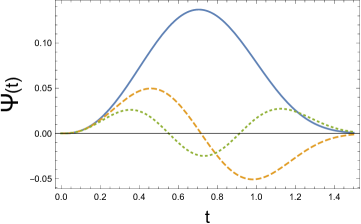
Figure 3: Typical eigenfunctions of the graviton equation for $\alpha^{2}<0$. The solid curve shows the lowest (k=0) mode, the dashed curve that of the first mode (k=1) and the dotted curve that of the the second mode (k=2).

k	0	1	2	4	$\ldots$
scalar graviton	7.341	9.065	10.818	12.568	$\ldots$

Table 5: The scalar modes $\Lambda_{k}$ of the graviton equation in the soft-wall model.

In Table 6 we show the corresponding mass modes $M_{k}$ for scalar and tensor fields Colangelo:2007pt and scalar and tensor graviton components calculated above.

k	0	1	2	4	$\ldots$
scalar field	2.82	3.46	4.00	4.47	$\ldots$
tensor field	3.46	4.00	4.47	4.89	$\ldots$
scalar & tensor graviton	5.19	6.41	7.65	8.89	$\ldots$

Table 6: The mass modes $M_{k}$ for the scalar, tensor and the scalar and tensor graviton components in the soft-wall model.

Let us compare the results of the two soft-wall models studied with the LQCD results. In order to perform such comparison, we fix the scale of the $AdS_{5}$ calculation by performing a best fit to the lattice data of the scalar glueball. Our fit requires a value of $|\alpha|\sim 0.32$ which is close to $0.375$ obtained in ref. Brodsky:2007hb by studying the pion form factor in a soft-wall model, and somewhat smaller that that of ref. Andreev:2006ct , $0.47$, obtained by analyzing heavy quark dynamics also in a soft-wall model.

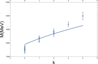
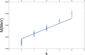
Figure 4: Glueball spectrum obtained by the soft-wall approach. The figure on the left shows the scalar and tensor field results. The figure on the right shows the graviton fit to the glueballs. The symbols as in previous figures

In Fig.4 we plot the graviton and field results for the glueball spectrum, by fitting the scale to the scalar spectrum, and compare them to the LQCD spectrum. We plot again two masses for the lightest glueballs, the one obtained by LQCD and its large $N$ limit. For the fields (left) we see by looking at Eq. (14) that the scalar equation gives the tensor spectrum simply by shifting $k$ in one unit as result of adding a mass to the tensor. From $k=1$ on, the $AdS_{5}$ spectrum of scalar and tensor are degenerate. However, by looking at the lattice spectrum we notice that the degeneracy appears for the $k=2$ tensor, thus we ascribe $k=2$ to the second scalar. An important result of the analysis is as before the missing of a $k=1$ scalar. The overall fit is reasonable but of lower quality than the hard-wall fit with Dirichlet boundary conditions. For the gravitons (right) we proceed as before, a strategy that is now justified by the field equations. We skip the $k=0$ tensor mode and ascribe the first tensor mode to $k=1$. This could be understood as a way of implementing the tensor mass in the graviton approach. Since the scalar and the tensor components of the graviton are also degenerate we ascribe $k=2$ to the second scalar. The fit is of better quality than the conventional soft model approach and the almost linear behavior describes better the data. It is clear that a further modification of the metric in line with refs. White:2007tu ; Bruni:2018dqm is needed to get the adequate slope.

Finally we compare following the same scheme described above the soft graviton with the hard Dirichlet graviton in Fig 5. Both give reasonable fits to the data although their slopes are quite different. The slope in the hard-wall model is too large, while that of the soft-wall model is too small. Thus both require more sophisticated metrics to describe better the data.

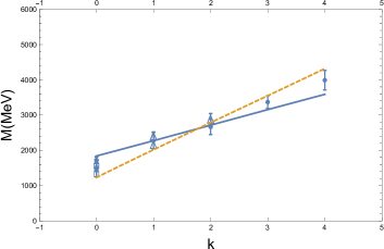
Figure 5: Gluebal spectrum obtained by the soft-wall (solid) and hard-wall (dashed) approaches. The symbols as in previous figures

IV Conclusions

We have discussed the spectrum of the scalar and tensor glueballs under the assumption that in an $AdS_{5}$ approach scalar and tensor components of the graviton might play a significant role corresponding to the lowest lying glueballs. We have studied the problem in hard and soft-wall models.

In the hard-wall model BoschiFilho:2002vd ; BoschiFilho:2005yh the scalar component of the graviton reproduces exactly the same equations as the field approach but the tensor component is degenerate. By fitting an energy scale the results of the model reproduce reasonably well the lattice results, specially so with Dirichlet boundary conditions. The almost linear behavior of the fit is in good agreement with the data.

In the soft-wall approach we study a modification of the dilaton model Colangelo:2007pt with a different metric leading to equations for the graviton which are not the same as those for the field equations. We find new solutions which depend on a metric parameter $\alpha^{2}<0$. The metric grows as $e^{-\alpha^{2}z^{2}}$ which implies that it grows at short distances becoming pure $AdS_{5}$ at infinity leading to a potential which is able to bind. We have solved numerically the equations for the scalar component. The tensor component turns out to be degenerate unless a mass term is added. Both the field and graviton fits to the QCD lattice spectrum reasonable if the first tensor mode is ascribed to $k=1$ and the scalar mode at $k=1$ is skipped. The exact solutions of the field equations give an explanation for the missing $k=0$ tensor mode if we interpret the effect as a tensor mass. In the case of the graviton this missing mode can be interpreted as faking a tensor mass. In both cases we see that the doubling required by $AdS_{5}$ of the $k=1$ glueball is missing. We consider this a prediction of both soft-wall models. If this state does not appear the equivalent $AdS_{5}$ dynamics at low mass has to be more complicated. The graviton solution seems to better reproduce the shape and rise of the lattice glueball spectrum.

The main conclusion of this paper is that we do not need to introduce additional fields into any $AdS_{5}$ model, the gravitons, with the addition of mass terms to satisfy the duality boundary conditions, are able to describe the elementary scalar and tensor glueballs. Fields might be useful to describe more complicated glueball structures.

References

- (1) H. Fritzsch, M. Gell-Mann and H. Leutwyler, Phys. Lett. 47B (1973) 365.
- (2) H. Fritzsch and P. Minkowski, Phys. Lett. 56B (1975) 69.
- (3) V. Mathieu, N. Kochelev and V. Vento, Int. J. Mod. Phys. E 18 (2009) 1 [arXiv:0810.4453 [hep-ph]].
- (4) J. M. Maldacena, Int. J. Theor. Phys. 38 (1999) 1113 [Adv. Theor. Math. Phys. 2 (1998) 231] [hep-th/9711200].
- (5) E. Witten, Adv. Theor. Math. Phys. 2 (1998) 253 [hep-th/9802150].
- (6) E. Witten, Adv. Theor. Math. Phys. 2 (1998) 505 [hep-th/9803131].
- (7) S. S. Gubser, I. R. Klebanov and A. M. Polyakov, Phys. Lett. B 428 (1998) 105 doi:10.1016/S0370-2693(98)00377-3 [hep-th/9802109].
- (8) C. Csaki, H. Ooguri, Y. Oz and J. Terning, JHEP 9901 (1999) 017 [hep-th/9806021].
- (9) N. R. Constable and R. C. Myers, JHEP 9910 (1999) 037 [hep-th/9908175].
- (10) R. C. Brower, S. D. Mathur and C. I. Tan, Nucl. Phys. B 587 (2000) 249 [hep-th/0003115].
- (11) V. Vento, Eur. Phys. J. A 53 (2017) no.9, 185 doi:10.1140/epja/i2017-12378-2 [arXiv:1706.06811 [hep-ph]].
- (12) G. S. Bali et al. [UKQCD Collaboration], Phys. Lett. B 309 (1993) 378 [hep-lat/9304012].
- (13) C. J. Morningstar and M. J. Peardon, Phys. Rev. D 60 (1999) 034509 [hep-lat/9901004].
- (14) A. Vaccarino and D. Weingarten, Phys. Rev. D 60 (1999) 114501 [hep-lat/9910007].
- (15) W. J. Lee and D. Weingarten, Phys. Rev. D 61 (2000) 014015 doi:10.1103/PhysRevD.61.014015 [hep-lat/9910008].
- (16) G. S. Bali et al. [TXL and T(X)L Collaborations], Phys. Rev. D 62 (2000) 054503 doi:10.1103/PhysRevD.62.054503 [hep-lat/0003012].
- (17) A. Hart et al. [UKQCD Collaboration], Phys. Rev. D 65 (2002) 034502 doi:10.1103/PhysRevD.65.034502 [hep-lat/0108022].
- (18) B. Lucini, M. Teper and U. Wenger, JHEP 0406 (2004) 012 doi:10.1088/1126-6708/2004/06/012 [hep-lat/0404008].
- (19) Y. Chen et al., Phys. Rev. D 73 (2006) 014516 [hep-lat/0510074].
- (20) E. Gregory, A. Irving, B. Lucini, C. McNeile, A. Rago, C. Richards and E. Rinaldi, JHEP 1210 (2012) 170 [arXiv:1208.1858 [hep-lat]].
- (21) B. Lucini and M. Teper, JHEP 0106 (2001) 050 doi:10.1088/1126-6708/2001/06/050 [hep-lat/0103027].
- (22) J. Polchinski and M. J. Strassler, hep-th/0003136.
- (23) S. J. Brodsky and G. F. de Teramond, Phys. Lett. B 582 (2004) 211 [hep-th/0310227].
- (24) J. Erlich, E. Katz, D. T. Son and M. A. Stephanov, Phys. Rev. Lett. 95 (2005) 261602 [hep-ph/0501128].
- (25) L. Da Rold and A. Pomarol, Nucl. Phys. B 721 (2005) 79 [hep-ph/0501218].
- (26) A. Karch, E. Katz, D. T. Son and M. A. Stephanov, Phys. Rev. D 74 (2006) 015005 [hep-ph/0602229].
- (27) E. Folco Capossoli and H. Boschi-Filho, Phys. Lett. B 753, 419 (2016)
- (28) H. Boschi-Filho and N. R. F. Braga, JHEP 0305 (2003) 009 doi:10.1088/1126-6708/2003/05/009 [hep-th/0212207].
- (29) H. Boschi-Filho, N. R. F. Braga and H. L. Carrion, Phys. Rev. D 73 (2006) 047901 [hep-th/0507063].
- (30) P. Colangelo, F. De Fazio, F. Jugeau and S. Nicotri, Phys. Lett. B 652 (2007) 73 [hep-ph/0703316].
- (31) H. Forkel, Phys. Rev. D 78 (2008) 025001 [arXiv:0711.1179 [hep-ph]].
- (32) X. F. Li and A. Zhang, Chin. Phys. C 38 (2014) no.1, 013102 [arXiv:1309.7154 [hep-ph]].
- (33) D. Li and M. Huang, JHEP 1311 (2013) 088 [arXiv:1303.6929 [hep-ph]].
- (34) O. Andreev and V. I. Zakharov, Phys. Rev. D 74 (2006) 025023 doi:10.1103/PhysRevD.74.025023 [hep-ph/0604204].
- (35) C. D. White, Phys. Lett. B 652 (2007) 79 doi:10.1016/j.physletb.2007.07.006 [hep-ph/0701157].
- (36) R. C. L. Bruni, E. Folco Capossoli and H. Boschi-Filho, arXiv:1806.05720 [hep-th].
- (37) S. J. Brodsky and G. F. de Teramond, Phys. Rev. D 77 (2008) 056007 doi:10.1103/PhysRevD.77.056007 [arXiv:0707.3859 [hep-ph]].
- (38) V. Vento, Phys. Rev. D 73 (2006) 054006 doi:10.1103/PhysRevD.73.054006 [hep-ph/0401218].