Abstract

We consider an open universe created by bubble nucleation, and study possible effects of our “ancestor vacuum,” a de Sitter space in which bubble nucleation occurred, on the present universe. We compute vacuum expectation values of the energy-momentum tensor for a minimally coupled scalar field, carefully taking into account the effect of the ancestor vacuum by the Euclidean prescription. We pay particular attention to the so-called supercurvature mode, a non-normalizable mode on a spatial slice of the open universe, which has been known to exist for sufficiently light fields. This mode decays in time most slowly, and may leave residual effects of the ancestor vacuum, potentially observable in the present universe. We point out that the vacuum energy of the quantum field can be regarded as dark energy if mass of the field is of order the present Hubble parameter or smaller. We obtain preliminary results for the dark energy equation of state $w(z)$ as a function of the redshift.

1 Introduction

In a theory with multiple vacua, nucleation of bubbles of a true vacuum can occur due to quantum tunneling. If such a theory is coupled to gravity, bubble nucleation provides a mechanism for the creation of an FLRW(Fiedmann-Lemaître-Robertson-Walker) universe. Superstring theory is expected to have a large number of metastable vacua [1, 2, 3] including positive energy de Sitter vacua [4, 5], according to the proposal of the “string landscape” (see e.g., [6] for a review). Although the existence of such vacua has not been proven yet, we consider bubble nucleation to be a viable mechanism to determine initial conditions for our universe.

Understanding of the characteristic features of the universe created by bubble nucleation is of great importance. One of such features is negative spatial curvature [7]. The Coleman-De Luccia instanton [8], which is a semi-classical description of the creation and evolution of a bubble, shows that the universe inside the bubble should have negative curvature. Even though our universe is known to be flat within the margin of error, it is logically possible that there is a finite radius $R_{c}$ of negative curvature. The bound is roughly $R_{c}\gtrsim 10H_{0}^{-1}$ where $H_{0}$ is the current Hubble parameter [9].

Another feature would be the possible signatures in the cosmic microwave background radiation (CMB). The spectrum of the CMB temperature fluctuations is consistent with the nearly scale-invariant spectrum of primordial fluctuations predicted by inflation [10]. However, if the number of e-folds of inflation is finite, we might be able to see deviations from scale invariance due to the evolution of the universe before inflation. Such effects are expected to affect the low-$\ell$ (angular momentum) modes of the power spectrum. The CMB spectrum in the universe created by bubble nucleation has been understood in the 1990’s [11, 12, 13, 15, 16, 17, 18]. The studies on the CMB spectrum after the advent of string landscape include [19, 20, 21, 22, 23]. Although no signature of bubble nucleation has been found in the CMB yet, theoretical study for seeking such a signature is undoubtedly important.

In this paper, we will focus on a third possible feature, related but different from the above two. We will consider how the quantum fluctuations generated before bubble nucleation affect the vacuum energy in the present universe. The universe created by bubble nucleation is surrounded by a parent de Sitter space, which we call the ancestor vacuum (See Fig. 1). The Hubble parameter $H_{A}$ for the ancestor vacuum is typically larger than the value $H_{I}$ for inflation after tunneling. On dimensional grounds, large fluctuations will be generated in the ancestor vacuum. In this paper, we will compute the vacuum expectation value of the energy-momentum tensor of a free scalar field, carefully taking into account the effect of the ancestor vacuum.

To find the vacuum expectation value of the energy-momentum tensor, which is quadratic in the quantum field, we compute the two-point functions of the field and take the coincident-point limit. The two-point functions at early time (in our universe) are obtained by the Euclidean prescription, and their subsequent time-evolution can be studied using the equation of motion for the scalar field.

We will be particularly interested in the contribution from a special mode of fluctuations, the so-called “supercurvature mode,” originally found by M. Sasaki, T. Tanaka and K. Yamamoto [11, 12, 13] . This mode decays more slowly than $e^{-R}$ at large $R$ where $R$ is the geodesic distance, and is not normalizable on the spatial slice $H^{3}$ in the open universe. The supercurvature mode appears if the mass of the scalar field in the ancestor vacuum is small enough. For example, for exactly massless fields, two-point functions remain finite even when two points are infinitely separated on $H^{3}$. Heuristically, such fluctuations can be considered as the super-horizon fluctuations in the ancestor (de Sitter) vacuum, seen from the inside of the bubble [27]. Mathematical reason that a non-normalizable mode can exist in the open universe is that the spatial slice $H^{3}$ is not a global Cauchy surface (see Fig. 1). To quantize the fluctuations, one needs to take a complete set of normalizable modes on a Cauchy surface, such as the surface on the horizonal brown line in Fig. 1. The supercurvature mode appears as a result of analytic continuation of the correlator to the open universe, as we will review in Section 3.

Supercurvature modes decay more slowly than normalizable modes, not only in space but also in time. Thus, it may have a chance to affect our current universe. In previous papers by some of the present authors [28, 29], the evolution of vacuum fluctuations generated during and before inflation has been studied, without taking bubble nucleation into account. The emergence of the supercurvature mode is an interesting phenomenon, special to the universe created by bubble nucleation.

As long as the mass of the scalar field is smaller than the Hubble parameter in our universe, the field value for the supercurvature mode remains nearly constant. This is the well-known freezing of the super-horizon fluctuations; supercurvature modes can always be considered to be outside the horizon. The energy-momentum tensor for this mode behaves similarly to that for cosmological constant. After the Hubble parameter decreases below the mass, the field begins to oscillate, and its energy decays. If there is a field with mass of order the present Hubble parameter $H_{0}$ or smaller, the supercurvature mode of this field will be essentially frozen until today. This gives us an interesting possibility for the realization of dark energy.

The primary purpose of this paper is to explain how to calculate the vacuum expectation value of the energy-momentum tensor in the background with bubble nucleation. To the best of our knowledge, this calculation has not been done before. Another purpose is to show that dark energy can be obtained as a contribution from the supercurvature mode to the vacuum energy.

We consider the fluctuations of a minimally coupled scalar field $\phi$, which is different from the tunneling field $\Phi$. The field $\phi$ does not have the vacuum expectation value, and is treated as a free field in the curved spacetime. We assume the mass $m_{A}$ of $\phi$ in the ancestor vacuum to be sufficiently small relative to the Hubble parameter, $m_{A}\ll H_{A}$, so that a supercurvature mode exists. We allow a possibility that mass $m_{0}$ of $\phi$ in the true vacuum is different from $m_{A}$. (This can be realized e.g., if there is a coupling of the form $\Phi^{2}\phi^{2}$, and the expectation value of $\Phi$ is large in the false vacuum and small in the true vacuum.) It would be natural to assume $m_{0}\ll m_{A}$, since the energy scale in the true vacuum will be typically lower than in the false vacuum.

The order of magnitude of the vacuum energy (derived rigorously below) can be estimated as follows. The expectation value of the field squared $\langle\phi^{2}\rangle$ in the ancestor vacuum goes as $\langle\phi^{2}\rangle\sim H_{A}^{4}/m_{A}^{2}$. This is essentially the same as the well-known expression in pure de Sitter space, which becomes infinitely large in the massless and infinite e-folds limit (see e.g., [35, 36]). If we assume $m_{0}\lesssim H_{0}$, the field value $\langle\phi^{2}\rangle$ is nearly frozen until now, apart from its weak time dependence due to the non-zero $m_{A}$ that may play an important role in observationally distinguishing our mechanism from others. The dominant part of the energy-momentum tensor for the field $\phi$ is the mass term, $\rho\sim m_{0}^{2}\langle\phi^{2}\rangle\sim(m_{0}/m_{A})^{2}H_{A}^{4}$. Then, it is possible to make this of the same order as dark energy, $\rho\sim H_{0}^{2}M_{P}^{2}$ where $M_{P}$ is the (reduced) Planck mass. For instance, if there is a field with $m_{0}\sim H_{0}$, we need $M_{P}/H_{A}\sim H_{A}/m_{A}$ (i.e., $H_{A}$ being the geometric mean of $M_{P}$ and $m_{A}$), which does not seem particularly difficult to satisfy.

In this scenario we need an ultra-light field with mass $m_{0}\sim H_{0}\sim 10^{-33}{\rm eV}$. Thus, this may not be regarded as a “natural” solution to the cosmological constant problem [37]. Nevertheless, we believe the detailed study is worthwhile, especially in view of the proposal of the “string axiverse,” which states that there is a large number of axion-like particles with mass ranging down to $m_{0}\sim H_{0}$ [38].

The idea of realizing dark energy as the vacuum energy of an ultra-light field is not essentially new. See e.g., [38, 39, 40, 30, 29, 33, 41] for previous works. Summaries of this topic can be found in review articles [42, 43]. The effect of bubble nucleation has not been considered previously. At the end of this paper, we will comment on the possible observable effects, which could be regarded as a signature of our mechanism.

This paper is organized as follows. In Section 2, we review the Coleman-De Luccia instanton, which describes the nucleation and the evolution of a bubble in de Sitter space (the ancestor vacuum). In Section 3, we review the calculation of correlation functions of a scalar field based on analytic continuation from the Euclidean space. Using this prescription, we obtain the correlators in the early-time limit in the open universe. In Section 4, we compute the expectation value of the energy-momentum tensor by taking the coincident-point limit of the two-point function obtained in the previous section. In particular, we study the mass term in the energy-momentum tensor in the limit of small mass. In Section 5, we consider the evolution of the energy density in the open universe. We first obtain the scale factor for the open FLRW universe in the eras of curvature domination, inflation, radiation and matter domination. We then solve the equation of motion for the scalar field in each era, and find the wave function by smoothly connecting the solution to the wave function in the early-time limit. Using this wave function, we obtain the expectation value of the energy-momentum tensor at late times. In Section 6, we will summarize our results and comment on the directions for future work. In Appendix A, we describe the harmonics on $H^{3}.$ In Appendix B, we calculate $\langle\phi^{2}\rangle$ in pure de Sitter space using our method, and show that it agrees with the known value obtained by standard techniques. In Appendix C, we find the scale factor for an open universe which contains both matter and radiation. In Appendix D, we present the details on the matching of the wave functions of the scalar field across different eras.

2 The CDL geometry

As a model of bubble nucleation, we consider a scalar field $\Phi$ with a potential which has two minima, like the one depicted in Fig. 1. This field $\Phi$ goes through tunneling from the false vacuum to the true vacuum ($\Phi$ should not be confused with the field $\phi$, which will be introduced later and has the zero expectation value). For phenomenological reasons, we need inflation after tunneling. Thus, we assume the potential has a plateau region on the true vacuum side, on which slow-roll inflation occurs. We assume the potential at the true vacuum is zero, since we expect the present cosmological constant (dark energy) to be solely due to the vacuum energy of a quantum field.

In the theory with gravity, the geometry for the false vacuum with a positive vacuum energy is de Sitter space. We assume that there is a global surface without bubbles at some time in de Sitter space. Then, bubbles of true vacuum will form inside the “ancestor vacuum” (parent de Sitter space). This process is described by the Coleman-De Luccia (CDL) instanton [8].

Even though our goal is to explore the evolution of the universe that results from the scalar potential in Fig. 1, we first study the thin-wall limit, in which the transition occurs sharply from a false vacuum with positive vacuum energy to a true vacuum with zero vacuum energy. The purpose of this analysis is to understand the early-time behavior in the FLRW universe inside the bubble. The universe at early times is dominated by the spatial curvature, thus the constant vacuum energy is unimportant and can be set to zero. In principle, one should be able to obtain the entire evolution of our universe by analytic continuation from Euclidean. However, for that purpose one needs to know the corresponding Euclidean metric to an infinite precision, which is clearly an intractable task. Thus we will use analytic continuation to obtain the early-time behavior only, and solve the equation of motion for the scalar field to obtain the subsequent evolution in the FLRW universe. The latter analysis will be done in Section 5.

2.1 Causal structure

The Penrose diagram for the spacetime containing one bubble is depicted in Fig. 1. Our Universe is an open FLRW universe inside the bubble (Region I). The beginning of the FLRW time is the 45-degree line shown in red. Even though the scale factor vanishes there, it is merely a coordinate singularity.

The constant-time slices in Region I are 3-hyperboloids, $H^{3}$, represented by blue lines. The bubble wall is represented by the green line in Region III. On the right of the domain wall is the ancestor vacuum. We have depicted the time-reversal symmetric Penrose diagram to make the symmetry orbits clearer, but the lower half part of the diagram should be considered to be unphysical, and replaced by pure de Sitter space.

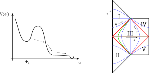
Figure 1: Left panel: The potential for the field $\Phi$. The local minimum at $\Phi=\Phi_{A}$ is the false vacuum, whose geometry is de Sitter space (the ancestor vacuum). On the true vacuum side, it is assumed that a plateau region exists, on which slow-roll inflation occurs. The true minimum of the potential is taken to be zero, since we expect the present cosmological constant to be realized as the vacuum energy of a quantum field on this background. Right panel: Penrose diagram for the Coleman-De Luccia geometry. The spacetime is divided into five regions by the red lines. Region I is an open FLRW universe. The green line represents the bubble wall. On its left (right) is the true (ancestor) vacuum. The blue curves indicate orbits of the $SO(3,1)$ symmetry. The directions of the coordinates ($\eta$, $R$ for Region I; $\tau$, $X$ for Region III) are indicated by arrows. Region I is drawn with the future null infinity, because the present cosmological constant will relax to zero in the future if it is due to the vacuum energy of a quantum field.

The Penrose diagram in Fig. 1, which has null future infinity in Region I, is for the case of the zero final cosmological constant (c.c.). We do not know whether the present c.c. (dark energy) persists into the infinite future. If dark energy is due to the vacuum energy of a quantum field as proposed later in this paper, it will relax to zero in the future, thus we draw the Penrose diagram for this case. If the final c.c. is positive, the 45 degree line for the null infinity is replaced by a more horizontal curve which represents spacelike infinity.

The whole geometry and the configuration of the field $\Phi$ have the $SO(3,1)$ symmetry. The surfaces of constant $\Phi$ are the slices on which the $SO(3,1)$ symmetry acts as isometries. In Region III, these surfaces are timelike, and are (2+1) dimensional de Sitter spaces. In particular, the world volume of the bubble has this symmetry. The bubble wall is the “vacuum domain wall”, which has no structure, and is invariant under the Lorentz boost. On the other hand, in Region I the $SO(3,1)$ symmetric surfaces are spacelike, $H^{3}$. In the thin-wall limit with the zero c.c., Region I is nothing but part of Minkowski space in the open slicing (known as the Milne universe).

2.2 Euclidean metric and its analytic continuation

The geometry containing one bubble of the true vacuum is obtained by analytic continuation from the Euclidean geometry (Coleman-De Luccia [CDL] instanton), which is believed to contribute dominantly to the path integral of quantum gravity.

Let us first describe the Euclidean geometry. The Euclidean version of the 3+1 dimensional de Sitter space is a sphere $S^{4}$, while the CDL instanton is a deformed sphere described by the metric of the following form,

$$ds_{E}^{2}=a^{2}(X)\left(dX^{2}+d\theta^{2}+\sin^{2}\theta d\Omega_{2}^{2}\right).$$ (2.1)

This geometry is topologically $S^{4}$, but is deformed in the $X$ direction. It has an $S^{3}$ factor parametrized by $\theta$ and $\Omega_{2}$, so it preserves the $SO(4)$ subgroup of $SO(5)$. The scale factor $a(X)$ behaves as $a(X)=c_{\pm}e^{\pm X}$ with some constant $c_{\pm}$ for $X\to\mp\infty$ due to the fact that the geometry is smooth (i.e., locally flat) at both ends. We will mostly consider the case where the true vacuum has zero c.c., since this is sufficient for the study of the early time limit in the open FLRW universe (as explained below). In the thin-wall limit for the true vacuum with a zero c.c., the geometry is $S^{4}$ patched with a flat disk at the domain wall located at $X=X_{0}$, and the scale factor takes the form,

$$a(X) =H_{A}^{-1}{e^{X-X_{0}}\over\cosh X_{0}}\quad(X\leq X_{0}),$$

$$={H_{A}^{-1}\over\cosh X}\quad(X_{0}\leq X).$$ (2.2)

The natural length scale associated with this scale factor is the inverse Hubble parameter $H_{A}^{-1}$ of the ancestor vacuum.

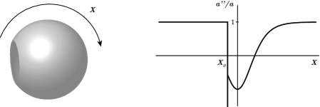
Figure 2: Left panel: The Euclidean geometry for a CDL instanton in the thin-wall limit. A flat space for the true vacuum (whose vacuum energy is assumed to be zero) is patched to a piece of a sphere $S^{4}$ for the false vacuum with a positive vacuum energy. The $S^{3}$ part is represented by $S^{1}$ in the figure. Right panel: The potential $a^{\prime\prime}/a$ in the massless scalar equation of motion (3.3) on a CDL background in the thin-wall limit. Asymptotically, $a^{\prime\prime}/a\to 1$ for $X\to\pm\infty$. On the true-vacuum side ($X<X_{0}$), the potential is flat. At the bubble wall ($X=X_{0}$), there is a negative delta function. If mass is non-zero, the potential will be lifted by the additional term $+m^{2}a^{2}$.

We can analytically continue the geometry from the reflection symmetric surface, namely an equator of the $S^{3}$. With

$$\theta\to i\tau+{\pi\over 2},$$ (2.3)

we obtain the metric covering Region III in Fig. 1,

$$ds^{2}=a^{2}(X)\left(dX^{2}-d\tau^{2}+\cosh^{2}\tau d\Omega_{2}^{2}\right).$$ (2.4)

This has a factor of $(2+1)$-dimensional de Sitter space, parametrized by $\tau$ and $\Omega_{2}$. The $SO(4)$ symmetry of the Euclidean space becomes $SO(3,1)$ after analytic continuation. This symmetry acts as the isometry group of the (2+1) dimensional de Sitter space. The coordinate $X$ parametrizes the spatial direction transverse to these de Sitter spaces. The $X$-direction for $\tau=0$ is represented by the horizontal line in Fig. 1.

Region III is not geodesically complete. The spacetime can be extended past the horizons ($X\to\pm\infty$, $\tau\to\pm\infty$), represented by the 45 degree red lines in Fig. 1, which are locally equivalent to the Rindler horizon. By continuing past $X\to-\infty$, $\tau\to+\infty$, we obtain an open FLRW universe (Region I) described by the metric

$$ds^{2}=a^{2}(\eta)\left(-d\eta^{2}+dR^{2}+\sinh^{2}Rd\Omega_{2}^{2}\right).$$ (2.5)

The spatial sections are $H^{3}$, parametrized by $R$ and $\Omega_{2}$ with the isometry group $SO(3,1)$. This metric (2.5) is most easily obtained by an analytic continuation,

$$X\to\eta+{\pi\over 2}i,\quad\theta\to iR,$$ (2.6)

from the Euclidean metric (2.1). The scale factor behaves as

$$a(\eta)\sim e^{\eta}$$ (2.7)

in the early-time limit $\eta\to-\infty$. In the thin-wall limit with the zero final c.c., the scale factor is exactly $a(\eta)=const.\times e^{\eta}$.

One way to understand the relation between the coordinates in (2.4) and (2.5) is to note that the geometry near the light cone is locally flat. One can use the coordinates $\hat{t}$, $\hat{r}$ to cover the global Minkowski space, $ds_{\rm flat}^{2}=-d\hat{t}^{2}+d\hat{r}^{2}+\hat{r}^{2}d\Omega_{2}^{2}$. The metric (2.4) with $a(X)=e^{X}$ is obtained by

$$\hat{t}=e^{X}\sinh\tau,\quad\hat{r}=e^{X}\cosh\tau,$$ (2.8)

whereas the metric (2.5) with $a(\eta)=e^{\eta}$ is obtained by

$$\hat{t}=e^{\eta}\cosh R,\quad\hat{r}=e^{\eta}\sinh R.$$ (2.9)

2.3 The open FLRW universe

The open FLRW universe (Region I) is entirely inside the bubble, and the CDL instanton sets its initial condition. The scale factor has to behave as $\eqref{aeta}$ in the early-time limit. The evolution afterwards can be found by solving the Friedmann equation,

$${(a^{\prime})^{2}\over a^{4}}={1\over 3M_{P}^{2}}\rho+{1\over a^{2}},$$ (2.10)

where the prime denotes the derivative with respect to the conformal time $\eta$, and $M_{P}$ is the reduced Planck scale. The last term in (2.10) is the contribution from the negative spatial curvature. The energy density $\rho$ and pressure $p$ satisfy the conservation equation,

$$\rho^{\prime}+3{a^{\prime}\over a}(\rho+p)=0.$$ (2.11)

If the energy density of the universe is dominated by that of a classical scalar field $\Phi(\eta)$ which depends only on time, we have

$$\rho={1\over 2a^{2}}(\Phi^{\prime})^{2}+V(\Phi),\quad p={1\over 2a^{2}}(\Phi^{\prime})^{2}-V(\Phi).$$ (2.12)

Just after the beginning of the FLRW time, there is a curvature dominated era in which the scale factor is approximately (2.7). (The spacetime curvature is zero in the early-time limit, and the universe is dominated by the spatial curvature.) This era will continue until the vacuum energy for inflation $\rho=V_{I}$ starts to dominate over the contribution from the curvature $V_{I}\sim M_{P}^{2}/a^{2}$. The consequences of this curvature dominated era have been discussed in detail in [19].

Then, slow-roll inflation occurs. For simplicity, we ignore the gradient of the potential in the plateau region in Fig. 1, and assume that there is a constant energy density $\rho=V_{I}\equiv 3M_{p}^{2}H_{I}^{2}$ from the beginning of the FLRW time until the end of slow-roll inflation. We will also ignore a possible fast-rolling phase after tunneling and before slow-roll inflation. We expect these features will give only small corrections to our main result.

The solution of (2.10) with $\rho=3M_{p}^{2}H_{I}^{2}$ is

$$a(\eta)={H_{I}^{-1}\over\sinh(-\eta)},$$ (2.13)

up to a shift of $\eta$. We could replace $\eta$ in (2.13) by $\eta-\tilde{\eta}_{1}$ where

$$e^{\tilde{\eta}_{1}}={H_{A}\over H_{I}}~{}(1+e^{2X_{0}}),$$ (2.14)

so that (2.13) becomes $a(\eta)=H_{A}^{-1}e^{\eta-X_{0}}/\cosh X_{0}$ in the early-time limit $\eta\to-\infty$, to match the normalization of the Euclidean scale factor (2.2), but we will not do this in the following. Instead, we will use (2.13) in the FLRW universe, and replace $\eta$ by $\eta+\tilde{\eta}_{1}$ in the correlators obtained by analytic continuation from the Euclidean space. See eq. (4.4) below.

After the slow-roll inflation, reheating occurs, and the radiation and matter dominated eras will follow. The evolution through these eras until the present time will be studied in Section 5.

3 Correlation functions

We now start to calculate the two-point functions in the early-time limit in the FLRW universe. We will first find the correlator in the Euclidean space (2.1), and analytically continue it to the Lorentzian spacetime. The essential part of the calculation is the decomposition of the field into a complete set of states in the $X$ direction (along the horizontal line in Fig. 1). For more details of this calculation, see Appendix of [26].

3.1 Calculation in Euclidean space

We consider the Euclidean CDL geometry, and compute correlation functions of a minimally coupled scalar field $\phi$, which is described by the action

$$S=\int d^{4}x\sqrt{g}~{}\frac{1}{2}\left(g^{\mu\nu}\partial_{\mu}\phi\partial_{\nu}\phi+m^{2}\phi^{2}\right).$$ (3.1)

The field $\phi$ is different from the tunneling field $\Phi$. We assume $\phi$ to have the zero expectation value, and can be treated as a free field on the curved (CDL) background. It is convenient to define a field $\chi(X,\Omega_{3})=a(X)\phi(X,\Omega_{3})$, for which the kinetic term is independent of $a(X)$, $S=\int dXd\Omega_{3}(\partial_{X}\chi)^{2}+\cdots$.

We would like to obtain the two-point function that satisfies the equation of motion with a delta-function source,

$$\left[-\partial_{X}^{2}+{a^{\prime\prime}(X)\over a(X)}+m^{2}a^{2}(X)-\nabla_{S}^{2}\right]\langle\chi(X,\Omega_{3})\chi(X^{\prime},0)\rangle=\delta(X-X^{\prime})\delta^{3}(\Omega_{3}),$$ (3.2)

where $\nabla_{S}^{2}$ and $\delta^{3}(\Omega_{3})$ are the Laplacian and delta function, respectively, on $S^{3}$.

We will obtain the correlator as an expansion in the complete basis in the $X$ direction. In the Lorentzian geometry, the $X$ direction lies along a global Cauchy surface (See Fig. 1). The complete basis is formed by the eigenfunctions $u^{I}_{k}(X)$ of the following differential operator,

$$\left[-\partial_{X}^{2}+{a^{\prime\prime}(X)\over a(X)}+m^{2}a^{2}(X)\right]u^{I}_{k}(X)=(k^{2}+1)u^{I}_{k}(X),$$ (3.3)

where $k$ labels the eigenvalue, and $I$ is either $L$ ($R$) for waves coming from the left (right), or $B$ for the bound state. This equation is of the form of the time-independent Schrödinger equation in one dimension. The potential $a^{\prime\prime}/a+m^{2}a^{2}$ approaches $+1$ for $X\to\pm\infty$ (see Fig 2). Thus, the modes for real $k(>0)$ with the eigen-energy larger than $+1$ are the waves oscillating in $X$. The orthogonal set consists of the waves coming from the left $u_{k}^{L}(X)$, and those from the right $u_{k}^{R}(X)$, which satisfy

$$u^{L}_{k}(X) \to e^{ikX}+{\cal R}(k)e^{-ikX}\quad(X\to-\infty),$$

$$\to{\cal T}(k)e^{ikX}\quad(X\to\infty),$$ (3.4)

and

$$u^{R}_{k}(X) \to{\cal T}_{R}(k)e^{-ikX}\quad(X\to-\infty),$$

$$\to e^{-ikX}+{\cal R}_{R}(k)e^{ikX}\quad(X\to\infty).$$ (3.5)

${\cal R}(k)$ and ${\cal T}(k)$ are the reflection and transmission coefficients for the scattering from the left, and ${\cal R}_{R}(k)$ and ${\cal T}_{R}(k)$ are those for the scattering from the right. They are related by ${\cal T}(k)={\cal T}_{R}(k)$, ${\cal R}(k)/{\cal R}_{R}(k)^{*}=-{\cal T}(k)/{\cal T}(k)^{*}$. For negative real $k$, we define ${\cal R}(-k)={\cal R}^{*}(k)$, ${\cal T}(-k)={\cal T}^{*}(k)$. From the conservation of the probability current, we have ${\cal R}(k){\cal R}^{*}(k)+{\cal T}(k){\cal T}^{*}(k)=1$. (See e.g., [44] for basic facts about the scattering problem in one dimension.) These modes satisfy the orthogonality property

$$\int_{-\infty}^{\infty}dXu^{I}_{k}(X)u^{*J}_{k^{\prime}}(X)=2\pi\delta^{IJ}\delta(k-k^{\prime}),$$ (3.6)

where $I,J$ are either $L$ or $R$.

If there are bound states in (3.3), one has to include them in the complete set. Bound states occur at discrete imaginary values of the momentum $k=k_{B}$ with ${\rm Im}(k_{B})>0$. At $k=k_{B}$, both ${\cal R}(k_{B})$ and ${\cal T}(k_{B})$ have a pole. This means that $e^{\pm ik_{B}X}$ in $u^{L/R}_{k}(X)$ is negligible compared to ${\cal R}(k_{B})e^{\mp ik_{B}X}$ and ${\cal T}(k_{B})e^{\pm ik_{B}X}$, thus the wave function (3.4) with $k=k_{B}$ decays at both ends $X\to\pm\infty$, and is normalizable.

Let us first consider the massless case. In this case, one can easily see that

$$u^{B}_{k=i}(X)={\cal N}H_{A}a(X)$$ (3.7)

satisfies (3.3) with $k=i$ where ${\cal N}$ is a dimensionless constant. An example of the potential ${a^{\prime\prime}/a}$ for the Schrödinger equation (3.3) is depicted in Fig. 2. The bound state is essentially supported at the dip of the potential. If the geometry is compact in the $X$ direction (which is the case for de Sitter space or the CDL geometry, but not for anti-de Sitter space or Minkowski space), this mode is normalizable and should be included in the complete set. It can be shown that there is at most one bound state in 3+1 dimensions [17, 26]. Normalization factor ${\cal N}$ in the thin-wall limit (2.2) is

$${\cal N}^{-2} =\int^{\infty}_{-\infty}dX(H_{A}a)^{2}(X)=\int_{-\infty}^{X_{0}}dX\left({e^{X-X_{0}}\over\cosh X_{0}}\right)^{2}+\int_{X_{0}}^{\infty}dX{1\over\cosh^{2}X}$$ (3.8)

$$={1\over 2\cosh^{2}X_{0}}+1-\tanh X_{0}.$$ (3.9)

In the limit of $X_{0}\to-\infty$ (the limit of the small bubble), we get a finite value ${\cal N}\to 1/\sqrt{2}$, which agrees with the case for the pure de Sitter.

When the scalar field has mass, the additional term $+m^{2}a^{2}(X)$ lifts the potential, and the dip in the potential becomes shallow. The energy of the bound state (as long as exists) increases, shifting the pole from $k_{B}=i$ in the massless case to

$$k_{B}=i(1-\epsilon).$$ (3.10)

If mass is larger than a certain value (which is of order $H_{A}$), the bound state disappears.

We will consider the possibility that mass of the field $\phi$ is different in the true and the false vacuum,

$$m=\left\{\begin{array}[]{ll}m_{A}&\qquad(\mbox{False vacuum})\\ m_{0}&\qquad(\mbox{True vacuum})\\ \end{array}\right.\ ,$$ (3.11)

where $m_{A}$ and $m_{0}$ are assumed to be constant. The case of our interest is $m_{A}\ll H_{A}$ and $m_{0}\sim H_{0}\ll m_{A}$. In this case we can set $m_{0}=0$ in the analysis of the early-time behavior performed in this section, since such a tiny $m_{0}$ as compared to the natural scale (the Hubble parameter at the time in question) will not affect the dynamics.

It is not easy to calculate $\epsilon$ (i.e., the bound state energy) in general, but when $m_{A}H_{A}^{-1}$ is small, as in the case of our interest, it can be evaluated by the first-order perturbation theory. We take (3.7) as the zeroth-order wave function and $m^{2}a^{2}(X)$ as perturbation Hamiltonian in the one-dimensional Schrödinger-like equation  (3.3). The eigen-energy $E=(k_{B}^{2}+1)=1-(1-\epsilon)^{2}$ is zero at the zeroth order. The first-order eigen-energy, $E^{(1)}=2\epsilon$, is

$$E^{(1)}=\int_{-\infty}^{\infty}dX\left(\psi^{(0)}(X)\right)^{2}m^{2}a^{2}(X).$$ (3.12)

with the zeroth-order (massless) wave function,

$$\psi^{(0)}(X)={\cal N}H_{A}a(X).$$ (3.13)

Thus, for the case of $m_{0}^{2}=0$, we obtain

$$\epsilon ={{\cal N}^{2}\over 2}m_{A}^{2}H_{A}^{-2}\int_{X_{0}}^{\infty}dX{1\over\cosh^{4}X}$$

$$={{\cal N}^{2}\over 2}\left({2\over 3}-{1\over 3}\left(2+{\rm sech}^{2}X_{0}\right)\tanh X_{0}\right)m_{A}^{2}H_{A}^{-2}$$

$$={2-(2+{\rm sech}^{2}X_{0})\tanh X_{0}\over 3\,(2+{\rm sech}^{2}X_{0}-2\tanh X_{0})}m_{A}^{2}H_{A}^{-2}.$$ (3.14)

The reflection coefficient ${\cal R}(k)$ for (3.3) with $m_{A}=m_{0}=0$ in the thin-wall limit (2.1) can be obtained exactly [26],

$${\cal R}(k)={\gamma ie^{2ikX_{0}}\over(k+\gamma i)}{(k+i)\over(k-i)},$$ (3.15)

where $\gamma$ is given by

$$\gamma={1\over 1+e^{-2X_{0}}},$$ (3.16)

and takes a value $0<\gamma<1$. The $k=i$ pole corresponds to the bound state. The pole in the lower half plane ($k=-i\gamma$) does not correspond to a physical mode for (3.3), since the wave function blows up at $X\to\pm\infty$ and is not normalizable.

Using this complete set, the correlation function satisfying (3.2) can be expressed as

$$\langle\chi(X,\theta)\chi(X^{\prime},0)\rangle =\int_{0}^{\infty}{dk\over 2\pi}\left(u^{L}_{k}(X)u^{L*}_{k}(X^{\prime})+u^{R}_{k}(X)u^{R*}_{k}(X^{\prime})\right)G_{k}(\theta)$$

$$+u^{B}_{k}(X)u^{B*}_{k}(X^{\prime})G_{k}(\theta),$$ (3.17)

where $G_{k}(\theta)$ is the Green’s function on $S^{3}$ for a field with the effective mass $(k^{2}+1)$,

$$\left[-\nabla_{S}^{2}+(k^{2}+1)\right]G_{k}(\theta)={\delta(\theta)\over 4\pi\sin^{2}\theta}.$$ (3.18)

$G_{k}(\theta)$ is a function of the geodesic distance $\theta$ on $S^{3}$, and given by

$$G_{k}(\theta)={\sinh k(\pi-\theta)\over 4\pi\sinh k\pi\sin\theta}.$$ (3.19)

We can see that $G_{k}(\theta)$ is the correct Green’s function on $S^{3}$ by noting the following facts. $G_{k}(\theta)$ satisfies the Laplace equation, and is regular everywhere on $S^{3}$ except for the source $\theta=0$ with the correct singularity $G_{k}(\theta)\sim 1/(4\pi\theta)$ at $\theta=0$.

There is a subtlety when the mass of the scalar field $\phi$ is exactly zero. We have a bound state with $k=i$, and the effective mass on $S^{3}$ becomes zero, $k^{2}+1=0$. But there does not exist such a Green’s function on a compact space, since the flux cannot extend to infinity and the Gauss law cannot be satisfied. (In other words, the differential operator in the equation of motion cannot be inverted in this case, since the equation is unchanged under the constant shift of $\phi$). See [26] for how to deal with this case. In this paper, we will not have this problem, since we will always consider the massive field.

The correlation function in the $X\to-\infty$ limit (i.e., on the true vacuum side) when $m_{0}=0$, can be written as

$$\langle\chi(X,\theta)\chi(X^{\prime},0)\rangle=\int_{{\cal C}_{1}}{dk\over 8\pi^{2}}\left(e^{ik(X-X^{\prime})}+{\cal R}(k)e^{-ik(X+X^{\prime})}\right){\sinh k(\pi-\theta)\over\sinh k\pi\sin\theta}.$$ (3.20)

If we take the thin-wall limit, (3.20) is valid throughout the $X<X_{0}$ region. The integration contour ${\cal C}_{1}$ is defined in Fig. 3. This contour is basically along the real axis but is deformed near the origin so that it goes above the bound state pole. This deformation amounts to adding a discrete mode due to the bound state.

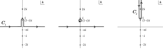
Figure 3: Left panel: The definition of the contour ${\cal C}_{1}$ for the $k$-integration. Middle panel: A contour equivalent to ${\cal C}_{1}$. The residue at the $k=(1-\epsilon)i$ pole is equal to the bound state contribution (the second line) in (3.17). Right panel: The contour ${\cal C}_{2}$ used at the end of Section 4 to show the finiteness of $\langle\phi^{2}\rangle$ in the early-time ($\eta,\eta^{\prime}\to-\infty$) limit. By deforming ${\cal C}_{1}$ to ${\cal C}_{2}$, the $k$-integral is expressed as a sum over the residues at $k=in$ ($n=1,2,\ldots$).

Note that the normalization factor $1/\sinh k\pi$ for the $S^{3}$ Green’s function $G_{k}(\theta)$ introduces poles at integer multiple of $k=i$. Thus, if the mass is exactly zero, the pole at $k=i$ becomes a double pole. As mentioned above, we will always consider the massive case, so the contour ${\cal C}_{1}$ passes between $k=i(1-\epsilon)$ and $k=i$. We can take the massless limit starting from this expression, if necessary.

3.2 Analytic continuation to Lorentzian

We perform the analytic continuation (2.6) on (3.20), and obtain the correlation function in the FLRW universe,

$$\langle\chi(\eta,R)\chi(\eta^{\prime},0)\rangle =\int_{-\infty}^{\infty}{dk\over 8\pi^{2}}e^{ik(\eta-\eta^{\prime})}{\sinh k(\pi-iR)\over i\sinh k\pi\sinh R}$$

$$+\int_{{\cal C}_{1}}{dk\over 8\pi^{2}}{\cal R}(k)e^{-ik(\eta+\eta^{\prime})}{\sin kR\over\sinh k\pi\sinh R}.$$ (3.21)

This is valid in the early-time limit $\eta,\eta^{\prime}\to-\infty$ (i.e., the curvature dominated era), and can be regarded as the initial condition for the correlator in the FLRW universe. The correlator at later times will be obtained in Section 5.

A subtle prescription for analytic continuation has been used to obtain the second term in (3.21). If we naively made the substitution (2.6) in the second term in (3.20), we would have gotten

$$e^{-ik(X+X^{\prime})}\,{\sinh k(\pi-\theta)\over\sinh k\pi}\to e^{-ik(\eta+\eta^{\prime})}\,{\left(e^{2k\pi-ikR}-e^{ikR}\right)\over 2\sinh k\pi},$$ (3.22)

but the first term in the numerator on the right hand side of (3.22) diverges for $k\to\infty$, so the $k$ integral along the real axis does not converge. To get a convergent integral, we should make a replacement

$$\sinh k(\pi-\theta)\to e^{-k\pi}\sinh\theta$$ (3.23)

in (3.20) before the analytic continuation. This is allowed, since the replacement (3.23) does not change the result of the integration in (3.20). The integral can be evaluated by deforming the contour and summing up the residues of the poles at $k=ni$ with $n=1,2,\ldots$. As a result, multiplication by $e^{2k\pi}$ amounts to multiplication of each residue by unity, so the answer does not change. By performing analytic continuation after the replacement (3.23), we obtain the second term in (3.21). On the other hand, for the first term in (3.20), analytic continuation should be done using the original expression. The $k$-integral converges with this integrand, but does not converge if we make the replacement (3.23).

In fact, evaluating the integral (3.20) as sum over the poles at $k=ni$ ($n=1,2,\ldots$) is equivalent to expanding the correlator into spherical harmonics on $S^{3}$. Total angular momentum $L$ on $S^{3}$ is related to the position of the pole by $L=n-1$. For the calculation of the correlator starting from this representation of discrete sum, and using Watson-Sommerfeld transformation to convert it into an integral, see e.g., [45, 46].

The correlator (3.21) is a function of the geodesic distance $R$ on $H^{3}$. In other words, one point is set at the origin and the other point is at a radial distance $R$ from the origin. When two points are at general positions on $H^{3}$, we can rewrite the correlator using the relation

$$\cosh R=\cosh R_{1}\cosh R_{2}-\sinh R_{1}\sinh R_{2}\cos\psi.$$ (3.24)

where $R_{1}$ and $R_{2}$ are the radial coordinates of the two points, and $\psi$ is the angle on $S^{2}$ between them.

The correlator can also be expressed as a sum over products of harmonics $f^{(\ell,m)}_{k}(R,\Omega_{2})$ at the two points. Harmonics on $H^{3}$ are the eigenfunctions of Laplacian,

$$\nabla_{H}^{2}f^{(\ell,m)}_{k}(R,\Omega_{2})=-(k^{2}+1)f^{(\ell,m)}_{k}(R,\Omega_{2}).$$ (3.25)

The modes with real $k$ are normalizable on $H^{3}$,

$$\int_{0}^{\infty}dR\sinh^{2}R\int d\Omega_{2}f^{(\ell,m)}_{k}(R,\Omega_{2})f^{(\ell^{\prime},m^{\prime})*}_{k^{\prime}}(R,\Omega_{2})=\delta(k-k^{\prime})\delta_{\ell,\ell^{\prime}}\delta_{m,m^{\prime}}.$$ (3.26)

The $\ell=0$ mode, which is homogeneous on $S^{2}$, is a function of only the radial coordinate,

$$f^{(\ell=0)}_{k}(R)=\frac{1}{\sqrt{2}\pi}{\sin kR\over\sinh R}\ .$$ (3.27)

When one point is at the origin $R_{1}=0$ or $R_{2}=0$, only the $\ell=0$ mode contributes to the two-point functions (as is familiar in the harmonic expansion in quantum mechanics in flat space). The factor $\sinh R$ in the denominator of (3.27) compensates for the exponential growth of the volume for large $R$ on the hyperboloid. For the explicit form of the harmonics with $\ell\neq 0$, see Appendix A and [11, 12, 13].

Note that a constant function on $H^{3}$ is not normalizable. To express non-normalizable functions, which decay more slowly than $e^{-R}$ as $R\to\infty$ (with arbitrary dependence on $S^{2}$), we need the modes with imaginary $k$. As indicated by the integration contour ${\cal C}_{1}$, the correlator (3.21) contains a discrete non-normalizable mode on $H^{3}$, which is called the “supercurvature mode” [11, 12, 13]. As we have seen, a bound state in the Euclidean problem is in one-to-one correspondence with a supercurvature mode on $H^{3}$.

The first term in (3.21), which is a function of $\eta-\eta^{\prime}$, is nothing but the correlator in global Minkowski space written in the open slicing. This can be seen by rewriting the massless correlator in terms of Minkowski coordinates $\hat{t}$, $\hat{r}$, and performing the coordinate transformation (2.9),

$$\langle\phi(\eta,R)\phi(\eta^{\prime},0)\rangle ={1\over\left(-(\hat{t}-\hat{t^{\prime}})^{2}+\hat{r}^{2}\right)}$$

$$={1\over 2e^{\eta+\eta^{\prime}}\left(\cosh R-\cosh(\eta-\eta^{\prime})\right)},$$ (3.28)

where we have put one point at the origin $\hat{r}^{\prime}=0$. Carrying out the $k$ integral for the first term in (3.21) as a sum over the residues from the poles, we recover the r.h.s. of (3.28).

The second term, which is a function on $\eta+\eta^{\prime}$ and depends on the reflection coefficient ${\cal R}(k)$, carries the information about the ancestor vacuum. This term is finite in the coincident-point limit $R\to 0$, $\eta-\eta^{\prime}\to 0$.

4 Energy-momentum tensor

We now compute the contribution of a quantum field to the energy-momentum tensor, by taking the coincident-point limit of the two-point function obtained in the previous section.

4.1 General remarks

The energy-momentum tensor for a minimally coupled scalar field is

$$T_{\mu\nu}=\partial_{\mu}\phi\partial_{\nu}\phi-{1\over 2}g_{\mu\nu}\left(\partial^{\rho}\phi\partial_{\rho}\phi+m^{2}\phi^{2}\right).$$ (4.1)

The energy density $\rho=-\langle T^{\eta}_{~{}\eta}\rangle$ and pressure $p=\langle T^{i}_{~{}i}\rangle$, where $i$’s are not summed over, are obtained by taking the vacuum expectation value of (4.1):

$$\rho = \frac{1}{a^{2}}\left\langle\frac{1}{2}\phi^{\prime 2}+\frac{1}{2}(\nabla\phi)^{2}+\frac{1}{2}m^{2}a^{2}\phi^{2}\right\rangle\ ,$$ (4.2)

$$p = \frac{1}{a^{2}}\left\langle\frac{1}{2}\phi^{\prime 2}-\frac{1}{6}(\nabla\phi)^{2}-\frac{1}{2}m^{2}a^{2}\phi^{2}\right\rangle\ .$$ (4.3)

They can be computed from the two-point function in the the coincident-point limit.

The two-point function (3.21) consists of two terms. The first term is independent of the ancestor vacuum. In the early-time limit, it coincides with the correlator in the global Minkowski space. We will touch on this term only briefly in this paper, since the analysis of this term is essentially contained in the previous work [28, 29].

The second term in (3.21) depends on the properties of the ancestor vacuum. The supercurvature mode is involved in this term. We will mostly focus on this second term, which is larger than the first term in the cases of interest, as we will see later. The value of the second term is found to be finite in the coincident-point limit, and thus is independent of the renormalization prescription for the UV divergence.

The wave functions in the ancestor vacuum are of order $H_{A}$, the natural mass scale in de Sitter space. As we will see in detail in Section 5, the continuous modes have the time dependence $e^{-\eta}$, and they decreases to order $H_{I}$, which is the natural magnitude of fluctuations in slow-roll inflation with the Hubble parameter $H_{I}$, by the end of the curvature domination [19]. The supercurvature mode has the time dependence $e^{-\epsilon\eta}$, and decays more slowly than the continuous modes. Furthermore, its contribution to $\langle\phi^{2}\rangle$ is enhanced by an extra factor $\epsilon^{-1}\sim H_{A}^{2}/m_{A}^{2}$, as we will see shortly.

The continuous modes are different from the modes in the flat FLRW cosmology, in the sense that the infrared modes are cut off by the spatial curvature. We can see this e.g., in (3.27) where the mode with real $k$ decays exponentially for $R\gtrsim 1$.

4.2 Mass term in the limit of small mass

Let us study the mass term in the limit of small mass ($\epsilon$), which will be the most dominant term in the energy density of the scalar field.

The correlation function in the early time limit $\eta,\eta^{\prime}\to-\infty$ is

$$\langle\chi(\eta,R)\chi(\eta^{\prime},0)\rangle =\int_{-\infty}^{\infty}{dk\over 8\pi^{2}}e^{ik(\eta-\eta^{\prime})}{\sinh k(\pi-iR)\over i\sinh k\pi\sinh R}$$

$$+\int_{{\cal C}_{1}}{dk\over 8\pi^{2}}{\cal R}(k)e^{-ik(\eta+\eta^{\prime}+2\tilde{\eta}_{1})}{\sin kR\over\sinh k\pi\sinh R},$$ (4.4)

where we have made the shift $\eta\to\eta+\tilde{\eta}_{1}$ with $\tilde{\eta}_{1}$ defined in (2.14) (similarly for $\eta^{\prime}$) in (3.21), to account for the difference in the definition of $\eta$ mentioned in Section 2.

The contribution from the $k=i(1-\epsilon)$ pole is

$$\langle\chi(\eta,R)\chi(\eta^{\prime},0)\rangle^{\rm(s.c.m.)}={(-2\pi i)\over 8\pi^{2}}\cdot\mbox{Res}(i(1-\epsilon))e^{(1-\epsilon)(\eta+\eta^{\prime}+2\tilde{\eta}_{1})}{1\over\sin\epsilon\pi}{\sinh(1-\epsilon)R\over\sinh R},$$ (4.5)

where $\mbox{Res}(i(1-\epsilon))$ denotes the residue of $R(k)$ at $k=i(1-\epsilon)$. This gives the contribution from the supercurvature mode on $H^{3}$. Dividing (4.5) by $a(\eta)a(\eta^{\prime})$, and taking the coincident-point limit $\eta\to\eta^{\prime}$, $R\to 0$, we obtain the expectation value $\langle\phi^{2}(\eta)\rangle^{\rm(s.c.m.)}$.

Let us explicitly evaluate $\langle\phi^{2}(\eta)\rangle^{\rm(s.c.m.)}$ in the $\epsilon\to 0$ limit. In this limit, one can use the residue of $R(k)$ for $\epsilon=0$, given by (3.15), and obtain

$$\langle\phi^{2}(\eta)\rangle^{\rm(s.c.m.)}={1\over 4\pi^{2}\epsilon}A(X_{0})e^{-2\epsilon(\eta+\tilde{\eta}_{1})}H_{A}^{2}\ ,$$ (4.6)

where $A(X_{0})$ depends on $X_{0}$ (i.e., the size of the bubble),

$$A(X_{0})={(1+e^{2X_{0}})^{2}\over 2(1+2e^{2X_{0}})}.$$ (4.7)

We have kept $\epsilon$ in the denominator and in the time-dependent function $e^{-2\epsilon(\eta+\tilde{\eta}_{1})}$, but have replaced the term $e^{2(1-\epsilon)X_{0}}$ by $e^{2X_{0}}$, since this difference will not have a large effect. Using the value of $\epsilon$ obtained by the first-order perturbation theory in (3.14), the expectation value (4.6) becomes

$$\langle\phi^{2}(\eta)\rangle^{\rm(s.c.m.)}={1\over 2\pi^{2}}\cdot{3\,e^{-2\epsilon(\eta+\tilde{\eta}_{1})}\over 2-(2+{\rm sech}^{2}X_{0})\tanh X_{0}}\cdot{H_{A}^{4}\over m_{A}^{2}}.$$ (4.8)

In the limit of the small bubble $X_{0}\to-\infty$, (and $\epsilon\to 0$), (4.8) approaches ${3\over 8\pi^{2}}{H_{A}^{4}\over m_{A}^{2}}$. This agrees with the well-known result in pure de Sitter space obtained by the standard techniques (see e.g., [35, 36]). For the convenience of the reader, we summarize the calculation of $\langle\phi^{2}\rangle$ for the pure de Sitter case in Appendix B.

One may worry that $\langle\phi^{2}(\eta)\rangle^{\rm(s.c.m.)}$ given in (4.6) or (4.8) diverges in the early-time limit $\eta\to-\infty$. In fact, the full expression $\langle\phi^{2}(\eta)\rangle$ also including the continuous modes is regular, as can be shown by deforming the contour for the $k$-integration: At early times, the $e^{-ik(\eta+\eta^{\prime})}$ factor in $\langle\chi(\eta)\chi(\eta^{\prime})\rangle$ gives a converging factor for ${\rm Im}(k)>0$, allowing us to deform the contour ${\cal C}_{1}$ into ${\cal C}_{2}$ defined on the right panel in Fig. 3. Then the $k$-integral is represented as a sum over the residues at the poles at $k=in$ $(n=1,2,\ldots)$. The time-dependence of each residue in $\langle\chi(\eta)\chi(\eta^{\prime})\rangle$ is given by $e^{-ik(\eta+\eta^{\prime})}=e^{n(\eta+\eta^{\prime})}$. The leading term in the early-time limit comes from $n=1$, giving $\langle\phi^{2}(\eta)\rangle=\langle\chi^{2}(\eta)\rangle/a^{2}(\eta)\sim{\rm const.}$

5 Evolution of vacuum energy

Having obtained the vacuum expectation value of the energy-momentum tensor in the early-time limit in the FLRW universe, we now study its time evolution. First, in Section 5.1, we determine the scale factor for the background open universe. Then, in Section 5.2, we obtain the wave function by solving the equation of motion for the scalar field, and in Section 5.3, we study the evolution of the vacuum expectation value of the energy-momentum tensor. Although our analysis is general, we will mostly focus on the supercurvature mode. Finally, in Section 5.4, we consider the possibility that the vacuum energy gives the present dark energy.

5.1 The scale factor

The scale factor for an open universe can be found by solving the Friedmann equation,

$${(a^{\prime})^{2}\over a^{4}}={1\over 3M_{P}^{2}}\rho+{1\over a^{2}},$$ (5.1)

with the energy density $\rho$ appropriate for each era.

The universe at early times is curvature dominated (CD). As we mentioned in section 2.3, when the vacuum energy of inflation dominates over the curvature contribution, the slow-roll inflation occurs. The scale factor in the CD and Inflation eras is given in (2.13). After reheating, the universe becomes radiation dominated (RD). For simplicity, we assume the reheating occurs instantaneously. In fact, the reheating process takes place for producing the particles, mainly of sub-horizon modes, which the inflation field is coupled to. Thus the detailed dynamics of particle production will be irrelevant to our main concern on the energy density given by the supercurvature mode. Then, after the matter-radiation equality, the universe becomes matter dominated (MD).

The scale factors in each era are obtained by solving (5.1) as

$$a(\eta)=\left\{\begin{array}[]{lll}a_{\rm CDInf}(\eta)=-\frac{1}{H_{I}\sinh(\eta)}&(-\infty<\eta<\eta_{1}<0)&(\mbox{CD-Inflation})\\ a_{\rm RD}(\eta)=\alpha\sinh(\eta)&(0<\eta_{2}<\eta<\eta_{3})&(\mbox{RD})\\ a_{\rm MD}(\eta)=\beta\sinh^{2}(\eta/2)&(\eta_{4}<\eta<\eta_{0})&(\mbox{MD})\end{array}\right.$$ (5.2)

with $\rho=3M_{p}^{2}\alpha^{2}/a^{4}$ for the RD era and $\rho=3M_{p}^{2}\beta/a^{3}$ for the MD era.. We will connect them by requiring $a(\eta)$ and $a^{\prime}(\eta)$ are continuous across each era. Here, we closely follow the convention of ref. [28]. Namely, we introduce the different shift of $\eta$ in each era, to keep the expression of $a(\eta)$ simple. The conformal time at present is $\eta=\eta_{0}$. We ignore the present cosmological constant (dark energy) and assume the MD era continues until now.

The continuity conditions for $a$ and $a^{\prime}$ give the following relations among the parameters in (5.2):

$$\eta_{1} = -\eta_{2}\ ,$$ (5.3)

$$\sinh^{2}(\eta_{1}) = \frac{1}{\alpha H_{I}}\ ,$$ (5.4)

$$\eta_{3} = \frac{\eta_{4}}{2}\ ,$$ (5.5)

$$\sinh(\eta_{3}) = \frac{\alpha}{\beta}\ .$$ (5.6)

The Hubble parameter in each era is calculated from (5.2) as

$$H=\frac{a^{\prime}}{a^{2}}=\left\{\begin{array}[]{ll}H_{I}\cosh(\eta)&(\mbox{CD-Inflation})\\ \frac{\cosh(\eta)}{\alpha\sinh^{2}(\eta)}&(\mbox{RD})\\ \frac{\cosh(\eta/2)}{\beta\sinh^{3}(\eta/2)}&(\mbox{MD})\end{array}\right.\ .$$ (5.7)

Comparing the Hubble parameters at the beginning and the end of each era, we obtain a relation

$$\sinh^{2}(\eta_{2})\sinh(\eta_{3})\frac{\cosh(\eta_{0}/2)}{\sinh^{3}(\eta_{0}/2)}=\frac{H_{0}}{H_{I}}\ ,$$ (5.8)

where $H_{0}$ is the present Hubble parameter. This can also be obtained by multiplying (5.4), (5.6), and (5.7) at present time. From observations [9], we know

$$H_{0}\simeq 67{\rm km}~{}{\rm s}^{-1}{\rm Mpc}^{-1}\simeq 1.4\times 10^{-30}{\rm meV}\ ,$$ (5.9)

$$H_{I}\lesssim 3.6\times 10^{-5}M_{P}\simeq 8.8\times 10^{25}{\rm meV}\ ,$$ (5.10)

where meV=$10^{-3}$eV, and $M_{P}=(8\pi G_{N})^{-1/2}\simeq 2.4\times 10^{30}{\rm meV}$ is the (reduced) Planck scale.

The ratio of the curvature radius $R_{c}=a$ (note that curvature radius is unity in the comoving coordinate) to the Hubble radius $H^{-1}=a^{2}/a^{\prime}$ is

$$r_{c}\equiv{R_{c}\over H^{-1}}={a^{\prime}\over a}=\left\{\begin{array}[]{ll}-\coth(\eta)&(\mbox{CD-Inflation})\\ \coth(\eta)&(\mbox{RD})\\ \coth(\eta/2)&(\mbox{MD})\end{array}\right.\ .$$ (5.11)

This ratio grows during inflation, and decreases during the RD and the MD eras. $r_{c}$ is a huge number at the end of inflation, and remains large until now due to the observational bound at present time [9],

$$r_{c0}\gtrsim 10\quad(\mbox{now}).$$ (5.12)

The redshift parameter at the matter-radiation equality is

$$z_{\rm eq}\simeq 3.4\times 10^{3}\ ,$$ (5.13)

and thus we have

$$1+z_{\rm eq}=\frac{a_{0}}{a_{4}}=\frac{\sinh^{2}(\eta_{0}/2)}{\sinh^{2}(\eta_{4}/2)}\ .$$ (5.14)

Using the above relations, we now estimate the values of the parameters $\eta_{1}$, $\eta_{2}$, $\eta_{3}$, $\eta_{4}$, $\eta_{0}$, $\alpha$ and $\beta$ in (5.2). From (5.11) at present and (5.14), the values of $\eta_{0}$ and $\eta_{4}$ are constrained as

$$\eta_{0} \simeq 2r_{c0}^{-1}\lesssim 0.2\ ,$$ (5.15)

$$\frac{\eta_{4}}{\eta_{0}} \simeq z_{\rm eq}^{-1/2}\simeq 1.7\times 10^{-2}\ ,$$ (5.16)

where (5.12) and (5.13) are used. Then, from (5.6), and (5.7) at present, the values of $\alpha$ and $\beta$ are obtained,

$$\frac{\alpha}{\beta} \simeq \frac{\eta_{4}}{2}\simeq r_{c0}^{-1}z_{\rm eq}^{-1/2}\lesssim 2\times 10^{-3}\ ,$$ (5.17)

$$\beta H_{0} \simeq \left(\frac{\eta_{0}}{2}\right)^{-3}\simeq r_{c0}^{3}\gtrsim 1\times 10^{3}\ .$$ (5.18)

Finally, with (5.4), the value of $\eta_{2}$ is estimated as

$$\eta_{2}\simeq\left(\frac{\beta}{\alpha}\frac{1}{\beta H_{0}}\frac{H_{0}}{H_{I}}\right)^{1/2}\simeq r_{c0}^{-1}z_{\rm eq}^{1/4}\left(\frac{H_{0}}{H_{I}}\right)^{1/2}\sim 10^{-28}\ ,$$ (5.19)

where the lower bound for $r_{c0}$ and the upper bound for $H_{I}$ are applied in the last equality.

Slow-roll inflation starts when the inflaton potential starts to dominate over the curvature term, i.e., at $\eta\sim-1$. The e-folds $N_{e}$ of the slow-roll inflation is

$$N_{e}=\log\left(\frac{a_{\rm CDInf}(\eta_{1})}{a_{\rm CDInf}(-1)}\right)\sim 64.6\ ,$$ (5.20)

where we have used (5.19) for the value of $\eta_{1}=-\eta_{2}$. If we take larger values for $r_{c0}$ (the ratio between the curvature radius and Hubble radius at present), $N_{e}$ becomes larger. Since the value (5.20) roughly coincides with the value derived from an anthropic bound for the spatial curvature [19], it would be reasonable to adopt these minimal values for $r_{c0}$ and $N_{e}$.

5.2 Wave functions

5.2.1 Equation of motion

We now consider a minimally coupled scalar field $\phi$ in the open FLRW universe. The equation of motion for $\chi$, which is defined as $\phi=\chi/a$, is

$$\left[-\partial_{\eta}^{2}+{a^{\prime\prime}\over a}+\nabla_{H}^{2}-m_{0}^{2}a^{2}\right]\chi(\eta,{\cal H})=0\ ,$$ (5.21)

where ${\cal H}$ and $\nabla_{H}^{2}$ denote the coordinates and Laplacian, respectively, on $H^{3}$ . The mass term in (5.21) is the mass $m_{0}$ after tunneling.

We expand the field into harmonics on $H^{3}$, defined in (3.25),

$$\chi(\eta,{\cal H})=\int_{0}^{\infty}dk\sum_{\ell=0}^{\infty}\sum_{m=-\ell}^{\ell}v_{k}(\eta)f^{(\ell,m)}_{k}({\cal H})+\sum_{\ell=0}^{\infty}\sum_{m=-\ell}^{\ell}v_{*}(\eta)f^{(\ell,m)}_{k_{B}}({\cal H})\ ,$$ (5.22)

where the first term is the contribution from the continuous modes and the second term is from the supercurvature mode. $v_{k}(\eta)$ and $v_{*}(\eta)$ are the time-dependent part of the wave functions for the continuous modes and the supercurvature mode. (The corresponding parts in $\phi$ will be called $\varphi_{k}=v_{k}/a$ and $\varphi_{*}=v_{*}/a$.) The harmonics are the eigenfunctions of Laplacian with eigenvalues $\nabla_{H}^{2}\to-(k^{2}+1)$. For the supercurvature mode, we have $k=k_{B}\equiv i(1-\epsilon)$, where $\epsilon$ depends on the mass $m_{A}$ in the ancestor vacuum, and is of order $m_{A}^{2}H_{A}^{-2}$ in the small $\epsilon$ limit, as explained in Section 3.1.

Each mode on $H^{3}$ is independent at the linearized level. Thus, we will concentrate on the supercurvature mode. The wave function $v_{*}(\eta)$ satisfies

$$\left[-\partial_{\eta}^{2}+{a^{\prime\prime}\over a}-1+(1-\epsilon)^{2}-m_{0}^{2}a^{2}\right]v_{*}(\eta)=0\ .$$ (5.23)

This is of the form of the time-independent Schrödinger equation, like the Euclidean equation of motion studied in Section 3.

From (2.10) and (2.11), we find

$${a^{\prime\prime}\over a}-1={a^{2}\over 6M_{p}^{2}}(\rho-3p)={a^{2}\over 6M_{p}^{2}}(1-3w)\rho.$$ (5.24)

Thus, as long as $w\leq 1/3$, which is the case for the CD era, inflation, the RD and the MD eras, the “potential” in (5.23) is non-negative, $a^{\prime\prime}/a-1\geq 0$. The “eigen-energy” of the supercurvature mode, $k^{2}=-(1-\epsilon)^{2}$, is negative and is always below the potential. Thus the massless wave function is not oscillating.

In Sections 5.2.2 and 5.2.3 below, we will study Eq. (5.23) by making an approximation, retaining the relevant two terms from the following three terms, $a^{\prime\prime}/a$, $1-(1-\epsilon)^{2}=2\epsilon-\epsilon^{2}$, and $m_{0}^{2}a^{2}$. Since $a^{\prime\prime}/a>1$ is satisfied in all the eras of interest (as shown in (5.24) and also in (5.27) below), $a^{\prime\prime}/a>2\epsilon-\epsilon^{2}$ is always satisfied. Thus, there are the following three cases to be considered:

1. $m_{0}^{2}a^{2}<2\epsilon-\epsilon^{2}<a^{\prime\prime}/a$

2. $2\epsilon-\epsilon^{2}<m_{0}^{2}a^{2}<a^{\prime\prime}/a$

3. $2\epsilon-\epsilon^{2}<a^{\prime\prime}/a<m_{0}^{2}a^{2}$

As time passes and the scale factor $a$ increases, the universe undergoes the periods (i), (ii) and (iii) in turn.

Before starting the analysis, let us recall the well-known qualitative properties of Eq. (5.23). In the periods (i) and (ii), the term $a^{\prime\prime}/a$ is the largest in comparison with $2\epsilon-\epsilon^{2}$ and $m_{0}^{2}a^{2}$. If we keep only this term in (5.23), the general solution is

$$\varphi_{*}=\frac{v_{*}}{a}=c_{1}+c_{2}\int\frac{d\eta}{a^{2}}\ ,$$ (5.25)

where $c_{1}$ and $c_{2}$ are integration constants. The first term shows frozen behavior of the wave function while the second term describes a decaying mode. Thus, for general cases with $c_{1}\neq 0$, after a sufficiently long duration, the wave function becomes frozen. On the other hand, in the period (iii), the term $m_{0}^{2}a^{2}$ is the most relevant. If we only keep this term in (5.23), the solution is

$$\varphi_{*}=\frac{v_{*}}{a}\simeq\frac{1}{a^{3/2}}e^{\pm im_{0}\int d\eta~{}a}=\frac{1}{a^{3/2}}e^{\pm im_{0}t}\ .$$ (5.26)

The wave function is oscillating and decreasing. Owing to the frozen behavior of the wave function in the periods (i) and (ii), vacuum fluctuations generated in the ancestor vacuum remain until late times, and may provide the present dark energy. At later times, in the period (iii), the mass term will be relevant, and the vacuum energy will diminish.

In the following, we will study Eq. (5.23) in more detail by taking into account not only the first but also the second largest of the three terms, $a^{\prime\prime}/a$, $2\epsilon-\epsilon^{2}$, and $m_{0}^{2}a^{2}$.

5.2.2 The massless approximation

In the period (i), we approximate (5.23) by neglecting the mass term. The scale factor (5.2) gives rise to the following potential in the Schrödinger-like equation (5.23) in each era,

$${a^{\prime\prime}\over a}-1=\left\{\begin{array}[]{ll}{2\over\sinh^{2}(\eta)}&(\mbox{CD-Inflation})\\ 0&(\mbox{RD})\\ {1\over 2\sinh^{2}(\eta/2)}&(\mbox{MD})\end{array}\right.\ .$$ (5.27)

Then, the solutions are given by

$$v_{*}=\left\{\begin{array}[]{ll}\left(\pm(1-\epsilon)-{1\over\tanh(\eta)}\right)e^{\pm(1-\epsilon)\eta}&(\mbox{CD-Inflation})\\ e^{\pm(1-\epsilon)\eta}&(\mbox{RD})\\ \left(\pm 2(1-\epsilon)-{1\over\tanh(\eta/2)}\right)e^{\pm(1-\epsilon)\eta}&(\mbox{MD})\end{array}\right.\ ,$$ (5.28)

where the normalization of the wavefunction will be considered later. These solutions can also be obtained simply by the replacement $k\to i(1-\epsilon)$ from the wave function solutions of the continuous modes,

$$v_{k}=\left\{\begin{array}[]{ll}\left(\mp ik-{1\over\tanh(\eta)}\right)e^{\mp ik\eta}&(\mbox{CD-Inflation})\\ e^{\mp ik\eta}&(\mbox{RD})\\ \left(\mp 2ik-{1\over\tanh(\eta/2)}\right)e^{\mp ik\eta}&(\mbox{MD})\end{array}\right.\ .$$ (5.29)

We require the solution (5.28) to match smoothly onto (4.8) found from the CDL geometry. This selects the solution with $e^{+(1-\epsilon)\eta}$ in the CD-Inflation era in (5.28). The wave functions in the RD and the MD eras are obtained by requiring continuity conditions for $v_{*}$ and $v^{\prime}_{*}$ across each era. We thus have the following normalized wave functions:

$$v_{*}=\left\{\begin{array}[]{ll}N_{*}\left(1-\epsilon-{1\over\tanh(\eta)}\right)e^{(1-\epsilon)\eta}&(\mbox{CD-Inflation})\\ A~{}e^{(1-\epsilon)\eta}+B~{}e^{-(1-\epsilon)\eta}&(\mbox{RD})\\ C\left(2(1-\epsilon)-{1\over\tanh(\eta/2)}\right)e^{(1-\epsilon)\eta}+D\left(-2(1-\epsilon)-{1\over\tanh(\eta/2)}\right)e^{-(1-\epsilon)\eta}&(\mbox{MD})\end{array}\right.\ .$$ (5.30)

To obtain the two-point function $\langle\phi\phi\rangle^{\rm s.c.m.}$, we replace the factor $e^{-\epsilon\eta}$ in the early time expression (4.8), by the solution $v_{*}/a$ at late times with a suitable normalization explained below. We determine the coefficients $A$ to $D$ and obtain the wave functions $v_{*}$ in the RD and MD eras in Appendix D.

We now summarize the wave functions $\varphi_{*}=v_{*}/a$. In the CD and Inflation eras, the wave function is given by (5.30) with $a=-(H_{I}\sinh(\eta))^{-1}$. Choosing $N_{*}=H_{I}^{-1}$, we have

$$\varphi_{*}=\sinh(-\eta)\left(1-\epsilon-{1\over\tanh(\eta)}\right)e^{(1-\epsilon)\eta}\ .$$ (5.31)

In the early time limit ($\eta\to-\infty$), $\varphi_{*}\simeq\frac{2-\epsilon}{2}e^{-\epsilon\eta}$. Therefore, the two-point function is obtained by replacing the factor $e^{-\epsilon\eta}$ in (4.8) by $\frac{2}{2-\epsilon}\varphi_{*}$.

Near the end of inflation ($\eta\to-0$), (5.31) approaches a constant $\varphi_{*}\simeq 1$. The two-point function in this limit (and in the small $\epsilon$ limit) becomes

$$\langle\phi\phi\rangle^{\rm s.c.m.}=c_{*}\,{H_{A}^{4}\over m_{A}^{2}}\left({H_{I}\over H_{A}}\right)^{2\epsilon}$$ (5.32)

with an $X_{0}$-dependent constant

$$c_{*}={1\over 2\pi^{2}}~{}{3\over 2-(2+{\rm sech}^{2}X_{0})\tanh X_{0}}~{}{1\over(1+e^{2X_{0}})^{2\epsilon}}\ .$$ (5.33)

This has been obtained by using the expression (4.8) for $\epsilon$ in the first-order perturbation theory.

In the RD era, $v_{*}$ is given by (D.6). Using (5.2) and (5.4), and setting $N_{*}=H_{I}^{-1}$ again, $\varphi_{*}=v_{*}/a$ becomes

$$\varphi_{*}\simeq\frac{\sinh\left((1-\epsilon)\eta\right)}{(1-\epsilon)\sinh(\eta)}\ ,$$ (5.34)

where the terms in (D.6) of order ${\cal O}(\epsilon){\cal O}(\eta_{2}^{3})$ are ignored. In the RD era, the conformal time takes values between $\eta_{2}$ and $\eta_{3}$, and thus it is tiny, $\eta\ll 1$ (See Section 5.1). Thus, the value of $\varphi_{*}=1-\frac{1}{6}\epsilon(2-\epsilon)\eta^{2}+{\cal O}(\epsilon){\cal O}(\eta^{4})$ does not change much, and the two-point function (5.32) receives only small corrections of order ${\cal O}(\epsilon){\cal O}(\eta^{2})$.

In the MD era, $\varphi_{*}=v_{*}/a$ can be found from (D.7), (5.2), (5.4) and (5.6),

$$\varphi_{*} \simeq \frac{3}{(8(1-\epsilon)^{2}-2)(1-\epsilon)^{2}}$$ (5.35)

$$\frac{1}{\sinh^{2}(\eta/2)}\left(2(1-\epsilon)\cosh((1-\epsilon)\eta)-\frac{\sinh((1-\epsilon)\eta)}{\tanh(\eta/2)}\right)\ ,$$

where again we neglect the terms of order ${\cal O}(\epsilon){\cal O}(\eta_{3})$, ${\cal O}(\epsilon){\cal O}(\eta_{3}^{6})$ and ${\cal O}(\epsilon){\cal O}(\eta_{2}^{3})$ in (D.7). As in the RD era, the conformal time stays small in the MD era. Thus, the value of the wave function $\varphi_{*}$ does not have significant change (see (D.9)), and the two-point function remains to be (5.32) except for small corrections of order ${\cal O}(\epsilon){\cal O}(\eta^{2})$.

Therefore, even though the non-zero $\epsilon$ introduces some time dependence for the wave function, we can conclude that this effect is not large for small $\epsilon$ and $\eta$.

5.2.3 The $\epsilon=0$ approximation

In the periods (ii) and (iii), the term $2\epsilon-\epsilon^{2}$ is the least relevant, and Eq. (5.23) is approximated by neglecting this term. In terms of $\varphi_{*}=v_{*}/a$, this equation is rewritten as

$$\left[\partial_{t}^{2}+3H\partial_{t}+m_{0}^{2}\right]\varphi_{*}(t)=0\ ,$$ (5.36)

where we have used the physical time $t$ instead of the conformal time $\eta$ (where $dt/d\eta=a$), and $H=\partial_{t}a/a$ is the Hubble parameter. This equation has the same form as the zero-modes in the flat-space case.

Throughout the RD and MD eras (until today and perhaps much later), the spatial curvature can be neglected, as one can see from (5.11). In the case of spatially flat universe, the Hubble parameter behaves as $H\propto t^{-1}$. For $H=p/t$ with $p$ being a constant parameter, the solutions (5.36) are expressed in terms of the Bessel function as

$$\varphi_{*}=(m_{0}t)^{-\nu}\left(F~{}J_{\nu}(m_{0}t)+G~{}Y_{\nu}(m_{0}t)\right)\ ,$$ (5.37)

where

$$\nu=\frac{3}{2}p-\frac{1}{2}\ ,$$ (5.38)

and $F$ and $G$ are arbitrary constants. In the MD period, $p=2/3$ and $\nu=1/2$. Then (5.37) becomes

$$\varphi_{*}=(m_{0}t)^{-1}\left(F\sin(m_{0}t)+G\cos(m_{0}t)\right)\ .$$ (5.39)

By smoothly connecting it to the frozen wave function in the previous subsection, we find

$$\varphi_{*}\simeq(m_{0}t)^{-1}\sin(m_{0}t)\ .$$ (5.40)

In the period (ii), $m_{0}t\lesssim 1$ (or $m_{0}H^{-1}\lesssim 1$), and the wave function (5.40) is frozen. In the period (iii), $m_{0}t\gtrsim 1$ (or $m_{0}H^{-1}\gtrsim 1$), and then the wave function starts oscillating. Note that at later times $\eta\gtrsim 1$, we have to take spatial curvature into account, which will modify the wave function (5.37).

5.3 Time evolution of energy density and pressure

Let us now consider the expectation value of the energy-momentum tensor. First note that the continuous modes are expected to give negligible contributions. As mentioned in Section 4, the wave functions for the continuous modes decreases to order $H_{I}$ by the end of the curvature domination, due to the time dependence $e^{-\eta}$, while the supercurvature mode decays only as $e^{-\epsilon\eta}$. The continuous modes do not receive the enhancement factor $\epsilon^{-1/2}$ either. Thus, they are smaller by a factor $\frac{m_{A}}{H_{A}}\left(\frac{H_{I}}{H_{A}}\right)^{1-\epsilon}$ relative to the supercurvature mode.

One may worry about the divergence in the coincident-point limit. Such divergence appears in the continuous modes where the renormalization/regularization is needed to introduce the counter terms to cancel divergent pieces, resulting in the finite terms in the energy-momentum tensors. Nevertheless, they can be safely ignored due to the fact that these terms will be a combination of curvature tensors because the renormalization is done in a local and covariant manner. In the present universe, such terms in the energy-momentum tensor will be of order $H_{0}^{4}$, which is smaller than the contribution from the supercurvature mode.

Thus, we concentrate on the contribution from the supercurvature mode. We will estimate the energy density (4.2) and pressure (4.3), by comparing the magnitude of each term. Note that the spatial-derivative term is $\langle(\nabla\phi)^{2}\rangle=-\langle\phi\nabla^{2}\phi\rangle=(2\epsilon-\epsilon^{2})\langle\phi\phi\rangle={\cal O}(\epsilon)$.

In the period (i), the time-derivative term is $\langle\varphi_{*}^{\prime 2}\rangle={\cal O}(\epsilon^{2})$, since the wave function is almost frozen and $\varphi_{*}^{\prime}={\cal O}(\epsilon)$. Hence, the spatial-derivative term is dominant in (4.2) and (4.3), and then

$$\rho \simeq c_{*}\frac{H_{A}^{4}}{m_{A}^{2}}\left(\frac{H_{I}}{H_{A}}\right)^{2\epsilon}\frac{\epsilon}{a^{2}}\sim H_{A}^{2}\left(\frac{H_{I}}{H_{A}}\right)^{2\epsilon}\frac{1}{a^{2}}\ ,$$ (5.41)

$$p \simeq -\frac{1}{3}\rho\ ,$$ (5.42)

where $c_{*}$ is given in (5.33). The equation of state is $w\simeq-1/3$.

In the period (ii), the wave function is almost frozen, and the time-derivative term in (4.2) and (4.3) is smaller than the mass term by a factor of order $(m_{0}t)^{2}$ (or $(m_{0}/H)^{2}$). From (5.40), we see $\varphi_{*}\simeq 1-(m_{0}t)^{2}/6$ and $\varphi^{\prime}_{*}/a=\partial_{t}\varphi_{*}\simeq-(m_{0}t)/3\cdot m_{0}\varphi_{*}$. Then, the mass term is dominant in (4.2) and (4.3), and we find

$$\rho \simeq \frac{1}{2}c_{*}m_{0}^{2}\frac{H_{A}^{4}}{m_{A}^{2}}\left(\frac{H_{I}}{H_{A}}\right)^{2\epsilon}\ ,$$ (5.43)

$$p \simeq -\rho\ .$$ (5.44)

The equation of state is $w\simeq-1$, and it gives a dark energy candidate.

The wave function (5.40) is valid over the periods (ii) and (iii). With this wave function, the energy density (4.2) and pressure (4.3) are estimated as

$$\rho \simeq c_{*}\frac{H_{A}^{4}}{m_{A}^{2}}\left(\frac{H_{I}}{H_{A}}\right)^{2\epsilon}\frac{m_{0}^{2}}{2(m_{0}t)^{2}}$$ (5.45)

$$\cdot\left[1-\frac{1}{m_{0}t}\sin(2m_{0}t)+\frac{1}{2(m_{0}t)^{2}}\left(1-\cos(2m_{0}t)\right)\right]\ ,$$

$$p \simeq c_{*}\frac{H_{A}^{4}}{m_{A}^{2}}\left(\frac{H_{I}}{H_{A}}\right)^{2\epsilon}\frac{m_{0}^{2}}{2(m_{0}t)^{2}}$$ (5.46)

$$\cdot\left[\cos(2m_{0}t)-\frac{1}{m_{0}t}\sin(2m_{0}t)+\frac{1}{2(m_{0}t)^{2}}\left(1-\cos(2m_{0}t)\right)\right]\ .$$

They can be rewritten as a function of $m_{0}/H$ instead of $m_{0}t$, with the relation between time and the Hubble parameter $t={2\over 3}H^{-1}$ in the MD era. In the period (ii), $m_{0}t\lesssim 1$ (or $m_{0}/H\lesssim 1$), and (5.45) and (5.46) reduce to (5.43) and (5.44) respectively, as we can see by considering the leading terms in the expansion in $m_{0}t$. In the period (iii), $m_{0}t\gtrsim 1$ ($m_{0}/H\gtrsim 1$), and the energy density and pressure show the oscillating and decreasing behavior.

We now summarize the time evolution of the energy density and pressure.

1. When $m_{0}^{2}a^{2}<2\epsilon-\epsilon^{2}$ is satisfied, the energy density is given by (5.41), and the equation of state is $w=-1/3$.

2. When $2\epsilon-\epsilon^{2}<m_{0}^{2}a^{2}<a^{\prime\prime}/a$, assumed to be satisfied in the present universe, the energy density is given by (5.43), leading to $w=-1$.

3. When $a^{\prime\prime}/a<m_{0}^{2}a^{2}$ occurs as $m_{0}/H\gtrsim 1$, the energy density and pressure oscillate as in (5.45) and (5.46). If we take an average over the period of oscillation (using the Virial theorem), we obtain $w=0$. Thus, the energy density will decay as fast as the energy density of matter.

We finally give some comments about the continuous modes. The wave functions with $k\gtrsim 1$ (or $k_{\rm phys}=k/a\gtrsim R_{c}^{-1}$) do not have much change from those in the flat-space geometry, studied in [28, 29], where modes with $k\sim 1/\eta$ (or $k_{\rm phys}\sim H$) mainly contribute to the derivative terms of the energy-momentum tensor. Then, as long as $\eta\lesssim 1$ (or $H^{-1}\lesssim R_{c}$) (i.e., throughout the RD and MD eras until today and later times), the results for the flat-space geometry obtained in [28, 29] can be applied:

$$\rho\sim H_{I}^{2}H^{2}$$ (5.47)

with the equation of state $w=1/3$ in the RD era and $w=0$ in the MD era. At earlier times, (5.47) is dominant over the supercurvature-mode contributions. The transition from this epoch to the period (i) occurs when (5.41) dominates over (5.47). Neglecting the numerical factors, and solving $H_{A}^{2}a^{-2}=H_{I}^{2}H^{2}$ with the use of $H^{2}=\alpha^{2}a^{-4}$ in the RD era and $H^{2}=\beta a^{-3}$ in the MD era, we find the transition occurs when

$$H\sim\frac{1}{\alpha H_{0}}\left(\frac{H_{A}}{H_{I}}\right)^{2}H_{0}$$ (5.48)

if it happens in the RD era, and

$$H\sim\frac{1}{\beta H_{0}}\left(\frac{H_{A}}{H_{I}}\right)^{3}H_{0}$$ (5.49)

if it happens in the MD era. The prefactors are constrained by $1/(\alpha H_{0})\lesssim 1/2$ and $1/(\beta H_{0})\lesssim 10^{-3}$ using (5.17) and (5.18).

5.4 Vacuum energy as dark energy

To interpret the vacuum energy in the period (ii) as the present dark energy, the following three conditions are necessary. One is that the vacuum energy (5.43) has the same order of magnitude as dark energy, written explicitly as

$$\frac{1}{2}c_{*}m_{0}^{2}\frac{H_{A}^{4}}{m_{A}^{2}}\left(\frac{H_{I}}{H_{A}}\right)^{2\epsilon}\simeq 3\Omega_{\Lambda}H_{0}^{2}M_{p}^{2}\ ,$$ (5.50)

$$\Leftrightarrow \frac{m_{0}}{H_{0}}~{}\frac{H_{A}}{m_{A}}~{}\frac{H_{A}}{M_{p}}\simeq\left(\frac{6\Omega_{\Lambda}}{c_{*}}\right)^{1/2}\left(\frac{H_{A}}{H_{I}}\right)^{\epsilon}\ ,$$ (5.51)

with $\Omega_{\Lambda}\sim 0.7$. The second and third conditions are that the present moment is in the period (ii):

$$2\epsilon-\epsilon^{2}<m_{0}^{2}a_{0}^{2}<\frac{a^{\prime\prime}_{0}}{a_{0}}\ .$$ (5.52)

With the scale factor (5.2) in the MD era, they become

$$2c_{\epsilon}\left(\frac{m_{A}}{H_{A}}\right)^{2}<\left(\frac{m_{0}}{H_{0}}\right)^{2}\coth^{2}(\eta_{0}/2)<\frac{1}{2\sinh^{2}(\eta_{0}/2)}+1\ ,$$ (5.53)

where we assume $\epsilon\ll 1$, and $c_{\epsilon}$ is a constant of order unity, defined by $\epsilon=c_{\epsilon}m_{A}^{2}H_{A}^{-2}$. From (3.14),

$$c_{\epsilon}={2-(2+{\rm sech}^{2}X_{0})\tanh X_{0}\over 3\,(2+{\rm sech}^{2}X_{0}-2\tanh X_{0})}\ .$$ (5.54)

To obtain (5.53), (5.11) and (5.27) have been applied. With (5.15), (5.53) can be further rewritten as

$$2c_{\epsilon}\left(\frac{m_{A}}{H_{A}}\right)^{2}<\left(\frac{m_{0}}{H_{0}}\right)^{2}r_{c0}^{2}<\frac{1}{2}r_{c0}^{2}\ .$$ (5.55)

Let us heuristically explain the conditions in (5.55). The first inequality requires that the eigenvalue of Laplacian is smaller than the mass. Laplacian is associated with the inverse scale factor squared, and $\epsilon a_{0}^{-2}<m_{0}^{2}$. Recalling the fact that the present curvature radius is equal to $a_{0}$, we can rewrite the first inequality using $a_{0}=r_{c0}H_{0}^{-1}$. The second inequality is the condition for non-oscillation of the wave function, and gives $m_{0}<H_{0}$.

The conditions (5.51) and (5.55) can be satisfied by physically acceptable values of the parameters, for example,

$$H_{A}\sim M_{p}\ ,\ \ \frac{m_{A}}{H_{A}}\sim\frac{m_{0}}{H_{0}}<1\ .\ \ r_{c0}>1\,$$ (5.56)

One could also consider the case that the second inequality of (5.55) is barely satisfied, $m_{0}\sim H_{0}$, leading to

$${H_{A}\over M_{P}}\sim{m_{A}\over H_{A}}<r_{c0}\ ,$$ (5.57)

which means $H_{A}$ is the geometric mean of $M_{P}$ and $m_{A}$.

The transition from the period (i) with $w=-1/3$ to the period (ii) with $w=-1$ is an interesting signature of our mechanism for the realization of dark energy. The transition occurs at the time when $2\epsilon-\epsilon^{2}=m_{0}^{2}a^{2}$, i.e., at

$$1+z=\frac{a_{0}}{a}\simeq\frac{1}{\sqrt{2\epsilon}}\ \frac{m_{0}}{H_{0}}\ r_{c0}\ .$$ (5.58)

Let us compute $w(z)$ as a function of the redshift $z$, assuming that the time derivative terms in $\rho$ and $p$ can be ignored. This should be a good approximation in the period (i) and (ii), though the precision of the approximation will depend on the choice of the parameters. In this case, we get a very simple expression,

$$w(z)=-{{2\over 3}\epsilon+m_{0}^{2}a^{2}\over 2\epsilon+m_{0}^{2}a^{2}}=-{1+{2\over 3}\tilde{\epsilon}(1+z)^{2}\over 1+2\tilde{\epsilon}(1+z)^{2}},$$ (5.59)

where the above $\tilde{\epsilon}$ is defined as

$$\tilde{\epsilon}={\epsilon\over(m_{0}/H_{0})^{2}r_{c0}^{2}}.$$ (5.60)

Here we have used $a=r_{c0}H_{0}^{-1}(1+z)^{-1}$ to obtain the right hand side of (5.59). When this approximation is valid, $w(z)$ depends only on $\tilde{\epsilon}$, as it can be seen in (5.59). The deviation of the present equation of state $w_{0}=w(0)$ from $-1$ is

$$w_{0}+1={{4\over 3}\tilde{\epsilon}\over 1+2\tilde{\epsilon}}\approx{4\over 3}\tilde{\epsilon}.$$ (5.61)

The last approximation is for $\tilde{\epsilon}\ll 1$ to be satisfied in most cases of our study here. The derivative of $w$ with respect to the scale factor (evaluated at present), which is sometimes called $w_{1}$, (see e.g., [9]), is

$$w_{1}=-a{dw\over da}\Big{|}_{a=a_{0}}={8\over 3}{\tilde{\epsilon}\over(1+2\tilde{\epsilon})^{2}}\approx{8\over 3}\tilde{\epsilon}.$$ (5.62)

Thus, as long as our approximation of neglecting the time derivative and taking $\tilde{\epsilon}\ll 1$ is valid, there is a simple relation between $w_{0}$ and $w_{1}$, namely, $w_{1}=2(w_{0}+1)$.

Figure 4: The equation of state $w(z)$ as a function of the redshift $z$. The parameters for the left panel are $\epsilon=0.1$, $m_{0}/H_{0}=0.1$, $r_{c0}=20$, for which the present equation of state is $w_{0}=-0.968$. Those for the right panel are $\epsilon=0.1$, $m_{0}/H_{0}=0.1$, $r_{c0}=40$, for which $w_{0}=-0.992$. Note that these are preliminary results, obtained by ignoring the time derivative terms in $\rho$ and $p$ (though this approximation can be justified for these choices of parameters).

In Figure 4, we show the plot of $w(z)$ for two choices of the set of parameters $\epsilon$, $m_{0}/H_{0}$, $r_{c0}$. These parameters have been chosen so that the time derivative terms in $\rho$ and $p$ can be safely ignored. The validity of this approximation was confirmed by studying the time dependence of the solutions obtained in Sections 5.2.2 and 5.2.3, where the dominant term of $2\epsilon$ and $m_{0}^{2}a^{2}$ have been kept to solve the equation of motion. It is an important subject for future investigations to obtain $w(z)$ for more general choices of parameters without introducing an approximation.

6 Conclusions

Let us summarize our results. We have calculated the vacuum expectation value of the energy-momentum tensor for a scalar field in an open universe created by bubble nucleation. We pay particular attention to the contribution from the supercurvature mode, a non-normalizable mode on $H^{3}$, which appears when the mass $m_{A}$ in the ancestor vacuum is small enough. The vacuum expectation value of the energy-momentum tensor in the early-time limit is obtained by the Euclidean prescription. Then, its time evolution is studied using the equation of motion for the scalar field. The supercurvature mode decays more slowly than the continuous modes, thus it gives the most important contribution at late times. We have shown that the vacuum energy for a minimally coupled scalar field can be regarded as dark energy. For this interpretation, it is needed that there is a field with mass (in the true vacuum) $m_{0}$ of order the present Hubble parameter $H_{0}$ or smaller, and the ratios of $m_{0}$, $m_{A}$ and the Hubble parameter in the ancestor vacuum $H_{A}$ satisfy certain inequalities. The latter condition does not seem difficult to satisfy. As long as $m_{0}\lesssim H$, the field value is essentially frozen (though there is weak time dependence due to non-zero $m_{A}$). In the future, when the Hubble parameter decreases so that $m_{0}\gtrsim H$, the energy density decays.

A nice point about our analysis is that the main result is free of theoretical uncertainties in the following senses. First, our result does not depend on the renormalization prescription for the UV divergence, since the supercurvature mode is non-singular in the coincident-point limit. Vacuum energy is often considered to be ambiguous due to the UV divergence, but we believe our finite result has the intrinsic physical meaning. Second, the change of mass from $m_{A}$ to $m_{0}$, which is assumed to occur during tunneling, does not give rise to complicated non-equilibrium processes. This change occurs in the spatial direction in Region III in Fig. 1, with its effect essentially encoded in the initial condition in the FLRW universe, such as the position of the pole for the bound states in the Euclidean problem. Third, we treat the field $\phi$ fully quantum mechanically, and do not have to assign a random classical value for the field $\phi$. In the study of axions, one sometimes has to set the misalignment angle by hand, but we do not have that kind of ambiguity.

We do not expect the fields other than scalars to give contributions of the type studied in this paper. Massless vectors (spin 1) are Weyl invariant in 3+1 dimensions, and so are massless spinors (spin 1/2) in any dimensions. A supercurvature mode appears when there is a bound state in the complete set in the $X$ direction (see Fig. 1). For the scalar case, the presence of the bound state is due to the non-trivial potential $a^{\prime\prime}/a$ in the equation of motion arising from the coupling with the curved background. Weyl-invariant fields have the same equation of motion as in the flat spacetime, and there is no supercurvature mode. Gravitons (spin 2) behave similarly to the massless scalar, but the counterpart of the $k=i$ supercurvature mode in the scalar case is known to be pure gauge in the spin 2 case [15]. Furthermore, we cannot give mass to gravitons, so there is no mechanism for generating the vacuum energy from the mass term. The remaining field is gravitino (spin 3/2). This field has not been studied in the context of bubble nucleation, and it is an interesting question on how the correlation functions and the vacuum energy of gravitino behave. However, it is not likely that the mass of gravitino is of order $H_{0}$, since its mass is related to the scale of supersymmetry breaking, and as we know, there is no supersymmetry at such a low energy scale.

In this paper, we have not discussed the origin of the scalar field $\phi$ with mass of order $m_{0}\sim H_{0}\sim 10^{-33}{\rm eV}$. We expect it to be one of the many axion-like particles that have been proposed to exist in superstring theory according to the idea of “string axiverse” [38]. String axiverse have been studied in the framework of type IIB string theory [48, 49] and M-theory [50]. These studies will serve as a starting point for an explicit construction of the field $\phi$ considered in this paper. One interesting possibility is that the field $\phi$ simultaneously gives dark energy and dark matter. To serve as dark matter, axions should have mass $m_{\rm DM}\gtrsim 10^{-22}{\rm eV}$ (See e.g., [40, 51, 43]). If the mechanism for generating the mass $m_{\rm DM}$ is given by the local dynamics inside our universe, it could be that while the continuous modes get mass $m_{\rm DM}$, the supercurvature mode is unaffected to still have mass $m_{0}$, because the latter mode is essentially determined in the ancestor vacuum. This point needs further study.

It is highly important to test observationally whether dark energy has been produced by our mechanism or not. According to our proposal, the equation of state of dark energy will deviate from $w=-1$ as we go back in the past, and will approach $w=-1/3$. The transition occurs when the spatial derivative term (of order $\epsilon$) becomes dominant over the mass term $m_{0}^{2}a^{2}$ in the energy density (4.2) and pressure (4.3). The time of this transition depends on the parameters $r_{c0}$ (the ratio of the curvature radius to $H_{0}^{-1}$), $m_{0}/H_{0}$ and $\epsilon$, but there is a characteristic behavior of $w(z)$, which seems to be rather general as mentioned at the end of Section 5. The observational determination of the dark energy equation of state $w(z)$ as a function of $z$ would be a great challenge, and it would be especially difficult to obtain $w(z)$ for high redshift, since dark energy will be less and less important than the energy density of matter at early times. Nevertheless, confirmation (or rejection) of the pattern like the one shown in Figure 4 might be within reach of the observations in the near future. One of such observational projects would be the multi radio telescope, Square Kilometre Array (SKA) [53], which is expected to deliver precise cosmological measurements through the survey of a large number of distant galaxies using the 21 cm hydrogen line [54, 55]. Giving detailed theoretical predictions for $w(z)$ for comparison with observations is an important subject for future studies.

Appendix

Appendix A Harmonics on $H^{3}$

The eigenvalue equation in (3.25) can be written down explicitly as

$$\left[{1\over\sinh^{2}R}\partial_{R}\left(\sinh^{2}R\partial_{R}\right)+{\nabla^{2}_{S^{2}}\over\sinh^{2}R}\right]f^{(lm)}_{k}(R,\Omega_{2})=-(k^{2}+1)f^{(lm)}_{k}(R,\Omega_{2})\ ,$$ (A.1)

where $\nabla^{2}_{S^{2}}$ is the Laplacian on $S^{2}$. Solutions are given as

$$f^{(lm)}_{k}(R,\Omega_{2})=\Pi^{(kl)}(R)Y^{(lm)}(\Omega_{2})\ ,$$ (A.2)

where $Y^{(lm)}(\Omega_{2})$ is the spherical harmonics on $S^{2}$, which satisfy $\nabla^{2}_{S^{2}}Y^{(lm)}=-l(l+1)Y^{(lm)}$. The function $\Pi^{(kl)}(R)$ with the normalization condition (3.26) can be written as (for $0<k<\infty$),

$$\Pi^{(kl)}(R)=\sqrt{\frac{2}{\pi}}\left(\prod_{n=0}^{l}(k^{2}+n^{2})\right)^{-1/2}\sinh^{l}R\left(\frac{-1}{\sinh R}\frac{d}{dR}\right)^{l+1}\cos(kR)$$ (A.3)

Appendix B Calculation of $\langle\phi^{2}\rangle$ in pure de Sitter space

In this Appendix, we will calculate $\langle\phi^{2}\rangle$ in pure de Sitter space in the massless limit. The derivation is somewhat simpler than the one presented in Section 4, where the result was obtained by taking the limit of small bubble. The calculation will be performed in the Euclidean space. We will see that the contribution from the supercurvature mode (i.e., the bound state in the Euclidean problem) reproduces the result obtained by the standard techniques.

We start from the expression (3.17) for the Euclidean two-point function $\langle\chi(X,\theta)\chi(X^{\prime},0)\rangle$. We take the bound state contribution, divide it by the scale factors to obtain $\langle\phi(X,\theta)\phi(X^{\prime},0)\rangle$, take the massless ($\epsilon\to 0$) and coincident-point ($X\to X^{\prime}$, $\theta\to 0$) limit, and obtain

$$\langle\phi^{2}\rangle=\lim_{\epsilon\to 0}\lim_{X^{\prime}\to X}\lim_{\theta\to 0}{u_{k_{B}}^{B}(X)u_{k_{B}}^{B*}(X^{\prime})\over a(X)a(X^{\prime})}G_{k_{B}}(\theta),$$ (B.1)

where $k_{B}=(1-\epsilon)i$ denotes the position of the bound state pole.

The function $G_{k}(\theta)$ is the Green’s function on $S^{3}$ with the effective mass $k^{2}+1$. It is the solution of (3.18), given explicitly by (3.19). It is singular in the $\epsilon\to 0$ ($k\to i$) limit. We will be interested in the leading singularity, proportional to $1/\epsilon$. Let us rewrite (3.19) as

$$G_{k}(\theta)={1\over 4\pi\sinh k\pi\sin\theta}\left(\sinh(k\pi)\cosh(k\theta)-\cosh(k\pi)\sinh(k\theta)\right).$$ (B.2)

The first term is singular in the $\theta\to 0$ limit, but the coefficient of this singularity is independent of $\epsilon$. This term represents the UV divergence which exists generally in quantum field theory, thus can be discarded. Renormalization of this term will give rise to finite terms expressed in terms of local curvature tensors, but we will not consider such terms here. The second term is regular in the $\theta\to 0$ limit, but diverges as $1/\epsilon$ in the $\epsilon\to 0$ limit. This term gives the dominant contribution that we are interested in,

$$\lim_{\epsilon\to 0}\lim_{\theta\to 0}G_{k_{B}}(\theta)={1\over 4\pi^{2}\epsilon}.$$ (B.3)

To compute the factors multiplying (B.3) to obtain (B.1), we can substitute $k=i$ for the bound state wave function $u_{k=i}(X)$, since this function is regular in the $\epsilon\to 0$ limit. The wave function with $k=i$ is proportional to the scale factor $a(X)$, as explained in (3.7). For pure de Sitter space, we have $a(X)=H_{A}^{-1}/\cosh X$, and

$$u_{k=i}^{B}(X)={\cal N}{1\over\cosh X},$$ (B.4)

where

$${\cal N}=\left(\int_{-\infty}^{\infty}dX{1\over\cosh^{2}X}\right)^{-1/2}={1\over\sqrt{2}}.$$ (B.5)

The parameter $\epsilon$ can be obtained by the first-order perturbation ($2\epsilon$ being the eigen-energy) as explained in Section 3,

$$\epsilon={1\over 2}\int_{-\infty}^{\infty}dXm_{A}^{2}a^{2}(X)\left(u_{k=i}^{B}(X)\right)^{2}={1\over 2}m_{A}^{2}H_{A}^{-2}{\cal N}^{2}\int_{-\infty}^{\infty}dX{1\over\cosh^{4}X}={1\over 3}m_{A}^{2}H_{A}^{-2}.$$ (B.6)

Putting these factors together, the expectation value (B.1) becomes

$$\langle\phi^{2}\rangle={3\over 8\pi^{2}}{H_{A}^{4}\over m_{A}^{2}},$$ (B.7)

which agrees with the known value (apart from the finite contribution due to renormalization) in pure de Sitter space (see e.g., [35, 36]).

Appendix C Scale factor for open universe with both matter and radiation

We consider the cases where the energy density contains both radiation and matter component,

$$\rho=3M_{p}^{2}\left({\alpha^{2}\over a^{4}}+{\beta\over a^{3}}\right)\ .$$ (C.1)

Solutions of the Friedmann equation (2.10) with this energy density are

$$a(\eta)=-\frac{\beta}{2}\pm\left(\alpha^{2}-\frac{\beta^{2}}{4}\right)^{1/2}\sinh(\eta)$$ (C.2)

for $\alpha^{2}-\frac{\beta^{2}}{4}>0$, and

$$a(\eta)=-\frac{\beta}{2}\pm\left(\frac{\beta^{2}}{4}-\alpha^{2}\right)^{1/2}\cosh(\eta)$$ (C.3)

for $\frac{\beta^{2}}{4}-\alpha^{2}>0$, up to a shift in $\eta$. The scale factors in the RD and the MD eras, given in (5.2), are reproduced from the above solutions by setting $\beta=0$ (RD) and $\alpha=0$ (MD), respectively.

Appendix D Matching of the wave functions

Requiring the continuity conditions of the wave functions (5.30) across the eras, the coefficients $A$, $B$, $C$ and $D$ are determined as

$$\begin{pmatrix}A\cr B\end{pmatrix}=\frac{N_{*}}{2(1-\epsilon)s_{2}^{2}}\begin{pmatrix}\left[1+2(1-\epsilon)s_{2}c_{2}+2(1-\epsilon)^{2}s_{2}^{2}\right]e^{-2(1-\epsilon)\eta_{2}}\cr-1\end{pmatrix}\ ,$$ (D.1)

with $s_{2}=\sinh(\eta_{2})$, $c_{2}=\cosh(\eta_{2})$, and

$$\begin{pmatrix}C\cr D\end{pmatrix} = \frac{1}{8(1-\epsilon)^{2}-2}\cdot\frac{1}{2(1-\epsilon)s_{3}^{2}}$$

$$\cdot\begin{pmatrix}[1+4(1-\epsilon)s_{3}c_{3}+8(1-\epsilon)^{2}s_{3}^{2}]e_{3}^{-1}&e_{3}^{-3}\cr-e_{3}^{3}&-[1-4(1-\epsilon)s_{3}c_{3}+8(1-\epsilon)^{2}s_{3}^{2}]e_{3}\end{pmatrix}\begin{pmatrix}A\cr B\end{pmatrix}\ ,$$

with $s_{3}=\sinh(\eta_{3})$, $c_{3}=\cosh(\eta_{3})$, $e_{3}=e^{(1-\epsilon)\eta_{3}}$.

We are mostly interested in the case of small $\epsilon$ (i.e., $m_{A}\ll H_{A}$). Also note that $\eta_{2}$ and $\eta_{3}$, which were determined in Section 5.1, are tiny numbers. Expanding the upper element of (D.1) with respect to $\epsilon$ and $\eta_{2}$, we obtain

$$A=\frac{N_{*}}{2(1-\epsilon)s_{2}^{2}}\left[1+\frac{4}{3}(2\epsilon-3\epsilon^{2}+\epsilon^{3})\eta_{2}^{3}+{\cal O}(\epsilon){\cal O}(\eta_{2}^{4})\right]\ .$$ (D.3)

Then, by expanding the matrix elements of (D) with respect to $\epsilon$ and $\eta_{3}$, we find

$$C+D = \frac{1}{8(1-\epsilon)^{2}-2}\cdot\frac{N_{*}}{4(1-\epsilon)^{2}s_{2}^{2}s_{3}^{2}}$$

$$\cdot\left[\frac{16}{45}\epsilon(1-\epsilon)^{2}(6-19\epsilon+16\epsilon^{2}-4\epsilon^{3})\eta_{3}^{6}+{\cal O}(\epsilon){\cal O}(\eta_{3}^{8})+{\cal O}(\epsilon){\cal O}(\eta_{2}^{3})\right]\ ,$$

$$C-D = \frac{1}{8(1-\epsilon)^{2}-2}\cdot\frac{N_{*}}{4(1-\epsilon)^{2}s_{2}^{2}s_{3}^{2}}$$

$$\cdot\left[12\sinh(\eta_{3})+\epsilon\left(-12\eta_{3}+\frac{14}{3}\eta_{3}^{3}+{\cal O}(\eta_{3}^{5})\right)+{\cal O}(\epsilon^{2}){\cal O}(\eta_{3}^{3})+{\cal O}(\epsilon){\cal O}(\eta_{2}^{3})\right]\ .$$

Substituting these coefficients back into (5.30), we obtain the wave function

$$v_{*}=\frac{N_{*}}{2(1-\epsilon)s_{2}^{2}}\left[2\sinh\left((1-\epsilon)\eta\right)+{\cal O}(\epsilon){\cal O}(\eta_{2}^{3})\right]$$ (D.6)

in the RD era, and

$$v_{*} = \frac{1}{8(1-\epsilon)^{2}-2}\cdot\frac{N_{*}}{4(1-\epsilon)^{2}s_{2}^{2}s_{3}^{2}}$$ (D.7)

$$\cdot\Biggl{[}\Bigl{(}12s_{3}+{\cal O}(\epsilon){\cal O}(\eta_{3})+{\cal O}(\epsilon){\cal O}(\eta_{2}^{3})\Bigr{)}\left(2(1-\epsilon)\cosh((1-\epsilon)\eta)-\frac{\sinh((1-\epsilon)\eta)}{\tanh(\eta/2)}\right)$$

$$+{\cal O}(\epsilon){\cal O}(\eta_{3}^{6})+{\cal O}(\epsilon){\cal O}(\eta_{2}^{3})\Biggr{]}$$

in the MD era.

We finally add a comment about the MD-era wave function $\varphi_{*}=v_{*}/a$, given in (5.35). Expanding (5.35) in terms of $\epsilon$ and $\eta$, we obtain

$$\varphi_{*}=\frac{1}{1-\epsilon}\left[1-\frac{1}{10}\epsilon(2-\epsilon)\eta^{2}+{\cal O}(\epsilon){\cal O}(\eta^{4})\right]\ .$$ (D.8)

If we estimate the coefficient $C-D$ more precisely, taking into account the term of order $\epsilon$ in (D) as well, we find

$$\varphi_{*} = \left(1+\frac{5}{9}\epsilon\eta_{3}^{2}+{\cal O}(\epsilon){\cal O}(\eta_{3}^{4})+{\cal O}(\epsilon^{2}){\cal O}(\eta_{3}^{2})+{\cal O}(\epsilon){\cal O}(\eta_{2}^{3})\right)$$ (D.9)

$$\cdot\left[1-\frac{1}{10}\epsilon(2-\epsilon)\eta^{2}+{\cal O}(\epsilon){\cal O}(\eta^{4})\right]\ .$$

References

- [1] R. Bousso and J. Polchinski, JHEP 0006, 006 (2000) [hep-th/0004134].
- [2] M. R. Douglas, JHEP 0305, 046 (2003) [hep-th/0303194].
- [3] L. Susskind, in B. Carr, ed., ‘Universe or multiverse?,’ 247 [hep-th/0302219].
- [4] S. Kachru, R. Kallosh, A. D. Linde and S. P. Trivedi, Phys. Rev. D 68, 046005 (2003) [hep-th/0301240].
- [5] V. Balasubramanian, P. Berglund, J. P. Conlon and F. Quevedo, JHEP 0503, 007 (2005) [hep-th/0502058].
- [6] F. Denef, M. R. Douglas and S. Kachru, Ann. Rev. Nucl. Part. Sci. 57, 119 (2007) [hep-th/0701050].
- [7] M. Kleban and M. Schillo, JCAP 1206, 029 (2012) doi:10.1088/1475-7516/2012/06/029 [arXiv:1202.5037 [astro-ph.CO]].
- [8] S. R. Coleman and F. De Luccia, Phys. Rev. D 21, 3305 (1980).
- [9] P. A. R. Ade et al. [Planck Collaboration], Astron. Astrophys. 594, A13 (2016) [arXiv:1502.01589 [astro-ph.CO]].
- [10] P. A. R. Ade et al. [Planck Collaboration], Astron. Astrophys. 594, A20 (2016) [arXiv:1502.02114 [astro-ph.CO]].
- [11] M. Sasaki, T. Tanaka and K. Yamamoto, Phys. Rev. D 51, 2979 (1995) [gr-qc/9412025].
- [12] K. Yamamoto, M. Sasaki and T. Tanaka, Astrophys. J. 455, 412 (1995) [astro-ph/9501109].
- [13] K. Yamamoto, M. Sasaki and T. Tanaka, Phys. Rev. D 54, 5031 (1996) [astro-ph/9605103].
- [14] M. Sasaki and T. Tanaka, Phys. Rev. D 54, R4705 (1996) [astro-ph/9605104].
- [15] T. Tanaka and M. Sasaki, Prog. Theor. Phys. 97, 243 (1997) [astro-ph/9701053].
- [16] J. Garriga, X. Montes, M. Sasaki and T. Tanaka, Nucl. Phys. B 513, 343 (1998) Erratum: [Nucl. Phys. B 551, 511 (1999)] [astro-ph/9706229].
- [17] J. Garriga, X. Montes, M. Sasaki and T. Tanaka, Nucl. Phys. B 551, 317 (1999) [astro-ph/9811257].
- [18] A. D. Linde, M. Sasaki and T. Tanaka, Phys. Rev. D 59, 123522 (1999) [astro-ph/9901135].
- [19] B. Freivogel, M. Kleban, M. Rodriguez Martinez and L. Susskind, JHEP 0603, 039 (2006) [hep-th/0505232].
- [20] B. Freivogel, M. Kleban, M. R. Martinez and L. Susskind, arXiv:1404.2274 [astro-ph.CO].
- [21] D. Yamauchi, A. Linde, A. Naruko, M. Sasaki and T. Tanaka, Phys. Rev. D 84, 043513 (2011) [arXiv:1105.2674 [hep-th]].
- [22] R. Bousso, D. Harlow and L. Senatore, Phys. Rev. D 91, 083527 (2015) [arXiv:1309.4060 [hep-th]].
- [23] R. Bousso, D. Harlow and L. Senatore, JCAP 1412, 019 (2014) [arXiv:1404.2278 [astro-ph.CO]].
- [24] A. R. Liddle and M. Cortês, Phys. Rev. Lett. 111, no. 11, 111302 (2013) [arXiv:1306.5698 [astro-ph.CO]].
- [25] S. Kanno, M. Sasaki and T. Tanaka, PTEP 2013, 111E01 (2013) [arXiv:1309.1350 [astro-ph.CO]].
- [26] B. Freivogel, Y. Sekino, L. Susskind and C. -P. Yeh, Phys. Rev. D 74, 086003 (2006) [hep-th/0606204].
- [27] Y. Sekino and L. Susskind, Phys. Rev. D 80, 083531 (2009) [arXiv:0908.3844 [hep-th]].
- [28] H. Aoki, S. Iso and Y. Sekino, Phys. Rev. D 89, 103536 (2014) [arXiv:1402.6900 [hep-th]].
- [29] H. Aoki and S. Iso, PTEP 2015, 113E02 (2015) [arXiv:1411.5129 [gr-qc]].
- [30] C. Ringeval, T. Suyama, T. Takahashi, M. Yamaguchi and S. Yokoyama, Phys. Rev. Lett. 105, 121301 (2010) [arXiv:1006.0368 [astro-ph.CO]].
- [31] D. Glavan, T. Prokopec and V. Prymidis, Phys. Rev. D 89, no. 2, 024024 (2014) [arXiv:1308.5954 [gr-qc]].
- [32] D. Glavan, T. Prokopec and D. C. van der Woude, Phys. Rev. D 91, no. 2, 024014 (2015) [arXiv:1408.4705 [gr-qc]].
- [33] D. Glavan, T. Prokopec and T. Takahashi, Phys. Rev. D 94, 084053 (2016) [arXiv:1512.05329 [gr-qc]].
- [34] D. Glavan, T. Prokopec and A. A. Starobinsky, arXiv:1710.07824 [astro-ph.CO].
- [35] N. D. Birrell and P. C. W. Davies, “Quantum Fields in Curved Space,” Cambridge University Press, 1984.
- [36] A. D. Linde, ‘Particle physics and inflationary cosmology,’ CRC press, 1990 [hep-th/0503203].
- [37] S. Weinberg, Rev. Mod. Phys. 61, 1 (1989).
- [38] A. Arvanitaki, S. Dimopoulos, S. Dubovsky, N. Kaloper and J. March-Russell, Phys. Rev. D 81, 123530 (2010) [arXiv:0905.4720 [hep-th]].
- [39] J. A. Frieman, C. T. Hill, A. Stebbins and I. Waga, Phys. Rev. Lett. 75, 2077 (1995) [astro-ph/9505060].
- [40] R. Hlozek, D. Grin, D. J. E. Marsh and P. G. Ferreira, Phys. Rev. D 91, 103512 (2015) [arXiv:1410.2896 [astro-ph.CO]].
- [41] D. S. Lee, W. l. Lee and K. W. Ng, Phys. Lett. B 542, 1 (2002) [astro-ph/0109184].
- [42] E. J. Copeland, M. Sami and S. Tsujikawa, Int. J. Mod. Phys. D 15, 1753 (2006) [hep-th/0603057].
- [43] D. J. E. Marsh, Phys. Rept. 643, 1 (2016) [arXiv:1510.07633 [astro-ph.CO]].
- [44] G. Barton, J. Phys. A 18 (1985) 479.
- [45] S. Gratton and N. Turok, Phys. Rev. D 60, 123507 (1999) [astro-ph/9902265].
- [46] S. W. Hawking, T. Hertog and N. Turok, Phys. Rev. D 62, 063502 (2000) [hep-th/0003016].
- [47] D. Yamauchi, T. Fujita and S. Mukohyama, JCAP 1403, 031 (2014) [arXiv:1402.2784 [astro-ph.CO]].
- [48] M. Cicoli, M. Goodsell and A. Ringwald, JHEP 1210, 146 (2012) [arXiv:1206.0819 [hep-th]].
- [49] M. Cicoli, K. Dutta and A. Maharana, JCAP 1408, 012 (2014) [arXiv:1401.2579 [hep-th]].
- [50] B. S. Acharya, K. Bobkov and P. Kumar, JHEP 1011, 105 (2010) [arXiv:1004.5138 [hep-th]].
- [51] L. Hui, J. P. Ostriker, S. Tremaine and E. Witten, Phys. Rev. D 95, 043541 (2017) [arXiv:1610.08297 [astro-ph.CO]].
- [52] D. H. Weinberg, M. J. Mortonson, D. J. Eisenstein, C. Hirata, A. G. Riess and E. Rozo, Phys. Rept. 530, 87 (2013) [arXiv:1201.2434 [astro-ph.CO]].
- [53] https://skatelescope.org/
- [54] D. Yamauchi et al. [SKA-Japan Consortium Cosmology Science Working Group], PoS DSU 2015, 004 (2016) [Publ. Astron. Soc. Jap. 68, no. 6, R2 (2016)] [arXiv:1603.01959 [astro-ph.CO]].
- [55] K. Kohri, Y. Oyama, T. Sekiguchi and T. Takahashi, JCAP 1702, no. 02, 024 (2017) [arXiv:1608.01601 [astro-ph.CO]].