Merging the Bernoulli-Gaussian and Symmetric $\alpha$-Stable Models for Impulsive Noises in Narrowband Power Line Channels

Abstract

To model impulsive noise in power line channels, both the Bernoulli-Gaussian model and the symmetric $\alpha$-stable model are usually applied. Towards a merge of existing noise measurement databases and a simplification of communication system design, the compatibility between the two models is of interest. In this paper, we show that they can be approximately converted to each other under certain constrains, although never generally unified. Based on this, we propose a fast model conversion.

1 Introduction

Impulsive noise, which is generated by numerous electrical devices connected to the power grid, ubiquitously exists in power line channels. These noise peaks with high amplitude can erase most communication signals transmitted over the power line channel, and are proved to significantly impact the performance of power line communication (PLC) systems. Meanwhile, the occurrence of such impulses is challenging to predict because of its highly non-stationary dynamics. An intensive interest in modeling noises of this type therefore arises, driven by the demand of impulsive noise mitigation for PLC. Since over two decades, different time-domain models have been proposed or adopted to characterize them, including:

• the Middleton’s Class-A (MCA) model [1], which characterizes the sparsity of high-amplitude spikes in noise;

• the Bernoulli-Gaussian (BG) model [2], which considers the impulsive noise as a Bernoulli sequence modulated to a Gaussian noise with On-Off-Keying;

• the Symmetric $\alpha$-Stable (S$\alpha$S) model [3], which statistically describes the distribution of noise amplitude;

• the Markov-Middleton model [4] , which is an extended MCA model where the MCA parameters randomly switch among several states;

• the Markov-Gaussian model [5], which extends the BG model by replacing the Bernoulli process with a Markov process.

Comparative studies on these models have been reported [6, 7]. Generally, the Markov-Middleton and Markov-Gaussian models are enhanced variations of the MCA and BG models, respectively, which introduce Markov chains to describe the burst noise phenomenon. When ignoring noise bursts, the MCA model, the BG model and the S$\alpha$S model are mainly used. As pointed out in [6], the BG model is usually preferred over the MCA model for its better tractability. Meanwhile, focusing on the statistics instead of the dynamics of noise, the S$\alpha$S model outperforms the MCA model with its excellent performance in fitting the heavy-tailed probability density function (PDF) of noise amplitude.

Comparing the BG model with the S$\alpha$S model, each side has its own pros and cons. On the one hand, the BG model is cost-friendly for implementations, and can be easily extended to the Markov-Gaussian model to describe burst noise. In contrast, the S$\alpha$S model cannot model burst noise, and is expensive to compute due to the lack of generic close form PDF. On the other hand, the S$\alpha$S model can accurately match the fat-tailed distribution of impulsive noises, and the parameters can be consistently estimated from the amplitude statistics [8]. The BG model, in comparison, does not guarantee a good fit for the overall sample amplitude distribution, and its parameter estimation highly relies on the accuracy of impulse detection and extraction [7].

In PLC system design, upon specific requirements of different applications, one or several models listed above can be preferred over the others and therefore flexibly selected. For example, when it is essential to consider impulsive noises with broader bandwidth than the signals, such like in cognitive PLC systems that flexibly select the working frequency range [9], the S$\alpha$S model can be preciser [6]. In contrast, for cost-critical narrowband PLC applications such as smart grid systems [10], the BG model can be more practical as a high computational effort is required for the S$\alpha$S model. However, from the perspectives of channel measurement and system evaluation, there is a solid demand of unification or conversion between different noise models. First, field measurements of power line noises are usually expensive in cost and effort, and the measured results are usually reported and archived in the form of estimated model parameters instead of raw data, e.g. as it is done in [11]. A unification among various noise models will enable to reuse the valuable data of measurements in different applications and thereby greatly save the measuring cost. Moreover, in the evaluation of PLC systems, to ensure the generality of results, it is often necessary to repeat the test with noises generated by different models, as reported in [12]. A noise model unification also helps reduce such effort by a significant degree.

Fortunately, the Markov-Middleton and Markov-Gaussian models are endogenously compatible with the MCA and BG models, respectively. Meanwhile, the BG model has been demonstrated as capable to approximate the MCA model with simple adjustments [6]. However, the compatibility between the BG and S$\alpha$S models, to the best of our knowledge, has never been throughly investigated yet. Focusing on this unsolved problem, in this paper we: 1. demonstrate the similar performance of these two models in characterizing impulsive power line noises, 2. derive the quasi-stability of BG noise in the context of PLC, and 3. propose a fast and approximate polynomial conversion from the the model to the S$\alpha$S model.

The remainder of this manuscript is organized as follows. We review the BG and S$\alpha$S models in Section 2. Then we comparatively evaluate both of them with filed measurements of power line noise in Section 3. Subsequently, in Section 4 we analyze the compatibility between the two models. Our results indicate that they cannot not be generally unified, but are compatible with each other to a satisfactory degree, especially when the impulses are sparse and limited in power. Afterwards, in Section 5, we invoke existing signal processing techniques to fit BG processes with the S$\alpha$S model, in order to build a polynomial model of conversion between BG and S$\alpha$S parameters, and evaluate its fitting performance. The details of all experimental results are aggregated in Section 6. At the end we close this paper with our conclusions in Section 7.

2 Bernoulli-Gaussian Model and S$\alpha$S Model

2.1 Bernoulli-Gaussian Model

The BG model describes a sampled impulsive noise as

$$n_{\textrm{I}}(k)=\sigma_{\textrm{I}}^{2}n_{\textrm{G}}(k)\phi(k)$$ (1)

where $k\in\mathbb{Z}$ is the sample index, $\sigma_{\textrm{I}}$ is the standard deviation of the impulsive noise amplitude and $n_{\textrm{G}}(k)$ is a normalized white Gaussian noise with a unity power. $\phi(k)$ is a Bernoulli process that describes the occurrence of impulses:

$$\phi(k)=\begin{cases}1&z(k)\leq p\\ 0&\textrm{otherwise}\end{cases},$$ (2)

where $z(k)\sim U(0,1)$ and $p\in[0,1]$ is the impulse probability. In practice, it is usual to consider the mixture of impulsive noise and Gaussian background noise as

$$n_{\textrm{BG}}(k)=\sigma_{\textrm{B}}^{2}n_{0}(k)+\sigma_{\textrm{I}}^{2}n_{1}(k)\phi(k),$$ (3)

where $\sigma_{\textrm{B}}$ is the standard deviation of the background noise amplitude, $n_{0}(k)$ and $n_{1}(k)$ are two independent Gaussian noises with unity power. Thus, the PDF of $n_{\textrm{BG}}$ is

$$f_{n_{\textrm{BG}}}(x)=\frac{1-p}{\sqrt{2\pi\sigma_{\textrm{B}}^{2}}}\mathrm{e}^{-\frac{x^{2}}{2\sigma_{\textrm{B}}^{2}}}+\frac{p}{\sqrt{2\pi(\sigma_{\textrm{B}}^{2}+\sigma_{\textrm{I}}^{2})}}\mathrm{e}^{-\frac{x^{2}}{2(\sigma_{\textrm{B}}^{2}+\sigma_{\textrm{I}}^{2})}}.$$ (4)

2.2 Symmetric $\alpha$-Stable Model

A random variable $X$ is called stable if and only if

$$\exists a\in\mathcal{R}^{+},b\in\mathcal{R}^{+},c\in\mathcal{R}^{+},d\in\mathcal{R}:aX_{1}+bX_{2}\stackrel{{\scriptstyle\mathcal{D}}}{{=}}cX+d,$$ (5)

where $X_{1}$ and $X_{2}$ are two independent copies of $X$ and $A\stackrel{{\scriptstyle\mathcal{D}}}{{=}}B$ denotes that $A$ and $B$ obey the same statistical distribution. Especially, the distribution is called strictly stable if (5) holds for $d=0$ [13].

The definition above is proved to have the following equivalence: $X$ is $\alpha$-stable if and only if $\exists(0<\alpha\leq 2,-1\leq\beta\leq 1),\gamma\neq 0,\delta\in\mathcal{R}$ that

$$X\stackrel{{\scriptstyle\mathcal{D}}}{{=}}\gamma Z+\delta,$$ (6)

where $Z$ is a random variable with characteristic function

$$\varphi(t)=\begin{cases}\mathrm{e}^{{j\delta t-\gamma|t|^{\alpha}\left[1-i\beta\tan\frac{\pi\alpha}{2}\mathrm{sign}(t)\right]}}&\alpha\neq 1\\ \mathrm{e}^{{j\delta t-\gamma|t|\left[1+i\beta\frac{2}{\pi}\mathrm{sign}(t)\log|t|\right]}}&\alpha=1\end{cases}.$$ (7)

Usually we refer to $\alpha$ as the index of stability or characteristic exponent, $\beta$ as the skewness parameter, $\gamma$ as the scale parameter and $\delta$ as the location parameter [14]. Especially, when $\beta=0$, the PDF of $X$ is symmetric about $\gamma$, and $X$ is called symmetric $\alpha$-Stable (S$\alpha$S). Some special cases of $\alpha$-stable distribution have simple expressions of PDF, and have been well-studied, including $\alpha=2$, $\beta=0$ (Gaussian); $\alpha=1$, $\beta=0$ (Cauchy) and $\alpha=0.5$, $\beta=1$ (Lévy). However, field measurements have proved that when applied on PLC noises, the $\alpha$-stable model usually has parameters $\alpha\in(1.5,2)$, $\beta\approx 0$  [15], which is a S$\alpha$S case without any closed-form presentation of PDF.

3 Test with Field Measurements

To evaluate the performance of both models, we test them with filed measurements. The raw data were captured in 2012 at the B-phase live wire on the secondary side of a low-voltage transformer, which was located in the power distribution room of a urban residential district in China. The measurement was executed twice, once on September 9^th at 18:17 and the other on September 14^th at 01:08, each lasting $200\text{\,}\mathrm{ms}$ with the sampling rate of 80 MSPS. Instead of working with the raw measurement, we down-sample the data to 2 MSPS with a Butterworth anti-aliasing filter, due to two reasons:

1. The simple BG model is supposed to be applied on impulsive noises in underspread channels, where the impulse width is significantly shorter than the sampling interval, so that the multi-path channel fading can be ignored [16]. Under a very high sampling rate such as 80 MSPS, such approximation does not hold any more, and the noise must be first de-convoluted from an unknown observation matrix before fitted with the BG model, which would complicate the task.

2. Through the downsampling, the data size and hence the computational cost are reduced. Meanwhile, both the BG and S$\alpha$S models are consistent to downsampling, so that their performance will not be impacted.

As indicated in [7], high-powered narrowband interferers in PLC systems are usually amplitude modulated by periodical envelopes synchronous to the mains voltage, and can thus exhibit deterministic impulsive behavior. Therefore, they may significantly interfere the analysis of stochastic impulsive components in noise. Here we invoke the Narrowband Regression method [17] to cancel periodically fluctuating narrowband interferers from the down-sampled measurements. Then we invoke the blind BG impulse detector reported in [16] on the cleaned results to distinguish the spikes from the background noise. An instance of noise preprocessing result is depicted in Fig. 1. For the BG model, the impulse ratio $p$ and the Gaussian parameters $\left(\sigma_{1}^{2},\sigma_{2}^{2}\right)$ can be easily estimated from the labeled data. For the S$\alpha$S model, we applied McCulloch’s method [18] for parameter estimation.

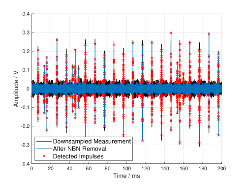
Figure 1: A sample fragment of the noise measurement with preprocessing results.

Then, based on the estimated model parameters, we numerically generate BG and S$\alpha$S noise sequences, each with a length of $5\times 10^{5}$ samples. Subsequently, we compare the empirical PDFs of measured and simulated noise amplitudes. To evaluate the fitnesses of both models, we further calculate the weighted root mean square error (RMSE) for each of them:

$$\epsilon_{\text{model}}=\sqrt{\int_{-\infty}^{+\infty}f_{\text{meas}}(x)[f_{\text{model}}(x)-f_{\text{meas}}(x)]^{2}\text{d}x},$$ (8)

where $f_{\text{meas}}$ and $f_{\text{model}}$ are the empirical PDFs of measured and simulated noise amplitudes, respectively. The results, which are detailed in Section 6.1, demonstrate that both models exhibit fitting performance to a similar degree of satisfaction.

4 Stability of Bernoulli-Gaussian Processes

Towards a unification between the BG and S$\alpha$S models, the first question is: are BG processes stable? To answer this, we test if the BG model defined in (3) fulfills the requirement of stability defined in (5). Consider two idenpendent and identically distributed (i.i.d.) variables $X$ and $Y$ which are generated according to (3), and their sum $W$:

$$w(k)=x(k)+y(k),\forall k\in\mathbb{Z}.$$ (9)

The PDF of $W$ will then be

$$f_{W}(w)=\int\limits_{-\infty}^{+\infty}f_{Y}(w-x)f_{X}(x)\mathrm{d}x.$$ (10)

As both $X$ and $Y$ have the same PDF as given in (4), we have

$$\begin{split}&f_{W}(w)=\int\limits_{-\infty}^{+\infty}f_{\textrm{BG}}(w-x)f_{\textrm{BG}}(x)\mathrm{d}x\\ =&\frac{1-2p+p^{2}}{\sqrt{4\pi\sigma_{\textrm{B}}^{2}}}\mathrm{e}^{-\frac{w^{2}}{4\sigma_{\textrm{B}}^{2}}}+\frac{p^{2}}{\sqrt{4\pi(\sigma_{\textrm{B}}^{2}+\sigma_{\textrm{I}}^{2})}}\mathrm{e}^{-\frac{w^{2}}{4(\sigma_{\textrm{B}}^{2}+\sigma_{\textrm{I}}^{2})}}\\ +&\frac{p-p^{2}}{\sqrt{2\pi(2\sigma_{\textrm{B}}^{2}+\sigma_{\textrm{I}}^{2})}}\left(\mathrm{e}^{-\frac{(2\sigma_{\textrm{B}}^{2}+\sigma_{\textrm{I}}^{2}-1)w^{2}}{2(\sigma_{\textrm{B}}^{2}+\sigma_{\textrm{I}}^{2})(2\sigma_{\textrm{B}}^{2}+\sigma_{\textrm{I}}^{2})}}+\mathrm{e}^{-\frac{(2\sigma_{\textrm{B}}^{2}+\sigma_{\textrm{I}}^{2}-1)w^{2}}{2\sigma_{\textrm{B}}^{2}(2\sigma_{\textrm{B}}^{2}+\sigma_{\textrm{I}}^{2})}}\right).\end{split}$$ (11)

Clearly, (11) differs in form from (4), so that we know Bernoulli-Gaussian processes are not generally stable. Only in the following three special cases, $W$ is quasi-stable as it approximately approaches to a Gaussian process:

$$\lim\limits_{p\to 0}f_{W}\left(\frac{w}{\sqrt{2}}\right) =\lim\limits_{p\to 0}f_{\textrm{BG}}(w)\approx f_{\textrm{B}}(w);$$ (12)

$$\lim\limits_{p\to 1}f_{W}\left(\frac{w}{\sqrt{2}}\right) =\lim\limits_{p\to 1}f_{\textrm{BG}}(w)\approx f_{\textrm{I}}(w);$$ (13)

$$\lim\limits_{\sigma_{\textrm{I}}^{2}-\sigma_{\textrm{B}}^{2}\to 0}f_{W}\left(\frac{w}{\sqrt{2}}\right) =f_{\textrm{BG}}(w)\approx f_{\textrm{B}}(w)\approx f_{\textrm{I}}(w),$$ (14)

where $f_{\textrm{B}}(w)$ and $f_{\textrm{I}}(w)$ are the PDFs of $n_{\textrm{B}}(k)$ and $n_{\textrm{I}}(k)$, respectively. The approximation (12) is valid in the context of PLC, where $p$ is sufficiently low although $\sigma_{\textrm{I}}^{2}$ is significantly higher than $\sigma_{\textrm{B}}^{2}$, as it will be demonstrated and discussed with details in Section 6.2.

5 Estimating S$\alpha$S Parameters of BG Processes

So far, we have demonstrated a certain but limited compatibility between the BG and S$\alpha$S models for power line noises. Subsequently, driven by the interest in the performance of approximating BG models with S$\alpha$S models, we attempt to apply the S$\alpha$S model on BG processes.

Our methodology can be summarized as follows. First, we generate a BG noise with parameters $(p,\sigma_{\textrm{B}}=1,\sigma_{\textrm{I}})$, and normalize it to $n_{\textrm{BG}}$ with unity power. Then we apply McColloch’s S$\alpha$S parameter estimator [18] on it. Subsequently, we call Chambers’ method [19] to simulate a S$\alpha$S noise sequence $n_{\textrm{S$\alpha$S}}$ with the estimated parameters $(\hat{\alpha},\hat{\gamma})$. Afterwards, we evaluate the fitting performance with the Kullback-Leibler divergence  [20]:

$$D_{\textrm{KL}}(\phi_{\textrm{BG}}|\phi_{\textrm{S$\alpha$S}})=\int\limits_{-\infty}^{+\infty}\phi_{\textrm{BG}}(x)\ln\frac{\phi_{\textrm{BG}}(x)}{\phi_{\textrm{S$\alpha$S}}(x)}\mathrm{d}x,$$ (15)

where $\phi_{\textrm{BG}}$ and $\phi_{\textrm{S$\alpha$S}}$ denote the empirical PDF of $n_{\textrm{BG}}$ and $n_{\textrm{S$\alpha$S}}$, respectively. This divergence, also known as the relative entropy, is normalized to the range $[0,1]$ and measures the degree that $\phi_{\textrm{BG}}$ diverges from $\phi_{\textrm{S$\alpha$S}}$. $D_{\textrm{KL}}(\phi_{\textrm{BG}}|\phi_{\textrm{S$\alpha$S}})=0$ indicates that both the distributions are highly similar, if not the same, while $D_{\textrm{KL}}(\phi_{\textrm{BG}}|\phi_{\textrm{S$\alpha$S}})=1$ denotes a minimal similarity between the distributions. By repeating this process with different Bernoulli-Gaussian parameters, we are able to investigate the dependencies of $(\hat{\alpha},\hat{\gamma})$ on $(p,{\sigma_{\textrm{I}}^{2}}/{\sigma_{\textrm{B}}^{2}})$.

Due to the lack of closed-form density functions, most conventional analytic methods of statistics cannot be applied to estimate S$\alpha$S parameters for cases where $\alpha>1$. Nevertheless, a variety of numerical techniques have been developed for this task. According to  [14], classical approaches can be generally classified into four categories: methods of maximum likelihood [21, 22], methods of sample fractiles [18, 8], methods of sample characteristic functions [23, 24]. Besides, some recent methods have been developed based on other principles e.g. negative-order moments  [25], extreme order statistics [8] and point process [26].

As we have derived in Section 4, BG processes are not strictly stable. This disqualifies the deployment of some methods listed above on data generated by the BG model, especially the methods that require segmentation of the sample data. For instance, according to our experiment, the extreme-order-statistics-based estimators in [8] significantly depend on the sample size, and fail to converge, as shown in Fig. 2.

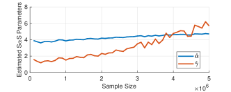
Figure 2: Tsihrintzis’s extreme-order-statistic-based estimators in [8] of S$\alpha$S model fail to converge when applied on Bernoulli-Gaussian distributed data. The segmentation parameter of the approach is set to $\left\lfloor\sqrt{N}\right\rfloor$, where $N$ is the sample size.

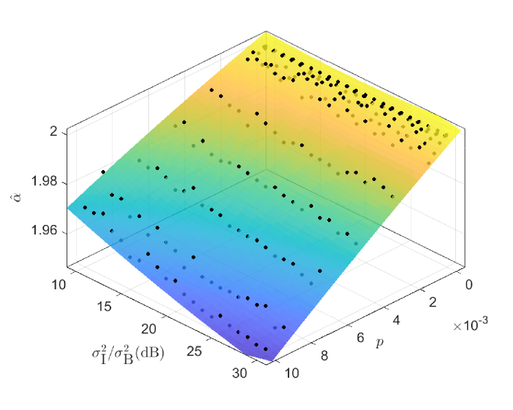
(a) Estimated S$\alpha$S parameter $\hat{\alpha}$, with the polynomially fitted surface

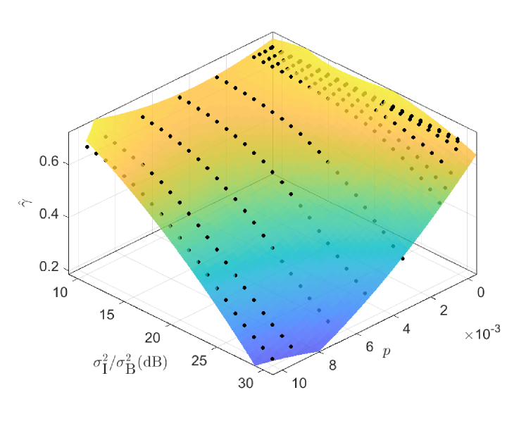
(b) Estimated S$\alpha$S parameter $\hat{\gamma}$, with the polynomially fitted surface

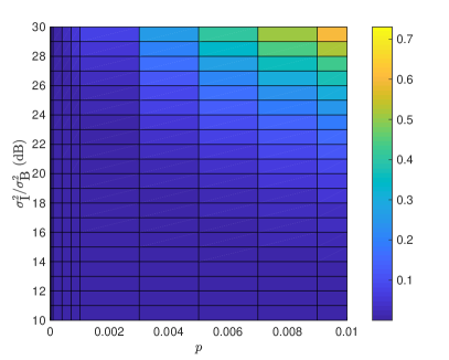
(c) The Kullback-Leibler divergence $D_{\textrm{KL}}(\phi_{\textrm{BG}}|\phi_{\textrm{S$\alpha$S}})$

Figure 3: Applying the S$\alpha$S model on Bernoulli-Gaussian noises with different specifications. Under each specification, $5\times 10^{6}$ samples of noise are generated.

Nevertheless, our experiments have proved that at least the regressive methods of Koutrouvelis  [27, 23] and McCulloch  [18] can be applied, which return similar results. We provide sample outputs obtained by McCulloch’s estimators in Section 6.3.

6 Results and Discussion

6.1 Fitness Test of Models on Field Measurements

The fitting results of BG and S$\alpha$S models on field measurements mentioned in Section 3 are illustrated in Fig. 4, with the RMSEs listed in Tab. 1. It can be summarized that:

1. Both BG and S$\alpha$S models are able to effectively describe the amplitude distribution of PLC noises, although not perfectly.

2. When applied on the same PLC noise, the S$\alpha$S model gives a wider main lobe in PDF than the measurement, while the BG model has a narrower main lobe than the measurement.

3. For both models, the fitting performance varies with the noise scenario.

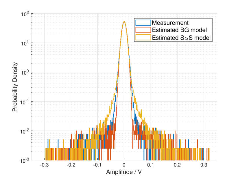
(a) Noise measured on September 9^th at 18:17

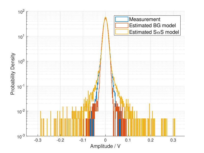
(b) Noise measured on September 14^th at 01:08

Figure 4: Fitting the noise statistics with BG and S$\alpha$S models.

Table 1: Weighted RMSEs of the BG and S$\alpha$S models on PLC noise measurements.

	Sept. 9, 18:17	Sept. 14, 01:08
BG	0.0044	0.0019
S$\alpha$S	0.0039	0.0134

6.2 Stability Test of BG Distribution

To verify (12)–(14), we conducted numerical simulations: three i.i.d. BG random variables $X,Y,Z$ were generated, and another variable $V$ was obtained by $V=(X+Y)\times\sqrt{\frac{\textrm{Var}(Z)}{\textrm{Var}(X+Y)}}$. Then we compared the PDFs of $V$ and $Z$ under different BG model specifications.

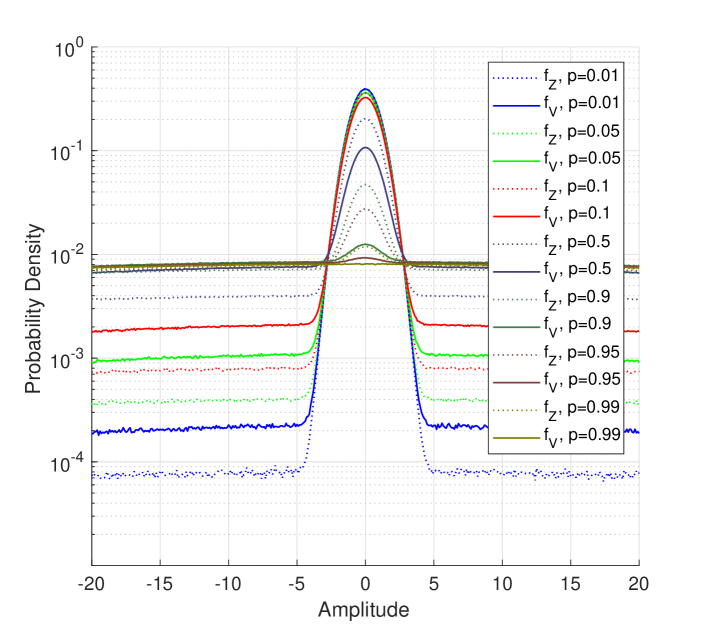
(a) BG distribution with different impulse ratios. $\sigma_{\textrm{B}}=1$, $\sigma_{\textrm{I}}=50$.

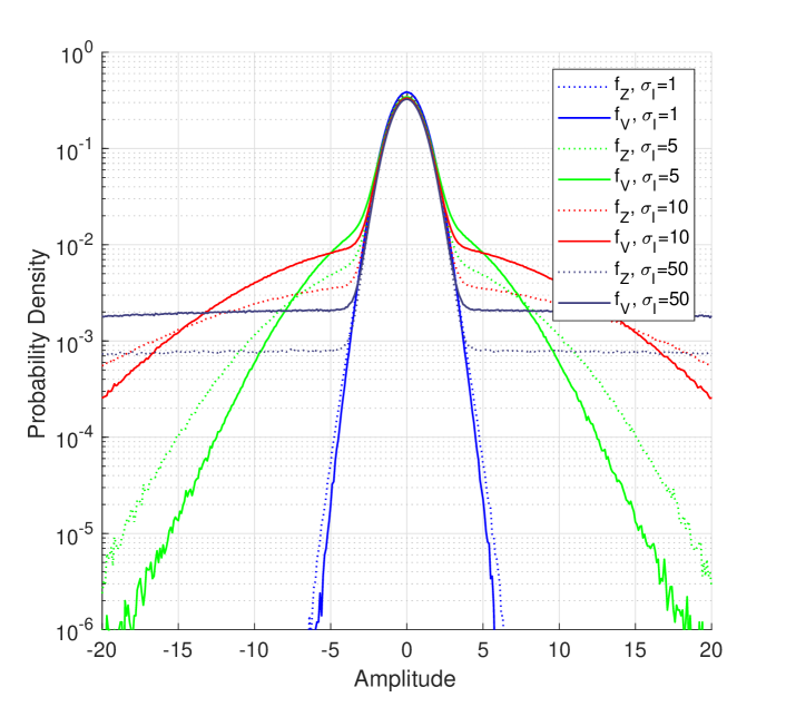
(b) BG distribution with different impulse deviations. $p=0.1$, $\sigma_{\textrm{B}}=1$.

Figure 5: Testing the stability of BG distribution with respect to the model parameters.

First, the deviations were fixed to $\sigma_{\textrm{B}}=1$ and $\sigma_{\textrm{I}}=50$, and the test was executed for different values of $p$. The results are shown in Fig. 5(a). It can be observed that the PDFs of $V$ and $Z$ match each other well when the value of $p$ is sufficiently high or low, but deviate from each other as $p$ approaches to $0.5$, which matches our theory. Subsequently, we set $p=0.1$, $\sigma_{\textrm{B}}^{2}=1$, and repeated the test for different values of $\sigma_{\textrm{I}}$. The results in Fig. 5(b) show that $V$ has its distribution more similar to $Z$ under lower impulse power, as we have expected.

In the context of PLC, according to  [28], over the broad band up to $20\text{\,}\mathrm{MHz}$, the impulse power is usually by $10\text{\,}\mathrm{dB}30\text{\,}\mathrm{dB}$, i.e., 10 to 1000 times higher than that of the background noise. Meanwhile, the impulse probability remains below $0.35\%$ even under the heaviest disturbance, and falls down to $0.00135\%$ under the weak disturbance. Comparing these to the result in Fig. 5(a), it is reasonable to consider the BG model as quasi-stable when applied on power line noises.

6.3 S$\alpha$S Parameter Estimation of BG Processes

Setting $\sigma_{\textrm{B}}=1$ with different values of $0.01\%\leq p\leq 1\%$ and $$10\text{\,}\mathrm{dB}$\leq\frac{\sigma_{\textrm{I}}^{2}}{\sigma_{\textrm{B}}^{2}}\leq$30\text{\,}\mathrm{dB}$$, we applied McCulloch’s estimators on randomly generated BG processes, and got the results in Fig. 3. We can observe from the Kullback-Leibler divergence that the conversion can successfully provide a precise approximation when either the impulse-to-background power ratio $\frac{\sigma_{\textrm{I}}^{2}}{\sigma_{\textrm{B}}^{2}}$ or the impulse ratio $p$ is limited. In the cases with extremely intensive impulses where both $\frac{\sigma_{\textrm{I}}^{2}}{\sigma_{\textrm{B}}^{2}}$ and $p$ are high, the fitness of model conversion sinks dramatically. We also fitted (2,2)-polynomial surfaces for $\hat{\alpha}$ and $\hat{\gamma}$ to support fast and approximate conversions from power-normalized BG model to S$\alpha$S model, the results are listed in Tab. 2.

Table 2: (2,2)-polynomial surface fitting results of $\hat{\alpha}$ and $\hat{\gamma}$ as function of $p$ and $\frac{\sigma_{\textrm{I}}}{\sigma_{\textrm{B}}}$.

	$\hat{\alpha}$	$\hat{\gamma}$
$c_{00}$	2.005	0.5779
$c_{10}$	-1.457	6.256
$c_{01}$	$-5.575\times 10^{-4}$	0.01707
$c_{20}$	-40.36	2123
$c_{11}$	-0.1128	-2.43
$c_{02}$	$1.426\times 10^{-5}$	$-5.249\times 10^{-4}$
RMSE	$1.715\times 10^{-3}$	$2.433\times 10^{-2}$
Fitting model: $f(x,y)=c_{00}+c_{10}x+c_{01}y+c_{20}x^{2}$
$+c_{11}xy+c_{02}y^{2}$, where $x=p$, $y=20\log_{10}(\sigma_{\textrm{I}}/\sigma_{\textrm{B}})$

7 Conclusion

In this paper, we have studied the compatibility between two widely-used models for impulsive power line noises: the BG model and the S$\alpha$S model. With field measurement test, we have proved that they give different but similarly acceptable results when used to model power line noise. Then we have proved that the BG distribution is neither strictly stable nor strictly fat-tailed, so that no analytical unification between BG and S$\alpha$S models is feasible. Nevertheless, when the impulses are sparse and not extremely strong in power, which is the common case of power line noises, BG processes can be approximately considered as quasi-stable, so that an approximate and empirical model conversion is possible. Based on this result, we have proposed a fast (2,2)-polynomial conversion from BG model to S$\alpha$S model. This fast conversion can be applied to merge reference power line noise scenarios based on different models, and hence to simplify the performance evaluation of PLC systems.

Appendix A The PDF of Sum of Two I.I.D. BG Noises

The detailed derivation of (11) follows below:

$$\begin{split}&f_{W}(w)=\int\limits_{-\infty}^{+\infty}f_{\textrm{BG}}(w-x)f_{\textrm{BG}}(x)\mathrm{d}x\\ =&\int\limits_{-\infty}^{+\infty}\left[\frac{1-p}{\sqrt{2\pi\sigma_{\textrm{B}}^{2}}}\mathrm{e}^{-\frac{(w-x)^{2}}{2\sigma_{\textrm{B}}^{2}}}+\frac{p}{\sqrt{2\pi(\sigma_{\textrm{B}}^{2}+\sigma_{\textrm{I}}^{2})}}\mathrm{e}^{-\frac{(w-x)^{2}}{2(\sigma_{\textrm{B}}^{2}+\sigma_{\textrm{I}}^{2})}}\right]\\ &\times\left[\frac{1-p}{\sqrt{2\pi\sigma_{\textrm{B}}^{2}}}\mathrm{e}^{-\frac{x^{2}}{2\sigma_{\textrm{B}}^{2}}}+\frac{p}{\sqrt{2\pi(\sigma_{\textrm{B}}^{2}+\sigma_{\textrm{I}}^{2})}}\mathrm{e}^{-\frac{x^{2}}{2(\sigma_{\textrm{B}}^{2}+\sigma_{\textrm{I}}^{2})}}\right]\mathrm{d}x\\ =&\int\limits_{-\infty}^{+\infty}\left[\frac{(1-p)^{2}}{2\pi\sigma_{\textrm{B}}^{2}}\mathrm{e}^{-\frac{(w-x)^{2}+x^{2}}{2\sigma_{\textrm{B}}^{2}}}+\frac{p^{2}}{2\pi(\sigma_{\textrm{B}}^{2}+\sigma_{\textrm{I}}^{2})}\mathrm{e}^{-\frac{(w-x)^{2}+x^{2}}{2(\sigma_{\textrm{B}}^{2}+\sigma_{\textrm{I}}^{2})}}\right.\\ &\left.+\frac{p(1-p)}{2\pi\sigma_{\textrm{B}}\sqrt{\sigma_{\textrm{B}}^{2}+\sigma_{\textrm{I}}^{2}}}\left(\mathrm{e}^{-\frac{(w-x)^{2}}{2(\sigma_{\textrm{B}}^{2}+\sigma_{\textrm{I}}^{2})}-\frac{x^{2}}{2\sigma_{\textrm{B}}^{2}}}+\mathrm{e}^{-\frac{x^{2}}{2(\sigma_{\textrm{B}}^{2}+\sigma_{\textrm{I}}^{2})}-\frac{(w-x)^{2}}{2\sigma_{\textrm{B}}^{2}}}\right)\right]\mathrm{d}x\\ =&\int\limits_{-\infty}^{+\infty}\frac{(1-p)^{2}}{2\pi\sigma_{\textrm{B}}^{2}}\mathrm{e}^{-\frac{2x^{2}-2wx+w^{2}}{2\sigma_{\textrm{B}}^{2}}}\mathrm{d}x+\int\limits_{-\infty}^{+\infty}\frac{p^{2}}{2\pi(\sigma_{\textrm{B}}^{2}+\sigma_{\textrm{I}}^{2})}\mathrm{e}^{-\frac{2x^{2}-2wx+w^{2}}{2(\sigma_{\textrm{B}}^{2}+\sigma_{\textrm{I}}^{2})}}\mathrm{d}x\\ +&\int\limits_{-\infty}^{+\infty}\frac{p(1-p)}{2\pi\sigma_{\textrm{B}}\sqrt{\sigma_{\textrm{B}}^{2}+\sigma_{\textrm{I}}^{2}}}\left(\mathrm{e}^{-\frac{(2\sigma_{\textrm{B}}^{2}+\sigma_{\textrm{I}}^{2})x^{2}-2\sigma_{\textrm{B}}^{2}wx+\sigma_{\textrm{B}}^{2}w^{2}}{2\sigma_{\textrm{B}}^{2}(\sigma_{\textrm{B}}^{2}+\sigma_{\textrm{I}}^{2})}}\right.\\ &\left.+\mathrm{e}^{-\frac{(2\sigma_{\textrm{B}}^{2}+\sigma_{\textrm{I}}^{2})x^{2}-2(\sigma_{\textrm{B}}^{2}+\sigma_{\textrm{I}}^{2})wx+(\sigma_{\textrm{B}}^{2}+\sigma_{\textrm{I}}^{2})w^{2}}{2\sigma_{\textrm{B}}^{2}(\sigma_{\textrm{B}}^{2}+\sigma_{\textrm{I}}^{2})}}\right)\mathrm{d}x.\end{split}$$ (16)

Let $\sigma_{1}=\sqrt{\sigma_{\textrm{B}}^{2}+\sigma_{\textrm{I}}^{2}}$, $\sigma_{2}=\sqrt{2\sigma_{\textrm{B}}^{2}+\sigma_{\textrm{I}}^{2}}=\sqrt{\sigma_{\textrm{B}}^{2}+\sigma_{1}^{2}}$:

$$\begin{split}f_{W}(w)=&\frac{(1-p)^{2}}{2\pi\sigma_{\textrm{B}}^{2}}\int\limits_{-\infty}^{+\infty}\mathrm{e}^{-\frac{2x^{2}-2wx+w^{2}}{2\sigma_{\textrm{B}}^{2}}}\mathrm{d}x+\frac{p^{2}}{2\pi\sigma_{1}^{2}}\int\limits_{-\infty}^{+\infty}\mathrm{e}^{-\frac{2x^{2}-2wx+w^{2}}{2\sigma_{1}^{2}}}\mathrm{d}x\\ &+\frac{p(1-p)}{2\pi\sigma_{\textrm{B}}\sigma_{1}}\int\limits_{-\infty}^{+\infty}\left(\mathrm{e}^{-\frac{\sigma_{2}^{2}x^{2}-2\sigma_{\textrm{B}}^{2}wx+\sigma_{\textrm{B}}^{2}w^{2}}{2\sigma_{\textrm{B}}^{2}\sigma_{1}^{2}}}+\mathrm{e}^{-\frac{\sigma_{2}^{2}x^{2}-2\sigma_{1}^{2}wx+\sigma_{1}^{2}w^{2}}{2\sigma_{\textrm{B}}^{2}\sigma_{1}^{2}}}\right)\mathrm{d}x\\ =&\frac{1-2p+p^{2}}{\sqrt{4\pi\sigma_{\textrm{B}}^{2}}}\mathrm{e}^{-\frac{w^{2}}{4\sigma_{\textrm{B}}^{2}}}\int\limits_{-\infty}^{+\infty}\frac{1}{\sqrt{2\pi\sigma_{\textrm{B}}^{2}}}\mathrm{e}^{-\frac{\left(\sqrt{2}x-\frac{\sqrt{2}}{2}w\right)^{2}}{2\sigma_{\textrm{B}}^{2}}}\mathrm{d}\left(\sqrt{2}x-\frac{\sqrt{2}}{2}w\right)\\ &+\frac{p^{2}}{\sqrt{4\pi\sigma_{1}^{2}}}\mathrm{e}^{-\frac{w^{2}}{4\sigma_{1}^{2}}}\int\limits_{-\infty}^{+\infty}\frac{1}{\sqrt{2\pi\sigma_{1}^{2}}}\mathrm{e}^{-\frac{\left(\sqrt{2}x-\frac{\sqrt{2}}{2}w\right)^{2}}{2\sigma_{1}^{2}}}\mathrm{d}\left(\sqrt{2}x-\frac{\sqrt{2}}{2}w\right)\\ +&\frac{p-p^{2}}{\sqrt{2\pi\sigma_{2}^{2}}}\mathrm{e}^{-\frac{(\sigma_{2}^{2}-1)w^{2}}{2\sigma_{1}^{2}\sigma_{2}^{2}}}\int\limits_{-\infty}^{+\infty}\frac{1}{\sqrt{2\pi\sigma_{\textrm{B}}^{2}\sigma_{1}^{2}}}\mathrm{e}^{-\frac{\left(\sigma_{2}x-\frac{\sigma_{\textrm{B}}}{\sigma_{2}}w\right)^{2}}{2\sigma_{\textrm{B}}^{2}\sigma_{1}^{2}}}\textrm{d}\left(\sigma_{2}x-\frac{\sigma_{\textrm{B}}}{\sigma_{2}}w\right)\\ &+\frac{p-p^{2}}{\sqrt{2\pi\sigma_{2}^{2}}}\mathrm{e}^{-\frac{(\sigma_{2}^{2}-1)w^{2}}{2\sigma_{\textrm{B}}^{2}\sigma_{2}^{2}}}\int\limits_{-\infty}^{+\infty}\frac{1}{\sqrt{2\pi\sigma_{\textrm{B}}^{2}\sigma_{1}^{2}}}\mathrm{e}^{-\frac{\left(\sigma_{2}x-\frac{\sigma_{1}}{\sigma_{2}}w\right)^{2}}{2\sigma_{\textrm{B}}^{2}\sigma_{1}^{2}}}\textrm{d}\left(\sigma_{2}x-\frac{\sigma_{1}}{\sigma_{2}}w\right).\end{split}$$ (17)

Note that all the integration terms in the last step of (17) follow the form of normal distribution. Hence, all the integrations over $(-\infty,\infty)$ have the value of 1, and we get:

$$\begin{split}f_{\textrm{W}}(w)=&\frac{1-2p+p^{2}}{\sqrt{4\pi\sigma_{\textrm{B}}^{2}}}\mathrm{e}^{-\frac{w^{2}}{4\sigma_{\textrm{B}}^{2}}}+\frac{p^{2}}{\sqrt{4\pi\sigma_{1}^{2}}}\mathrm{e}^{-\frac{w^{2}}{4\sigma_{1}^{2}}}\\ +&\frac{p-p^{2}}{\sqrt{2\pi\sigma_{2}^{2}}}\left(\mathrm{e}^{-\frac{(\sigma_{2}^{2}-1)w^{2}}{2\sigma_{1}^{2}\sigma_{2}^{2}}}+\mathrm{e}^{-\frac{(\sigma_{2}^{2}-1)w^{2}}{2\sigma_{\textrm{B}}^{2}\sigma_{2}^{2}}}\right).\end{split}$$ (18)

References

- [1] D. Middleton, Procedures for Determining the Parameters of the First-Order Canonical Models of Class A and Class B Electromagnetic Interference, Transactions on Electromagnetic Compatibility (3) (1979) 190–208.
- [2] M. Ghosh, Analysis of the Effect of Impulse Noise on Multicarrier and Single Carrier QAM Systems, IEEE Transactions on Communications 44 (2) (1996) 145–147.
- [3] G. Laguna-Sanchez, M. Lopez-Guerrero, An Experimental Study of the Effect of Human Activity on the Alpha-Stable Characteristics of the Power-Line Noise, in: 18th IEEE International Symposium on Power Line Communications and its Applications (ISPLC), IEEE, 2014, pp. 6–11.
- [4] G. Ndo, F. Labeau, M. Kassouf, A Markov-Middleton Model for Bursty Impulsive Noise: Modeling and Receiver Design, IEEE Transactions on Power Delivery 28 (4) (2013) 2317–2325.
- [5] D. Fertonani, G. Colavolpe, On Reliable Communications over Channels Impaired by Bursty Impulse Noise, IEEE Transactions on Communications 57 (7).
- [6] T. Shongwe, A. J. H. Vinck, H. C. Ferreira, On Impulse Noise and Its Models, in: 18th IEEE International Symposium on Power Line Communications and its Applications (ISPLC), IEEE, 2014, pp. 12–17.
- [7] B. Han, V. Stoica, C. Kaiser, N. Otterbach, K. Dostert, Noise Characterization and Emulation for Low-Voltage Power Line Channels across Narrowband and Broadband, Digital Signal Processing 69 (2017) 259–274.
- [8] G. A. Tsihrintzis, C. L. Nikias, Fast Estimation of the Parameters of Alpha-Stable Impulsive Interference, IEEE Transactions on Signal Processing 44 (6) (1996) 1492–1503.
- [9] W. Liu, G. Bumiller, H. Gao, On (Power-) Line Defined PLC System, in: 2014 18th IEEE International Symposium on Power Line Communications and its Applications (ISPLC), IEEE, 2014, pp. 81–86.
- [10] S. Galli, A. Scaglione, Z. Wang, For the Grid and through the Grid: The Role of Power Line Communications in the Smart Grid, Proceedings of the IEEE 99 (6) (2011) 998–1027.
- [11] J. A. Cortés, L. Diez, F. J. Canete, J. J. Sanchez-Martinez, Analysis of the Indoor Broadband Power-Line Noise Scenario, IEEE Transactions on electromagnetic compatibility 52 (4) (2010) 849–858.
- [12] J. Lin, M. Nassar, B. L. Evans, Non-parametric Impulsive Noise Mitigation in OFDM Systems Using Sparse Bayesian Learning, in: 2011 IEEE Global Telecommunications Conference (GLOBECOM), IEEE, 2011, pp. 1–5.
- [13] J. P. Nolan, Stable Distributions - Models for Heavy Tailed Data, Birkhauser, Boston, 2017, in progress, Chapter 1 online at http://fs2.american.edu/jpnolan/www/stable/stable.html.
- [14] C. L. Nikias, M. Shao, Signal Processing with Alpha-Stable Distributions and Applications, Wiley-Interscience, New York, NY, USA, 1995.
- [15] G. Laguna-Sanchez, M. Lopez-Guerrero, On the Use of Alpha-Stable Distributions in Noise Modeling for PLC, IEEE Transactions on Power Delivery 30 (4) (2015) 1863–1870.
- [16] B. Han, H. D. Schotten, A Fast Blind Impulse Detector for Bernoulli-Gaussian Noise in Underspread Channel, in: 2018 IEEE International Conference on Communications (ICC), IEEE, 2018, pp. 1–6.
- [17] B. Han, C. Kaiser, K. Dostert, A Novel Approach of Canceling Cyclostationary Noises in Low-Voltage Powerline Communications, in: International Conference on Communications (ICC), IEEE, 2015.
- [18] J. H. McCulloch, Simple Consistent Estimators of Stable Distribution Parameters, Communications in Statistics-Simulation and Computation 15 (4) (1986) 1109–1136.
- [19] J. M. Chambers, C. L. Mallows, B. Stuck, A Method for Simulating Stable Random Variables, Journal of the American Statistical Association 71 (354) (1976) 340–344.
- [20] S. Kullback, Information Theory and Statistics, Courier Corporation, 1997.
- [21] B. W. Brorsen, S. R. Yang, Maximum Likelihood Estimates of Symmetric Stable Distribution Parameters, Communications in Statistics-Simulation and Computation 19 (4) (1990) 1459–1464.
- [22] J. P. Nolan, Maximum Likelihood Estimation and Diagnostics for Stable Distributions, Lévy Processes: Theory and Applications (2001) 379–400.
- [23] I. A. Koutrouvelis, An Iterative Procedure for the Estimation of the Parameters of Stable Laws: An Iterative Procedure for the Estimation, Communications in Statistics-Simulation and Computation 10 (1) (1981) 17–28.
- [24] S. M. Kogon, D. B. Williams, Characteristic Function Based Estimation of Stable Distribution Parameters, A Practical Guide to Heavy Tailed Data (1998) 311–335.
- [25] X. Ma, C. L. Nikias, On Blind Channel Identification for Impulsive Signal Environments, in: 1995 International Conference on Acoustics, Speech, and Signal Processing (ICASSP), Vol. 3, IEEE, 1995, pp. 1992–1995.
- [26] F. Marohn, Estimating the Index of a Stable Law via the Pot-Method, Statistics & Probability Letters 41 (4) (1999) 413–423.
- [27] I. A. Koutrouvelis, Regression-Type Estimation of the Parameters of Stable Laws, Journal of the American Statistical Association 75 (372) (1980) 918–928.
- [28] M. Zimmermann, K. Dostert, An Analysis of the Broadband Noise Scenario in Powerline Networks, in: International Symposium on Powerline Communications and its Applications (ISPLC), IEEE, 2000, pp. 5–7.