Tameness of Margulis space-times with parabolics

Abstract.

Let $\mathsf{E}$ be a flat Lorentzian space of signature $(2,1)$. A Margulis space-time is a noncompact complete Lorentz flat $3$-manifold $\mathsf{E}/\Gamma$ with a free holonomy group $\Gamma$ of rank $\mathsf{g},\mathsf{g}\geq 2$. We consider the case when $\Gamma$ contains a parabolic element. We obtain a characterization of proper $\Gamma$-actions in terms of Margulis and Drumm-Charette invariants. We show that $\mathsf{E}/\Gamma$ is homeomorphic to the interior of a compact handlebody of genus $\mathsf{g}$ generalizing our earlier result. Also, we obtain a bordification of the Margulis space-time with parabolics by adding a real projective surface at infinity giving us a compactification as a manifold relative to parabolic end neighborhoods. Our method is to estimate the translational parts of the affine transformation group and use some $3$-manifold topology.

1. Introduction

Let ${\mathbf{Isom}}^{+}(\mathsf{E})$ denote the group of orientation-preserving Lorentzian isometries on the oriented flat Lorentzian space $\mathsf{E}$ of the signature $(2,1)$. Here, we have an exact sequence

$$1\rightarrow{\mathbb{R}}^{2,1}\rightarrow{\mathbf{Isom}}^{+}(\mathsf{E})\stackrel{{\scriptstyle\mathcal{L}}}{{\longrightarrow}}{\mathsf{SO}}(2,1)\rightarrow 1$$

where $\mathcal{L}$ is the homomorphism taking the linear parts of the isometries. A parabolic of ${\mathbf{Isom}}^{+}(\mathsf{E})$ is an element whose linear part is a parabolic element of ${\mathsf{SO}}(2,1)$.

A discrete affine group $\Gamma$ acting properly on $\mathsf{E}$ is either solvable or is free of rank $\geq 2$. (See Goldman-Labourie [28].) While we will assume that $\Gamma$ is a free group of rank $\geq 2$, we say that $\Gamma$ is a proper affine free group of rank $\geq 2$.

We will often require $\mathcal{L}(\Gamma)\subset{\mathsf{SO}}(2,1)^{o}$ for the subgroup ${\mathsf{SO}}(2,1)^{o}$ of ${\mathsf{SO}}(2,1)$ acting on the positive cone. Here, $\mathcal{L}(\Gamma)$ acts properly discontinuously and freely on a hyperbolic plane ${\mathbb{H}}^{2}$ formed by positive rays in the cone. We say that $\Gamma$ is a proper affine hyperbolic group of rank $\mathsf{g}$ with linear parts in ${\mathsf{SO}}(2,1)^{o}$

• if it acts properly discontinuously faithfully and freely on $\mathsf{E}$, and

• $\mathcal{L}(\Gamma)$ is a free group of rank $\mathsf{g},\mathsf{g}\geq 2$ in ${\mathsf{SO}}(2,1)^{o}$, acting freely and discretely on ${\mathbb{H}}^{2}$.

It will be sufficient to prove tameness in this case.

A real projective structure on a manifold is given by a maximal atlas of charts to ${\mathbb{R}}P^{n},n\geq 1,$ with transition maps in ${\mathsf{PGL}}(n+1,{\mathbb{R}})$. A real projective manifold is a manifold with a real projective structure.

Theorem 1.1.

Suppose that $\Gamma$ is a proper affine free group of rank $\mathsf{g},\mathsf{g}\geq 2$, with parabolics and linear parts in ${\mathsf{SO}}(2,1)^{o}$. Then

• $\mathsf{E}/\Gamma$ is diffeomorphic to the interior of a compact handlebody of genus $\mathsf{g}$.

• Moreover, it is the interior of a real projective $3$-manifold $M$ with boundary equal to a totally geodesic real projective surface, and $M$ deformation retracts to a compact handlebody obtained by removing a union of finitely many end-neighborhoods homeomorphic to solid tori.

These real projective surfaces are from the paper of Goldman [27]. The second item is the so-called relative compactification.

For all cases of Margulis space-times, we have

Corollary 1.2.

Let $\Gamma$ be a proper affine free group of rank $\geq 2$ with parabolics. Then $\mathsf{E}/\Gamma$ is diffeomorphic to the interior of a compact handlebody of genus $\mathsf{g}$. Moreover, it is the interior of a real projective $3$-manifold $M$ with boundary equal to a totally geodesic real projective surface, and $M$ deformation-retracts to a compact handlebody obtained by removing a union of finitely many end neighborhoods homeomorphic to solid tori.

We denote by ${\mathbb{S}}$ the sphere of directions in $\mathsf{E}$, by ${\mathbb{S}}_{+}$ the space of directions of positive time-like directions and by ${\mathbb{S}}_{-}$ the space of directions of negative time-like directions. We will consider ${\mathbb{S}}_{+}$ as the projectivization of ${\mathbb{S}}_{+}\cup{\mathbb{S}}_{-}$. Then the quotient space of ${\mathbb{S}}_{+}$ under $\Gamma$ is a complete hyperbolic surface ${\mathsf{S}}$. Let $\mathcal{P}_{\pi_{1}({\mathsf{S}})}$ denote the set of parabolic elements and the identity element of $\pi_{1}({\mathsf{S}})$. We denote by $l_{{\mathbb{S}}_{+}}(g)$ the length of the shortest closed geodesic in ${\mathbb{S}}_{+}/\Gamma$ corresponding to the element $g\in\Gamma$. By Theorem 4.1 of Charette-Drumm [6] generalizing the Margulis opposite sign lemma [40], we will need the following criterion in this paper for our group $\Gamma$.

Criterion 1.1.

Let $\Gamma$ be an isometry group acting on $\mathsf{E}$, and let $\alpha(g)\in{\mathbb{R}}$ for $g\in\Gamma$ denote the Margulis invariant of $g$. $\Gamma$ satisfies the following conditions:

• $\alpha(\gamma)>0$ for every $\gamma\in\pi_{1}({\mathsf{S}})\setminus\mathcal{P}_{\pi_{1}({\mathsf{S}})}$,

• every $\gamma$, $\gamma\in\mathcal{P}_{\pi_{1}({\mathsf{S}})}\setminus\{{\rm I}\}$, has the positive Charette-Drumm invariant, and

• $\alpha(g)\geq c_{{\mathsf{S}}\setminus E}l_{{\mathbb{S}}_{+}}(g)$ for every $g$ realized as a closed geodesic in ${\mathsf{S}}\setminus E$ for the union $E$ of mutually disjoint cusp neighborhoods for a positive constant $c_{{\mathsf{S}}\setminus E}$ depending on ${\mathsf{S}}\setminus E$.

Of course, we can assume the negativity also since the change of the orientation of $\mathsf{E}$ changes the signs of Margulis invariants and Charette Drumm invariants by [22] and [6].

Proposition 1.3.

Suppose that $\Gamma$ acts properly on $\mathsf{E}$. Then Criterion 1.1 holds up to changing the orientation of $\mathsf{E}$.

Proof.

This is proved by Theorem 4.1 of [6] and Lemma 1.4. ∎

Let $\mathsf{U}S$ denote the inverse image of the projection $\mathsf{U}\Sigma\rightarrow\Sigma$ for the the subset $S\subset\Sigma$ and the unit tangent bundle $\mathsf{U}\Sigma$ of a hyperbolic surface $\Sigma$. Let $\mathsf{U}\mathsf{E}$ denote the bundle of unit space-like vectors over $\mathsf{E}$.

Lemma 1.4.

Suppose that $\Gamma$ acts properly on $\mathsf{E}$. Let $E^{\prime}$ be the union of cusp neighborhoods in an $\epsilon$-thin part of ${\mathsf{S}}$. Then there exists a constant $c^{(1.4)}_{{\mathsf{S}}\setminus E^{\prime}}$ in $(0,1)$ depending on $E^{\prime}$ such that for any closed curve $g$ realized as a closed geodesic in ${\mathsf{S}}\setminus E^{\prime}$

$$c^{(1.4)}_{{\mathsf{S}}\setminus E^{\prime}}l_{{\mathbb{S}}_{+}}(g)\leq\alpha(g)\leq\frac{1}{c^{(1.4)}_{{\mathsf{S}}\setminus E^{\prime}}}l_{{\mathbb{S}}_{+}}(g).$$

Proof.

Consider the geodesic currents supported in a compact set $\mathsf{U}{\mathsf{S}}\setminus\mathsf{U}E^{\prime}$. Then the argument of Goldman-Labourie [28] applies to this collection. We have a conjugacy homeomorphism from the set of geodesic currents on $\mathsf{U}{\mathsf{S}}\setminus\mathsf{U}E^{\prime}$ with a compact set of neutral geodesic currents on ${\mathsf{U}}\mathsf{E}/\Gamma$. The length of each of these currents gives us the Margulis invariant. ∎

We prove the following characterization of a proper action of $\Gamma$ in terms of Margulis and Charette-Drumm invariants.

Theorem 1.5.

An affine finitely generated free group $\Gamma$ of rank $\geq 2$ acts properly discontinuously on $\mathsf{E}$ if and only if Criterion 1.1 holds up to a change of the orientation of $\mathsf{E}$.

The forward part is Proposition 1.3. The converse follows from the main result Theorem 4.8 of Section 4. The proof is given at the end of Section 4.6

We mention that the tameness of geometrically finite hyperbolic manifolds was first shown by Marden [36] and later by Thurston [47]. (See Epstein-Marden [23].) Let ${\mathbb{H}}^{3}$ denote the hyperbolic $3$-space. We take the convex hull $\mathcal{CH}(\Lambda)$ in ${\mathbb{H}}^{3}$ of the limit set $\Lambda$ of the Kleinian group $\Gamma$, and there is a deformation retraction of ${\mathbb{H}}^{3}/\Gamma$ to the compact or finite volume $\mathcal{CH}(\Lambda)/\Gamma$ having a thick and thin decomposition. The paper here follows some of Marden’s ideas. (See also Beardon-Maskit [3].)

Also, the approaches here are using thick and thin decomposition ideas of hyperbolic manifolds as suggested by Canary. However, we cannot find a canonical type of decomposition yet and artificially construct the parabolic regions. Only canonically defined regions in analogy to Margulis thin parts in the hyperbolic manifold theory is the regions bounded by parabolic cylinders. (See Section 3.1.2).

Note that the tameness of Margulis space-times without parabolics was shown by Choi and Goldman [16] and Danciger, Guéritaud, and Kassel [19]. Danciger, Guéritaud, and Kassel have also announced a proof [17] for the tameness of Margulis space-times with parabolics, extending [20]. In addition, they give a proof [17] of the crooked plane conjecture in this setting, extending their proof in the setting without parabolics from [20]. Their methods, based on the deformation theory of hyperbolic surfaces, seem very different than those of the present paper.

Differently from them, we directly obtain $3$-dimensional compactification relative to parabolic regions. We estimate by integrals the asymptotics of translation vectors of the affine holonomies. This is done by using the differential form version of the cocycles and estimating with geodesic flows on the vector bundles over the unit tangent bundle of the hyperbolic surface, the uniform Anosov nature of the flow (4.3), and the estimation of the cusp contributions in Appendix B. (See also Goldman-Labourie [28].) In the cusp neighborhoods, we replace the $1$-form with the standard cusp $1$-form and use this to estimate the growth of the cocycles. We use the exponential decreasing of a component of the differential form along the geodesic flows. Then we use estimates of the integration of the standard cusp $1$-forms in Section 4.5.

Using this and the $3$-manifold theory, we show that properly embedded disks and parabolic regions in $\mathsf{E}$ meet the inverse images of compact submanifolds in the Margulis space-time in compact subsets and find fundamental domains.

Since there are many proper affine actions of discrete groups not based on Lie algebraic situations as in [19], [20], [18], and [17], we hope that our method can generalize to these spaces with parabolics providing many points of view. (See Smilga [44], [46], and [45] for example.)

The paper has three parts: the first two sections 2 and 3 are preliminary. Appendices A and B are only dependent on these two sections. Then the main argument parts follow: Section 4 discusses the geometry of the proper affine action, and Section 5 discusses the topology of the quotient space.

In Section 2, we review some projective geometry of Margulis space-times, the hyperbolic geometry of surfaces, Hausdorff convergences, and the Poincaré polyhedron theorem.

In Section 3, we first review the proper action of parabolic elements on the Lorentz space ${\mathbb{R}}^{2,1}$. We analyze the corresponding Lie algebra and vector fields. We introduce a canonical parabolic coordinate system of ${\mathbb{R}}^{2,1}$. In Section 3.2, we generalize the theory of Margulis invariants by Goldman, Labourie, and Margulis [29] and Ghosh and Treib [25] to groups with parabolics. That is, we introduce Charette-Drumm invariants which generalize the Margulis invariants for parabolic elements. In Section 3.3, we will study the parabolic regions and their ruled boundary components.

In Section 4, we will study the limit sets. We show that any sequence of the translation vectors of elements of $\Gamma$, i.e., cocycle elements, will accumulate in terms of directions only to ${\mathbb{S}}_{0}:={\mathbb{S}}\setminus{\mathbb{S}}_{+}\setminus{\mathbb{S}}_{-}$. In key result Corollary 4.9, we will prove that the limit points of a sequence of images of a compact set in ${\mathbb{R}}^{2,1}$ under elements of $\Gamma$ are in ${\mathbb{S}}_{0}$. We will also prove the converse part of the equivalence of the properness of the action and Criterion 1.1, i.e., Theorem 1.5.

In Section 5, we will find the fundamental domain for $M$ bounded by a finite union of properly embedded smooth surfaces showing that $M$ is tame. We prove our main results Theorem 1.1 and Corollary 1.2 here. We make use of parabolic regions bounded by parabolic ruled surfaces. We avoid using almost crooked planes as in [16]. Instead, we are using disks that are partially ruled in parabolic regions to understand the intersections with parabolic regions. We will outline this major section in the beginning.

In Appendix A, we will prove facts about the parabolic regions.

In Appendix B, we will show how to modify $1$-forms representing homology classes. We give estimates of some needed integrals here.

Acknowledgements

We thank Virginie Charette, Jeffrey Danciger, Michael Kapovich, and Fanny Kassel for helpful comments. We thank Richard Canary for the idea to pursue the proof here similar to ones of Marden [36] and Thurston [47] in the Kleinian group theory where they separate the parabolic regions. We thank the MSRI for the hospitality where this work was partially carried out during the program “Dynamics on Moduli Spaces of Geometric Structures” in 2015. Also, we initiated the work during the conference “Exotic Geometric Structures” at the ICERM, Brown University, on September 16-20, 2013.

We do apologize for the length of the article. We felt that the shortening might confuse the readers since we use many ideas in a novel way. Also, dividing the paper seemed a bit unethical and to be a disservice to the mathematical community.

During the preparation of this manuscript, our coauthor Todd Drumm tragically passed away. Todd pioneered the field by developing the geometric approach to Margulis’s breakthough discovery [39] and [40] of proper affine actions of nonabelian free groups. We miss him dearly and dedicate this work to his lasting memory.

2. Preliminary

We will state some necessary facts here, mostly from the paper [16]. Let $\mathsf{E}$ denote the oriented flat Lorentzian space-time given as an affine space with a bilinear inner-product given by

$${\mathsf{B}}(\mathbf{x},\mathbf{x}):=x_{1}^{2}+x_{2}^{2}-x_{3}^{2},\,\mathbf{x}=(x_{1},x_{2},x_{3}).$$

A Lorentzian norm $\left|\mkern-2.0mu\left|\mathbf{x}\right|\mkern-2.0mu\right|$ is given as ${\mathsf{B}}(\mathbf{x},\mathbf{x})^{\frac{1}{2}}$ where $(-1)^{\frac{1}{2}}=i$. We will fix a standard orientation on $\mathsf{E}$ and the associated vector space in this paper. Hence, $\mathsf{E}$ denote an oriented Lorentz space-time.

A Margulis space-time is a manifold of the form $\mathsf{E}/\Gamma$ where $\Gamma$ is a proper affine free subgroup of ${\mathbf{Isom}}(\mathsf{E})$ of rank $\mathbf{g},\mathbf{g}\geq 2$. Elements of ${\mathsf{PSO}}(2,1)$ are hyperbolic, parabolic, or elliptic. An element of ${\mathbf{Isom}}(\mathsf{E})$ is said to be hyperbolic, parabolic, or elliptic if its linear part is so.

The topological boundary ${\rm bd}_{X}A$ of a subset $A$ in another topological space $X$ is given as ${\rm Cl}(A)$ with the set of interior points of $A$ removed. We denote by manifold boundary $\partial A$ and the interior $A^{o}$ of a manifold $A$ as usual. We define the manifold boundary $\partial A:={\rm Cl}(A)\setminus A^{o}$ for any $i$-dimensional manifold $A$ with $i$-dimensional manifold closure ${\rm Cl}(A)$, $i=1,2,3$, in a topological space $X$.

2.1. The projective geometry of the Margulis space-time

Let $V$ be a vector space. Define $\mathbb{P}(V)$ as $V\setminus\{0\}/\sim$ where $\mathbf{x}\sim\mathbf{y}$ iff $\mathbf{x}=s\mathbf{y}$ for $s\in{\mathbb{R}}\setminus\{0\}$. Denote by ${\mathsf{PGL}}(V)$ the group of automorphisms induced by ${\mathsf{GL}}(V)$ on $\mathbb{P}(V)$.

Define the projective sphere ${\mathbb{S}}(V):=V\setminus\{0\}/\sim_{+}\hbox{ where }\mathbf{x}\sim_{+}\mathbf{y}\hbox{ iff }\mathbf{x}=s\mathbf{y}\hbox{ for }s\in{\mathbb{R}}_{+}$. There is a double cover ${\mathbb{S}}(V)\rightarrow\mathbb{P}(V)$ with the deck transformation group generated by the antipodal map $\mathcal{A}:{\mathbb{S}}(V)\rightarrow{\mathbb{S}}(V)$. We will denote by $\left(\mkern-4.0mu\left(\mathbf{v}\right)\mkern-4.0mu\right)$ the equivalence class of $\mathbf{v}$. Let $a_{-}=\mathcal{A}(a)$ denote the antipodal point of $a$. Also, given a set $A\subset{\mathbb{S}}(V)$, we define $A_{-}=\mathcal{A}(A)$. Let ${\mathsf{SL}}_{\pm}(V)$ denote the group of linear maps of determinant $\pm 1$. ${\mathsf{SL}}_{\pm}(V)$ acts on ${\mathbb{S}}(V)$ effectively and transitively.

We embed $\mathsf{E}$ as an open hemisphere in ${\mathbb{S}}({\mathbb{R}}^{4})$ by sending

$$(x_{1},x_{2},x_{3})\hbox{ to }\,\left(\mkern-4.0mu\left(1,x_{1},x_{2},x_{3}\right)\mkern-4.0mu\right)\,\hbox{ for }x_{1},x_{2},x_{3}\in{\mathbb{R}}.$$

The boundary of $\mathsf{E}$ is a great sphere ${\mathbb{S}}$ given by $x_{0}=0$. The rays of the positive cone end in an open disk ${\mathbb{S}}_{+}\subset{\mathbb{S}}$, and the rays of the negative cone end in an open disk ${\mathbb{S}}_{-}\subset{\mathbb{S}}$ where $\mathcal{A}({\mathbb{S}}_{\pm})={\mathbb{S}}_{\mp}$. The closure of $\mathsf{E}$ is a $3$-hemisphere $\mathcal{H}$ bounded by ${\mathbb{S}}$.

The group ${\mathbf{Isom}}^{+}(\mathsf{E})$ of orientation-preserving isometries acts on $\mathsf{E}$ as a group of affine transformations and hence extends to a group ${\mathsf{SL}}_{\pm}({\mathbb{R}}^{4})$ of projective automorphisms of ${\mathbb{S}}({\mathbb{R}}^{4})$. It restricts to the projective automorphism groups of $\mathcal{H}$ and of ${\mathbb{S}}$ and ${\mathbb{S}}_{\pm}$ respectively.

2.2. Thin parts of hyperbolic surfaces

As a subgroup of ${\mathsf{SL}}_{\pm}({\mathbb{R}}^{3})\subset{\mathsf{SL}}_{\pm}({\mathbb{R}}^{4})$, the Lorentz group ${\mathsf{SO}}(2,1)$ acts on ${\mathbb{S}}_{+}\cup{\mathbb{S}}_{-}$ where ${\mathsf{SO}}(2,1)^{o}$ is the subgroup acting on ${\mathbb{S}}_{+}$ and is an index two subgroup. The space ${\mathbb{S}}_{+}\cup{\mathbb{S}}_{-}$ carries a ${\mathsf{SO}}(2,1)$-invariant hyperbolic metric, and ${\mathsf{SO}}(2,1)^{o}$ acting on ${\mathbb{S}}_{+}$ forms a Beltrami-Klein model of the hyperbolic plane. We denote the complete Beltrami-Klein metric by $d_{{\mathbb{S}}_{+}}$.

Given a nonelementary discrete subgroup $\Gamma$ of ${\mathsf{SO}}(2,1)^{o}$ acting freely on ${\mathbb{S}}_{+}$, we obtain a complete orientable hyperbolic surface ${\mathsf{S}}:={\mathbb{S}}_{+}/\Gamma$ with the covering map $p_{{\mathsf{S}}}:{\mathbb{S}}_{+}\rightarrow{\mathsf{S}}$. An end neighborhood of a manifold $M$ is a component $U$ of the complement of a compact subset of $M$ that has a noncompact closure ${\rm Cl}(U)$.

Let $\epsilon>0$ be the Margulis constant. Recall that the ($\epsilon$-)thin part of ${\mathsf{S}}$ is the set of points through which essential loops with lengths $<\epsilon$ pass. The thin part is a union of open annuli. For a parabolic element, there is an embedded annulus that is a component of the thin part. It is a component of ${\mathsf{S}}\setminus c$ for a simple closed curve $c$, and a horodisk $H$ in the hyperbolic plane covers it. Here, $H/\langle g\rangle$ is isometric to the end-neighborhood for a parabolic isometry $g$ acting on $H$. This end-neighborhood is called a cusp neighborhood. For $\epsilon>0$, a parabolic ($\epsilon$-)end-neighborhood is a component of the $\epsilon$-thin part of ${\mathsf{S}}$ that is an end-neighborhood.

We choose a union $E$ of disjoint open cusp-neighborhoods in ${\mathsf{S}}$ in an $\epsilon$-thin part of ${\mathsf{S}}$ and its inverse image $\mathscr{H}$ in ${\mathbb{S}}_{+}$ which is a union of mutually disjoint horodisks.

2.2.1. Divergence functions

Definition 2.1.

Let $\tilde{g}:I\rightarrow{\mathsf{S}}$ be an arclength-parameterized geodesic and let $g:I\rightarrow{\mathsf{S}}$ be a freely homotopic arc which is a closed arc whenever $\tilde{g}$ is closed. Suppose that there exists a continuous map $A:I\times{\mathbb{R}}\rightarrow{\mathsf{S}}$ so that

• $A(t,0)=\tilde{g}(t)$ for each $t\in I$,

• Define $A_{t}(s):=A(t,s)$ for each $t\in I,s\in{\mathbb{R}}$. Then $A_{t}$ is an arclength-parameterized geodesic perpendicular to $\tilde{g}$ at $\tilde{g}(t)$ for each $t\in I$, and

• $A(t,s_{t})=g(t)$ for some $s_{t}$ for each $t\in I$.

Then we say that we can project $g$ to $\tilde{g}$ by the perpendicular family of geodesics $A_{t}$. If $|s_{t}|<\epsilon$ for all $t$, then we say that $g$ is at a $d_{{\mathbb{S}}_{+}}$-distance $<\epsilon$. The correspondence $g(t)\rightarrow\tilde{g}(t)$ for $t\in I$ to be called the perpendicular projection, and the geodesic segment between $g(t)$ to $\tilde{g}(t)$ for each $t$ is called the perpendicular projection path and its length $s_{t}$ the perpendicular distance at $t$.

Of course, the family of perpendicular geodesics may not be uniquely determined, but we make choices.

We call the $f$ defined as below the divergence function from $g_{1}$ to $g_{2}$.

Lemma 2.1.

Let $g_{1}(t)$ and $g_{2}(t)$, $t\in[0,l]$, denote the parameterization of geodesics $g_{1}$ and $g_{2}$ where $g_{1}$ is arclength parameterized. Suppose that we can project $g_{2}$ to $g_{1}$ by a perpendicular family of geodesics $A_{t}$. We orient these by the forward directions.

• We orient $A_{t}$ so that the frame of its tangent vector and that of $g_{1}$ is positively oriented at $A_{t}(0)=g(t)$ for each $t\in I$. Define $f(t)$ to be the oriented path length on $A_{t}$ from $g_{1}(t)$ to $g_{2}(t)$.

• Let $e_{+}:=f(l)$ and $e_{-}:=f(0)$.

• Let $\alpha_{+}$ and $\alpha_{-}$ denote $\pi/2$ minus the respective angles at the forward endpoint $v_{+}$ and the starting endpoint $v_{-}$ of $g_{2}$ made by $A_{0}$ and $A_{l}$ and $g_{2}$, respectively.

Assume $l\geq 1$. Then the following hold:

• If $|f(0)|,|f(l)|\leq C$, then $|f(t)|<C$ for $0<t<l$. Furthermore, $|f|$ has at most onel minimum.

• The integral of ${\color[rgb]{0,0,0}|f(t)|}$ over $[0,l]$ is less than ${\color[rgb]{0,0,0}2|f(0)|+2|f(l)|}$.

• ${\color[rgb]{0,0,0}\sum_{i=2}^{m-1}|f(t_{i})|\leq 2|f(t_{1})|+2|f(t_{m})|}$ if $t_{1},\dots,t_{m}$, $t_{i}\leq t_{i+1}$ for each $i=1,\dots,m-1$, $m\geq 4$, satisfies $|t_{i+1}-t_{i}|\geq 1$.

• For the family of functions $l\geq 1$, $F_{l}:{\color[rgb]{0,0,0}{\mathbb{R}}^{2}\rightarrow{\mathbb{R}}^{2}}$ sending $(\alpha_{+},\alpha_{-})$ to $(e_{+},e_{-})$ for each $l\geq 1$ is $3.3$ times a function decreasing the max norm provided ${\color[rgb]{0,0,0}|}\alpha_{\pm}{\color[rgb]{0,0,0}|}\leq 1/20$.

Proof.

(i) We can show by [11]:

(2.1) $$f(t)=g(y(t))\hbox{ for }\\ g(y):=\frac{1}{2}(\log(1+y))-\frac{1}{2}\log(1-y))\hbox{ and }y(t)=\pm\frac{\pm c_{-}s_{+}\sinh(t)+c_{+}s_{-}\sinh(l-t)}{c_{-}c_{+}\sinh(l)}$$

where $c_{i}=\cosh(|e_{i}|),s_{i}=\sinh(|e_{i}|)$, $i=-,+$. Notices that open geodesics become disjoint if only one of the endpoints is changed. We may assume that $e_{-}$ and $e_{+}$ are positive since old $|g(y(t))|$ is bounded above by the new $|g(y(t))|$ when we change all signs to be positive. We need to consider the case when the signs are $+$ without loss of generality. Now $g$ has the expression as a Taylor series of $y$ with only odd powers:

$$g(y)=y+\frac{y^{3}}{3}+\frac{y^{5}}{5}+\dots.$$

We see that $y$ as a function of $t$ can have exactly one interior minimum with only non-negative values or else it is strictly decreasing with some negative values. Since this property holds for the odd powers of $y$ with the identical interior minimum point and zeros, our result follows for $e_{-},e_{+}\geq 0$. For other cases, we use hyperbolic trigonometry.

(ii) For (ii) and (iii), we can still look at $y(t)$ with positive coefficients only since we are seeking the upper bounds. We denote by $\tilde{y}$ the expression obtained from $y$ by respectively replacing terms $\sinh(t)$ and $\sinh(l-t)$ by strictly larger $\frac{1}{2}\exp(t)$ and $\frac{1}{2}\exp(l-t)$ for $0\leq t\leq l$. That is,

$$\tilde{y}(t):=\frac{c_{-}s_{+}e^{t}+c_{+}s_{-}e^{l-t}}{2c_{-}c_{+}\sinh(l)}.$$

Now,

$$\tilde{y}(l)=\frac{e^{l}\tanh|e_{+}|+\tanh|e_{-}|}{2\sinh l}\hbox{ and }\tilde{y}(0)=\frac{\tanh|e_{+}|+e^{l}\tanh|e_{-}|}{2\sinh l}$$

Using $\tanh(x)<x$ for $x>0$, and the fact that $1/(2\sinh(l))<0.5$ and $e^{l}/(2\sinh(l))<1.2$ for $l\geq 1$ while they from strictly decreasing functions of $l$, we can show

(2.2) $$\tilde{y}(l)<(1.2)|e_{+}|+(0.5)|e_{-}|\hbox{ and }\tilde{y}(0)<(0.5)|e_{+}|+(1.2)|e_{-}|.$$

By hyperbolic right triangle rules, we can show $|e_{+}|,|e_{-}|<0.26$ provided $|\alpha_{\pm}|<0.2$ for $l\geq 1$ by considering the contrapositive and the worst cases since it is again enough to consider the case $e_{+},e_{-}\geq 0$. Hence $\tilde{y}(l),\tilde{y}(0)<0.5$ and $\tilde{y}(t)<0.5$ by the convexity of $\tilde{y}$.

Since $g$ is strictly increasing, and $0<y(t)<\tilde{y}(t)$ for $t>0$, we obtain

$$\int_{o}^{l}|g(y(t))|dt\leq\int_{0}^{l}|g(\tilde{y}(t))|dt$$

provided $0<\tilde{y}(t)<1$. Since the Taylor series becomes a sum of terms that are postive number times $\exp(ml+nt)$ for $m,n\in{\mathbb{Z}}$, we obtain by a term-by-term argument

$$\int_{o}^{l}|g(y(t))|dt\leq\int_{0}^{l}|g(\tilde{y}(t))|dt\leq|g(\tilde{y}(l))|+|g(\tilde{y}(0))|.$$

Since $g(x)<1.1x$ for $0<x<0.5$ by the convexity of $g$, (2.2) implies

$$|g(\tilde{y}(l)|+|g(\tilde{y}(0))|<2(e_{-}+e_{+})=2|f(0)|+2|f(l)|$$

(iii) $\sum_{i=2}^{m-1}|f(t_{i})|$ is smaller than the integral of $|f|$ over $t_{1}$ to $t_{m}$ since we can break up $|f|$ into parts as above and use the step functions dominated by $|f|$. (We may skip an interval containing the unique minimal point.) Hence, the sum is smaller than the twice of the sum of $|f(t_{1})|$ and $|f(t_{m})|$ by (ii).

(iv) Here again, we can look only at the cases when $e_{+},e_{-}\geq 0$ and $\alpha_{-}\leq 0,\alpha_{+}\geq 0$: Replacing the segments at $v_{+},v_{-}$ with ones with positive $e_{+},e_{-}$, we can show by hyperbolic geometry that the max norm of old $(\alpha_{+},\alpha_{-})$ is greater or equal to that of new one while $(e_{+},e_{-})$ does not change. In [15], we compute the map $[0,1)\times(-1,0]\rightarrow{\mathbb{R}}_{+}\times{\mathbb{R}}_{+}$ which sends

$$(x_{-},x_{+})=(\cos(\pi/2+\alpha_{-}),\cos(\pi/2+\alpha_{+}))=(-\sin(\alpha_{-}),-\sin(\alpha_{+}))\mapsto(e_{-},e_{+}).$$

We computed by analytic continuation

(2.3) $$e_{-}=\log\left({\frac{(x_{-}\coth(l)+x_{+}\textrm{csch}(l))}{{\sqrt{1-x_{-}^{2}}}}}+\sqrt{1+\frac{(x_{-}\coth(l)+x_{+}\text{csch}(l))^{2}}{1-x_{-}^{2}}}\right)\\ e_{+}=\log\left({\frac{(x_{+}\coth(l)+{x_{-}}\text{csch}(l))}{\sqrt{1-x_{+}^{2}}}}+\sqrt{1+\frac{(x_{+}\coth(l)+x_{-}\text{csch}(l))^{2}}{1-x_{+}^{2}}}\right),$$

where there is a symmetry switching $(e_{-},x_{-},x_{+})$ with $(e_{+},x_{+},x_{-})$, and we modified the computations in [15] to obtain an analytic continuation when $x_{+},x_{-}$ are very small. We use the series

(2.4) $$\log(y+\sqrt{y^{2}+1})=\log\left(\sqrt{y^{2}+1}\right)+\log\left(1+\frac{y}{\sqrt{1+y^{2}}}\right)=\\ \frac{1}{2}\log(1+y^{2})+\left(\sum_{n=1}^{\infty}\frac{(-1)^{n+1}}{n}\left(\frac{y}{\sqrt{y^{2}+1}}\right)^{n}\right),$$

which is always absolutely convergent. We may plug into this

$$y=\frac{x_{-}\coth(l)+x_{+}\textrm{csch}(l))}{\sqrt{1-x_{-}^{2}}}\hbox{ and }\frac{x_{+}\coth(l)+{x_{-}}\text{csch}(l)}{\sqrt{1-x_{+}^{2}}},$$

to obtain $e_{-}$ and $e_{+}$ respectively in (2.3). Since $|x_{+}|,|x_{-}|<1/\sqrt{2}$, $|e_{-}|$ and $|e_{+}|$ respectively are bounded above by

(2.5) $$\frac{1}{2}\log(1+2v^{2})+\left(\sum_{n=1}^{\infty}\frac{(-1)^{n+1}}{n}(\sqrt{2}v)^{n}\right)=\frac{1}{2}\log(1+2v^{2})+\log(1+\sqrt{2}v)\\ \hbox{ for }v=(|x_{-}|\coth(l)+|x_{+}|\textrm{csch}(l))\hbox{ and }(|x_{+}|\coth(l)+{|x_{-}|}\text{csch}(l)).$$

By the Taylor analysis to order $1$ and the Lagrange form of the error, the function is smaller than $\frac{3}{2}v$ for $v<1/8$. (See [8].) Since $\coth(1)\leq 1.32$ and $\mathrm{csch}(1)\leq 0.86$, it follows that $(x_{-},x_{+})\mapsto(e_{-},e_{+})$ is $\frac{3}{2}(1.32+0.86)$ times a norm-nonincreasing function in terms of max norms provided $\max\{|x_{-}|,|x_{+}|\}<\frac{1}{8\times 2.18}$. Since $x\rightarrow\sin(x)$ is a strictly convex for $0\leq x<1/(8\times 2.18)$, we take angles to satisfy $|\alpha_{-}|,|\alpha_{+}|\leq 0.05<\arcsin\left(\frac{1}{8\times 2.18}\right)$. Then since $\arcsin(\alpha)<1.00056\alpha$, $0\leq\alpha<0.05$, we are done. (See [15].)

∎

A broken geodesic is a path consisting of parameterized geodesics except for isolated sets of points. For a broken geodesic, a vertex is a nonsmooth point of it. A turning angle at a vertex is the angle that the tangent vector the ending geodesic and one for the starting geodesic makes at the vertex. Since we are on an oriented surface ${\mathsf{S}}$, we can say that the path can turn right or left at the vertex. The left-turning angle will be considered positive, and the right-turning angle will be considered negative.

Lemma 2.2.

Let $g$ be a closed curve in ${\mathsf{S}}$ consisting of geodesic segments. Suppose that $g$ is not parabolic. Suppose that the turning angles at vertices are within $(-\delta,\delta)$. Assume that $\delta<1/40.$ For the closed geodesic $\tilde{g}$ freely homotopic to $g$, suppose that each geodesic segment of $g$ has a projected image with the length at least $1$. Then $\tilde{g}$ has an arclength parameterization $\tilde{g}(t)$ with following properties:

• There is a corresponding perpendicular parametrization $g(t)$ of $g$ so that $d_{{\mathbb{S}}_{+}}(g(t),\tilde{g}(t))\leq\epsilon$ for $0<\epsilon\leq 6.6\delta$.

• Let $\zeta$ be a bounded $1$-form defined on a compact subset $K$. Let $C_{K}$ denote the maximum value of the norm of $\zeta$. Let $\alpha$ be a union of mutually disjoint geodesic subarcs in a gedoesic subarc in $g$, going into $K$, corresponding to a union $\tilde{\alpha}$ of subarcs in $\tilde{g}$ where every perpendicular geodesic path between them is also going into $K$. Then the absolute value of the difference of respective integrals of $\zeta$ on $\alpha$ and $\tilde{\alpha}$ is less than $4C_{K}\epsilon$.

Proof.

Let $\tilde{g}:I\rightarrow{\mathsf{S}}$ denote the closed geodesic. We draw the perpendicular lines at points of $\tilde{g}$ passing through broken points of $g$. A vertex $g(t_{0})$ is good is the geodesic segments ending there has angles in $(\pi/2-2\delta,\pi/2+2\delta)$ with the perpendicular line to $\tilde{g}$ at $\tilde{g}(t_{0})$. A geodesic segment $e$ is good at $v$ if it satisfies the condition for $e$ for that side. We let $f:I\rightarrow{\mathbb{R}}$ be a function given by sending $t$ to the perpendicular distance if $g(t)$ is in the right side of $\tilde{g}$ and to $(-1)$ times that if $g(t)$ is in the left side.

We prove by induction on the number of vertices. If a vertex of $g$ corresponds to a local maximum or the local minimum of the perpendicular distance function, then it is a good vertex since the turning angles are within $(-\delta,\delta)$. Since $g$ is closed, there are at least two good vertices. For a broken geodesic, a local maximum of $|f|$ cannot occur in the interior point of a segment by hyperbolic geometry, but a local minimum of $|f|$ can occur.

We consider a maximal subarc $m$ in $g$ with no good interior vertex and $f$ is either increasing or decreasing. Assume that the number of geodesic segments in $m$ is $\geq 2$. Let $v$ be the vertex with the maximal $|f|$-value on $m$. Here, $v$ is good since $m$ is maximal. Suppose that the end vertex $v^{\prime}$ of the first geodesic segment $e$ in $m$ next to $v$ has the same sign of the corresponding $f$-values. Then $e$ is good at $v$ and $v^{\prime}$ by elementary hyperbolic geometry using the hyperbolic right triangle with vertices $v$ and $v^{\prime}$ and the right angle on the perpedicular line to $\tilde{g}$ passing $v$. Then the perpendicular distance function to $e$ is given by above Lemma 2.1 and hence $f$-values of $e$ are in $(-6.6\delta,6.6\delta)$. Hence, so is $m$ since we have the deceasing or increasing function where $v$ has the maximum $|f|$-value.

Suppose that $f(v)$ and $f(v^{\prime})$ have different signs. $v^{\prime}$ is not a local minimum or a local maximum. Now consider $m^{\prime}$ given by $m$ with the edge $e^{o}$ and $v$ removed. Then the $f$-values have the same signs on $m^{\prime}$ and the maximal $|f|$-value occurs at the other end which must be a good vertex also. Now the above applies and $f$-values on $m^{\prime}$ are in $(-6.6\delta,6.6\delta)$. For $e$, we use the hyperbolic triangle with the vertex $v$ and the two vertices that are perpendicular projections $v_{1}$ and $v^{\prime}_{1}$ of $v$ and $v^{\prime}$ on $\tilde{g}$ respectively. Let $e^{\prime}$ be the edge opposite $v_{1}$. Now $e^{\prime}$ is good at $v$ and $v^{\prime}$ since the angle sum of the triangle must be $<\pi$. Lemma 2.1 shows that $f(v)\in(-6.6\delta,6.6\delta)$. Since $f$ on $e$ is strictly decreasing or increasing, we have the result for $e$.

We do these processes of estimation for such maximal subarcs. A segment $e$ with a local minimum of $|f|$ in its interior can occur after the process ends. The vertices of $e$ can be a vertex of such maximal subarcs or a good vertex. We need to work with quadrilateral obtained by projecting $e$ to $\tilde{g}$ and the corresponding sides. We can use a reflection by the geodesic containing the shortest segment between $e$ and its projection to $\tilde{g}$ and compare. We can show that either both angles at $v$ and $v^{\prime}$ satisfy the premises of Lemma 2.1 or $|f|$-values are both less than $6.6\delta$. Since the perpendicular distance functions have good vertices or a segment with an interior local minimum of $|f|$ in between.

Suppose that the number of segments in $m$ is $1$. Take $v$ as above. If both endpoints are good with respect to the segment, then we are done by Lemma 2.1. Otherwise, we can extend this segment at the other end point which is not good. If $|f|$ becomes zero, then we can use as above the right triangle with the hypothenuse obtained by extending the segment until $|f|$ becomes zero. If not, then there is a local minimum point where we can directly use Lemma 2.1.

The last item follows by using the divergence function. We obtain the bounds by (ii) of Lemma 2.1. ∎

Lemma 2.3.

Let $l$ be a maximal geodesic in a horodisk $B$ in the upper half-space model given by $y>1$. Suppose that the difference of the $x$-coordinates of the endpoints is $t$. Then the angle $\theta$ that $l$ makes with the vertical line satisfies $\theta(t)=\pi/2-\arctan(t/2)$. Also, $t\mapsto t\theta(t)$ is a strictly increasing function for $t\in(0,\infty)$. $t\theta(t)<2$, and the limit is $2$ as $t\rightarrow\infty$.

Proof.

The lemma follows from elementary geometry since the geodesics are circles perpendicular to $y=0$ in the upper half-space model. (See [8].) ∎

2.3. Hausdorff limits

The projective sphere ${\mathbb{S}}^{3}$ is a compact metric space, and has a natural standard metric ${\mathbf{d}}$. For a compact set $A\subset{\mathbb{S}}^{3}$, we define

$${\mathbf{d}}(x,A)=\inf\{{\mathbf{d}}(x,y)|y\in A\}.$$

We define the $\epsilon$-${\mathbf{d}}$-neighborhood $N_{{\mathbf{d}},\epsilon}(A):=\{x|{\mathbf{d}}(x,A)<\epsilon\}$ for a point or a compact set $A$. We define the Hausdorff distance between two compact sets $A$ and $B$ as follows:

$${\mathbf{d}}_{H}(A,B)=\inf\{\delta|\delta>0,B\subset N_{{\mathbf{d}},\delta}(A),A\subset N_{{\mathbf{d}},\delta}(B)\}.$$

A sequence $\{A_{i}\}$ of compact sets converges to a compact subset $A$ if $\{{\mathbf{d}}_{H}(A_{i},A)\}\rightarrow 0$. The limit $A$ is characterized as follows if it exists:

$$A:=\{a\in{\mathbb{S}}^{3}|\,a\hbox{ is a limit point of some sequence }\{a_{i}|a_{i}\in A_{i}\}\}.$$

See Proposition E.12 of [4] for proof of this and Proposition 2.4 since the Chabauty topology for compact spaces is the Hausdorff topology. (See Munkres [41] also.)

Proposition 2.4 (Benedetti-Petronio [4]).

A sequence $\{A_{i}\}$ of compact sets converges to $A$ in the Hausdorff topology if and only if both of the following hold:

• If there is a sequence $\{x_{i_{j}}\}$, $x_{i_{j}}\in A_{i_{j}}$, where $x_{i_{j}}\rightarrow x$ for $i_{j}\rightarrow\infty$, then $x\in A$.

• If $x\in A$, then there exists a sequence $\{x_{i}\}$, $x_{i}\in A_{i}$, such that $\{x_{i}\}\rightarrow x$.

Immediately we obtain

Corollary 2.5.

Suppose that a sequence $g_{i}$ of projective automorphisms of ${\mathbb{S}}^{3}$ converges to a projective automorphism $g$, and $\{K_{i}\}\rightarrow K$ for a sequence $K_{i}$ of compact sets. Then $\{g_{i}(K_{i})\}\rightarrow g(K)$.

For example, a sequence of closed hemispheres will have a subsequence converging to a closed hemisphere.

2.4. The Poincaré polyhedron theorem

Definition 2.2.

Let $\tilde{N}$ be an oriented manifold with empty or nonempty boundary on which a free group $\Gamma$ acts properly and freely. Let $\mathcal{S}$ be a finite generating set $\{\gamma_{1},\dots,\gamma_{2{\mathbf{g}}}\}$ in $\Gamma$ with $\gamma_{i+\mathbf{g}}=\gamma_{i}^{-1}$ for indices in ${\mathbb{Z}}/2{\mathbf{g}}{\mathbb{Z}}$. The collection of codimension-one submanifolds $A_{1},\dots,A_{2{\mathbf{g}}}$ satisfying the following properties is called a matching collection of sets under $\mathcal{S}$:

• $\tilde{N}$ is a union of two submanifolds $\tilde{N}_{1}$ and $\tilde{N}\setminus\tilde{N}_{1}^{o}$ with $A_{1}\cup\dots\cup A_{\mathbf{g}}\subset{\rm bd}_{\tilde{N}}\tilde{N}_{1}$ for $i\in{\mathbb{Z}}/2{\mathbf{g}}{\mathbb{Z}}$.

• $A_{i}$ is oriented by the boundary orientation from $\tilde{N}_{1}$.

• $\gamma_{i}(A_{i})=A_{i+{\mathbf{g}}}$ for $i\in{\mathbb{Z}}/2{\mathbf{g}}{\mathbb{Z}}$,

• $\gamma_{k}(A_{l})\cap A_{m}=\emptyset$ for $(k,l,m)\neq(i,i,i+{\mathbf{g}})$, and

• $\gamma_{i}$ is orientation-preserving for each $i\in{\mathbb{Z}}/2{\mathbf{g}}{\mathbb{Z}}$ and is orientation-reversing for $A_{i}$ and $A_{i+\mathbf{g}}$.

The following is a version of the Poincaré polyhedron theorem. We generalize Theorem 4.14 of Epstein-Petronio [24]. Here, we drop their distance lower-bound conditions, without which we can easily find counter-examples. However, we replace the condition with exhaustion by compact submanifolds where the lower-bounds hold. Thus, we give a proof. But we did not fully generalize the theorem by allowing sides of codimension $\geq 2$.

Proposition 2.6 (Poincaré).

Let $N$ be a connected manifold with empty or nonempty boundary covered by a manifold $\tilde{N}$ with a free deck transformation group $\Gamma_{N}$.

• Let $F$ be a connected codimension-zero submanifold with boundary in $\tilde{N}$ that is a union of mutually-disjoint, codimension-one, properly-embedded, two-sided submanifolds $A_{1},\dots,A_{2{\mathbf{g}}}$ with boundary orientation.

• Let $N_{i}\subset N$, $i=1,2,\dots$, be an exhausting sequence of compact submanifolds of $N$ where $N_{i}\subset N_{i+1}$ for $i=1,2,\dots$, and the inverse image $\tilde{N}_{i}$ of $N_{i}$ in $\tilde{N}$ is connected.

• Let $\mathcal{S}$ be a finite generating subset of $\Gamma_{N}$ and $\{A_{1},\dots,A_{2{\mathbf{g}}}\}$ is matched under $\mathcal{S}$.

• $F\cap\tilde{N}_{i}$ is compact, and $F\cap\tilde{N}_{i}\cap A_{j}\neq\emptyset$ for each $i$ and $j$.

Then $F$ is a fundamental domain of $\tilde{N}$ under $\Gamma_{N}$.

Proof.

We define $X^{\prime}:=\bigsqcup_{\gamma\in\Gamma_{N}}\gamma(F)/\sim$ where we introduce an equivalence relation $\sim$ on $\bigsqcup_{\gamma\in\Gamma}\gamma(F)$ given by

$$x\in\gamma_{1}(F)\sim y\in\gamma_{2}(F)\hbox{ iff }\begin{cases}\,x=y\hbox{ and }\gamma_{1}\gamma_{2}^{-1}\in\mathcal{S}\hbox{, or else }\\ \,x=y\hbox{ and }\gamma_{1}=\gamma_{2}.\end{cases}$$

Thus,

$$X^{\prime}:=\bigsqcup_{\gamma\in\Gamma}\gamma(F)/\sim$$

is an open manifold immersing into $N$. We give a complete Riemannian metric on $N$ where each $\partial N_{i}$ is strictly convex. This induces a $\Gamma$-invariant Riemannian path-metric on $X^{\prime}$ and one on $F$.

Let $F_{i}=\tilde{N}_{i}\cap F$, a compact submanifold bounded by $A_{j}\cap\tilde{N}_{i}$ for $j=1,\dots,2{\mathbf{g}}$ by a generic perturbation of $N_{i}$ by small amounts. We define $X_{i}^{\prime}:=\bigsqcup_{\gamma\in\Gamma_{N}}\gamma(F_{i})/\sim$ where we introduce an equivalence relation $\sim$ on $\bigsqcup_{\gamma\in\Gamma}\gamma(F_{i})$ given by

$$x\in\gamma_{1}(F_{i})\sim y\in\gamma_{2}(F_{i})\hbox{ iff }\begin{cases}\,x=y\hbox{ and }\gamma_{1}\gamma_{2}^{-1}\in\mathcal{S}\hbox{, or else }\\ \,x=y\hbox{ and }\gamma_{1}=\gamma_{2}.\end{cases}$$

We restrict the above Riemannian metric to $X^{\prime}_{i}$ as a submanifold of $X^{\prime}$ and obtain a $\Gamma$-invariant path metric $d_{i}$. We claim that $d_{i}$ is metrically complete: Since $F\cap\tilde{N}_{i}$ is compact by the premise, $A_{j}\cap\tilde{N}_{i}$ is a compact subset. For every point in $x\in A_{j}\cap\tilde{N}_{i}$, the pathwise $d_{i}$-distance in $\tilde{N}_{i}$ to $A_{k}\cap\tilde{N}_{i}$, $k\neq j$ is bounded below by a positive number $\delta_{i}$. Hence, each point of $X^{\prime}_{i}$ has a normal $d_{i}$-ball $B^{\prime}_{i}$ of fixed radius $\delta_{i}$ in the union of at most two images of $F$ mapping isometric to a $\delta_{i}$-$d_{i}$-ball $B_{i}$ in $N_{i}$. Thus, given any Cauchy sequence $x_{i}$ in $X^{\prime}_{i}$, suppose that

$$d_{i}(x_{k},x_{l})<\delta_{i}/3\hbox{ for }l,k>L\hbox{ for some }L.$$

Then $d_{i}(x_{j},x_{L+1})<\delta_{i}/3$ for $j>L$. Since the ball of radius $\delta_{i}/3$ is in a union of two compact sets, $x_{i}$ converges to a point of the $\delta_{i}$-$d_{i}$-ball with center $x_{L+1}$. Hence, $X^{\prime}_{i}$ has a metrically complete path-metric $d_{i}$.

There is a natural local isometry $X^{\prime}_{i}\rightarrow\tilde{N}_{i}$ given by sending $\gamma(F_{i})$ to $\gamma(F_{i})$ for each $\gamma$. Since $\{\gamma(F_{i})|\gamma\in\Gamma\}$ is a locally finite collection of compact sets in $\tilde{N}_{i}$, the map is proper. The image in $\tilde{N}_{i}$ is open since each $\delta_{i}$-ball is in the image of at most two sets of the form $\gamma(F_{i})$. Since $\tilde{N}_{i}$ is connected, the openness and closedness show that $X^{\prime}_{i}\rightarrow\tilde{N}_{i}$ is surjective. Therefore, $X^{\prime}_{i}\rightarrow N_{i}$ is a covering map being a proper local homeomorphism. Now, $\tilde{N}_{i}$ and $X^{\prime}_{i}$ are covers of $N_{i}$ with the identical deck transformation groups. We conclude $X^{\prime}_{i}\rightarrow\tilde{N}_{i}$ is a homeomorphism.

There is a natural embedding $X^{\prime}_{i}\rightarrow X^{\prime}$. We identify $X^{\prime}_{i}$ with its image. We may identify $X^{\prime}$ with $\bigsqcup_{i=1}^{\infty}X^{\prime}_{i}$. Since $\tilde{N}=\bigcup_{i=1}^{\infty}\tilde{N}_{i}$ holds, $X^{\prime}\rightarrow\tilde{N}$ is a homeomorphism, and $F$ is the fundamental domain. ∎

3. Margulis invariants and Charette-Drumm invariants

We will first discuss parabolic group action in Section 3.1 and then discuss Charette-Drumm invariant ensuring their proper action in Section 3.2. In Section 3.3, we will introduce the parabolic ruled surfaces in $\mathsf{E}$ and the region bounded by them. We will also provide two transversal foliations on the regions.

3.1. Parabolic action

3.1.1. Understanding parabolic actions

Let $V$ be a Lorentzian vector space of $\dim_{{\mathbb{R}}}V=3$ with the inner product ${\mathsf{B}}$. A linear endomorphism $N:V\rightarrow V$ is a skew-adjoint endomorphism of $V$ if

$${\mathsf{B}}(N\mathbf{x},\mathbf{y})=-{\mathsf{B}}(\mathbf{x},N\mathbf{y}).$$

Lemma 3.1.

Suppose that $N$ is a skew-adjoint endomorphism of $V$ and $\mathbf{x}\in V$. Then ${\mathsf{B}}(N\mathbf{x},\mathbf{x})=0$.

Proof.

${\mathsf{B}}(N\mathbf{x},\mathbf{x})=-{\mathsf{B}}(\mathbf{x},N\mathbf{x})=-{\mathsf{B}}(N\mathbf{x},\mathbf{x})$ by symmetry. Thus we obtain ${\mathsf{B}}(N\mathbf{x},\mathbf{x})=0$ as claimed. ∎

Lemma 3.2.

Suppose that $N$ is a nonzero nilpotent skew-adjoint endomorphism. Then $\operatorname{rank}(N)=2$.

Proof.

Since $N$ is nilpotent, it is non-invertible and so $\operatorname{rank}(N)<3$. We have $\operatorname{rank}(N)>0$. Assume $\operatorname{rank}(N)=1$. Then $\dim{\mathrm{Ker}}(N)=3-1=2$. Since $\dim(V)=3$, one of the following holds: $N(V)\cap{\mathrm{Ker}}(N)=\{0\}$, or $N(V)\subset{\mathrm{Ker}}(N)$. If $N(V)\cap{\mathrm{Ker}}(N)=\{0\}$, then the restriction of $N$ to $N(V)$ is nonzero, contradicting nilpotency. Thus, $N(V)\subset{\mathrm{Ker}}(N)$, that is, $N^{2}=0$. Then there exists $\mathbf{v}\in V$ with $N\mathbf{v}\neq 0$. Since $N^{2}\mathbf{v}=0$, the set $\{\mathbf{v},N\mathbf{v}\}$ is linearly independent. Complete $\{N\mathbf{v}\}$ to a basis $\{N\mathbf{v},\mathbf{w}\}$ of $\mathrm{Ker}(N)$. The set $\{\mathbf{v},N\mathbf{v},\mathbf{w}\}$ is a basis for $V$.

• Lemma 3.1 implies ${\mathsf{B}}(N\mathbf{v},\mathbf{v})=0$.

• $N^{2}=0$ implies ${\mathsf{B}}(N\mathbf{v},N\mathbf{v})=-{\mathsf{B}}(N^{2}\mathbf{v},\mathbf{v})=0$.

• ${\mathsf{B}}(N\mathbf{v},\mathbf{w})=-{\mathsf{B}}(\mathbf{v},N\mathbf{w})=0$ since $N\mathbf{w}=0$.

Thus, $N\mathbf{v}$ is a nonzero vector orthogonal to all of $V$, contradicting nondegeneracy. Hence, $\operatorname{rank}(N)=2$ as claimed.

∎

Lemma 3.3.

$N^{2}\neq 0$.

Proof.

Lemma 3.2 implies that $\dim{\mathrm{Ker}}(N)=1$ and $\dim N(V)=2$. If $N^{2}=0$, then $N(V)\subset{\mathrm{Ker}}(N)$, a contradiction. ∎

Lemma 3.4.

$N(V)={\mathrm{Ker}}(N^{2})$ and $N^{2}(V)={\mathrm{Ker}}(N)$.

Proof.

$\dim(V)=3$ and the nilpotency implies $N^{3}=0$. By Lemma 3.3, the invariant flag

(3.1) $$V\supset N(V)\supset N^{2}(V)\supset\{0\}$$

is maximal; that is, $\dim V/N(V)=\dim N(V)/N^{2}(V)=1.$ Now, $N^{3}=0$ implies that $N(V)\subset{\mathrm{Ker}}(N^{2})$ and $N^{2}(V)\subset{\mathrm{Ker}}(N)$. Hence, the invariant flag

(3.2) $$V\supset{\mathrm{Ker}}(N^{2})\supset{\mathrm{Ker}}(N)\supset\{0\}$$

is maximal. It follows that the flags (3.1) and (3.2) are equal, as claimed. ∎

Lemma 3.5.

${\mathrm{Ker}}(N)$ is null.

Proof.

Lemma 3.4 implies ${\mathrm{Ker}}(N)=N^{2}(V)$. Since $N$ is skew-adjoint and $N^{4}=0$,

$${\mathsf{B}}(N^{2}(V),N^{2}(V))\subset{\mathsf{B}}(N^{3}(V),N(V))=\{0\}$$

as desired. ∎

Lemma 3.6.

${\mathrm{Ker}}(N)=N(V)^{\perp}$ and $N(V)={\mathrm{Ker}}(N)^{\perp}$.

Proof.

${\mathsf{B}}(N(V),{\mathrm{Ker}}(N))={\mathsf{B}}(V,N({\mathrm{Ker}}(N)))=\{0\}$ so that ${\mathrm{Ker}}(N)\subset N(V)^{\perp}$ and $N(V)\subset{\mathrm{Ker}}(N)^{\perp}$. Since ${\mathrm{Ker}}(N)$ and $N(V)^{\perp}$ each have dimension $1$, and $N(V)$ and ${\mathrm{Ker}}(N)^{\perp}$ each have dimension $2$, the lemma follows. ∎

We find a canonical generator for the line ${\mathrm{Ker}}(N)$ given $N$, together with a time-orientation.

Lemma 3.7.

There exists unique $\mathbf{c}\in{\mathrm{Ker}}(N)$ such that:

• $\mathbf{c}\neq 0$ is a causal null-vector.

• $\mathbf{c}=N(\mathbf{b})$ for a unit-space-like $\mathbf{b}\in V$ (that is, ${\mathsf{B}}(\mathbf{b},\mathbf{b})=1$).

Furthermore, the following hold:

• $\mathbf{b}$ is unique up to addition of $\lambda\mathbf{c}$, $\lambda\in{\mathbb{R}}-\{0\}$.

• We can choose the unique null vector $\mathbf{a}$ so that $N(\mathbf{a})=\mathbf{b}$.

• ${\mathsf{B}}(\mathbf{a},\mathbf{b})=0={\mathsf{B}}(\mathbf{b},\mathbf{c}),{\mathsf{B}}(\mathbf{a},\mathbf{c})=-1$.

• $\mathbf{a},\mathbf{b},\mathbf{c}$ form a basis.

• The Lorentz metric has an expression $g:=dy^{2}-2dxdz$ with respect to the coordinate system given by $\mathbf{a},\mathbf{b},\mathbf{c}$.

Proof.

Lemma 3.4 implies that $N$ defines an isomorphism (of one-dimensional vector spaces)

(3.3) $$\bar{N}:N(V)/{\mathrm{Ker}}(N)\rightarrow N^{2}(V)={\mathrm{Ker}}(N).$$

Now, $B|N(V)\times N(V)$ is factored to the maps

$$N(V)\times N(V)\rightarrow N(V)/N(V)^{\perp}\times N(V)/N(V)^{\perp}\hbox{ and }$$

$$\hat{B}:N(V)/N(V)^{\perp}\times N(V)/N(V)^{\perp}\rightarrow{\mathbb{R}}.$$

Lemma 3.6 implies that the second map is

$$\hat{B}:N(V)/{\mathrm{Ker}}N\times N(V)/{\mathrm{Ker}}N\rightarrow{\mathbb{R}}.$$

Since $N(V)/{\mathrm{Ker}}N$ is a one-dimensional vector space, the quadratic map $\hat{B}$ is a square of an isomorphism $N(V)/{\mathrm{Ker}}N\rightarrow{\mathbb{R}}$. Hence, the restriction to $N(V)$ of the quadratic form $\mathbf{u}\rightarrow{\mathsf{B}}(\mathbf{u},\mathbf{u})$ is the square of an isomorphism $N(V)/{\mathrm{Ker}}(N)\rightarrow{\mathbb{R}}$ composed with the quotient map $N(V)\rightarrow N(V)/{\mathrm{Ker}}(N).$

Recall $\dim{\mathrm{Ker}}(N)=1$. Since $\bar{N}$ is injective, the set of unit-space-like vectors in $N(V)$ is the union of two cosets of ${\mathrm{Ker}}(N)$, mapped by $N$ to two nonzero vectors in ${\mathrm{Ker}}(N)$. By Lemma 3.5, the image is null. The image is a causal vector in ${\mathrm{Ker}}(N)$ or a non-causal vector in ${\mathrm{Ker}}(N)$. Take the causal one to be $\mathbf{c}$. Since the image has only two vectors, $\mathbf{c}$ is the unique one.

By (3.3), $\mathbf{b}$ can be chosen to be any in $N(V)$ in the coset of ${\mathrm{Ker}}(N)$, and hence $\mathbf{b}$ can be changed to $\mathbf{b}+c_{0}\mathbf{c}$ since $\mathbf{c}$ generates ${\mathrm{Ker}}(N)$.

By Lemma 3.1, ${\mathsf{B}}(\mathbf{b},\mathbf{c})={\mathsf{B}}(N(\mathbf{c}),\mathbf{c})=0$.

The subspace $N^{-1}(\mathbf{b})$ is a line since $\dim{\mathrm{Ker}}(N)=1$ and is parallel to a null space and does not pass $0$ since $\mathbf{b}\neq 0$. Hence, it meets a null cone at the unique point. Call this $\mathbf{a}$. By Lemma 3.1, ${\mathsf{B}}(\mathbf{a},\mathbf{b})=0$.

Finally,

$${\mathsf{B}}(\mathbf{a},\mathbf{c})={\mathsf{B}}(\mathbf{a},N^{2}(\mathbf{a}))=-{\mathsf{B}}(N(\mathbf{a}),N(\mathbf{a}))=-{\mathsf{B}}(\mathbf{b},\mathbf{b})=-1.$$

The last statement follows by ${\mathsf{B}}$-values which also implies the independence. ∎

Definition 3.1.

Let $N$ be a nilpotent skew adjoint endomorphism. We will call the frame $\mathbf{a},\mathbf{b},\mathbf{c}$ satisfying the above properties:

• $\mathbf{b}=N(\mathbf{a}),\mathbf{c}=N(\mathbf{b})$.

• $\mathbf{a},\mathbf{c}$ are null and $\mathbf{b}$ is of unit space-like.

• ${\mathsf{B}}(\mathbf{a},\mathbf{b})=0={\mathsf{B}}(\mathbf{b},\mathbf{c}),{\mathsf{B}}(\mathbf{a},\mathbf{c})=-1$.

the adopted frame of $N$. We will say that $N$ is accordant if the adopted frame has the standard orientation.

Corollary 3.8 shows that associated with $N$, there is a one-parameter family of frames. However, we remark that the orientation of $\{\mathbf{a},\mathbf{b},\mathbf{c}\}$ is determined by $N$ as we can see from exchanging $N$ with $-N$ has the orientation-reversing effect.

Corollary 3.8.

Let $N$ be a nilpotent skew adjoint endomorphism. Then the Lorentzian vectors $\mathbf{a},\mathbf{b},\mathbf{c}$ satisfying the property that

• ${\mathsf{B}}(\mathbf{a},\mathbf{b})=0={\mathsf{B}}(\mathbf{b},\mathbf{c}),{\mathsf{B}}(\mathbf{a},\mathbf{c})=-1$,

• $\mathbf{c}=N(\mathbf{b}),\mathbf{b}=N(\mathbf{a})$, and

• $\mathbf{b}$ is a unit space-like vector, $\mathbf{c}\in{\mathrm{Ker}}N$ is causally null, and $\mathbf{a}$ is null

are determined up to changes $\mathbf{b}\rightarrow\mathbf{b}+c_{0}\mathbf{c},\mathbf{a}\rightarrow\mathbf{a}+c_{0}\mathbf{b}+\frac{c_{0}^{2}}{2}\mathbf{c}$ with respect to the a skew-symmetric nilpotent endomorphism $N$ and ${\mathsf{B}}:V\times V\rightarrow{\mathbb{R}}$. Furthermore, the adopted frame for $N$ is determined only up to these changes and translations.

Proof.

By Lemma 3.7, we can only change $\mathbf{b}\mapsto\mathbf{b}+c_{0}\mathbf{c},\mathbf{a}\mapsto\mathbf{a}+c_{0}\mathbf{b}+d_{0}\mathbf{c}$. Since ${\mathsf{B}}(\mathbf{a}+c_{0}\mathbf{b}+d_{0}\mathbf{c},\mathbf{b}+c_{0}\mathbf{c})=-c_{0}+c_{0}=0$, and

$${\mathsf{B}}(\mathbf{a}+c_{0}\mathbf{b}+d_{0}\mathbf{c},\mathbf{a}+c_{0}\mathbf{b}+d_{0}\mathbf{c})=c_{0}^{2}-2d_{0}=0,$$

this is proved. ∎

3.1.2. The action of the parabolic transformations

We represent an affine transformation with the formula $\mathbf{x}\mapsto A\mathbf{x}+\mathbf{w}$, $\mathbf{x}\in{\mathbb{R}}^{2,1}$ by the matrix

$$\left(\begin{array}[]{cc}A&\mathbf{w}\\ 0&1\end{array}\right).$$

Let $N$ be an accordant nilpotent element of the Lie algebra of ${\mathsf{SO}}(2,1)$: Let us use the frame $\mathbf{c},\mathbf{b},\mathbf{a}$ on $\mathsf{E}$ obtained by Corollary 3.8 as the vectors parallel to $x$-, $y$-, and $z$-axes respectively. Then the bilinear form ${\mathsf{B}}$ takes the matrix form

(3.4) $$\left(\begin{array}[]{ccc}0&0&-1\\ 0&1&0\\ -1&0&0\end{array}\right).$$

Let $\gamma$ be a parabolic transformation $\mathsf{E}\rightarrow\mathsf{E}$. Then it must be of the form

(3.5) $$\Phi(t):=\exp t\left(\begin{array}[]{cc}N&\vec{v}_{\gamma}\\ 0&0\end{array}\right)\hbox{ for an accordant nilpotent skew adjoint element }N.$$

Using the frame given by Corollary 3.8 and shifting the origin by translation by $(t,v_{1},v_{2}),t\in{\mathbb{R}}$ when $\vec{v}_{\gamma}$ can be written as $(v_{1},v_{2},\mu)$ with respect to the frame, we obtain an affine coordinate system so that $\gamma$ lies in a one-parameter group

(3.6) $$\Phi(t):=\exp t\left(\begin{array}[]{cccc}0&1&0&0\\ 0&0&1&0\\ 0&0&0&\mu\\ 0&0&0&0\end{array}\right)=\left(\begin{array}[]{cccc}1&t&t^{2}/2&\mu t^{3}/6\\ 0&1&t&\mu t^{2}/2\\ 0&0&1&\mu t\\ 0&0&0&1\end{array}\right)$$

for $\mu\in{\mathbb{R}}$ where $\Phi(t):\mathsf{E}\rightarrow\mathsf{E}$ is generated by a vector field

$$\phi:=y\partial_{x}+z\partial_{y}+\mu\partial_{z}\hbox{ where }{\mathsf{B}}(\phi,\phi)=z^{2}-2\mu y.$$

For a parabolic element $\gamma$ and $t\in{\mathbb{R}}$, we define $\gamma^{t}:=\exp(t\eta)$ where $\gamma=\exp(\eta)$ for a unique Lie algebra element $\eta$ of ${\mathbf{Isom}}^{+}(\mathsf{E})$.

Definition 3.2.

For any parabolic element $\gamma$, the coordinate system where it can be written in the form (3.6) with the adopted frame for accordant nilpotent $N$ where $\gamma=\exp(tN),t\in{\mathbb{R}}$ is called a parabolic coordinate system adopted to $\gamma$. Furthermore, $\gamma$ is called accordant if $t>0$.

Proposition 3.9.

Any parabolic element $\gamma$ has a parabolic coordinate system. All other parabolic coordinate system for $\gamma$ is obtained by changing it by a $2$-dimensional parameter family of isometries generated by the $1$-parameter family of translations along unique eigen-direction and the frame change given in Corollary 3.8.

Proof.

The existence of the coordinate frame is already given. The fact that the $2$-dimensional family of isometries preserves the form (3.6) is already shown in Corollary 3.8 and near (3.6). Also, from near (3.6) we obtain the translations must be the one-parameter ones along the unique eigen-direction. ∎

This one-parameter subgroup $\{\Phi(t),t\in{\mathbb{R}}\}$ leaves invariant the two polynomials

$$F_{2}(x,y,z) :=z^{2}-2\mu y$$

$$F_{3}(x,y,z) :=z^{3}-3\mu yz+3\mu^{2}x,$$

and the diffeomorphism $F(x,y,z):=(F_{3}(x,y,z),F_{2}(x,y,z),z)$ satisfies

(3.7) $$F\circ\Phi(t)\circ F^{-1}:\left(x,y,z\right)\rightarrow\left(x,y,z+\mu t\right)$$

All the orbits are twisted cubic curves. In particular, every cyclic parabolic group leaves invariant no line and no plane for $\mu\neq 0$.

Figure 1. A number of orbits drawn horizontally.

Now, $Q:=F_{2}$ is the unique quadratic $\phi$-invariant function on $\mathsf{E}$ up to adding constants and scalar multiplications. If $Q(p)<0$ for $p\in\mathsf{E}$, then the trajectory $\Phi(t)(p)$ is time-like. If $Q(p)>0$, then $\Phi(t)(p)$ is space-like. In addition, if $Q(p)=0$, then $\Phi(t)(p)$ is a null-curve. The region $Q<k$ is defined canonically for $\gamma$ for $k\in{\mathbb{R}}$. ($k$ can be negative.) The region is a parabolic cylinder in the parabolic coordinate system of $\gamma$. We will call this a parabolic cylinder for $\gamma$.

Remark 3.1.

The expression (3.6) can change by conjugation by a dilatation so that $\mu{=\pm 1}$. However, a dilatation is not a Lorentz isometry.

Definition 3.3.

A semicircle tangent to $\partial{\mathbb{S}}_{+}$ at $p\in\partial{\mathbb{S}}_{-}$ is the closure of a component of $S\setminus\{p,p_{-}\}$ of the great circle $S$ tangent to $\partial{\mathbb{S}}_{+}$ at $p$ which does not meet ${\mathbb{S}}_{+}$. An accordant great segment $\zeta_{p}$ to $\partial{\mathbb{S}}_{+}$ is an open semicircle tangent to $\partial{\mathbb{S}}_{+}$ starting from $x$ in the direction of the orientation of $\partial{\mathbb{S}}_{+}$. (See Section 3.4 of [16].)

We may refer to them as being positively oriented since we need to alter the construction when we change the orientation.

Remark 3.2.

In the parabolic coordinate system of $\mathsf{E}$ for a parabolic $\gamma$, ${\mathbb{S}}_{+}$ is given by $\left(\mkern-4.0mu\left(x,y,z,0\right)\mkern-4.0mu\right)$ in ${\mathbb{S}}$ with $y^{2}-2xz<0$ with $x>0$. Then

$$\overline{\left(\mkern-4.0mu\left(1,0,0,0\right)\mkern-4.0mu\right)\left(\mkern-4.0mu\left(0,1,0,0\right)\mkern-4.0mu\right)}\cup\overline{\left(\mkern-4.0mu\left(0,1,0,0\right)\mkern-4.0mu\right)\left(\mkern-4.0mu\left(-1,0,0,0\right)\mkern-4.0mu\right)}$$

easily shown to be the accordant great segment ${\rm Cl}(\zeta_{\left(\mkern-4.0mu\left(1,0,0,0\right)\mkern-4.0mu\right)})$ to the boundary of ${\mathbb{S}}_{+}$ with the induced orientation.

For the following if $\gamma$ is not accordant, we need to use $\gamma^{-1}$.

Proposition 3.10.

Let $\gamma$ be accordant parabolic transformation. We use the parabolic coordinate system of $\gamma$ so that $\gamma$ is of the form (3.6) with $\mu>0$. Then the following hold :

• $\langle\gamma\rangle$ acts properly on $\mathsf{E}$.

• The orbit $\{\gamma^{n}(p)\}$, $p\in\mathsf{E}$, converges to the unique fixed point $x_{\gamma}$ in $\partial{\mathbb{S}}_{+}$ as $n\rightarrow\infty$ and converges to its antipode $x_{\gamma-}\in\partial{\mathbb{S}}_{-}$ as $n\rightarrow-\infty$.

• The orbit lies on the parabolic cylinder

  $$P_{p}:=\{x\in\mathsf{E}|Q(x)=Q(p)\},$$

  where $\gamma$ acts on.

• The set of lines in $\mathsf{E}$ parallel to the vector $\mathbf{x}_{\gamma}$ in the direction of $x_{\gamma}$ foliates each parabolic cylinder and gives us equivalence classes. $P_{p}/\sim$ can be identified with a real line ${\mathbb{R}}$. The action of $\gamma$ on $P_{p}/\sim$ corresponds to a translation action on ${\mathbb{R}}$.

• $P_{p}$ can be compactified to a compact subspace in ${\mathbb{S}}^{3}$ homeomorphic to a $2$-sphere by adding the great segment ${\rm Cl}(\zeta_{\mathbf{x}_{\gamma}})$ accordant to $\partial{\mathbb{S}}_{+}$.

Proof.

We have $x_{\gamma}$ equal to $\left(\mkern-4.0mu\left(1,0,0,0\right)\mkern-4.0mu\right)$ in this coordinate system. The properness follows since $\mu t^{3}/6$ dominates all other terms. The second item follows since $F_{2}$ is an invariant. Since $F_{2}$ is $\Phi_{t}$-invariant, $\gamma$ acts on the parabolic cylinder determined by $F_{2}$. The third item follows by projecting to the $z$-value. The fourth item is straightforward from the third item.

Let $H_{0}$ be a great sphere given by $x=0$ in ${\mathbb{S}}^{3}$. For each line $l$ in the parabolic cylinder, ${\{\gamma^{t}({\rm Cl}(l))\cap H_{0},t\in{\mathbb{R}}\}}$ is a parabola compactified by a single point $\left(\mkern-4.0mu\left(0,1,0,0\right)\mkern-4.0mu\right)$ as we can see using (3.6). Let $H_{+}$ be the upper hemisphere bounded by $H_{0}$ and $H_{-}$ the lower hemisphere. We have geometric convergence:

(3.8) $$\{{\gamma^{t}}({\rm Cl}(l))\cap H_{+}\} \rightarrow\overline{\left(\mkern-4.0mu\left(1,0,0,0\right)\mkern-4.0mu\right)\left(\mkern-4.0mu\left(0,1,0,0\right)\mkern-4.0mu\right)}\hbox{ as }t\rightarrow\infty\hbox{ or }t\rightarrow-\infty{\color[rgb]{0,0,0},}$$

(3.9) $$\{{\gamma^{t}}({\rm Cl}(l))\cap H_{-}\} \rightarrow\overline{\left(\mkern-4.0mu\left(-1,0,0,0\right)\mkern-4.0mu\right)\left(\mkern-4.0mu\left(0,1,0,0\right)\mkern-4.0mu\right)}\hbox{ as }t\rightarrow\infty\hbox{ or }t\rightarrow-\infty.$$

Hence, by Remark 3.2,

$$\{{\gamma^{t}}({\rm Cl}(l))\}\rightarrow{\rm Cl}(\zeta_{\left(\mkern-4.0mu\left(1,0,0,0\right)\mkern-4.0mu\right)})\hbox{ as }t\rightarrow\infty\hbox{ or }t\rightarrow-\infty.$$

For any sequence of points $x_{i}$ on $P_{p}$, $x_{i}\in{\gamma^{t_{i}}}({\rm Cl}(l))$ for some $t_{i}\in{\mathbb{R}}$. If $|t_{i}|$ is bounded, $\{x_{i}\}$ can accumulate only on $P_{p}$. If $|t_{i}|$ is unbounded, then $\{x_{i}\}$ can accumulate to ${\rm Cl}(\zeta_{x_{\gamma}})$ by the above paragraph. The final part follows. ∎

3.2. Proper affine deformations and Margulis and Charette-Drumm invariants

Let ${\mathsf{S}}$ be a complete orientable hyperbolic surface with $\chi({\mathsf{S}})<0$ and possibly some cusps. Let $h:\pi_{1}({\mathsf{S}})\rightarrow{\mathsf{SO}}(2,1)^{o}$ be a discrete irreducible faithful representation. Now, the image is allowed to have parabolic elements. Each nonparabolic element $\gamma$ of $\pi_{1}({\mathsf{S}})\setminus\{{\rm I}\}$ is represented by the unique closed geodesic in ${\mathsf{S}}:={\mathbb{S}}_{+}/h(\pi_{1}({\mathsf{S}}))$ and hence is hyperbolic. Let $\Gamma$ be a proper affine deformation of $h(\pi_{1}({\mathsf{S}}))$. For nonparabolic $\gamma\in\Gamma\setminus\{{\rm I}\}$, we define

• $\mathbf{x}_{+}(\gamma)$ as an eigenvector of $\mathcal{L}(\gamma)$ in the causally null directions with the eigenvalue $>1$,

• $\mathbf{x}_{-}(\gamma)$ as one of $\mathcal{L}(\gamma)$ with the eigenvalue $<1$, and

• $\mathbf{x}_{0}(\gamma)$ as a space-like positive eigenvector of $\mathcal{L}(\gamma)$ of the eigenvalue $1$ which is given by

  $$\mathbf{x}_{0}(\gamma)=\frac{\mathbf{x}_{-}(\gamma)\times\mathbf{x}_{+}(\gamma)}{\left|\mkern-2.0mu\left|\mathbf{x}_{-}(\gamma)\times\mathbf{x}_{+}(\gamma)\right|\mkern-2.0mu\right|}.$$

Here, $\times$ is the Lorentzian cross-product, and $\mathbf{x}_{+}(\gamma)$ and $\mathbf{x}_{-}(\gamma)$ are well-defined up to choices of sizes; however, $\mathbf{x}_{0}(\gamma)$ is well-defined since it has a unit Lorentz norm. They define the Margulis invariant

(3.10) $$\alpha(\gamma)={\mathsf{B}}(\gamma(x)-x,\mathbf{x}_{0}(\gamma)),x\in\mathsf{E}$$

where the value is independent of the choice of $x$.

In general, an affine deformation of a homomorphism $h:\pi_{1}({\mathsf{S}})\rightarrow{\mathsf{SO}}(2,1)$ is a homomorphism $h_{\mathbf{b}}:\pi_{1}({\mathsf{S}})\rightarrow{\mathbf{Isom}}^{+}(\mathsf{E})$ given by $h_{\mathbf{b}}(g)(x)=h(g)x+\mathbf{b}(g)$ for a cocycle $\mathbf{b}:\pi_{1}({\mathsf{S}})\rightarrow{\mathbb{R}}^{2,1}$ in $Z^{1}(\pi_{1}({\mathsf{S}}),{\mathbb{R}}^{2,1}_{h})$. The vector space of coboundary is denoted by $B^{1}(\pi_{1}({\mathsf{S}}),{\mathbb{R}}^{2,1}_{h})$. As usual, we define

$$H^{1}(\pi_{1}({\mathsf{S}}),{\mathbb{R}}^{2,1}_{h}):=\frac{Z^{1}(\pi_{1}({\mathsf{S}}),{\mathbb{R}}^{2,1}_{h})}{B^{1}(\pi_{1}({\mathsf{S}}),{\mathbb{R}}^{2,1}_{h})}.$$

Let $[\mathbf{u}]$ be the class of a cocycle in $H^{1}(\pi_{1}({\mathsf{S}}),{\mathbb{R}}^{2,1}_{h})$ with $\mathbf{u}\in Z^{1}(\pi_{1}({\mathsf{S}}),{\mathbb{R}}^{2,1}_{h}).$ Let $h_{\mathbf{u}}$ denote the affine deformation of $h$ according to a cocycle $\mathbf{u}$ in $[\mathbf{u}]$, and let $\Gamma_{\mathbf{u}}$ be the affine deformation $h_{\mathbf{u}}(\pi_{1}({\mathsf{S}}))$. There is a function $\alpha_{\mathbf{u}}:\pi_{1}({\mathsf{S}})\setminus\mathcal{P}_{\pi_{1}({\mathsf{S}})}\rightarrow{\mathbb{R}}$ with the following properties:

• $\alpha_{\mathbf{u}}(\gamma^{n})=|n|\alpha_{\mathbf{u}}(\gamma),n\in{\mathbb{Z}}.$

• $\alpha_{\mathbf{u}}(\gamma)=0$ if and only if $h_{\mathbf{u}}(\gamma)$ fixes a point.

• The function $\alpha_{\mathbf{u}}$ depends linearly on $\mathbf{u}$.

• If $h_{\mathbf{u}}(\pi_{1}({\mathsf{S}}))$ acts properly and freely on $\mathsf{E}$, then $|\alpha_{\mathbf{u}}(\gamma)|$ is the Lorentz length of the unique space-like closed geodesic in $\mathsf{E}/h_{\mathbf{u}}(\pi_{1}({\mathsf{S}}))$ corresponding to $\gamma$. (See Goldman-Labourie-Margulis [29].)

Charette and Drumm generalized the Margulis invariants for parabolic elements in [6], where the values are given only as “positive” or “negative”. Let $g\in\Gamma$ be a parabolic or hyperbolic element of an affine deformation of a linear group in ${\mathsf{SO}}(2,1)^{o}$.

Definition 3.4.

An eigenvector $\mathbf{v}$ of eigenvalue $1$ of a linear hyperbolic or parabolic transformation $g$ is said to be positive relative to $g$ if $\{\mathbf{v},\mathbf{x},\mathcal{L}(g)\mathbf{x}\}$ is positively oriented when $\mathbf{x}$ is any null or time-like vector which is not an eigenvector of $g$.

It is easy to verify $\mathbf{v}$ is positive with respect to $g$ if and only if $-\mathbf{v}$ is positive with respect to $g^{-1}$. Let $F(\mathcal{L}(g))$ be the oriented one-dimensional space of eigenvectors of $\mathcal{L}(g)$ of eigenvalue $1$. Define $\tilde{\alpha}(\gamma):F(\mathcal{L}(\gamma))\rightarrow{\mathbb{R}}$ by

$$\tilde{\alpha}(\gamma)(\cdot)={\mathsf{B}}(\gamma(x)-x,\cdot)$$

where $x\in\mathsf{E}$ is any chosen point. Drumm [22] also shows

(3.11) $$\alpha(\gamma)=\tilde{\alpha}(\gamma)(\mathbf{x}^{0}(\mathcal{L}(\gamma)))$$

provided $\gamma$ is hyperbolic.

By Definition 3.4, components of $F(\mathcal{L}(\gamma))\setminus\{0\}$ have well-defined signs. We say that the Charette-Drumm invariant $cd(\gamma)>0$ if $\tilde{\alpha}(\gamma)$ is positive on positive eigenvectors in $F(\mathcal{L}(\gamma))\setminus\{0\}$.

Also, we note $cd(\gamma)>0$ iff $cd(\gamma^{-1})>0$.

Lemma 3.11 (Charette-Drumm [6]).

Let $\gamma\in\Gamma$ be a parabolic or hyperbolic element.

• $\tilde{\alpha}(\gamma)={\mathsf{B}}(\gamma(x)-x,\cdot)$ is independent of the choice of $x$.

• $\tilde{\alpha}(\gamma)=0$ if and only if $\gamma$ has a fixed point in $\mathsf{E}$.

• For any $\eta\in{\mathbf{Aff}}(\mathsf{E})$, $\tilde{\alpha}(\eta\gamma\eta^{-1})(\eta(\mathbf{v}))=\tilde{\alpha}(\gamma)(\mathbf{v})$ for $\mathbf{v}\in F(\mathcal{L}(\gamma))$.

• For any $n\in{\mathbb{Z}}$, $\mathbf{v}\in F(\mathcal{L}(\gamma))$, $\tilde{\alpha}(\gamma^{n})(\mathbf{v})=|n|\tilde{\alpha}(\gamma)(\mathbf{v})$.

In the parabolic coordinate system of $\gamma$, we obtain

(3.12) $$\tilde{\alpha}(\gamma)(x,0,0)=-\mu tx$$

for $\mu,t$ given for $\gamma$ as in (3.6) in Section 3.1.

Lemma 3.12.

Let $\gamma$ be defined by (3.6) for $t>0$ in the accordant parabolic coordinate system for $\gamma$. Then the following holds:

• $\mu>0$ if and only if $\gamma$ has a positive Charette-Drumm invariant.

• $\mu<0$ if and only if $\gamma$ has a negative Charette-Drumm invariant.

• $\mu\neq 0$ if and only if $\langle\gamma\rangle$ acts properly on $\mathsf{E}$.

Proof.

We prove the first item: Choose $\mathbf{x}=(a,0,c)$ with $ac>0,a>0$ so that $\mathbf{x}$ is a causal time-like vector. Then $\{\mathbf{i},\mathbf{x},\mathcal{L}(\gamma)\mathbf{x}\}$ is a negatively oriented frame, and $\mathbf{i}$ is the negative null eigenvector of $\mathcal{L}(\gamma)$ by Definition 3.4. By (3.12), the first item follows. The second item follows by the contrapositive of the first item. The final part follows by Proposition 3.10 and Lemma 3.11 and reversing the orientation of $\mathsf{E}$.

∎

3.3. Parabolic region and two transversal foliations on them

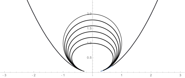
Figure 2. This shows the projective action of a one-dimensional parabolic group on ${\mathbb{S}}_{+}$ with boundary represented as a parabola. We use the affine patch where $x>0$ in the coordinate system. We normalize the homogeneous coordinates by setting $x=1$. The parabola $2z=y^{2}$ describes the boundary of ${\mathbb{S}}_{+}$ given by $y^{2}<2xz$. See Remark 3.2.

3.3.1. Parabolic regions

Let $g$ be a parabolic element with the expression (3.6) for $t>0$ under the parabolic coordinate system of Section 3.1.2. Assume that the Charette-Drumm invariant of $g$ is positive. That is, $\mu>0$ by Lemma 3.12. Recall from Section 3.1.2 that

$$F_{2}(x,y,z)=z^{2}-2\mu y\hbox{ and }F_{3}(x,y,z)=z^{3}-3\mu yz+3\mu^{2}x$$

are invariants of $g^{t}$. Recall that $\Phi(t):{\mathbf{E}}\rightarrow{\mathbf{E}}$ is generated by a vector field

$$\phi:=y\partial_{x}+z\partial_{y}+\mu\partial_{z}$$

with the square of the Lorentzian norm $\left|\mkern-2.0mu\left|\phi\right|\mkern-2.0mu\right|^{2}=z^{2}-2\mu y$.

The equation $F_{2}(x,y,z)=T$ gives us a parabolic cylinder $P_{T}$ in the $x$-direction with the parabola in the $yz$-plane. The vector field $\phi$ satisfies

$$\phi(x,y_{0},0)=(y_{0},0,\mu)\hbox{ for all }x\hbox{ and }T=-2\mu y_{0}.$$

Since we are looking for a $g^{t}$-invariant ruled surface, we take a line $l$ tangent to $P_{T}$ in the direction of $\mathbf{x}=(a,0,c)$ starting at $(0,y_{0},0)$. Since $\left(\mkern-4.0mu\left(\mathbf{x}\right)\mkern-4.0mu\right)\,\,\in{\mathbb{S}}_{+}$ by the premise, we obtain $2ac>0$ with $a>0,c>0$ under the parabolic coordinate system with the quadratic form (3.4). (See Figure 2.)

We define $\Psi(t,s)=g^{t}(l(s))$ so that

$$l(s)=(0,y_{0},0)+s(a,0,c)=(sa,y_{0},sc),\phi(l(s))=(y_{0},sc,\mu).$$

Thus, $\phi$ is never parallel to $(a,0,c)$ unless $s=0$. We choose $(a,0,c)$, $c\neq 0$, not parallel to $(y_{0},0,\mu)$, i.e.,

$$\frac{a}{c}\neq\frac{y_{0}}{\mu}.$$

Then $\phi|l$ is never parallel to the tangent vectors to $l$. Since $Dg^{t}(\phi)=\phi$, $\phi$ is never parallel to tangent vectors to $g^{t}(l)$, it follows that $\Psi$ is an immersion in $\mathsf{E}$.

Let $\mathcal{H}_{s_{0},\kappa_{1},\kappa_{2}}$ be the space of compact segments $u$ passing $\mathsf{E}$ with the following property:

• $u$ has an antipodal pair of endpoints in ${\mathbb{S}}_{+}$ and in the antipodal set ${\mathbb{S}}_{-}$ and

• $u\cap\mathsf{E}$ is equivalent under $g^{t}$ for some $t$ to a line $l(s)$ given by

  (3.13) $$l(s)=(sa,y_{0},sc)\hbox{ for }y_{0}\geq s_{0},a,c>0,\frac{\kappa_{1}a}{c}\leq\frac{y_{0}}{\mu}\leq\frac{\kappa_{2}a}{c},\hbox{ and }\\ a^{2}+c^{2}=1\hbox{ for some pair }0<\kappa_{1}\leq\kappa_{2}<1\hbox{ and }s_{0}>0.$$

This space has a metric coming from the Hausdorff metric ${\mathbf{d}}_{H}$.

We will prove the following in Appendix A.

Theorem 3.13.

Let $g$, $\mathcal{L}(g)\in{\mathsf{SO}}(2,1)^{o}$, be an accordant parabolic element acting properly on $\mathsf{E}$ with the positive Charette-Drumm invariant. Let $l$ be a line in $\mathcal{H}_{s_{0},\kappa_{1},\kappa_{2}}$ for the parabolic coordinate system for $g$. Then

• For each time-like line $l$ in the ruling of $S$,

  $$\{g^{t}({\rm Cl}(l))\}\rightarrow{\rm Cl}(\zeta_{{\mathbf{x}_{\infty}}})\hbox{ as }t\rightarrow\infty\hbox{ and }t\rightarrow-\infty$$

  geometrically.

• For any $\epsilon$-${\mathbf{d}}$-neighborhood $N$ of ${\rm Cl}(\zeta_{{\mathbf{x}_{\infty}}})\subset{\mathbb{S}}$, we can find such a ruled surface $S$ in $N\cap\mathsf{E}$.

• there exists a $\{g^{t},t\in{\mathbb{R}}\}$-invariant surface $S$ ruled by time-like lines containing $l^{o}$ properly embedded in $\mathsf{E}$ with boundary

  $${\rm Cl}(S)\setminus S=\{g^{t}({\mathbf{x}})|t\in{\mathbb{R}}\}\cup\{g^{t}({\mathbf{x}}_{-})|t\in{\mathbb{R}}\}\cup{\rm Cl}(\zeta_{{\mathbf{x}}_{\infty}})$$

  for a point ${\mathbf{x}}\in{\mathbb{S}}_{+}$, and ${\mathbf{x}}_{\infty}$ is a parabolic fixed point of $g$ in $\partial{\mathbb{S}}_{+}$ respectively. Furthermore, there exists a domain $R$ homeomorphic to a $3$-cell in $\mathsf{E}$ whose topological boundary in the hemisphere $\mathcal{H}$ equals ${\rm Cl}(S)$. Also, $R/\langle g\rangle$ is homeomorphic to a solid torus.

Definition 3.5.

In Theorem 3.13, the surface denoted by $S$ is called a parabolic ruled surface. (Compare with parabolic cylinders in Section 3.1.2.) The open region $R$ in $\mathsf{E}$ bounded by a parabolic ruled surface is called the parabolic region. The generator of the parabolic group acting on a parabolic ruled surface fixes a point $p\in\partial{\mathbb{S}}_{+}$.

An immersed image $S/\langle g\rangle$ of the surfaces in a manifold $\mathsf{E}/\Gamma$ is also called a parabolic ruled surface. The embedded image $R/\langle g\rangle$ of $R$ in a manifold $\mathsf{E}/\Gamma$ is called a parabolic region.

We can choose the parabolic surface and the parabolic regions so that they are in the $\epsilon$-${\mathbf{d}}$-neighborhood $N$ of $\bigcup_{x\in a}{{\rm Cl}(\zeta_{x})}\subset{\mathbb{S}}$ by the last item of Theorem 3.13. Then we call the parabolic region $\frac{1}{\epsilon}$-far away from the compact parts. The isometrically embedded images of such surfaces in $\mathsf{E}/\Gamma$ or $\mathsf{E}$ are described in the same manner.

3.3.2. Two transversal foliations

Figure 3. Three darker leaves of foliation $\mathcal{S}_{f,r_{0}}$ and five transversal light-gray leaves of $\mathcal{D}_{f,r_{0}}$ where $f(\rho)=\frac{3}{4}\frac{r}{\sqrt{1-r^{2}}}$ and $\mu=1$. See [10].

Assume

$$0<\kappa_{1}\leq\kappa_{2}<1.$$

Let $f:(0,1)\rightarrow{\mathbb{R}}$ be a strictly increasing smooth function satisfying

$$\kappa_{1}\mu\frac{r}{\sqrt{1-r^{2}}}\leq f(\rho)\leq\kappa_{2}\mu\frac{r}{\sqrt{1-r^{2}}}.$$

Let $\mathcal{H}_{f}$ be the space of compact segments $u$ passing $\mathsf{E}$ with the following property:

• $u$ has an antipodal pair of endpoints in ${\mathbb{S}}_{+}$ and in ${\mathbb{S}}_{-}$,

• $u\cap\mathsf{E}$ is equivalent under $g^{t}$ for some $t$ to a line $l(s)$ given by $l_{f,r}(s)=(sa,y_{f}(\rho),sc),s\in{\mathbb{R}}$, where

  $$y_{f}(\rho):=f(\rho),a=r,c=\sqrt{1-r^{2}},r\in(0,1).$$

For fixed $r\in(0,1)$, let $S_{f,r}$ denote the parabolic ruled surface given by

$$\bigcup_{t,s\in{\mathbb{R}}}g^{t}(l_{f,r}(s)).$$

Define $D_{f,r_{0},t}$ for fixed $t\in{\mathbb{R}}$ denote the surface

$$\bigcup_{s\in{\mathbb{R}},r\in[r_{0},1)}g^{t}(l_{f,r}(s)).$$

We will prove the following in Appendix A.

Theorem 3.14.

Let $r_{0}\in(0,1)$. Then the following hold:

• The surfaces $S_{f,r}$ for $r\in[r_{0},1)$ are properly embedded leaves of a foliation $\tilde{\mathcal{S}}_{f,r_{0}}$ of the region $R_{f,r_{0}}$, closed in $\mathsf{E}$, bounded by $S_{f,r_{0}}$ where $g^{t}$ acts on.

• $\{D_{f,r_{0},t},t\in{\mathbb{R}}\}$ is the set of properly embedded leaves of a foliation $\tilde{\mathcal{D}}_{f,r_{0}}$ of $R_{f,r_{0}}$ by disks meeting $S_{f,r}$ for each $r$, $r_{0}<r<1,$ transversally.

  • $g^{{t_{0}}}(D_{f,r_{0},t})=D_{f,r_{0},t+t_{0}}$.

  • $D_{f,r_{0},t^{\prime}}\cap D_{f,r_{0},t}=\emptyset$ for $t,t^{\prime},t\neq t^{\prime}$.

  • ${\rm Cl}(D_{f,r_{0},t})\cap{\mathbb{S}}_{+}$ is given as a geodesic ending at the parabolic fixed point of $g$.

Remark 3.3.

The quotient $R_{f,r_{0}}/\langle g\rangle$ is foliated by the foliation $\mathcal{S}_{f,r_{0}}$ induced by $\tilde{\mathcal{S}}_{f,r_{0}}$ and $\mathcal{D}_{f,r_{0}}$ induced by $\tilde{\mathcal{D}}_{f,r_{0}}$. The leaves of $\mathcal{S}_{f,r_{0}}$ are annuli of the form $S_{f,r}/\langle g\rangle$ and the leaves of $\mathcal{D}_{f,r_{0}}$ are the embedded images of $D_{f,r_{0},t}$ for $t\in{\mathbb{R}}$. The embedded image of $R_{f,r_{0}}/\langle g\rangle$ in $\mathsf{E}/\Gamma$ are foliated by induced foliations to be denoted by the same names.

4. Orbits of proper affine deformations and translation vectors

We now come to the most important section of this paper. In this section, we assume $\mathcal{L}(\Gamma)\subset{\mathsf{SO}}(2,1)^{o}$ and work with Criterion 1.1 only without assuming the properness of the $\Gamma$-action. In Sections 4.1 and 4.2, we will present the objects of our discussion. In Section 4.3, we will discuss the Anosov properties of geodesic flows extended to a flat bundle $\mathbf{V}$. In Section 4.4, we will put the translation cocycle into an integral form. In Section 4.5, we will compute the translation parts of the holonomy representations. Theorem 4.8 is the main result where we will give an outline of the proof. We will prove the converse part of Theorem 1.5 at the end of Section 4.5. In Section 4.6, we obtain Corollary 4.9 which discusses all the accumulation points of $\Gamma$.

4.1. Convergence sequences

Let $g\in\Gamma$. Let $\lambda_{1}(g)$ denote the largest eigenvalue of $\mathcal{L}(g)$, which has eigenvalues $\lambda_{1}(g),1,1/\lambda_{1}(g)$. Note the relation

(4.1) $${\color[rgb]{0,0,0}l_{{\mathbb{S}}_{+}}(g)}=\log\left(\frac{\lambda_{1}(g)}{1/\lambda_{1}(g)}\right)=2\log\lambda_{1}(g).$$

Recall that $\Gamma$ acts as a convergence group of a circle $\partial{\mathbb{S}}_{+}$. That is, if $g_{i}$ is a sequence of mutually distinct elements of $\Gamma$, then there exists a subsequence $g_{j_{i}}$ and points $a,r$ in $\partial{\mathbb{S}}_{+}$ so that

• as $i\rightarrow\infty$, $\{g_{j_{i}}|\partial{\mathbb{S}}_{+}\setminus\{r\}\}$ uniformly converges to a constant map with value $a$ on every compact subset, and

• as $i\rightarrow\infty$ $\{g_{j_{i}}^{{-1}}|\partial{\mathbb{S}}_{+}\setminus\{a\}\}$ uniformly converges to a constant map with value $r$ on every compact subset.

Call $a$ the attractor of $\{g_{j_{i}}\}$ and $r$ the repeller of $\{g_{j_{i}}\}$. Here, $a$ may or may not equal $r$. (See [1] for detail.) We call the sequence ${g_{i}}$ satisfying the above properties the convergence sequence.

For a point $x\in\mathsf{E}$, let $\Gamma(x)$ denote the orbit of $x$. We define the Lorentzian limit set $\Lambda_{\Gamma}:=\bigcup_{x\in\mathsf{E}}({\rm Cl}(\Gamma(x))\setminus\Gamma(x))$. By the properness of the action, we obviously have:

Lemma 4.1.

Let $\Gamma$ be a proper affine free group with rank $\geq 2$. Then $\Lambda_{\Gamma}$ is a subset of ${\mathbb{S}}$.

Recall ${\mathbb{S}}_{0}={\mathbb{S}}\setminus{\mathbb{S}}_{+}\setminus{\mathbb{S}}_{-}$. For each point $x$ of $\partial{\mathbb{S}}_{+}$, there exists an accordant great segment $\zeta_{x}$ (see Definition 3.3). We denote by $\Pi_{+}:{\mathbb{S}}_{0}\rightarrow\partial{\mathbb{S}}_{+}$ the map given by sending every point of ${\rm Cl}(\zeta_{x})$ to $x$. This is a fibration by Section 3.4 of [16].

Let $\Lambda_{\Gamma,{\mathbb{S}}_{+}}\subset{\rm Cl}({\mathbb{S}}_{+})$ be the limit set of the discrete faithful Fuchsian group action on ${\mathbb{S}}_{+}$ by $\mathcal{L}(\Gamma)$. (See [2].)

One of our main results of the section is Corollary 4.9 also giving us:

Theorem 4.2.

Let $\Gamma$ be a proper affine free group of rank $\geq 2$ with or without parabolics. Assume $\mathcal{L}(\Gamma)\subset{\mathsf{SO}}(2,1)^{o}$. Then $\Lambda_{\Gamma}\subset\Pi_{+}^{-1}(\Lambda_{\Gamma,{\mathbb{S}}_{+}}).$

4.2. The bundles ${\mathbf{E}}$ over $\mathsf{U}{\mathsf{S}}$

Let $\mathsf{U}{\mathbb{S}}_{+}$ denote the unit tangent bundle of ${\mathbb{S}}_{+}$, i.e., the space of direction vectors on ${\mathbb{S}}_{+}$. For any subset $A$ of ${\mathbb{S}}_{+}$, we let $\mathsf{U}A$ denote the inverse image of $A$ in $\mathsf{U}{\mathbb{S}}_{+}$ under the projection. The projection $\Pi_{{\mathsf{S}}}:\mathsf{U}{\mathsf{S}}\rightarrow{\mathsf{S}}$ lifts to the projection $\Pi_{{\mathbb{S}}_{+}}:\mathsf{U}{\mathbb{S}}_{+}\rightarrow{\mathbb{S}}_{+}$.

Let $\Gamma:=h_{u}(\pi_{1}({\mathsf{S}}))$ be a proper affine deformation free group of rank $\geq 2$. We note that $\Gamma$ acts on $\mathsf{U}{\mathbb{S}}_{+}$ as a deck transformation group over $\mathsf{U}{\mathsf{S}}$. An element $\gamma\in\Gamma$ goes to the differential map $D\gamma:\mathsf{U}{\mathbb{S}}_{+}\rightarrow\mathsf{U}{\mathbb{S}}_{+}$ defined by

$$D\gamma(x,\mathbf{u})=\left(\gamma(x),\left.\frac{d\gamma(\beta(t))}{dt}\right|_{t=0}\right),x\in{\mathbb{S}}_{+},\mathbf{u}\in\mathsf{U}_{x}{\mathbb{S}}_{+}$$

where $\beta(t)$ is a unit speed geodesic with $\beta(0)=x$ and $\dot{\beta}(0)=\mathbf{u}$. Goldman-Labourie-Margulis in [29] constructed a flat affine bundle ${\mathbf{E}}$ over the unit tangent bundle $\mathsf{U}{\mathsf{S}}$ of ${\mathsf{S}}$. They took the quotient of $\mathsf{U}{\mathbb{S}}_{+}\times\mathsf{E}$ by the diagonal action given by

$$\gamma(\mathbf{v},x)=(D\gamma(x),\gamma(\mathbf{v})),x\in\mathsf{U}{\mathbb{S}}_{+},\mathbf{v}\in\mathsf{E}$$

for a deck transformation $\gamma\in\Gamma$. The cover $\mathsf{U}{\mathbb{S}}_{+}\times\mathsf{E}$ of $\mathbf{E}$ is denoted by $\hat{\mathbf{E}}$ and is identical with $\mathsf{E}\times\mathsf{U}{\mathbb{S}}_{+}$. We denote by

$${\Pi_{\mathsf{E}}}:\hat{\mathbf{E}}=\mathsf{U}{\mathbb{S}}_{+}\times\mathsf{E}\rightarrow\mathsf{E}$$

the projection.

4.3. The Anosov property of the geodesic flow

We denote the standard $3$-vectors by

$$\mathbf{i}:=(1,0,0),\mathbf{j}=(0,1,0),\mathbf{k}=(0,0,1).$$

Definition 4.1.

We say that two positive-valued functions $f(t)$ and $g(t)$, $t\in{\mathbb{R}}$, are compatible or satisfy $f\cong g$ if there exists $C>1$ such that

$$\frac{1}{C}\leq\frac{f(t)}{g(t)}\leq C\hbox{ for }t\in{\mathbb{R}}.$$

Given $(\left(\mkern-4.0mu\left(\mathbf{x}\right)\mkern-4.0mu\right),{\mathbf{u}})\in\mathsf{U}{\mathbb{S}}_{+}$,

• we denote by $l(\left(\mkern-4.0mu\left(\mathbf{x}\right)\mkern-4.0mu\right),{\mathbf{u}})\subset{\mathbb{S}}_{+}$ the oriented complete geodesic passing through $\left(\mkern-4.0mu\left(\mathbf{x}\right)\mkern-4.0mu\right)$ in the direction of ${\mathbf{u}}$, and

• we denote by $\mathbf{v}_{+,(\left(\mkern-4.0mu\left(\mathbf{k}\right)\mkern-4.0mu\right),\mathbf{j})}$ and $\mathbf{v}_{-,(\left(\mkern-4.0mu\left(\mathbf{k}\right)\mkern-4.0mu\right),\mathbf{j})}$ the respective null vectors $\frac{1}{\sqrt{2}}\mathbf{j}+\frac{1}{\sqrt{2}}\mathbf{k}$ and $\frac{-1}{\sqrt{2}}\mathbf{j}+\frac{1}{\sqrt{2}}\mathbf{k}$ in the directions of the forward and backward endpoints of the oriented complete geodesic $l(\left(\mkern-4.0mu\left(\mathbf{k}\right)\mkern-4.0mu\right),\mathbf{j})\subset{\mathbb{S}}_{+}$.

• We define $\mathbf{v}_{+,(\left(\mkern-4.0mu\left(\mathbf{x}\right)\mkern-4.0mu\right),{\mathbf{u}})}$ and $\mathbf{v}_{-,(\left(\mkern-4.0mu\left(\mathbf{x}\right)\mkern-4.0mu\right),{\mathbf{u}})}$ respectively as the images of $\mathbf{v}_{+,(\left(\mkern-4.0mu\left(\mathbf{k}\right)\mkern-4.0mu\right),\mathbf{j})}$ and $\mathbf{v}_{-,(\left(\mkern-4.0mu\left(\mathbf{k}\right)\mkern-4.0mu\right),\mathbf{j})}$ under $g$ for $g\in{\mathsf{SO}}(2,1)^{o}$ provided

  $$g(\left(\mkern-4.0mu\left(\mathbf{k}\right)\mkern-4.0mu\right))=\left(\mkern-4.0mu\left(\mathbf{x}\right)\mkern-4.0mu\right)\hbox{ and }g(\mathbf{j})={\mathbf{u}}.$$

  The well-definedness of these objects follows since there is a one-to-one correspondence of $\mathsf{U}{\mathbb{S}}_{+}$ with ${\mathsf{SO}}(2,1)^{o}$.

Definition 4.2.

We define $\mathbf{V}$ as the quotient space of $\tilde{\mathbf{V}}:=\mathsf{U}{\mathbb{S}}_{+}\times{\mathbb{R}}^{2,1}$ under the diagonal action defined by

(4.2) $$\gamma(x,\mathbf{v})=(D\gamma(x),{\mathcal{L}}(\gamma)(\mathbf{v})),x\in\mathsf{U}{\mathbb{S}}_{+},\mathbf{v}\in{\mathbb{R}}^{2,1},\gamma\in\Gamma.$$

We will also need to define $\widetilde{\mathscr{V}}:={\mathbb{S}}_{+}\times{\mathbb{R}}^{2,1}$ and the quotient bundle $\mathscr{V}:=\widetilde{\mathscr{V}}/\Gamma$ where the action is given by

(4.3) $$\gamma(x,\mathbf{v})=(\gamma(x),{\mathcal{L}}(\gamma)(\mathbf{v})),x\in{\mathbb{S}}_{+},\mathbf{v}\in{\mathbb{R}}^{2,1},\gamma\in\Gamma.$$

The vector bundle $\mathbf{V}$ has a fiberwise Riemannian metric $\left|\mkern-2.0mu\left|\cdot\right|\mkern-2.0mu\right|_{\mathrm{fiber}}$ where $\Gamma$ acts as an isometry group. At $(\left(\mkern-4.0mu\left(\mathbf{x}\right)\mkern-4.0mu\right),{\mathbf{u}})\in\mathsf{U}{\mathbb{S}}_{+}$ with $\mathbf{x}\hbox{ satisfying }{\mathsf{B}}(\mathbf{x},\mathbf{x})=-1$, we give as a basis

(4.4) $$\left\{\mathbf{v}_{+,(\left(\mkern-4.0mu\left(\mathbf{x}\right)\mkern-4.0mu\right),{\mathbf{u}})},\mathbf{v}_{-,(\left(\mkern-4.0mu\left(\mathbf{x}\right)\mkern-4.0mu\right),{\mathbf{u}})},\mathbf{v}_{0,(\left(\mkern-4.0mu\left(\mathbf{x}\right)\mkern-4.0mu\right),{\mathbf{u}})}:=\frac{\mathbf{v}_{-,(\left(\mkern-4.0mu\left(\mathbf{x}\right)\mkern-4.0mu\right),{\mathbf{u}})}\times\mathbf{v}_{+,(\left(\mkern-4.0mu\left(\mathbf{x}\right)\mkern-4.0mu\right),{\mathbf{u}})}}{\left|\mkern-2.0mu\left|\mathbf{v}_{-,(\left(\mkern-4.0mu\left(\mathbf{x}\right)\mkern-4.0mu\right),{\mathbf{u}})}\times\mathbf{v}_{+,(\left(\mkern-4.0mu\left(\mathbf{x}\right)\mkern-4.0mu\right),{\mathbf{u}})}\right|\mkern-2.0mu\right|}\right\}$$

for the fiber over $\left(\mkern-4.0mu\left(\mathbf{x}\right)\mkern-4.0mu\right)$ where $\times$ is the Lorentzian cross product. We choose the positive definite metric $\left|\mkern-2.0mu\left|\cdot\right|\mkern-2.0mu\right|_{\mathrm{fiber}}$ on $\tilde{\mathbf{V}}$ so that the above vector frame is orthonormal at the fiber of $\tilde{\mathbf{V}}$ over $(\left(\mkern-4.0mu\left(\mathbf{x}\right)\mkern-4.0mu\right),{\mathbf{u}})$. The metric is ${\mathsf{SO}}(2,1)^{o}$-invariant on $\mathsf{U}{\mathbb{S}}_{+}$. Thus, this induces a metric $\left|\mkern-2.0mu\left|\cdot\right|\mkern-2.0mu\right|_{\mathrm{fiber}}$ on $\mathbf{V}$ as well.

Let $\tilde{\mathbf{V}}_{\omega}$ be the $1$-dimensional subbundle of $\mathsf{U}{\mathbb{S}}_{+}\times{\mathbb{R}}^{2,1}$ containing $\mathbf{v}_{\omega,(\left(\mkern-4.0mu\left(\mathbf{x}\right)\mkern-4.0mu\right),{\mathbf{u}})}$ for each $\omega$, $\omega=+,-,0$. It is redundant to say that $\mathbf{v}_{\omega,(\left(\mkern-4.0mu\left(\mathbf{x}\right)\mkern-4.0mu\right),{\mathbf{u}})}$ is a fiber over the point $\left(\mkern-4.0mu\left(\mathbf{x}\right)\mkern-4.0mu\right)$ in ${\mathbb{S}}_{+}$ for each $\omega$.

We define a so-called neutral map

$$\tilde{\mathbf{\nu}}:\mathsf{U}{\mathbb{S}}_{+}\rightarrow\mathsf{U}{\mathbb{S}}_{+}\times{\mathbb{R}}^{2,1}$$

given by $(\left(\mkern-4.0mu\left(\mathbf{x}\right)\mkern-4.0mu\right),{\mathbf{u}})\mapsto\mathbf{v}_{0,(\left(\mkern-4.0mu\left(\mathbf{x}\right)\mkern-4.0mu\right),{\mathbf{u}})}$. Here, $\tilde{\mathbf{\nu}}$ is an ${\mathsf{SO}}(2,1)^{o}$-equivariant map. By action of the isometry group $\Gamma$, we obtain a neutral section

$${\mathbf{\nu}}:\mathsf{U}{\mathsf{S}}\rightarrow{\mathbf{V}}$$

by using the ${\mathsf{SO}}(2,1)^{o}$-equivariance of the map. Hence, $\tilde{\mathbf{V}}_{0}$ coincides with the subspace generated by the image of the neutral section $\tilde{\mathbf{\nu}}$.

For any smooth map $g:\mathsf{U}{\mathbb{S}}_{+}\rightarrow\mathsf{U}{\mathbb{S}}_{+}$ or ${\mathbb{S}}_{+}\rightarrow{\mathbb{S}}_{+}$, we denote by ${\mathbb{D}}g$ the induced automorphism $\mathsf{U}{\mathbb{S}}_{+}\times\mathsf{E}$ acting trivially on the $\mathsf{E}$-factor.

Recall from Section 4.4 of [29] the geodesic flow $\Psi_{t}:\mathsf{U}{\mathbb{S}}_{+}\rightarrow\mathsf{U}{\mathbb{S}}_{+}$ denote the geodesic flow on $\mathsf{U}{\mathbb{S}}_{+}$ defined by the hyperbolic metric. Let

$${\mathbb{D}}\Psi_{t}:\mathsf{U}{\mathbb{S}}_{+}\times{\mathbb{R}}^{2,1}\rightarrow\mathsf{U}{\mathbb{S}}_{+}\times{\mathbb{R}}^{2,1}$$

denote the Goldman-Labourie-Margulis flow. This acts trivially on the second factor and as the geodesic flow on $\mathsf{U}{\mathbb{S}}_{+}$. The bundle $\mathbf{V}$ splits into three $\Psi_{t}$-invariant line bundles $\mathbf{V}_{+}$, $\mathbf{V}_{-}$ and $\mathbf{V}_{0}$, which are images of $\tilde{\mathbf{V}}_{+}$, $\tilde{\mathbf{V}}_{-}$ and $\tilde{\mathbf{V}}_{0}$. Our choice of $\left|\mkern-2.0mu\left|\cdot\right|\mkern-2.0mu\right|$ shows that ${\mathbb{D}}\Psi_{t}$ acts as uniform contractions in $\mathbf{V}_{+}$ as $t\rightarrow\infty,-\infty$, i.e.,

$$\left|\mkern-2.0mu\left|{\mathbb{D}}\Psi_{t}(\mathbf{v}_{+})\right|\mkern-2.0mu\right|_{\mathrm{fiber}}\cong\exp(-t)\left|\mkern-2.0mu\left|\mathbf{v}_{+}\right|\mkern-2.0mu\right|_{\mathrm{fiber}}\hbox{ for }\mathbf{v}_{+}\in\tilde{\mathbf{V}}_{+},$$

$$\left|\mkern-2.0mu\left|{\mathbb{D}}\Psi_{t}(\mathbf{v}_{-})\right|\mkern-2.0mu\right|_{\mathrm{fiber}}\cong\exp(t)\left|\mkern-2.0mu\left|\mathbf{v}_{-}\right|\mkern-2.0mu\right|_{\mathrm{fiber}}\hbox{ for }\mathbf{v}_{-}\in\tilde{\mathbf{V}}_{-},\hbox{ and }$$

(4.5) $$\left|\mkern-2.0mu\left|{\mathbb{D}}\Psi_{t}(\mathbf{v}_{0})\right|\mkern-2.0mu\right|_{\mathrm{fiber}}\cong\left|\mkern-2.0mu\left|\mathbf{v}_{0}\right|\mkern-2.0mu\right|_{\mathrm{fiber}}\hbox{ for }\mathbf{v}_{0}\in\tilde{\mathbf{V}}_{0}.$$

Here, $k$ in [29] equals $1$ since we can explicitly compute $k$ from the framing above. The signs are different from [29] because we have slightly different objects. The fiberwise metric on $\mathsf{U}{\mathbb{S}}_{+}$ is not dependent on the group $\Gamma$ itself. See the last paragraph of Section 4.4 of [29].

Figure 4. The frames on $\mathsf{U}{\mathbb{S}}_{+}$ and on $\mathsf{U}{\mathsf{S}}$. The circles bound horodisks covering the cusp neighborhoods below. The compact set $\mathscr{K}$ is some small compact set where the closed geodesics pass through. We drew only one closed geodesic.

Remark 4.1.

The induced geodesic flow on ${\mathsf{S}}$ is denoted by $\Psi_{t}$ and the induced action on $\mathbf{V}$ by ${\mathbb{D}}\Psi_{t}$. We may think of translating the picture of the flat bundle over $\mathsf{U}{\mathbb{S}}_{+}$ to the bundle over $\mathsf{U}{\mathsf{S}}$. As a bundle over $\mathsf{U}{\mathsf{S}}$, ${\mathbb{D}}\Psi_{t}$ contracts and expands uniformly for $\mathbf{V}_{\pm}$ with respect to $\left|\mkern-2.0mu\left|\cdot\right|\mkern-2.0mu\right|_{\mathrm{fiber}}$. However, in the picture over $\mathsf{U}{\mathbb{S}}_{+}$, ${\mathbb{D}}\Psi_{t}$ is the identity between fibers and objects lifted from $\mathbf{V}$ will uniformly increase or decrease exponentially with respect to any fixed Euclidean metric $\left|\mkern-2.0mu\left|\cdot\right|\mkern-2.0mu\right|_{E}$ on $\tilde{\mathbf{V}}$. (See Figure 4.)

Denote by

$$\widetilde{\mathbf{V}}_{+}(\left(\mkern-4.0mu\left(\vec{x}\right)\mkern-4.0mu\right),{\mathbf{u}}),\widetilde{\mathbf{V}}_{-}(\left(\mkern-4.0mu\left(\vec{x}\right)\mkern-4.0mu\right),{\mathbf{u}}),\widetilde{\mathbf{V}}_{0}(\left(\mkern-4.0mu\left(\vec{x}\right)\mkern-4.0mu\right),{\mathbf{u}})$$

the fibers of $\widetilde{\mathbf{V}}_{+},\widetilde{\mathbf{V}}_{-},\widetilde{\mathbf{V}}_{0}$ over $(\left(\mkern-4.0mu\left(\vec{x}\right)\mkern-4.0mu\right),{\mathbf{u}})\in\mathsf{U}{\mathsf{S}}$ respectively. We denote by

(4.6) $$\Pi_{\widetilde{\mathbf{V}}_{+}}:\widetilde{\mathbf{V}}\rightarrow\widetilde{\mathbf{V}}_{+},\Pi_{\widetilde{\mathbf{V}}_{-}}:\widetilde{\mathbf{V}}\rightarrow\widetilde{\mathbf{V}}_{-},\hbox{ and }\Pi_{\widetilde{\mathbf{V}}_{0}}:\widetilde{\mathbf{V}}\rightarrow\widetilde{\mathbf{V}}_{0}$$

the projections using the direct sum decomposition

$$\widetilde{\mathbf{V}}=\widetilde{\mathbf{V}}_{+}\oplus\widetilde{\mathbf{V}}_{-}\oplus\widetilde{\mathbf{V}}_{0}.$$

4.4. Computing translation vectors

Here, we will write the cocycle in terms of an integral. Let $g$ be a hyperbolic element. Let $a_{g}$ denote the attracting fixed point of $g$ in $\partial{\mathbb{S}}_{+}$ and $r_{g}$ the repelling one. Let $\Sigma_{+}$ denote the surface

$$(({\mathbb{S}}_{+}\cup\partial{\mathbb{S}}_{+})\setminus\Lambda_{\Gamma,{\mathbb{S}}_{+}})/\Gamma.$$

The surface ${\mathsf{S}}$ is the dense subset of $\Sigma_{+}$. The $\mathscr{V}$-valued forms are differential forms with values in the fiber spaces of $\mathscr{V}$. (See Definition 4.2.) The $\widetilde{\mathscr{V}}$-valued forms on ${\mathbb{S}}_{+}$ are simply the ${\mathbb{R}}^{2,1}$-valued forms on ${\mathbb{S}}_{+}$. However, the group $\Gamma$ acts by

(4.7) $$\gamma^{\ast}(\mathbf{v}\otimes dx)=\mathcal{L}(\gamma)^{-1}(\mathbf{v})\otimes d(x\circ\gamma)=\mathcal{L}(\gamma)^{-1}(\mathbf{v})\otimes\gamma^{*}dx,\gamma\in\Gamma.$$

(See Chapter 4 of Labourie [34].)

Let $\left|\mkern-2.0mu\left|\cdot\right|\mkern-2.0mu\right|_{E}$ denote a Euclidean metric on $\mathsf{E}$ by changing signs of the Lorentz metric which we fix from now on. Let $g$ be a hyperbolic isometry. Let $x_{g}$ be a point of the geodesic $l_{g}$ in ${\mathbb{S}}_{+}$ on which $g$ acts preserving an orientation direction $\mathbf{u}_{g}$. We define

$${\mathbf{\nu}}_{g}:=\mathbf{v}_{0,(x_{g},\mathbf{u}_{g})}=\tilde{\mathbf{\nu}}(x_{g},\mathbf{u}_{g}),$$

which is independent of the choice of $(x_{g},\mathbf{u}_{g})$ on $l_{g}$ by (4.4).

Recall from Section 3.2 the cocycle of $\Gamma=h_{\mathbf{b}}(\pi_{1}({\mathsf{S}}))$ for the holonomy homomorphism $h_{\mathbf{b}}$: $\mathbf{b}\in Z^{1}(\pi_{1}({\mathsf{S}}),{\mathbb{R}}^{2,1}_{h})$. We write every element $g$ as $g(x)=A_{g}x+\mathbf{b}_{g}$, $x\in\mathsf{E}$. Then the function $\mathbf{b}:\Gamma\rightarrow{\mathbb{R}}^{2,1}$ given by

$$g\mapsto\mathbf{b}_{g}\hbox{ for every }g$$

is a cocycle representing an element of

$$H^{1}(\pi_{1}({\mathsf{S}}),{\mathbb{R}}^{2,1})=H^{1}({\mathsf{S}},\mathscr{V})$$

using the de Rham isomorphism. (See Theorem 4.2.3 of Labourie [34].) Let $\eta$ denote the smooth $\mathscr{V}$-valued $1$-form on ${\mathsf{S}}$ representing the cocycle $\mathbf{b}$ in the de Rham sense.

Let $\tilde{\eta}:{\mathbb{S}}_{+}\rightarrow{\mathbb{R}}^{2,1}$ denote the lift of $\eta$ to ${\mathbb{S}}_{+}$. We can think of $\tilde{\eta}$, which is $h$-equivariant, as the differential of a section $s_{\tilde{\eta}}:{\mathbb{S}}_{+}\rightarrow\mathsf{E}$ which is $h_{\mathbf{b}}$-equivariant:

(4.8) $$\tilde{\eta}=ds_{\tilde{\eta}}$$

by Theorem 1.14 of [26] and lifting to the cover ${\mathbb{S}}_{+}\times\mathsf{E}$.

Recall from Section 2.2, the end neighborhood $E$ and its inverse image $\mathscr{H}\subset{\mathbb{S}}_{+}$. Let $\mathcal{CH}(\Lambda)$ denote the convex hull of a closed subset $\Lambda$ of $\partial{\mathbb{S}}_{+}$ in ${\mathbb{S}}_{+}$. The surface ${\mathsf{S}}_{C}:=\mathcal{CH}(\Lambda_{\Gamma,{\mathbb{S}}_{+}})/\Gamma$ is a finite-volume connected hyperbolic surface with geodesic boundary and cusp ends. The boundary of ${\mathsf{S}}_{C}$ is a union of finitely many closed geodesic boundary components, and each end of ${\mathsf{S}}_{C}$ is a cusp. Assume that each component of $E$ is a subset of ${\mathsf{S}}_{C}$ by choosing suitable cusp neighborhoods. We let $F$ to denote a compact fundamental domain of $\mathcal{CH}(\Lambda_{\Gamma,{\mathbb{S}}_{+}})\setminus{{\mathscr{H}}}$.

Let $\mathsf{U}{\mathsf{S}}_{C}$ denote the space of unit vectors on ${\mathsf{S}}$ with base points at ${\mathsf{S}}_{C}$, and $\mathsf{U}\mathcal{CH}(\Lambda_{\Gamma,{\mathbb{S}}_{+}})$ denote one for $\mathcal{CH}(\Lambda_{\Gamma,{\mathbb{S}}_{+}})$. We can compute the cocycle $\mathbf{b}$ by the following way:

Let $\mathscr{K}$ be a small fixed compact domain in $\mathcal{CH}(\Lambda_{\Gamma,{\mathbb{S}}_{+}})\setminus{\mathscr{H}}$ in ${\mathbb{S}}_{+}$. Let $\tilde{\eta}$ denote the lift of $\eta$ on ${\mathbb{S}}_{+}$. We may also assume that

(4.9) $$\tilde{\eta}|\mathscr{K}\equiv 0$$

by locally changing $\eta$ by (4.8). We simply need to change the section to a section that is a fixed parallel section on $p_{{\mathsf{S}}}(\mathscr{K})$. This can obviously be achieved by using a partition of unity while this does not change the cohomology class of $\eta$. (See Section 4 of [29].)

To simplify, we assume that $s_{\tilde{\eta}}$ at $\mathscr{K}$ takes the value of the origin $O$.

Definition 4.3.

Let $\Gamma_{\hat{K}}$ denote the set of hyperbolic elements $g\in\Gamma$ that acts on a geodesic $l_{g}$ in ${\mathbb{S}}_{+}$ passing a compact subset $\mathscr{K}\subset{\mathbb{S}}_{+}\setminus{\mathscr{H}}$.

We lift the discussion to $\mathsf{U}{\mathsf{S}}_{C}$ and its cover $\mathsf{U}\mathcal{CH}(\Lambda_{\Gamma,{\mathbb{S}}_{+}})\subset\mathsf{U}{\mathbb{S}}_{+}$. Let $g$ be an element of $\Gamma_{\mathscr{K}}$ corresponding to a closed geodesic $c_{g}$. Let $l_{g}$ be the unit speed geodesic in ${\mathbb{S}}_{+}$ in connecting $x_{g}\in\mathscr{K}$ to $g(x_{g})$ covering $c_{g}$ with the length $t_{g}$. Let $\Pi_{{\mathbb{R}}^{2,1}}:\mathsf{U}{\mathbb{S}}_{+}\times{\mathbb{R}}^{2,1}\rightarrow{\mathbb{R}}^{2,1}$ denote the projection to the second factor. Then by the trivialization on $\mathscr{K}$

(4.10) $$\mathbf{b}_{g}=\Pi_{{\mathbb{R}}^{2,1}}\left(\int_{[0,t_{0}]}\tilde{\eta}\left(\frac{dl_{g}(t)}{dt}\right)dt\right)$$

where $t_{g}$ is the time needed to go from $x_{g}$ to $g(x_{g})$. (See Section 4.2.2 of Labourie [34].) However, we will consider the case when $x_{g}$ is anywhere in ${\mathbb{S}}_{+}$, Since

(4.11) $$\Pi_{{\mathbb{R}}^{2,1}}\left(\int_{[0,t_{g}]}\tilde{\eta}\left(\frac{dl_{g}(t)}{dt}\right)dt\right)=g(\Pi_{\mathsf{E}}\circ s_{\tilde{\eta}}(x_{g})))-\Pi_{\mathsf{E}}\circ s_{\tilde{\eta}}(x_{g})\\ =(\mathcal{L}(g)-{\rm I})(\Pi_{\mathsf{E}}\circ s_{\tilde{\eta}}(x_{g}))+{\color[rgb]{0,0,0}\mathbf{b}_{g}},$$

we have

(4.12) $$\mathbf{b}_{g}=\Pi_{{\mathbb{R}}^{2,1}}\left(\int_{[0,t_{g}]}\tilde{\eta}\left(\frac{dl_{g}(t)}{dt}\right)dt\right)+({\rm I}-\mathcal{L}(g))({\Pi_{\mathsf{E}}\circ}s_{\tilde{\eta}}(x_{g})).$$

Thus, we obtain

(4.13) $$\mathbf{b}_{g}=\Pi_{{\mathbb{R}}^{2,1}}\Bigg{(}\int_{[0,t_{g}]}{\mathbb{D}}\Psi((x_{g},{\mathbf{u}}_{g}),t)^{-1}\left(\tilde{\eta}\left(\frac{d\Psi((x_{g},{\mathbf{u}}_{g}),t)}{dt}\right)\right)dt\Bigg{)}\\ +({\rm I}-\mathcal{L}(g))({\Pi_{\mathsf{E}}\circ}s_{\tilde{\eta}}(x_{g}))$$

where the geodesic segment $\Psi((x_{g},{\mathbf{u}}_{g}),[0,t_{g}])$ for a unit vector ${\mathbf{u}}_{g}$ at $x_{g}$, covers a closed curve representing $g$.

Using the origin $O$ of $\mathsf{E}$, we can consider it as ${\mathbb{V}}$ with a vector subspace ${\mathbb{V}}_{\omega}$, $\omega=+,-,0$. Define $\Pi_{\omega,x_{0}}:=\Pi_{{\mathbb{R}}^{2,1}}\circ\Pi_{\widetilde{\mathbf{V}}_{\omega},x_{0}}:\{x_{0}\}\times\mathsf{E}\rightarrow{\mathbb{V}}_{\omega,x_{0}}\rightarrow{\mathbb{R}}^{2,1}$ to denote the projection $\Pi_{\widetilde{\mathbf{V}}_{\omega}}$ at the fiber $\mathsf{E}$ over $x_{0}\in\mathsf{U}{\mathbb{S}}_{+}$. Define

(4.14) $$\tilde{\eta}_{\omega}(x_{0})=\Pi_{\widetilde{\mathbf{V}}_{\omega,x_{0}}}(\tilde{\eta}(x_{0})),$$

where $\omega=+,-,0$. Since $\Psi_{t}$ preserves the decomposition, ${\mathbb{D}}\Psi(x,t)$ commutes with these projections.

Definition 4.4.

Let $\mathscr{K}$ be the compact subset of ${\mathbb{S}}_{+}\setminus{\mathscr{H}}$. Let $g\in\Gamma_{\mathscr{K}}$. We choose $x_{g}\in\mathscr{K}$ so that the arc $\Psi((x_{g},{\mathbf{u}}_{g}),[0,t_{g}])$ for a unit vector ${\mathbf{u}}_{g}$ at $x_{g}$ covers a closed geodesic representing $g$ where $(g(x_{g}),Dg({\mathbf{u}}_{g}))=\Psi((x_{g},{\mathbf{u}}_{g}),t_{g})$. The arc here is not necessarily in $\mathscr{K}$ of course. We define invariants:

(4.15) $$\mathbf{b}_{g,\omega}:=\Pi_{\widetilde{\mathbf{V}}_{\omega},x_{g}}(\mathbf{b}_{g})=\\ \Pi_{{\mathbb{R}}^{2,1}}\Bigg{(}\int_{[0,t_{g}]}{\mathbb{D}}\Psi((x_{g},{\mathbf{u}}_{g}),t)^{-1}\left(\tilde{\eta}_{\omega}\left(\frac{d\Psi((x_{g},{\mathbf{u}}_{g}),t)}{dt}\right)\right)dt\Bigg{)}\\ +({\rm I}-\mathcal{L}(g))\left({\Pi_{\omega,x_{g}}}(s_{\tilde{\eta}}(x_{g}))\right),$$

where $\omega=+,-,0$ respectively. The second equalities hold since ${\mathbb{D}}\Psi(x,t)$ and $\mathcal{L}(g)$ commute with projections $\Pi_{\widetilde{\mathbf{V}}_{+}},\Pi_{\widetilde{\mathbf{V}}_{-}}$ and $\Pi_{\widetilde{\mathbf{V}}_{0}}$.

Proposition 4.3.

For nonparabolic $g\in\Gamma-\{{\rm I}\}$, we have

(4.16) $$\mathbf{b}_{g,0}=\alpha(g){\mathbf{\nu}}_{g},$$

(4.17) $$\left|\mkern-2.0mu\left|\mathbf{b}_{g,0}\right|\mkern-2.0mu\right|=\alpha(g).$$

Proof.

First, $\mathbf{b}_{g,0}$ is parallel to ${\mathbf{\nu}}_{g}$ by (4.15). Since ${\mathbf{\nu}}_{g}$ is Lorentz orthogonal to the subspace spanned by $\mathbf{v}_{+,(x_{g},\mathbf{u}_{g})}$ and $\mathbf{v}_{-,(x_{g},\mathbf{u}_{g})}$, the component $\mathbf{b}_{g,0}$ is the image $\mathbf{b}_{g}$ under the Lorentzian projection to ${\mathbf{\nu}}_{g}$. Since $\mathbf{b}_{g}=g(O)-O$ for the origin $O$ by our choice of the $\mathbf{E}$-section near (4.9), and $\left|\mkern-2.0mu\left|{\mathbf{\nu}}_{g}\right|\mkern-2.0mu\right|=1$, (3.10) and Criterion 1.1 imply the result. ∎

The norm of a $1$-form with values in ${\mathbb{V}}_{0}$ is given by the fiberwise norm of ${\mathbb{V}}_{0}$ and the norm of hyperbolic metric for the tangent bundle of ${\mathsf{S}}$. Finally, we will need:

Definition 4.5.

Let $K$ be a compact subset of ${\mathsf{S}}$, and let $\tilde{K}$ denote the inverse image of $K$ in ${\mathbb{S}}_{+}$. The neutral factor of $\eta|K$ is given as the maximum norm of $\tilde{\eta}_{0}$ on $\mathsf{U}\tilde{K}$.

4.5. Translation vectors have direction limits in ${\mathbb{S}}_{0}$

We aim to prove Theorem 4.8 from Section 4.5.1 to Section 4.5.4. Section 4.5.1 discusses the standard cusp $1$-forms and how to integrate along geodesics to obtain the Margulis invariants. Important Lemma 4.6 shows that long cusp geodesics can absorb many possibly negative perturbations during the argument that we will present. Section 4.5.2 outlines the proof of Theorem 4.8. In Section 4.5.3, we show $\alpha(g_{i})\rightarrow\infty$ and $\alpha(g_{i})/\left|\mkern-2.0mu\left|\mathbf{b}_{g_{i}}\right|\mkern-2.0mu\right|\rightarrow\infty$ if $l_{{\mathbb{S}}_{+}}(g_{i})\rightarrow\infty$. We will use the fact that a sequence converges to $+\infty$ if we can show that a subsequence of any subsequence converges to $+\infty$. Hence, we will start with a subsequence and keep taking subsequences to obtain one that converges to $+\infty$. In Section 4.5.4, we finish the proof of the theorem on the limit of direction vectors.

4.5.1. Cusp forms

A standard horodisk $D$ is an open disk bounded by a horocycle in ${\mathbb{S}}_{+}$ passing $\left(\mkern-4.0mu\left(\mathbf{k}\right)\mkern-4.0mu\right)$ and ending at the unique point $\left(\mkern-4.0mu\left(\mathbf{j}+\mathbf{k}\right)\mkern-4.0mu\right)$. We denote by $\partial_{h}D$ the horocycle ${\rm Cl}(D)\setminus(D\cup\{\left(\mkern-4.0mu\left(\mathbf{j}+\mathbf{k}\right)\mkern-4.0mu\right)\})$ for any horodisk $D$.

Let $D^{\prime}$ be a horodisk in ${\mathbb{S}}_{+}$. Let $\mathbf{p}$ denote a null-vector in the direction of $p\in{\rm Cl}(D^{\prime})\cap\partial{\mathbb{S}}_{+}$. Let us use an upper half-space model of the hyperbolic plane with the standard coordinates $x,y$ and $p$ corresponding to $\infty$. Then we may assume without loss of generality that $D^{\prime}$ is given by $y>1$.

Definition 4.6.

Let $g$ be an accordant parabolic transformation in $\Gamma$. Using the parabolic coordinates, let $g$ be of the form (3.6) for some $t>0$. Let $E^{\prime}$ be a cusp neighborhood covered by $D^{\prime}$ where $\langle g\rangle$ acts as the deck transformation group. On $D^{\prime}$, we can find a $\mathscr{V}$-valued $1$-form

(4.18) $$\mu(x^{2}/2,-x,1)dx$$

that is closed but not exact and is $g$-invariant by (4.7) with respect to a coordinate system adopted to $g$. We call such a form on $D^{\prime}$ and the induced one on $E^{\prime}$ standard cusp $1$-forms, $\mu>0$ is the cusp coefficient of $E^{\prime}$. (See [14] to check the form and the invariance.)

Here $\mu>0$ by Lemma 3.12 since $t>0$ under the assumption.

Let ${{\mathscr{H}}}_{j}\subset{\mathbb{S}}_{+},j=1,2,\dots$, denote the horodisks covering the components of $E$. Let $p_{j}$ denote the parabolic fixed point corresponding to ${{\mathscr{H}}}_{j}$. Each ${{\mathscr{H}}}_{j}$ has standard coordinates $x_{j},y_{j}$ from the upper half-space model of ${\mathbb{S}}_{+}$ where $p_{j}$ becomes $\infty$, and ${{\mathscr{H}}}_{j}$ is given by $y_{j}>1$.

Since ${\mathsf{S}}$ has finitely many cusps, we can choose horocyclic end neighborhoods with mutually disjoint closures. By taking even smaller ones, we may also assume that

(4.19) $$d_{{\mathbb{S}}_{+}}(g({{\mathscr{H}}}_{i}),k({{\mathscr{H}}}_{j}))>C^{\text{\eqref{eqn:distH}}}_{E},C^{\text{\eqref{eqn:distH}}}_{E}\geq{\color[rgb]{0,0,0}5/4},g,k\in\Gamma,i,j=1,\dots,m_{0}$$

whenever $g({{\mathscr{H}}}_{i})\neq k({{\mathscr{H}}}_{j})$ for some fixed constant $C^{\text{\eqref{eqn:distH}}}_{E}$ depending only on $E$.

There are only finitely many cusps in ${\mathsf{S}}_{C}$. Thus, we can choose finitely many cusps in each orbit class of cusps whose closures meet the fundamental domain $F$. We may denote these by ${{\mathscr{H}}}_{1},\dots,{{\mathscr{H}}}_{m_{0}}$ by reordering if necessary. We denote by $\mathbf{p}_{1},\dots,\mathbf{p}_{m_{0}}$ the corresponding null vectors. We choose a parabolic coordinate system for each ${{\mathscr{H}}}_{j}$ in the $\Gamma$-equivariant manner.

Recall from Section 3.2 the cocycle of $\Gamma=h_{\mathbf{b}}(\pi_{1}({\mathsf{S}}))$ for the holonomy homomorphism $h_{\mathbf{b}}$: $\mathbf{b}\in Z^{1}(\pi_{1}({\mathsf{S}}),{\mathbb{R}}^{2,1}_{h})$. For each $\gamma\in\pi_{1}({\mathsf{S}})$, $\mathbf{b}(\gamma)=h_{\mathbf{b}}(\gamma)(x_{0})-x_{0}$ for a basepoint $x_{0}$. For each peripheral element $\gamma$ in the boundary orientation, let $\hat{\gamma}$ denote the corresponding deck transformation. We choose an adopted parabolic coordinate system where $h(\hat{\gamma})$ is accordant. Let $E_{\gamma}$ be a component of $E$ corresponding to $\gamma$. Let $\gamma^{\prime}$ be the homotopy class in $E_{\gamma}$ of the simple closed curve $c_{\gamma^{\prime}}$ bounding $E_{\gamma}$ with a basepoint $x_{0,\gamma}$. If we choose a basepoint to be the origin of the coordinate system, we obtain a class $\mathbf{u}$ in $H^{1}(\langle\hat{\gamma}\rangle,{\mathbb{R}}^{2,1}_{\langle h(\hat{\gamma})\rangle})$. Let $\tilde{c}_{\gamma^{\prime}}$ denote the boundary horocycle corresponding to $\hat{\gamma}$. Using the partition of unity, we change the section $s_{\tilde{\eta}}$ associated with $\tilde{\eta}$ so that so that $s_{\tilde{\eta}}|\tilde{c}_{\gamma^{\prime}}$ is the orbit of the origin of the one-parameter group of parabolic affine transformations containing $h(\hat{\gamma})$. By (4.8), new $\eta$ is obtained in $E_{\gamma}$. Since the de Rham class $[\eta^{c}_{\mu}]\in H^{1}(E^{\prime},\mathcal{V})$ goes to $\mathbf{u}\in H^{1}(\langle\hat{\gamma}\rangle,{\mathbb{R}}^{2,1}_{\langle h(\hat{\gamma})\rangle})$, we obtain by Propositions B.1 and B.2:

Corollary 4.4.

Let ${\mathsf{S}}$, $\Gamma$, $P$, $E$, and $\gamma$ be as above. Then we may replace a closed $\mathscr{V}$-valued $1$-form $\eta$ on ${\mathsf{S}}$ with a cohomologous one $\eta^{\prime}$ so that $\eta^{\prime}|E^{\prime}$ for each component $E^{\prime}$ of $E$ is a standard cusp $1$-form in a parabolic coordinate system adopted to the accordant holonomy element following the boundary orientation.

We may choose the $1$-form $\eta$ representing the cohomology class so that $\tilde{\eta}$, its lift to ${\mathbb{S}}_{+}$, is a standard cusp $1$-form on ${{\mathscr{H}}}_{j}$. Let $\mu_{j}$ denote the cusp coefficients for each $j$, $j=1,2,\dots$, Since there are only finitely many cusps in ${\mathbb{S}}_{+}/\Gamma$, there are only finitely many values of the cusp coefficients. Let $\mu_{\text{min}}$ be the minimum of $\mu_{1},\mu_{2},\dots$, and let $\mu$ be the maximum of $\mu_{1},\mu_{2},\dots$.

Let $\left|\mkern-2.0mu\left|\cdot\right|\mkern-2.0mu\right|_{E}$ denote a Euclidean metric on $\mathsf{E}$ which we fix in this paper.

Lemma 4.5.

Let $\mathscr{K}$ be a compact subset of ${\mathbb{S}}_{+}\setminus{\mathscr{H}}$. Suppose $x\in\mathscr{K}$. Then the matrix $\mathscr{C}_{i}$ with columns

(4.20) $$\mathbf{v}_{+,(x,\mathbf{u})},\mathbf{v}_{0,(x,\mathbf{u})},\mathbf{v}_{-,(x,\mathbf{u})}\hbox{ for every }\mathbf{u}\in\mathsf{U}_{x}{\mathbb{S}}_{+}$$

is in a compact subset of ${\mathsf{GL}}(3,{\mathbb{R}})$ depending only on $\mathscr{K}$.

Proof.

There is a uniformly bounded element of ${\mathsf{SO}}(2,1)^{o}$ sending a complete geodesic $\overline{\left(\mkern-4.0mu\left(0,-1,1\right)\mkern-4.0mu\right)\left(\mkern-4.0mu\left(0,1,1\right)\mkern-4.0mu\right)}$ to $l_{g_{i}}$ and $\left(\mkern-4.0mu\left(1,0,0\right)\mkern-4.0mu\right)$ to $\left(\mkern-4.0mu\left({\mathbf{\nu}}_{g_{i}}\right)\mkern-4.0mu\right)$. From this and the way we define the frames in Section 4.3, the conclusion follows. ∎

Let $g$ be a hyperbolic element. We recall from (4.15) and (4.16),

(4.21) $$\alpha(g)=\left|\mkern-2.0mu\left|\mathbf{b}_{g,0}\right|\mkern-2.0mu\right|,\mathbf{b}_{g,0}=\Pi_{\widetilde{\mathbf{V}}_{0},x_{g}}(\mathbf{b}_{g})=\\ \Pi_{{\mathbb{R}}^{2,1}}\left(\left(\int_{[0,t_{g}]}{\mathsf{B}}\left(\nu_{x_{g},{\mathbf{u}}_{g}},\tilde{\eta}\left(\frac{d\Psi((x_{g},{\mathbf{u}}_{g}),t)}{dt}\right)\right)dt\right)\nu_{x_{g},{\mathbf{u}}_{g}}\right)$$

since $({\rm I}-\mathcal{L}(g))\left({\Pi_{\widetilde{\mathbf{V}}_{0},x_{g}}}(s_{\tilde{\eta}}(x_{g}))\right)=0$.

For any subinterval $\zeta$ in a cusp with the cusp coefficient $\mu$, we define $\alpha(\zeta)$ to be the corresponding part of the above integral from $t_{\zeta_{0}}$ and $t_{\zeta_{1}}$ for the corresponding arc-length parametrizing interval $[t_{\zeta_{0}},t_{\zeta_{1}}]$. Define $R(\zeta)$ as the radius of $\zeta$ in the upper half-space model where the horocycle is given by $y=1$. By Proposition B.4, and the compatibility (4.3), we can use

(4.22) $$\alpha(\zeta)=\mu\left(\frac{\pm\sqrt{2}\sqrt{R(\zeta)^{2}-1}}{R(\zeta)}+2R(\zeta)\sqrt{R(\zeta)^{2}-1})\right)$$

Definition 4.7.

We define $r(\zeta):=\sqrt{R(\zeta)^{2}-1}$, which equals $1/2$ times the absolute value of the difference of the $x$-coordinates of the endpoint of $\zeta$ in the upper half-space model where the horocycle is given by $y=1$. The horospherical length $h$ of a cusp neighborhood $E$ is the $d_{{\mathbb{S}}_{+}}$-length of $\partial E$. Note that if two maximal geodesics $\zeta$ and $\zeta^{\prime}$ in a cusp $E$ have the same endpoints, then $r(\zeta)$ and $r(\zeta^{\prime})$ differ by a half an integer times $h$.

One useful result is Theorem 4.6 of Heinze and Hof [31],

(4.23) $$r(\hat{\zeta})=\sinh\frac{1}{2}(l_{{\mathbb{S}}_{+}}(\hat{\zeta})).$$

From this, we can show that the difference of $x$-coordinates of the end points of an arc of length $l$ is $\leq 2\sinh(\frac{l}{2})$.

Heuristically, Lemma 4.6 states that the homotopy classes of maximal geodesics in a cusp neighborhood will give quadratic differnces in $\alpha$-values. In particular the item (ii) gives us the main estimations to absorb the negative contributions.

Lemma 4.6 (Large cusp radius).

Let $\zeta$ be a maximal geodesic in a cusp neighborhood $E^{\prime}$ with the standard cusp $1$-form and a cusp coefficient $\mu^{\prime}$. Let $h$ be the horospherical length of $E^{\prime}$. There exists a positive constant $R_{\text{c}}$, independent of $\mu^{\prime}$ but dependent on $h$ and $C$, which is defined below so that for any $R_{1}>R_{\text{c}}$ has the following properties:

• For the set of maximal geodesics in $E^{\prime}$, $r(\zeta^{\prime})\mapsto\alpha(\zeta^{\prime})$ for each $\zeta^{\prime}$ in it forms a strictly increasing positive function of $r(\zeta^{\prime})$ for $r(\zeta^{\prime})>R_{1}$.

• Let $\zeta$ and $\zeta^{\prime}$ be two maximal geodesics in $E$ with the same endpoint as $\zeta$ but in the different homotopy classes with respect to endpoints. For any constant $0\leq\eta_{0}<C$ with

  $$R-h/2<r(\zeta)<R<r(\zeta^{\prime})\hbox{ for }R>R_{1},$$

  we have

  $$\alpha(\zeta^{\prime})-\alpha(\zeta)-\mu^{\prime}\eta_{0}\geq 2C^{(4.6)}_{R_{1},C}\mu^{\prime}r(\zeta^{\prime})^{2}$$

  for a constant $C^{(4.6)}_{R_{1},C}>0$ depending only on $h,R_{1}$ and $C$.

Proof.

We choose a horoball $\tilde{E}^{\prime}$ covering $E^{\prime}$. Then we can compute $\alpha(\zeta)$ for a geodesic $\zeta$ by lifting $\zeta$ to $\tilde{E}^{\prime}$. (i) is straightforward.

For (ii), the last term of (4.22) dominates the absolute values of other terms and $\mu\eta$ for sufficiently large $R_{1}$: Using (4.22), the above term divided by $\mu^{\prime}$ is bounded below by

$$r(\zeta^{\prime})^{2}-r(\zeta)^{2}-\eta_{0}-2\sqrt{2}.$$

Since $(x-{\color[rgb]{0,0,0}h/2})/x$ is an increasing function of $x$, the supremum on $x\in(R,R{\color[rgb]{0,0,0}+}h/2)$ is $R/(R+h/2)$. Hence, $r(\zeta)<C_{R}r(\zeta^{\prime})$ for $C_{R}=R/(R+h/2)$ since the ratio $r(\zeta)/r(\zeta^{\prime})$ is less than $C_{R}$ for $r(\zeta^{\prime})\geq R+h/2$. Then $\alpha(\zeta^{\prime})-\alpha(\zeta)-\mu^{\prime}\eta_{0}$ divided by $\mu^{\prime}$ is bounded below by

(4.24) $$r(\zeta^{\prime})^{2}(1-C_{R}^{2})-C-2\sqrt{2}\geq(1-C_{R}^{2})\left(r(\zeta^{\prime})^{2}-\frac{C+2\sqrt{2}}{1-C_{R}^{2}}\right).$$

Let $f_{R}(x)$ denote the polynomial given by the right side with $x$ replacing $r(\zeta^{\prime})$. The largest root of $f_{R}(x)$ is smaller than

$$\sqrt{\frac{(R+h)(C+2\sqrt{2})}{h}}.$$

Since the function $R\mapsto R$ dominates any function given by the square root of the 1st order polynomial of $R$, there exists $R^{\prime}>h$ so that for $R>R^{\prime}$, we have

$${\color[rgb]{0,0,0}R>\sqrt{\frac{(R+h)(C+2\sqrt{2})}{h}}}\hbox{ which implies }f_{R}(x)>0\hbox{ for }x>R.$$

Define $c:=\frac{f_{R^{\prime}+1}(R^{\prime}+1)}{(R^{\prime}+1)^{2}}>0$. Then

$$f_{R^{\prime}+1}(x)\geq cx^{2}\hbox{ for }x\geq R^{\prime}+1$$

by an easy calculus argument. We take $R_{1}=R^{\prime}+1$, and $C^{(4.6)}_{R_{1},C}=c/2$. We can make $R_{1}$ as large as we wish to since we only need $c>0$.

∎

4.5.2. Summing up the contributions

Let $\{g_{i}\}$ be a sequence of elements in $\Gamma_{\mathscr{K}}$. We denote by $\hat{l}_{g_{i}}$ the lift of $l_{g_{i}}$ to $\mathsf{U}{\mathbb{S}}_{+}$ directed towards the attracting fixed point of $g_{i}$ in $\partial{\mathbb{S}}_{+}$.

Recalling (4.15), we estimate $\mathbf{b}_{g_{i},-}(x)$. We give an outline of the rest of the long proof of Theorem 4.8 starting from Section 4.5.2:

• First, we estimate the last term in the integral (4.15) for $\omega=-$.

• We estimate the contribution of $\eta|{\mathsf{S}}_{C}\setminus E$ of the integral (4.15) for $\omega=-$.

• We estimate the contribution of the arcs in ${\mathscr{H}}$

  • We estimate the contribution of the arc when it is put into a standard position.

  • We obtain the relationship of the contributions to the arc in the standard position and actual one by Lemma 4.7.

  • We estimate the comparisons of sizes by length.

• Then we sum these results to estimate the integral (4.15) for $\omega=-$.

• In Section 4.5.3, we show that $\alpha(g_{i})\rightarrow\infty$ and $\alpha(g_{i})/\left|\mkern-2.0mu\left|\mathbf{b}_{g_{i},-}\right|\mkern-2.0mu\right|\rightarrow\infty$ as $l_{{\mathbb{S}}_{+}}(g_{i})\rightarrow\infty$.

• Finally, we estimate the asymptotic direction as the last item in Section 4.5.4.

Let $(x,{\mathbf{u}})\in\mathsf{U}\mathscr{K}$. The arc $\Psi((x,{\mathbf{u}}),[0,t])$ is a geodesic passing $\mathsf{U}\mathscr{K}$. We choose $x_{i}\in\mathscr{K}\cap l_{g_{i}}$ for each $i$ and the unit vector ${\mathbf{u}}_{i}$ at $x_{i}$ in the direction of $\hat{l}_{g_{i}}$. We let $t_{g_{i}}>0$ be so that $\Psi((x_{i},{\mathbf{u}}_{i}),[0,t_{g_{i}}])\subset l_{g_{i}}$ corresponds to the closed geodesic corresponding to $g_{i}$.

Let $\mathsf{U}{\mathsf{S}}_{C}$ denote the unit tangent bundle over ${\mathsf{S}}_{C}$.

• We denote by ${{\mathscr{H}}}_{i,1},{{\mathscr{H}}}_{i,2},\dots$, the components of ${\mathscr{H}}$ meeting $\Pi_{{\mathbb{S}}_{+}}(\Psi(x_{i},\mathbf{u}_{i}),t))$ as $t$ increases.

• Let $\mathbf{p}_{i,j}dx_{i,j}$ denote $\tilde{\eta}|{{\mathscr{H}}}_{i,j}$ where $\left(\mkern-4.0mu\left(\mathbf{p}_{i,j}\right)\mkern-4.0mu\right)$ is the parabolic fixed point in the boundary of ${{\mathscr{H}}}_{i,j}$.

• Let $t_{i,j}$, $0<t_{i,j}<t_{g_{i}},$ be the time the geodesic $\Psi((x_{i},{\mathbf{u}}_{i}),t)$ enters $\mathsf{U}{{\mathscr{H}}}_{i,j}$, and $\hat{t}_{i,j}$ the time it leaves $\mathsf{U}{{\mathscr{H}}}_{i,j}$ for the first time after $t_{i,j}$.

• We denote $I_{i,j}=[t_{i,j},\hat{t}_{i,j}]$.

(I) We estimate $\left|\mkern-2.0mu\left|({\rm I}-\mathcal{L}(g_{i}))({\Pi_{-,x_{g}}}\circ s_{\tilde{\eta}}(x_{i}))\right|\mkern-2.0mu\right|_{E}$ for $g\in\Gamma_{\mathscr{K}}$ from (4.15): The matrix of $\mathcal{L}(g_{i})$ with the basis $\mathbf{v}_{+,(x_{i},\mathbf{u}_{i})},\mathbf{v}_{0,(x_{i},\mathbf{u}_{i})},\mathbf{v}_{-,(x_{i},\mathbf{u}_{i})}$ is a diagonal matrix with entries

$$\lambda_{1}(g_{i}),1,1/\lambda_{1}(g_{i}).$$

Hence, the above is given by

(4.25) $$\left|\mkern-2.0mu\left|\left(1-\frac{1}{\lambda_{1}(g_{i})}\right)({\Pi_{-,x_{g}}}\circ s_{\eta}(x_{i}))\right|\mkern-2.0mu\right|_{E}<C_{\mathscr{K}}$$

where we have a uniform constant $C_{\mathscr{K}}$ depending only on $\mathscr{K}$ by Lemma 4.5 and (4.1) since $\lambda_{1}({g_{i}})>1$ and $\left|\mkern-2.0mu\left|s_{\tilde{\eta}}\right|\mkern-2.0mu\right|_{E}|\mathscr{K}$ is bounded by a constant depending only on $\mathscr{K}$.

(II) Define

$$N({\mathsf{S}}_{C}\setminus E):=\max\{\left|\mkern-2.0mu\left|\eta({\mathbf{u}})\right|\mkern-2.0mu\right|_{\mathrm{fiber}}|{\mathbf{u}}\in\mathsf{U}{\mathsf{S}}_{C}\setminus E\}.$$

We have

(4.26) $$\bigg{|}\bigg{|}\int_{[0,t_{g_{i}}]\setminus\bigcup_{j}I_{i,j}}{\mathbb{D}}\Psi((x_{i},{\mathbf{u}}_{i}),t)^{-1}\left(\tilde{\eta}_{-}\left(\frac{d\Psi((x_{i},{\mathbf{u}}_{i}),t)}{dt}\right)\right)dt\bigg{|}\bigg{|}_{\mathrm{fiber}}<C_{1}$$

for $C_{1}<\infty$ by the second part of (4.3) applied to ${\mathbb{D}}\Psi((x_{i},{\mathbf{u}}_{i}),t)^{-1}$ and the integrability of the exponential function. Here, $C_{1}=C_{1}(N({\mathsf{S}}_{C}\setminus E))$ depends only on $N({\mathsf{S}}_{C}\setminus E)$.

Since these integrals have values in the fibers over $\mathscr{K}$, and $\left|\mkern-2.0mu\left|\cdot\right|\mkern-2.0mu\right|_{\mathrm{fiber}}$ and $\left|\mkern-2.0mu\left|\cdot\right|\mkern-2.0mu\right|_{E}$ are uniformly compatible over $\mathscr{K}$, we have

(4.27) $$\bigg{|}\bigg{|}\int_{[0,t_{g_{i}}]\setminus\bigcup_{j}I_{i,j}}{\mathbb{D}}\Psi((x_{i},{\mathbf{u}}_{i}),t)^{-1}\left(\tilde{\eta}_{-}\left(\frac{d\Psi((x_{i},{\mathbf{u}}_{i}),t)}{dt}\right)\right)dt\bigg{|}\bigg{|}_{E}<C_{2}$$

for $C_{2}<\infty$. (See Remark 4.1.) Hence, $C_{2}$ depends only on $\mathscr{K}$ and $N({\mathsf{S}}_{C}\setminus E)$. We write $C_{2}=C_{2}(\mathscr{K},N({\mathsf{S}}_{C}\setminus E))$.

(III) For each $I_{i,j}$, we define for the maximal geodesic segment in $l_{g_{i}}\cap{{\mathscr{H}}}_{i,j}$

$$\eta_{i,j} :=\Pi_{{\mathbb{S}}_{+}}\circ\Psi((x_{i},{\mathbf{u}}_{i}),I_{i,j})\subset{{\mathscr{H}}}_{i,j}\,\hbox{ and }$$

(4.28) $$\mathbf{b}_{g_{i},-}(\eta_{i,j}) :=\int_{I_{i,j}}{\mathbb{D}}\Psi((x_{i},{\mathbf{u}}_{i}),t)^{-1}\left(\tilde{\eta}_{-}\left(\frac{d\Psi((x_{i},{\mathbf{u}}_{i}),t)}{dt}\right)\right)dt.$$

We now estimate $\mathbf{b}_{g_{i},-}$ contributed by $I_{i,j}$ by looking at the situation of (4.32).

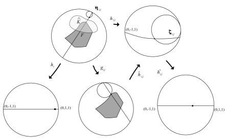
Figure 5. $g_{i,j}\in\Gamma$ moves $q_{i,j}$ to a point of $F$. $\hat{h}_{i,j}$ sends ${{\mathscr{H}}}_{i,j}$ to the standard horodisk $D$, $h_{i}$ is a normalization map of $l_{g_{i}}$, $h^{t}_{i,j}$ the normalization map for $h_{i,j}(l_{g_{i}})$, where $h_{ij}=\hat{h}_{ij}\circ g_{ij}$. See Definitions 4.8 and 4.9. The black dots indicate the images of $q_{i,j}$.

Recall the fundamental domain $F$ of $\mathcal{CH}(\Lambda_{\Gamma,{\mathbb{S}}_{+}})\setminus{{\mathscr{H}}}$ covering ${\mathsf{S}}_{C}\setminus E$. Let $p_{i}$ denote the beginning point in $\partial{\mathbb{S}}_{+}$ of $l_{g_{i}}$ in ${\mathbb{S}}_{+}$, and $p^{\prime}_{i}$ denote the forward endpoint of $l_{g_{i}}$ in $\partial{\mathbb{S}}_{+}$. Let $q_{i,j}$ denote the beginning point of $\eta_{i,j}$ itself and $\mathbf{u}_{i,j}$ the unit tangent vector to $l_{g_{i}}$ at the point $x_{i}$ in $\mathscr{K}$.

Definition 4.8.

We define three maps and two others slightly later.

$g_{i,j}$::

There is an element $g_{i,j}\in\Gamma$ so that $g_{i,j}(q_{i,j})\in F$, and

$$g_{i,j}({{\mathscr{H}}}_{i,j})={{\mathscr{H}}}_{k}\hbox{ for }k=1,\dots,m_{0}\hbox{ and }g_{i,j}(q_{i,j})\in F\cap{\rm Cl}({{\mathscr{H}}}_{k}).$$

$\hat{h}_{i,j}$::

Since $\{{{\mathscr{H}}}_{1},\dots,{{\mathscr{H}}}_{m_{0}}\}$ is finite, we can put ${{\mathscr{H}}}_{k}$ to the standard horodisk $D$ by a uniformly bounded sequence $h^{\prime}_{i,j}$ of elements of ${\mathsf{SO}}(2,1)^{o}$. Since $g_{i,j}(q_{i,j})$ is in a compact set $F\cap{\rm Cl}({{\mathscr{H}}}_{k})$, $h^{\prime}_{i,j}(g_{i,j}(q_{i,j}))$ is in a uniformly bounded subset of $\mathsf{U}\partial_{h}D$. Hence, we can put $h^{\prime}_{i,j}(g_{i,j}(p_{i}))$ to be $\left(\mkern-4.0mu\left(0,-1,1\right)\mkern-4.0mu\right)$ by a bounded sequence $h^{\prime\prime}_{i,j}$ of parabolic elements fixing $\left(\mkern-4.0mu\left(0,1,1\right)\mkern-4.0mu\right)$. Let $\hat{h}_{i,j}=h^{\prime\prime}_{i,j}\circ h^{\prime}_{i,j}$. Then

$$\hat{h}_{i,j}({\mathscr{H}}_{i,j})=D,\hat{h}_{i,j}(g_{i,j}(p_{i}))=\left(\mkern-4.0mu\left(0,-1,1\right)\mkern-4.0mu\right),$$

and $\hat{h}_{i,j}$ in a uniformly bounded set of elements of ${\mathsf{SO}}(2,1)^{o}$ not necessarily in $\Gamma$. This is called a normalization map. (There is a bound on the size of $\hat{h}_{i,j}$ depending only on $F$.)

$h_{i,j}$::

Let $h_{i,j}=\hat{h}_{i,j}\circ g_{i,j}$.

The image

$$\zeta_{i,j}=h_{i,j}(\eta_{i,j})$$

satisfies the premise of Lemma B.3. (See Figure 5.)

(III)(a) We define

(4.29) $$\mathbf{b}_{g_{i},-}(\zeta_{i,j}):=\\ \int_{I_{i,j}}{\mathbb{D}}\Psi(h_{i,j}(q_{i,j}),t-t_{i,j})^{-1}\left(h_{i,j}^{-1\ast}\tilde{\eta}_{-}\left(\frac{d\Psi(h_{i,j}(q_{i,j}),t-t_{i,j})}{dt}\right)\right)dt.$$

Proposition B.4 implies that

(4.30) $$\left|\mkern-2.0mu\left|\mathbf{b}_{g_{i},-}(\zeta_{i,j})\right|\mkern-2.0mu\right|_{E}\leq\mu_{k}r(\zeta_{i,j}).$$

Since there are only finitely many values of $\mu_{k}$s,

(4.31) $$\left|\mkern-2.0mu\left|\mathbf{b}_{g_{i},-}(\zeta_{i,j})\right|\mkern-2.0mu\right|_{E}\leq\mu r(\zeta_{i,j}).$$

(III)(b) We compute the actual contribution for $\eta_{i}$. We diagram the flow of the point $w\in\mathsf{U}{\mathbb{S}}_{+}$ and the action of the isometry $g$ not necessarily in $\Gamma$:

(4.32) $$\begin{CD}w@>{-t}>{}>\Psi(w,-t)\\ @V{}V{g}V@V{}V{g}V\\ g(w)@>{-t}>{}>\Psi(g(w),-t).\end{CD}$$

Lemma 4.7.

(4.33) $$\Pi_{{\mathbb{R}}^{2,1}}\left({\mathbb{D}}h_{i,j}^{-1}(\mathbf{b}_{g_{i},-}(\zeta_{i,j}))\right)=\Pi_{{\mathbb{R}}^{2,1}}\left(\mathbf{b}_{g_{i},-}(\eta_{i,j})\right).$$

Proof.

Since the flow commutes with isometry group action on $\mathsf{U}{\mathbb{S}}_{+}$, we have by considering (4.32) and the triviality of actions in the fibers

(4.34) $${\mathbb{D}}g({\mathbb{D}}\Psi(w,-t)(\mathbf{v}))=({\mathbb{D}}g\circ{\mathbb{D}}\Psi(w,-t)\circ{\mathbb{D}}g^{-1})\circ{\mathbb{D}}g(\mathbf{v})=\\ {\mathbb{D}}\Psi(g(w),-t)\circ{\mathbb{D}}g(\mathbf{v})\hbox{ for }w\in\mathsf{U}\mathscr{K},\mathbf{v}\in{\mathbb{R}}^{2,1},g\in{\mathsf{SO}}(2,1)^{o}.$$

We apply ${\mathbb{D}}h^{-1}_{i,j}$ to (4.29). Since $\Psi(x,t)^{-1}=\Psi(x,-t)$, we obtain by (4.34)

(4.35) $${\mathbb{D}}h_{i,j}^{-1}\left({\mathbb{D}}\Psi(h_{i,j}(q_{i,j},\mathbf{u}_{i,j}),t-t_{i,j})^{-1}\left(h_{i,j}^{-1\ast}\tilde{\eta}_{-}\left(\frac{d\Psi(h_{i,j}(q_{i,j},\mathbf{u}_{i,j}),t-t_{i,j})}{dt}\right)\right)\right)\\ ={\mathbb{D}}\Psi((q_{i,j},\mathbf{u}_{i,j}),t-t_{i,j})^{-1}{\mathbb{D}}h_{i,j}^{-1}\left(h_{i,j}^{-1\ast}\tilde{\eta}_{-}\left(\frac{d\Psi(h_{i,j}(q_{i,j},\mathbf{u}_{i,j}),t-t_{i,j})}{dt}\right)\right).$$

The above (4.35) equals by (4.7)

(4.36) $${\mathbb{D}}\Psi((q_{i,j},\mathbf{u}_{i,j}),t-t_{i,j})^{-1}{\mathbb{D}}h_{i,j}^{-1}\left(h_{i,j}^{-1\ast}\tilde{\eta}_{-}\left(\frac{d\Psi(h_{i,j}(q_{i,j},\mathbf{u}_{i,j}),t-t_{i,j})}{dt}\right)\right)\\ ={\mathbb{D}}\Psi((q_{i,j},\mathbf{u}_{i,j}),t-t_{i,j})^{-1}\left(\tilde{\eta}_{-}\left(Dh_{i,j}^{-1}\left(\frac{d\Psi(h_{i,j}(q_{i,j},\mathbf{u}_{i,j}),t-t_{i,j})}{dt}\right)\right)\right).$$

By the definition of differentials and (4.32), we obtain

(4.37) $$Dh_{i,j}^{-1}\left(\frac{d\Psi(h_{i,j}(q_{i,j},\mathbf{u}_{i,j}),t-t_{i,j})}{dt}\right)\\ =\frac{d(h_{i,j}^{-1}\circ\Psi)((h_{i,j}(q_{i,j},\mathbf{u}_{i,j}),t-t_{i,j})}{dt}=\frac{d\Psi((q_{i,j},\mathbf{u}_{i,j}),t-t_{i,j})}{dt}.$$

Above (4.36) equals by (4.37)

(4.38) $${\mathbb{D}}\Psi((q_{i,j},\mathbf{u}_{i,j}),t-t_{i,j})^{-1}\left(\tilde{\eta}_{-}\left(\frac{d\Psi((q_{i,j},\mathbf{u}_{i,j}),t-t_{i,j})}{dt}\right)\right).$$

Since $\Psi((x_{i},\mathbf{u}_{i}),t_{i,j})=(q_{i,j},\mathbf{u}_{i,j})$, (4.38) equals

(4.39) $${\mathbb{D}}\Psi(\Psi((x_{i},\mathbf{u}_{i}),t_{i,j}),t-t_{i,j})^{-1}\left(\tilde{\eta}_{-}\left(\frac{d\Psi(\Psi((x_{i},\mathbf{u}_{i}),t_{i,j}),t-t_{i,j})}{dt}\right)\right)\\ ={\mathbb{D}}\Psi((x_{i},\mathbf{u}_{i}),t)^{-1}\left(\tilde{\eta}_{-}\left(\frac{d\Psi((x_{i},\mathbf{u}_{i}),t)}{dt}\right)\right)\\ \hbox{ for every }t\in[t_{i,j},\hat{t}_{i,j}],(x_{i},\mathbf{u}_{i})\in\mathsf{U}\mathscr{K},$$

where we multiplied by ${\mathbb{D}}\Psi((x_{i},\mathbf{u}_{i}),t_{i,j})^{-1}$ which is ${\rm I}$ on the fibers to the left side. Integrating (4.35) and the last line of (4.39) for $[t_{i,j},\hat{t}_{i,j}]$, we proved (4.33). ∎

(III)(c) Now, we compare the contributions of these arcs. Now, $h_{i,j}(q_{i,j})\in\mathsf{U}\partial_{h}D$ is in a uniformly bounded subset $F^{\prime},\mathsf{U}F\subset F^{\prime}$, independent of $i,j$, of $\mathsf{U}{\mathbb{S}}_{+}$ since $h_{i,j}(p_{i})=\left(\mkern-4.0mu\left(0,-1,1\right)\mkern-4.0mu\right)$ and the complete geodesic containing $h_{i,j}(\eta_{i,j})$ passes the standard horodisk $D$.

Thus, $h_{i,j}(l_{g_{i}})$ is uniformly bounded from the line $\kappa$ in ${\mathbb{S}}_{+}$ connecting $\left(\mkern-4.0mu\left(0,-1,1\right)\mkern-4.0mu\right)$ to $\left(\mkern-4.0mu\left(\mathbf{j}+\mathbf{k}\right)\mkern-4.0mu\right)$, oriented towards $\left(\mkern-4.0mu\left(0,1,1\right)\mkern-4.0mu\right)$. Let $\hat{\kappa}$ denote the lift of $\kappa$ to $\mathsf{U}{\mathbb{S}}_{+}$ taking the direction towards $\left(\mkern-4.0mu\left(\mathbf{j}+\mathbf{k}\right)\mkern-4.0mu\right)$.

Definition 4.9.

We define two additional normalization maps:

$h^{\dagger}_{i,j}$::

We take a uniformly bounded element $h^{\dagger}_{i,j}$ of ${\mathsf{SO}}(2,1)^{o}$ so that $h^{\dagger}_{i,j}(h_{i,j}(l_{g_{i}}))=\kappa$ and $h^{\dagger}_{i,j}(h_{i,j}(q_{i,j}))=\left(\mkern-4.0mu\left(0,0,1\right)\mkern-4.0mu\right)$.

$h_{i}$::

Since $l_{g_{i}}$ is a geodesic passing $\mathscr{K}$, we take a uniformly bounded element $h_{i}$ of ${\mathsf{SO}}(2,1)^{o}$ so that $h_{i}(l_{g_{i}})=\kappa$ and $h_{i}(x_{i})=\left(\mkern-4.0mu\left(0,0,1\right)\mkern-4.0mu\right)$ without changing the orientation. (The bound only depends on $\mathscr{K}$.)

Then

$$h_{i}\circ h_{i,j}^{-1}\circ h^{\dagger,-1}_{i,j}(h^{\dagger}_{i,j}(\zeta_{i,j}))=h_{i}(\eta_{i,j})$$

and $h_{i}\circ h_{i,j}^{-1}\circ h^{\dagger,-1}_{i,j}$ acts on $\kappa$.

• Under $h_{i}\circ h_{i,j}^{-1}\circ h^{\dagger,-1}_{i,j}$, $h^{\dagger}_{i,j}\circ h_{i,j}(q_{i,j})$ goes to a point $h_{i}(q_{i,j})$.

• (4.40) $$d_{{\mathbb{S}}_{+}}(h^{\dagger}_{i,j}\circ h_{i,j}(q_{i,j}),h_{i}(q_{i,j}))=t_{i,j}$$

  since $h_{i}(x_{i})=\left(\mkern-4.0mu\left(0,0,1\right)\mkern-4.0mu\right)=h^{\dagger}_{i,j}\circ h_{i,j}(q_{i,j})$ and the $d_{{\mathbb{S}}_{+}}$-length of the arc from $x_{i}$ to $q_{i,j}$ is $t_{i,j}$ which is also the $d_{{\mathbb{S}}_{+}}$-length of the arc from $h_{i}(x_{i})$ to $h_{i}(q_{i,j})$.

By (4.1) and (4.40), the eigenvalue of $\mathcal{L}(h_{i}\circ h_{i,j}^{-1}\circ h^{\dagger,-1}_{i,j})$ at the eigenvector $(0,1,-1)$ is $\exp(-t_{i,j}/2)$. Since

$$\Pi_{{\mathbb{R}}^{2,1}}(\mathbf{b}_{g_{i},-}(\eta_{i,j}))=\Pi_{{\mathbb{R}}^{2,1}}(h_{i,j}^{-1\ast}(\mathbf{b}_{g_{i},-}(\zeta_{i,j}))),$$

$\mathcal{L}(h_{i}\circ h_{i,j}^{-1}\circ h^{\dagger,-1}_{i,j})$ sends the ${\mathbb{R}}^{2,1}$-vector

$$\Pi_{{\mathbb{R}}^{2,1}}(\mathcal{L}(h^{\dagger}_{i,j})(\mathbf{b}_{g_{i},-}(\zeta_{i,j})))\in\langle(0,-1,1)\rangle\hbox{ to }\Pi_{{\mathbb{R}}^{2,1}}(\mathcal{L}(h_{i})(\mathbf{b}_{g_{i},-}(\eta_{i,j})))\in\langle(0,-1,1)\rangle$$

by multiplying by $\exp(-t_{i,j}/2)$. Since $h^{\dagger}_{i,j}$ and $h_{i}$ are uniformly bounded depending only on $\mathscr{K}$ and $F$, we obtain

(4.41) $$\tilde{C}(F,\mathscr{K})\exp(-t_{i,j}/2)\left|\mkern-2.0mu\left|\mathbf{b}_{g_{i},-}(\zeta_{i,j})\right|\mkern-2.0mu\right|_{E}\geq\left|\mkern-2.0mu\left|\mathbf{b}_{g_{i},-}(\eta_{i,j})\right|\mkern-2.0mu\right|_{E}.$$

for a constant $\tilde{C}(F,\mathscr{K})>0$ depending only on $\mathscr{K}$ and $F$.

(IV) We sum up the contributions. Hence, $\frac{1}{R(\zeta_{i,j})}<1$. By (4.25), (4.27), (4.31), (4.41) and Proposition B.4, we estimate the upper bound depending only on $E,\mathscr{K},\eta|{\mathsf{S}}_{C}\setminus E$:

(4.42) $$\left|\mkern-2.0mu\left|\mathbf{b}_{g_{i},-}\right|\mkern-2.0mu\right|_{E}\leq\tilde{C}(F,\mathscr{K})\sum^{m_{i}}_{j}\exp(-t_{i,j}/2){\color[rgb]{0,0,0}\left(\mu\frac{r(\zeta_{i,j})(1+4R(\zeta_{i,j})^{2})}{2\sqrt{2}R(\zeta_{i,j})^{2}}\right)}\\ +C_{2}(\mathscr{K},N({\mathsf{S}}_{C}\setminus E))+C_{\mathscr{K}}\\ \leq\tilde{C}(F,\mathscr{K})\sum_{j}^{m_{i}}\exp(-t_{i,j}/2){\color[rgb]{0,0,0}\left(4\mu r(\zeta_{i,j})\right)}\\ +C_{2}(\mathscr{K},N({\mathsf{S}}_{C}\setminus E))+C_{\mathscr{K}}$$

since $R(\zeta_{ij})\geq 1$.

4.5.3. $\alpha(g_{i})\rightarrow\infty$ and $\frac{\alpha(g_{i})}{\left|\mkern-2.0mu\left|\mathbf{b}_{g_{i},-}\right|\mkern-2.0mu\right|}\rightarrow\infty$.

In Step (V), we will prove that $\alpha(g_{i})\rightarrow\infty$ and $\alpha(g_{i})/\left|\mkern-2.0mu\left|\mathbf{b}_{g_{i},-}\right|\mkern-2.0mu\right|\rightarrow+\infty$ provided $l_{{\mathbb{S}}_{+}}(g_{i})\rightarrow\infty$ using the fact that we can absorb many negative uncertainties during perturbation into long edges in the cusps using Lemma 4.6.

We can do this by showing that every subsequence has a subsequence converging to $+\infty$. We give an outline of the step (V).

• First, we will choose some constants such as $\epsilon,\delta,R_{0}$ sufficiently small or large.

• Let $g_{i}$ denote a closed geodesic. We replace the maximal segment $\zeta$ in a cusp neighborhood with $r(\zeta)>R_{0}+h/2$ with one $\zeta^{\prime}$ with the same endpoints but with $R_{0}<r(\zeta^{\prime})\leq R_{0}+h/2$. We denote the result by $\tilde{g}_{i}$.

• Then we find a closed geodesic $\hat{g}_{i}$ freely homotopic to $\tilde{g}_{i}$. Then we estimate $|\alpha(\tilde{g}_{i})-\alpha(\hat{g}_{i})|$ in terms of the constant times the number of components of the above arcs in (4.48). This constant is bounded since $R_{0}\delta=2$ by our choice below.

• This is the final step. $\alpha(g_{i})$ is bounded below by $\alpha(\hat{g}_{i})$ plus constant times the sum of $r(\zeta)^{2}$. Then we use the standard Schwartz inequalities.

Definition 4.10.

Let $g_{i}$ also denote the arclength-parameterized closed geodesic in ${\mathsf{S}}$ whose lift $l_{g_{i}}$ passes a fixed compact set $\mathcal{K}$ in ${\mathbb{S}}_{+}$. Let $J$ be the index set of mutually disjoint subintervals $I_{i}\subset I$ and $\alpha_{i}:=g_{i}|I_{i}$, By $g_{i}\setminus\bigcup_{i\in J}\alpha_{i}$, we mean the map $g_{i}|I\setminus\bigcup_{i\in I}I_{i}$.

We denote by $E_{\epsilon}$ the set obtained by decreasing $E$ inward by $\epsilon$ when $\epsilon>0$ and the $(-\epsilon)$-neighborhood of $E$ when $\epsilon<0$. We will assume that $E_{-1/2}$ is still a cusp-neighborhood, and $\eta|E_{-1/2}$ is still standard cusp $1$-form for each component by taking sufficiently smaller $E$ if necessary.

We denote by $\mu_{i,j}$ the cusp coefficient for the cusp neighborhood that $\zeta_{i,j}$ goes into. There are only finitely many values. We assume that the horospherical lengths of all cusp neighborhood components of $E$ equal $h$. Let $C_{{\mathsf{S}}\setminus E}$ denote the neutral factor of the compact set ${\mathsf{S}}\setminus E$.

We remark that following constants depend only on the two constants $h$ and $C_{{\mathsf{S}}\setminus E_{1}}$. There is no obstruction for the following choices.

(i) The first step is to decide on constants to be used later:

• Choose $\delta>0$ so that $0<\delta<1/40$ by Lemma 2.2 and let $\epsilon=7\delta$.

• We also require $\delta<\mu/(7C_{{\mathsf{S}}\setminus E_{1}})$.

• Also assume $6h\epsilon<1$, $\epsilon<1/8$, and $R_{0}>10$.

• We require $\delta$ to be given by $\delta:=2/R_{0}$ by taking $R_{0}$ sufficiently large and $\delta$ sufficiently small. By Lemma 2.3, the angle that $\zeta_{i,j}$ with $r(\zeta_{i,j})\geq R_{0}$ makes with the vertical line is $<\delta$ in the upper half-space model.

• $R_{0}$ is a constant satisfying all conclusions for the variable $R_{1}$ in Lemma 4.6 for $C>222\frac{\mu}{\mu_{\min}}$. For simplicity, we assume $R_{0}>10$.

(ii) We will replace very long $\zeta_{i,j}$ in $g_{i}$ with ones that are outside some cusp neighborhood: We denote by $\zeta_{i,j}$ the sequence of maximal geodesics in $g_{i}$ going into $E$. We denote by $J_{i,t}$ the set of $\zeta_{i,j}$ with $r(\zeta_{i,j})>t$ for $t\geq 0$.

For each $\zeta_{i,j}$ in $J_{i,R_{0}+h/2}$, we take a maximal geodesic $\hat{\zeta}_{i,j}$ with the same endpoints but with $R_{0}\leq r(\hat{\zeta}_{i,j})<R_{0}+h/2$ since we can decrease the $r(\zeta)$-values by $h/2$ times integers by wrapping a smaller number of times around the cusps. Since the geodesics are unique up to homotopy classes relative to endpoints, the homotopy class of $\hat{\zeta}_{i,j}$ is, of course, different from $\zeta_{i,j}$ relative to the endpoints. Thus, we obtain for $\zeta_{i,j}\in J_{i,R_{0}+h/2}$,

(4.43) $$\alpha(\zeta_{i,j})-\alpha(\hat{\zeta}_{i,j})\geq\mu_{i,j}\delta(R_{0}+h/2),\\ \alpha(\zeta_{i,j})-\alpha(\hat{\zeta}_{i,j})-\mu_{i,j}\eta_{0}\geq C^{(4.6)}_{R_{0}+h/2,C^{\prime}}\mu_{i,j}r(\zeta_{i,j})^{2},C^{(4,6)}_{R_{0}+h/2,C^{\prime}}>0$$

by Lemma 4.6 where $\eta_{0}<C^{\prime}$.

(iii) The third step is to estimate the relationship between $\alpha$-values for $g_{i}$ and the closed curves $\hat{g}_{i}$ and $\tilde{g}_{i}$ to be constructed: Let $\hat{g}_{i}$ denote the closed curve obtained by $g_{i}$ removing $\zeta_{i,j}$ and adding $\hat{\zeta}_{i,j}$ for each $\zeta_{i,j}\in J_{i,R_{0}+h/2}$. By Lemma 2.3, $\hat{g}_{i}$ has turning angles $<\delta=2/R_{0}$ at each endpoint of maximal geodesic segments by Lemma 2.3. We define

$$\hat{\alpha}(\hat{g}_{i}):=\alpha\left(g_{i}\setminus\bigcup_{\zeta\in J_{i,R_{0}+h/2}}\zeta\right)+\sum_{\zeta\in J_{i,R_{0}+h/2}}\alpha(\hat{\zeta}).$$

There exists a closed geodesic $\tilde{g}_{i}$ homotopic to $\hat{g}_{i}$ which is in the $\epsilon$-neighborhood of $\tilde{g}_{i}$ for $\epsilon=7\delta$ by Lemma 2.2. Let $E_{R_{0}/2+h/4+\epsilon}$ denote the cusp neighborhood obtained by moving $E$ inside by $R_{0}/2+h/4+\epsilon$. Then both $\hat{g}_{i}$ and $\tilde{g}_{i}$ are in ${\mathsf{S}}\setminus E_{R_{0}/2+h/4+\epsilon}$.

Define $\hat{J}_{i,0}$ the subset of $J_{i,0}$ of consisting of arcs $\zeta_{i,j}$ where where $d_{{\mathbb{S}}_{+}}$-lengths are strictly bigger than $5/4$. For every arc in $J_{i,0}\setminus\hat{J}_{i,0}$, the arcs are in ${\mathsf{S}}\setminus E_{5/8}$. We will not remove these from $g_{i}$ in the following because of this. By skipping these, we have

(4.44) $$|\hat{t}_{i,j}-t_{i,j}|\geq 5/4,|t_{i,j+1}-\hat{t}_{i,j}|\geq C^{\text{\eqref{eqn:distH}}}_{E}\geq 5/4\hbox{ for every }\zeta_{i,j}\in\hat{J}_{i,0}$$

where $C^{\text{\eqref{eqn:distH}}}_{E}$ is from (4.19).

Each maximal geodesic $\zeta_{i,j}\in\hat{J}_{i,0}\setminus J_{i,R_{0}+h/2}$ in $E$ of $g_{i}$ goes to a geodesic $\tilde{\zeta}_{i,j}$ in $E_{-1/8}$ of $\tilde{g}_{i}$ by the perpendicular projection which moves points by distances $<\epsilon<1/8$. We obtain two distances

$$d_{i,j,\pm}:=d_{{\mathbb{S}}_{+}}(\partial_{\pm}\zeta_{i,j},\partial_{\pm}\tilde{\zeta}_{i,j}).$$

These are less than $\epsilon$ by Lemma 2.1 since each endpoint of $\zeta_{i,j}\in J_{i,R_{0}+h/2}$ moves less than $\epsilon$. The corresponding endpoints are at most distance $d_{i,j,\pm}$ apart, which are values of the divergence functions corresponding to $\hat{t}_{i,j}$ and $t_{i,j}$ respectively. Hence, their $x$-coordinate values differ by less than ${\color[rgb]{0,0,0}1.1}d_{i,j,\pm}$ respectively using (4.23) as $0<\epsilon<1/8$. By last parts of [12] and [13] of the differences in the $\alpha$-values, we can estimate for $\zeta_{i,j}\in\hat{J}_{i,0}\setminus J_{i,R_{0}+h/2}$,

(4.45) $$|\alpha(\tilde{\zeta}_{i,j})-\alpha(\zeta_{i,j})|\leq 5\mu_{i,j}({\color[rgb]{0,0,0}R_{0}+h/2})(d_{i,j,+}/2+d_{i,j,-}/2)$$

since we can put in the new $x$-coordinates and take differences in $E_{-1/2}$ where $\eta$ has the form of the standard cusp $1$-form. Here, we need to use the fact that $r>10,\epsilon<1/8,\epsilon<r/80$, $r\mapsto\sqrt{r^{2}+1},r>0,$ is distance decreasing, and estimates of differences of the inverses of radii of arcs using calculus.

We claim that the sum of $d_{i,j,+}+d_{i,j,-}$ for $\zeta_{i,j}\in\hat{J}_{i,0}$ in $\tilde{g}_{i}\setminus\bigcup_{\zeta_{i,j}\in J_{i,R_{0}+h/2}}\tilde{\zeta}_{i,j}$ is less than $2$ times the sum of $d_{i,j,+}$ and $d_{i,j,-}$ over all $\zeta_{i,j}\in J_{i,R_{0}+h/2}$ which is less than $4\epsilon|J_{i,R_{0}+h/2}|$: We move $g_{i}\setminus\bigcup_{\zeta_{i,j}\in J_{i,R_{0}+h/2}}\zeta_{i,j}$ to $\tilde{g}_{i}\setminus\bigcup_{\zeta_{i,j}\in J_{i,R_{0}+h/2}}\tilde{\zeta}_{i,j}$ by perpendicular projections, and hence, the endpoints of $\zeta_{i,j}$ for $\zeta_{i,j}\in J_{i,R_{0}+h/2}$ moving to $\tilde{\zeta}_{i,j}$ gives us the divergence functions. The sum of the values of the divergence functions at $t_{i,j},\hat{t}_{i,j}$ for the endpoints of $\zeta_{i,j}\in\hat{J}_{i,0}\setminus J_{i,R_{0}+h/2}$ in a component of $g_{i}\setminus\bigcup_{\zeta\in J_{i,R_{0}+h/2}}\zeta$, is less than $2$ times the sum of the values of its endpoints by (4.44) and Lemma 2.1.

Since each endpoint of $\zeta_{i,j}\in J_{i,R_{0}+h/2}$ moves less than $\epsilon$, we have by (4.45)

(4.46) $$\sum_{\zeta_{i,j}\in\hat{J}_{i,0}\setminus J_{i,R_{0}+h/2}}|\alpha(\tilde{\zeta}_{i,j})-\alpha(\zeta_{i,j})|\leq{\color[rgb]{0,0,0}10}\mu({\color[rgb]{0,0,0}R_{0}+h/2})\epsilon|J_{i,R_{0}+h/2}|.$$

As in the third paragraph above, for arcs $\hat{\zeta}_{i,j}\in J_{i,R_{0}+h/2}$, we have

$$|\alpha(\tilde{\zeta}_{i,j})-\alpha(\hat{\zeta}_{i,j})|\leq 5\mu({\color[rgb]{0,0,0}R_{0}+h/2})\epsilon.$$

Hence,

(4.47) $$\sum_{\zeta_{i,j}\in J_{i,R_{0}+h/2}}|\alpha(\tilde{\zeta}_{i,j})-\alpha(\hat{\zeta}_{i,j})|\leq 5\mu({\color[rgb]{0,0,0}R_{0}+h/2})\epsilon|J_{i,R_{0}+h/2}|.$$

For $\alpha$-values outside these, we integrate $\eta$ projected to the neutral bundle over

$$g_{i}\setminus\bigcup_{\zeta_{i,j}\in\hat{J}_{i,0}}\zeta_{i,j},\hbox{ and }\tilde{g}_{i}\setminus\bigcup_{\zeta_{i,j}\in\hat{J}_{i,0}}\tilde{\zeta}_{i,j},$$

they all happen inside ${\mathsf{S}}\setminus E_{{\color[rgb]{0,0,0}5/8}+\epsilon}$. By Lemmas 2.1 and 2.2, the absolute value of the $\alpha$-value difference is bounded above by the neutral factor $C_{{\mathsf{S}}\setminus E_{{\color[rgb]{0,0,0}5/8}+\epsilon}}$ times $2$ times the sum of perpendicular distances at the end points of the corresponding arcs. These values are from endpoints of arcs in $\hat{J}_{i,0}$ considered by a pararagraph above (4.45) or endpoints of arcs in $J_{R_{0}+h/2}$. Hence the absolute value of the $\alpha$-value difference is bounded above by $4\epsilon C_{{\mathsf{S}}\setminus E_{5/8+\epsilon}}|J_{i,R_{0}+h}|$.

Hence, we obtain by (4.46) and (4.47) and the assumptions in (i).

(4.48) $$|\alpha(\tilde{g}_{i})-\hat{\alpha}(\hat{g}_{i})|\leq|J_{i,R_{0}+h/2}|(4C_{{\mathsf{S}}\setminus E_{5/8+\epsilon}}\epsilon+15\mu(R_{0}+h/2)\epsilon),\\ 15(R_{0}\epsilon+h\epsilon/2)=15\times 2\times 7+15h\epsilon/2<218$$

(iv) Lastly, we apply the above to complete the convergences to $\infty$. At (i), we chose above a sufficiently small $\epsilon$ so that $C_{{\mathsf{S}}\setminus E_{1}}\epsilon<\mu$. Since $C_{{\mathsf{S}}\setminus E_{1}}\geq C_{{\mathsf{S}}\setminus E_{5/8+\epsilon}}$, we obtain

(4.49) $$\alpha(g_{i})=\hat{\alpha}(\hat{g}_{i})+\sum_{\zeta\in J_{i,R_{0}+h/2}}(\alpha(\zeta)-\alpha(\hat{\zeta}))\\ \geq\alpha(\tilde{g}_{i})+\sum_{\zeta\in J_{i,R_{0}+h/2}}\left(\alpha(\zeta)-\alpha(\hat{\zeta})-(4C_{{\mathsf{S}}\setminus E_{1}}\epsilon+218\mu)\right)\\ \geq\alpha(\tilde{g}_{i})+\sum_{\zeta\in J_{i,R_{0}+h/2}}\mu_{\text{min}}C^{(4.6)}_{R_{0}+h/2,C^{\prime}}r(\zeta)^{2}\hbox{ for }C^{\prime}:=222\mu/\mu_{\text{min}},$$

by Lemma 4.6 and (4.48).

Now we can show that $\alpha(g_{i})\rightarrow\infty$ provided $l_{{\mathbb{S}}_{+}}(g_{i})\rightarrow\infty$: Suppose that $l_{{\mathbb{S}}_{+}}(g_{i})\rightarrow\infty$. If $\alpha(\tilde{g}_{i})\rightarrow\infty$, then $\alpha(g_{i})\rightarrow\infty$ by (4.49), and we are done. Suppose that $\alpha(\tilde{g}_{i})$ is bounded above. Then $l_{{\mathbb{S}}_{+}}(\tilde{g}_{i})$ is also bounded above by Lemma 1.4. Since $r(\hat{\zeta}_{i,j})\geq R_{0}$, we have $l_{{\mathbb{S}}_{+}}(\tilde{\zeta}_{i,j})\geq l_{{\mathbb{S}}_{+}}(\hat{\zeta}_{i,j})-2\epsilon=2\text{arcsinh}(R_{0})-2\epsilon$ by (4.23). Since $R_{0}>10,\text{arcsinh}(10)>2.99,1/8>\epsilon$ by assumptions in (i), it follows that $|J_{i,R_{0}+h/2}|$ is bounded above. Only possibility is $r(\zeta_{i,j})\rightarrow\infty$ for some members $\zeta_{i,j}$ of $J_{i,R_{0}+h/2}$ in order that $l_{{\mathbb{S}}_{+}}(g_{i})\rightarrow\infty$. This also implies $\alpha(g_{i})\rightarrow\infty$ by (4.49).

Now we go to the ratio limit. Notice that

(4.50) $$\sum_{\zeta_{i,j}\in J_{i,0}}(\exp(-t_{i,j}/2)r(\zeta_{i,j}))\leq\sum_{\zeta_{i,j}\in J_{i,R_{0}+h/2}}(\exp(-t_{i,j}/2)r(\zeta_{i,j})+\\ \sum_{\zeta_{i,j}\in J_{i,0}\setminus J_{i,R_{0}+h/2}}(\exp(-t_{i,j}/2)r(\zeta_{i,j}).$$

The second term is bounded above by a constant since each term is bounded above. This term can be absorbed into $C_{\mathscr{K}}$ in (4.51).

We obtain by (4.42), (4.49), and (4.50) that

(4.51) $$\frac{\alpha(g_{i})}{\mathbf{b}_{g_{i},-}}\geq\frac{\alpha(\tilde{g}_{i})+\sum_{\zeta\in J_{i,R_{0}{\color[rgb]{0,0,0}+h/2}}}\mu_{\text{min}}C^{(4.6)}_{R_{0}+h/2,C^{\prime}}r(\zeta)^{2}}{\tilde{C}(F,\mathscr{K})\sum_{\zeta_{i,j}\in J_{i,R_{0}+h/2}}(\exp(-t_{i,j}/2)r(\zeta_{i,j}))+C_{2}(\mathscr{K},N({\mathsf{S}}_{C}\setminus E))+C_{\mathscr{K}}}.$$

If $J_{i,R_{0}+h/2}=\emptyset$ for infinitely many $i$, then $\alpha(g_{i})\rightarrow\infty$ up to a choice of a subsequence by Lemma 1.4. Since the nominator is a sum of bounded constants, we are done. Suppose not and that we have a sequence such that $\sum_{\zeta_{i,j}\in J_{i,R_{0}+h/2}}\exp(-t_{i,j}/2)r(\zeta_{i,j}))\rightarrow 0$ as $i\rightarrow\infty$. Define $\hat{t}_{i}$ to be the first $t_{i,j}$ where $r(\zeta_{i,j})>R_{0}+h/2$. This means that $\hat{t}_{i}\rightarrow\infty$ and $l_{{\mathbb{S}}_{+}}(\tilde{g}_{i})\rightarrow\infty$ and $\tilde{g}_{i}\subset{\mathsf{S}}\setminus E_{R_{0}+h/2+\epsilon}$. By Lemma 1.4, $\alpha(\tilde{g}_{i})\rightarrow\infty$, and we are done for the purpose of Section 4.5.3.

Since we need to show the result for subsequences only, we may assume that

$$C_{0}\tilde{C}(F,\mathscr{K})\sum_{\zeta_{i,j}\in J_{i,R_{0}+h/2}}\exp(-t_{i,j}/2)r(\zeta_{i,j}))\geq(C_{2}(\mathscr{K},N({\mathsf{S}}_{C}\setminus E))+C_{\mathscr{K}})$$

for a constant $C_{0}>0$. Hence, we obtain

(4.52) $$\frac{\alpha(g_{i})}{\left|\mkern-2.0mu\left|\mathbf{b}_{g_{i},-}\right|\mkern-2.0mu\right|}\geq\frac{\alpha(\tilde{g}_{i})}{\tilde{C}(F,\mathscr{K})(1+C_{0})\sum_{\zeta_{i,j}\in J_{i,R_{0}+h/2}}(\exp(-t_{i,j}/2)r(\zeta_{i,j}))}\\ +\frac{\mu_{\text{min}}C^{(4.6)}_{R_{0}+h/2,b,C^{\prime}}\sum_{\zeta\in J_{i,R_{0}+h/2}}r(\zeta)^{2}}{\tilde{C}(F,\mathscr{K})(1+C_{0})\sum_{\zeta_{i,j}\in J_{i,R_{0}+h/2}}(\exp(-t_{i,j}/2)r(\zeta_{i,j}))}.$$

We define

(4.53) $${\color[rgb]{0,0,0}\vec{e}_{i}}:=(\exp(t_{i,j}/2))_{\zeta_{i,j}\in J_{i,R_{0}+h/2}},\\ {\color[rgb]{0,0,0}\vec{r}_{i}}:=(r(\zeta_{i,j}))_{\zeta_{i,j}\in J_{i,R_{0}+h/2}}\in{\mathbb{R}}^{|J_{i,R_{0}+h/2}|},\hbox{ and }\\ \left|\mkern-2.0mu\left|\vec{v}\right|\mkern-2.0mu\right|_{i,R_{0}+h/2}:=\sqrt{\vec{v}\cdot\vec{v}},\vec{v}\in{\mathbb{R}}^{|J_{i,R_{0}+h/2}|}.$$

Using the Schwartz inequality

$$\left|\sum_{\zeta_{i,j}\in J_{i,R_{0}+h/2}}(\exp(-t_{i,j}/2)r(\zeta_{i,j}))\right|\leq\left|\mkern-2.0mu\left|{\color[rgb]{0,0,0}\vec{e}_{i}}\right|\mkern-2.0mu\right|_{i,R_{0}+h/2}\left|\mkern-2.0mu\left|{\color[rgb]{0,0,0}\vec{r}_{i}}\right|\mkern-2.0mu\right|_{i,R_{0}+h/2},$$

we obtain that (4.51) is bigger than equal to $\frac{1}{\tilde{C}(F,\mathscr{K})}$ times

$$\frac{\alpha(\tilde{g}_{i})}{(1+C_{0})\left|\mkern-2.0mu\left|\vec{e}_{i}\right|\mkern-2.0mu\right|_{i,R_{0}+h/2}\left|\mkern-2.0mu\left|\vec{r}_{i}\right|\mkern-2.0mu\right|_{i,R_{0}+h/2}}+\frac{\mu_{\text{min}}C^{(4.6)}_{R_{0}+h/2,b,C^{\prime}}\left|\mkern-2.0mu\left|\vec{r}_{i}\right|\mkern-2.0mu\right|_{i,R_{0}+h/2}}{(1+C_{0})\left|\mkern-2.0mu\left|\vec{e}_{i}\right|\mkern-2.0mu\right|_{i,R_{0}+h/2}}.$$

For each arc $\zeta$ in $J_{i,R_{0}+h/2}$, there is a corresponding maximal geodesic $\zeta_{f}$ in $\tilde{g}_{i}$ given by the perpendicular projection and extending to a maximal geodesic arc in $E$.

Using the perpendicular projection paths at the end points and the triangle inequalities, we obtain

(4.54) $$l_{{\mathbb{S}}_{+}}(\tilde{g}_{i})\geq l_{{\mathsf{S}}}\left(\tilde{g}_{i}\setminus\bigcup_{\zeta\in J_{i,R_{0}+h/2}}\tilde{\zeta}\right)+\sum_{\zeta\in J_{i,R_{0}+h/2}}l_{{\mathbb{S}}_{+}}(\tilde{\zeta})\\ \geq l_{{\mathsf{S}}\setminus E}(g_{i})+\sum_{\zeta\in J_{i,R_{0}+h/2}}(l_{{\mathbb{S}}_{+}}(\hat{\zeta})-2\epsilon_{+}(\zeta)-2\epsilon_{-}(\zeta))$$

where $\epsilon_{+}(\zeta)$ amd $\epsilon_{-}(\zeta)$ respectively are the vertical projection path lengths from the forward and backward endponts of $\zeta\in J_{i,R_{0}+h/2}$ to the corresponding ones of the arc $\tilde{\zeta}$ in $\tilde{g}_{i}$. We obtain $l_{{\mathbb{S}}_{+}}(\hat{\zeta})\geq 2\text{arcsinh}(R_{0})>5.8$ by (4.23) as $R_{0}>10$ by the assumption in (i). Since $\epsilon_{\pm}(\zeta)\leq\epsilon<1/8$, the positivity of the later terms follows.

By Lemma 1.4, $\alpha(\tilde{g}_{i})\geq c^{(1.4)}_{{\mathsf{S}}\setminus E_{R_{0}/2+h/2+\epsilon}}l_{{\mathbb{S}}_{+}}(\tilde{g}_{i})$. We obtain (4.51) is bigger than equal to $\frac{1}{\tilde{C}(F,\mathscr{K})}$ times

$$\frac{c^{(1.4)}_{{\mathsf{S}}\setminus E_{R_{0}/2+h/2+\epsilon}}l_{{\mathsf{S}}\setminus E}(g_{i})}{(1+C_{0})\left|\mkern-2.0mu\left|\vec{e}_{i}\right|\mkern-2.0mu\right|_{i,R_{0}+h/2}\left|\mkern-2.0mu\left|\vec{r}_{i}\right|\mkern-2.0mu\right|_{i,R_{0}+h/2}}+\frac{\mu_{\text{min}}C^{(4.6)}_{R_{0}+h/2,b,C^{\prime}}\left|\mkern-2.0mu\left|\vec{r}_{i}\right|\mkern-2.0mu\right|_{i,R_{0}+h/2}}{(1+C_{0})\left|\mkern-2.0mu\left|\vec{e}_{i}\right|\mkern-2.0mu\right|_{i,R_{0}+h/2}}.$$

Now, this is a function converging to $\infty$ as

$$\max\{l_{{\mathsf{S}}\setminus E}(g_{i}),\left|\mkern-2.0mu\left|\vec{r}_{i}\right|\mkern-2.0mu\right|_{i,R_{0}+h/2}\}\rightarrow\infty.$$

Suppose that $l_{{\mathbb{S}}_{+}}(g_{i})\rightarrow\infty$. Then we claim that $\max\{l_{{\mathsf{S}}\setminus E}(g_{i}),\left|\mkern-2.0mu\left|\vec{r}_{i}\right|\mkern-2.0mu\right|_{i,R_{0}+h/2}\}\rightarrow\infty$:

Suppose that $l_{{\mathsf{S}}\setminus E}(g_{i})$ is bounded. Then the number of maximal geodesic arcs of $g_{i}$ going into ${\mathsf{S}}\setminus E$ is finite by (4.19). Then $r(\zeta_{i,j})\rightarrow\infty$ for some index $(i,j)$ as $i\rightarrow\infty$ since otherwise we will have $l_{{\mathbb{S}}_{+}}(g_{i})$ bounded by (4.23). Hence, $\left|\mkern-2.0mu\left|\vec{r}_{i}\right|\mkern-2.0mu\right|_{i,R_{0}+h/2}\rightarrow\infty$.

Conversely, suppose that $\{\left|\mkern-2.0mu\left|\vec{r}_{i}\right|\mkern-2.0mu\right|_{i,R_{0}+h/2}\}$ is bounded above. If $|J_{i,R_{0}+h/2}|\rightarrow\infty$, then $l_{{\mathsf{S}}\setminus E}(g_{i})\rightarrow\infty$ by (4.44). Otherwise, if $|J_{i,R_{0}+h/2}|$ is bounded, there is an upper bound to the absolute values of the coordinates of $\vec{r}_{i}$ and $l_{{\mathbb{S}}_{+}}(\zeta)$ for $\zeta\in J_{i,R_{0}+h/2}$, implying the absurdity that $l_{{\mathbb{S}}_{+}}(g_{i})$ is bounded above.

We are done proving the main aim of Section 4.5.3.

4.5.4. The direction result

(VI) We come to the last step.

Theorem 4.8.

Assume Criterion 1.1 and $\mathcal{L}(\Gamma)\subset{\mathsf{SO}}(2,1)^{o}$. Let $\eta$ be a $\mathcal{V}$-valued $1$-form corresponding to the boundary cocycle for $\Gamma$. Let $\mathscr{K}$ be a compact subset of $\mathcal{CH}(\Lambda_{\Gamma,{\mathbb{S}}_{+}})\setminus{\mathscr{H}}$. For every sequence $\{g_{i}\}$ with $\{l_{{\mathbb{S}}_{+}}(g_{i})\}\rightarrow\infty$ of elements of $\Gamma_{\mathscr{K}}$, the following hold :

• $\{\left|\mkern-2.0mu\left|\mathbf{b}_{g_{i}}\right|\mkern-2.0mu\right|_{E}\}\rightarrow\infty$.

• $\alpha(g_{i})\rightarrow\infty$ and $\alpha(g_{i})/\left|\mkern-2.0mu\left|\mathbf{b}_{g_{i},-}\right|\mkern-2.0mu\right|_{E}\rightarrow\infty$.

• $\{\hyperlink{term-bdd}{{\mathbf{d}}}(\left(\mkern-4.0mu\left(\mathbf{b}_{g_{i}}\right)\mkern-4.0mu\right),{\rm Cl}(\zeta_{a_{g_{i}}}))\}\rightarrow 0$.

Proof.

The first item follows since otherwise $g_{i}(O)$ is in a bounded set contradicting the properness of the $\Gamma$-action.

By Lemma 4.5, we may also assume that

(4.55) $$\{\mathbf{v}_{+,(x_{i},\mathbf{u}_{i})}\}\rightarrow\mathbf{v}_{+},{\mathbf{\nu}}_{g_{i}}\rightarrow{\mathbf{\nu}},\hbox{ and }\{\mathbf{v}_{-,(x_{i},\mathbf{u}_{i})}\}\rightarrow\mathbf{v}_{-}$$

for an independent set of vectors $\mathbf{v}_{+},{\mathbf{\nu}},\mathbf{v}_{-}$ by choosing subsequences if necessary. These are all positively oriented in $\mathsf{E}$. Let $\mathscr{C}_{\infty}$ denote the matrix with columns $\mathbf{v}_{+},{\mathbf{\nu}},$ and $\mathbf{v}_{-}$.

We showed in Section 4.5.3 that

(4.56) $$\alpha(g_{i})\rightarrow\infty\hbox{ and }\frac{\alpha(g_{i})}{\left|\mkern-2.0mu\left|\mathbf{b}_{g_{i},-}\right|\mkern-2.0mu\right|}\rightarrow\infty\hbox{ as }l_{{\mathbb{S}}_{+}}(g_{i})\rightarrow\infty.$$

Hence, for $i\rightarrow\infty$

(4.57) $$\{\left(\mkern-4.0mu\left(\left|\mkern-2.0mu\left|\mathbf{b}_{g_{i},+}\right|\mkern-2.0mu\right|_{E}:\left|\mkern-2.0mu\left|\mathbf{b}_{g_{i},0}\right|\mkern-2.0mu\right|_{E}:\left|\mkern-2.0mu\left|\mathbf{b}_{g_{i},-}\right|\mkern-2.0mu\right|_{E}\right)\mkern-4.0mu\right)\}\,\,\rightarrow\left(\mkern-4.0mu\left(\pm 1:0:0\right)\mkern-4.0mu\right)\,\,\hbox{ or }\left(\mkern-4.0mu\left(\ast_{1}:\ast_{2}:0\right)\mkern-4.0mu\right)\,\,$$

where $\ast_{2}\geq 0$ since $\alpha(g_{i})>0$ by Criterion 1.1. (4.55) implies

(4.58) $$\{\hyperlink{term-bdd}{{\mathbf{d}}}\left(\left(\mkern-4.0mu\left(\mathbf{b}_{g_{i}}\right)\mkern-4.0mu\right),{\rm Cl}(\zeta_{a_{g_{i}}})\right)\}\rightarrow 0\hbox{ as }l_{{\mathbb{S}}_{+}}(g_{i})\rightarrow\infty$$

by the above conclusion.

∎

4.6. Accumulation points of $\Gamma$-orbits

Recall $N_{{\mathbf{d}},\epsilon}(\cdot)$ from Section 2.3. We again use ${\mathbf{d}}_{H}$ in ${\mathbb{S}}^{3}$. We say that $\gamma_{i}(K)$ for a compact set $K$ and a sequence $\gamma_{i}$ accumulates only to a set $A$ if $\gamma_{i}(z_{i}),z_{i}\in K$ has accumulation points only in $A$. Of course, the same definition extends to the case when $K$ is a point. It is easy to see that this condition is equivalent to the condition that

$$\hbox{ for every }\epsilon>0,\hbox{ there is }I\hbox{ so that }\gamma_{i}(K)\subset N_{{\mathbf{d}},\epsilon}(A)\hbox{ for }i>I.$$

(For the point case, we need to change the symbol $\subset$ to the symbol $\in$.)

Corollary 4.9.

Assume Criterion 1.1 and $\mathcal{L}(\Gamma)\subset{\mathsf{SO}}(2,1)^{o}$. Let $K\subset\mathsf{E}$ be a compact subset. Let $y\in{\mathbb{S}}_{+}$, and let $\gamma_{i}\in\Gamma$ be a sequence such that $\{\gamma_{i}(y)\}\rightarrow y_{\infty}$ for $y_{\infty}\in\partial{\mathbb{S}}_{+}$. Then for every $\epsilon>0$, there exists $I_{0}$ such that

(4.59) $$\gamma_{i}(K)\subset N_{{\mathbf{d}},\epsilon}({\rm Cl}(\zeta_{y_{\infty}}))\hbox{ for }i>I_{0}.$$

Equivalently, any sequence $\{\gamma_{i}(z_{i})|z_{i}\in K\}$ accumulates only to ${\rm Cl}(\zeta_{y_{\infty}})$.

Proof.

It is enough to prove for subsequences of every subsequence that the conclusion holds. To obtain all limit points of $\{\gamma_{i}(K)\}$, we will use the fact that $\Gamma$ acts as a convergence group on $\partial{\mathbb{S}}_{+}$ from Section 4.1. Up to choosing subsequences, we assume that $\{\gamma_{i}\}$ is a convergence sequence with the attracting point $a$ and the repelling point $r$.

We first consider the case $a\neq r$. Then $\gamma_{i}$ acts on a geodesic $l_{i}$ in ${\mathbb{S}}_{+}$ passing a compact set $\mathscr{K}$ for sufficiently large $i$. Let $x_{i}\in\mathscr{K}\cap l_{i}$ where $l_{i}$ is given the direction $\mathbf{u}_{i}$ so that $\gamma_{i}$ acts in the forward direction. Using the notation of the proof of Theorem 4.8, we have

$$a(\gamma_{i})=\left(\mkern-4.0mu\left(\mathbf{v}_{+,(x_{i},\mathbf{u}_{i})}\right)\mkern-4.0mu\right),r(\gamma_{i})=\left(\mkern-4.0mu\left(\mathbf{v}_{-,(x_{i},\mathbf{u}_{i})}\right)\mkern-4.0mu\right).$$

We only need to consider subsequences $\{\gamma_{i}\},\gamma_{i}\in\Gamma$, where the sequence $a(\gamma_{i})\in\partial{\mathbb{S}}_{+}$ of attracting fixed points and the sequence $r(\gamma_{i})\in\partial{\mathbb{S}}_{+}$ of repelling fixed points are both convergent. Here,

$$\{a(\gamma_{i})\}\rightarrow a\hbox{ and }\{r(\gamma_{i})\}\rightarrow r\,{\hbox{ in }\partial{\mathbb{S}}_{+}}.$$

Since $\{\gamma_{i}(y)\}\rightarrow y_{\infty}\in\partial{\mathbb{S}}_{+}$, $\gamma_{i}$ is unbounded in $\Gamma$ and hence $\{l_{{\mathbb{S}}_{+}}(\gamma_{i})\}\rightarrow\infty$, and $\{\lambda(\gamma_{i})\}\rightarrow\infty$ for the largest eigenvalue $\lambda(\gamma_{i})$ of $\gamma_{i}$.

The convergences are uniform on the compact set $K\subset\mathsf{E}$. To explain, we recall (4.55). We introduce the $(x^{(i)},y^{(i)},z^{(i)})$-coordinate system where

$$\mathbf{v}_{+,(x_{i},\mathbf{u}_{i})},{\mathbf{\nu}}_{\gamma_{i}},\hbox{ and }\mathbf{v}_{-,(x_{i},\mathbf{u}_{i})}$$

form a coordinate basis parallel to the $x^{(i)}$-, $y^{(i)}$-, and $z^{(i)}$-axes respectively. We let $x,y,z$ denote the coordinate functions, where $(\mathbf{v}_{+},\nu,\mathbf{v}_{-})$ forms a coordinate basis.

$K$ is in a region $R_{i}$ given by

$$[-C_{1},C_{1}]\times[-C_{2},C_{2}]\times[-C_{3},C_{3}]$$

in the $(x^{(i)},y^{(i)},z^{(i)})$-coordinate system. We may assume $C_{1},C_{2},C_{3}$ are independent of $i$ since the coordinate functions $x^{(i)}$, $y^{(i)}$, and $z^{(i)}$ converge respectively to coordinate functions $x,y$, and $z$ on $\mathsf{E}$. We write $\gamma_{i}(x)=A_{\gamma_{i}}x+\mathbf{b}_{\gamma_{i}}$. Since the sequence of largest eigenvalues of the linear parts of $\gamma_{i}$ goes to $+\infty$, $A_{\gamma_{i}}(R_{i})$ is given under the $(x^{(i)},y^{(i)},z^{(i)})$-coordinate system by

$$[-D_{i},D_{i}]\times[-E_{i},E_{i}]\times[-F_{i},F_{i}]$$

where $\{D_{i}\}\rightarrow\infty$, $E_{i}=C_{2}$, $\{F_{i}\}\rightarrow 0$ for $F_{i}>0$. By Definition 4.4, $\gamma_{i}(R_{i})$ is in

(4.60) $$S_{i}:=[-\infty,\infty]\times[-E_{i}+\alpha(\gamma_{i}),E_{i}+\alpha(\gamma_{i})]\times\\ \left[-F_{i}-\frac{\left|\mkern-2.0mu\left|\mathbf{b}_{\gamma_{i},-}\right|\mkern-2.0mu\right|_{E}}{\left|\mkern-2.0mu\left|\mathbf{v}_{-,(x_{i},\mathbf{u}_{i})}\right|\mkern-2.0mu\right|_{E}},F_{i}+\frac{\left|\mkern-2.0mu\left|\mathbf{b}_{\gamma_{i},-}\right|\mkern-2.0mu\right|_{E}}{\left|\mkern-2.0mu\left|\mathbf{v}_{-,(x_{i},\mathbf{u}_{i})}\right|\mkern-2.0mu\right|_{E}}\right]$$

in the $(x^{(i)},y^{(i)},z^{(i)})$-coordinate system.

Recall coordinate change maps $\mathscr{C}_{i}$ and $\mathscr{C}_{\infty}$ near (4.55). For sufficiently large $i$, we deduce that $\gamma_{i}(R_{i})$ is a subset of $N_{{\mathbf{d}},\epsilon}({{\rm Cl}(\zeta_{a})})$ as follows: There is a sequence of coordinate change maps $h_{i}:\mathsf{E}\rightarrow\mathsf{E}$ with a uniformly bounded matrix $\mathscr{C}_{\infty}\mathscr{C}_{i}^{-1}$ such that

$$x\circ h_{i}=x^{(i)},y\circ h_{i}=y^{(i)},z\circ h_{i}=z^{(i)}.$$

Since

$$x^{(i)}\rightarrow x,y^{(i)}\rightarrow y,z^{(i)}\rightarrow z$$

by (4.55), we obtain $h_{i}\rightarrow{\rm I}_{{\mathbb{S}}^{3}}$ as $i\rightarrow\infty$. What $h_{i}$ does is to send a box in the $(x^{(i)},y^{(i)},z^{(i)})$-coordinate system to the box of the same coordinates in the $(x,y,z)$-coordinate system.

Since $\alpha(\gamma_{i})\rightarrow\infty$ and $\alpha(\gamma_{i})/\left|\mkern-2.0mu\left|\mathbf{b}_{\gamma_{i},-}\right|\mkern-2.0mu\right|_{E}\rightarrow\infty$ by Theorem 4.8, (4.60) implies that $h_{i}(S_{i})\rightarrow{\rm Cl}(\zeta_{a})$ geometrically. Since $h_{i}\rightarrow{\rm I}_{{\mathbb{S}}^{3}}$, we deduce that $S_{i}\rightarrow{\rm Cl}(\zeta_{a})$ by Corollary 2.5. Hence, for every $\epsilon>0$, we have

$$\gamma_{i}(R_{i})\subset S_{i}\subset N_{{\mathbf{d}},\epsilon}({\rm Cl}(\zeta_{a}))$$

for sufficiently large $i$, and (4.59) holds.

Finally, suppose that $a=r$. We choose $\gamma$ so that

$$a(\lim_{i\rightarrow\infty}\gamma\gamma_{i})=\gamma(a)\neq r=\lim_{i\rightarrow\infty}r(\gamma_{i})$$

and use the sequence $\gamma\gamma_{i}$ as our convergence sequence. Then $\{\gamma\gamma_{i}(K)\}$ accumulates only on ${\rm Cl}(\zeta_{\gamma(a)})=\gamma({\rm Cl}(\zeta_{a}))$. Therefore, $\{\gamma_{i}(K)\}$ accumulates only to ${\rm Cl}(\zeta_{a})$.

∎

We end with the following:

Converse part of Theorem 1.5.

Suppose that $\Gamma\subset{\mathsf{SO}}(2,1)^{o}$. To show the proper action of $\Gamma$, we show that for any sequence $\{g_{i}\}$ of infinite elements, $g_{i}(K)\cap K{\color[rgb]{0,0,0}\neq}\emptyset$ for only finitely many elements. Suppose not. Then by taking a subsequence, we may assume that $\gamma_{i}(y)\rightarrow y_{\infty}$ for $y_{\infty}\in\partial{\mathbb{S}}_{+}$. By Corollary 4.9, we showed that this cannot happen.

If $\Gamma$ is not in ${\mathsf{SO}}(2,1)^{o}$, then we use the index $2$ subgroup $\Gamma^{\prime}\subset{\mathsf{SO}}(2,1)^{o}$ and it acts properly on $\mathsf{E}$ and so does $\Gamma$. ∎

5. The topology of Margulis space-times with parabolics

We first give an outline of this long section. We discuss the classical theory of Scott and Tucker [43] on open $3$-manifolds homotopy equivalent to compact ones. Next, we will construct parabolic regions in $\tilde{M}$.

In Section 5.2, we will find a fundamental region for $\Gamma$ in $\mathsf{E}$ using the work of Epstein-Petronio [24]. By Proposition 5.1, we obtain an exhausting sequence

$$M_{(1)}\subset M_{(2)}\subset M_{(3)}\subset\cdots\subset\mathsf{E}/\Gamma.$$

In Section 5.2.2, we discuss some boundedness properties of the inverse image $\tilde{M}_{(J)}$ of $M_{(J)}$ for some $J$ meeting with disks and topological polytopes. First, we construct the candidate disks to bound a candidate fundamental domain. The key step is Proposition 5.5 that the universal cover $\tilde{M}_{(J)}$ of an element $M_{(J)}$ of the exhausting sequence meets the candidate disks and parabolic regions in bounded sets. This implies Corollary 5.7 that $\tilde{M}_{(J)}$ meets a candidate fundamental domain $\mathbf{F}$ in a compact submanifold and hence $\mathbf{F}\setminus\tilde{M}_{(J)}$ is a compact finite-sided topological polytope. In Section 5.2.3, we choose our candidate disks $\mathcal{D}_{j}$, $j=1,\dots,{\mathbf{g}}$, and the candidate fundamental domain $\mathbf{F}$. Then we divide $\tilde{M}$ into $\tilde{M}_{(J)}$ and $\tilde{M}\setminus\tilde{M}_{(J)}$. We show $\mathbf{F}\setminus\tilde{M}_{(J)}$ for sufficiently large $J$ is the fundamental domain of $\tilde{M}\setminus\tilde{M}_{(J)}$ using Proposition 2.6 (the Poincaré fundamental domain theorem). Candidate disks in $\tilde{M}$ are replaced by ones mapping to embedded disks in $M$ by replacing the parts in $\tilde{M}_{(J)}$ by Theorem 5.3, i.e., Dehn’s lemma. We obtain the fundamental domain of $\tilde{M}_{(J)}$, proving the tameness of $M$, and the first part of Theorem 1.1.

In Section 5.3, we will show that for a choice of parabolic regions sufficiently far from $\tilde{M}_{(J)}$, their images under $\Gamma$ are mutually disjoint. To show this, we use the tessellations by the images of a fundamental domain, and we explain how they intersect with the parabolic regions. Then we can account for every image by its relationship with the images of the fundamental domain.

In Section 5.4, we will discuss the relative compactification of $\tilde{M}$. We will prove the final part of Theorem 1.1 and Corollary 1.2. (See Marden [36] [37], and [38] for many aspects of ideas in this section.)

5.1. Handlebody exhaustion of the Margulis space-times

The ends of ${\mathbb{S}}_{+}/\mathcal{L}(\Gamma)$ are finitely many, and some of these are cusps. A peripheral element of $\Gamma$ is an element corresponding to a closed loop in the complete hyperbolic surface freely homotopic to one in an end neighborhood homeomorphic to an annulus. Let $\mathcal{I}^{\prime}$ denote the collection of the maximal peripheral cyclic subgroups of $\Gamma$, and let $\mathcal{I}$ denote the ones with hyperbolic holonomy. Each peripheral element of $\Gamma$ acts on a point of $\partial{\mathbb{S}}_{+}$ as a parabolic element or on a connected arc $a_{i}\subset\partial{\mathbb{S}}_{+},i\in{\mathcal{I}}$ with the hyperbolic cyclic group $\langle\vartheta_{i}\rangle$ acting on it. Here

$$\Sigma_{+}:=({\mathbb{S}}_{+}\cup\bigcup_{i\in{\mathcal{I}}}a_{i})/\Gamma$$

is a finite-type surface with finitely many punctures and boundary components covered by arcs of the form $a_{i}$.

We define $A_{i}:=\bigcup_{x\in a_{i}}\zeta_{x}$, $i\in{\mathcal{I}}$, an open domain where $\zeta_{x}$ is the accordant great segment for $x$. We define

(5.1) $$\tilde{\Sigma}:={\mathbb{S}}_{+}\cup{\mathbb{S}}_{-}\cup\bigcup_{i\in{\mathcal{I}}}(A_{i}\cup a_{i}\cup\mathcal{A}(a_{i})).$$

Then $\Gamma$ acts properly on $\tilde{\Sigma}$, and $\Sigma:=\tilde{\Sigma}/\Gamma$ is a real projective surface. This follows by the same proof as Theorem 5.3 of [16] without change. Again, $\Sigma$ has twice the number of punctures as $\Sigma_{+}$ and $\chi(\Sigma)=2\chi(\Sigma_{+})$.

We define $\tilde{N}:=\mathsf{E}\cup\tilde{\Sigma}$. We will show below that $\Gamma$ acts properly on $\tilde{N}$ to give us a manifold quotient $\tilde{N}/\Gamma$ :

Let $N$ be a manifold. A sequence $N_{i}$ of submanifolds of $N$ is exhausting if $N_{i}\subset N_{i+1}$ for all $i$ and every compact subset of $N$ is a subset of $N_{i}$ for some $i$. We obtain $N=\bigcup_{i=1}^{\infty}N_{i}$ necessarily.

The following is essentially due to Scott and Tucker [43], which we learned from some talks by Ohshika [42] in this form (See also page 5 of Canary and Minsky [5]).

Proposition 5.1.

Let $\mathsf{E}/\Gamma$ be a Margulis space-time with parabolics. Then $\mathsf{E}/\Gamma$ has a sequence of handlebodies

$$M_{(1)}\subset M_{(2)}\subset\dots\subset M_{(i)}\subset M_{(i+1)}\subset\dots$$

so that $M_{0}=\bigcup_{i=1}^{\infty}M_{(i)}$. They have the following properties :

• $\pi_{1}(M_{(1)})\rightarrow\pi_{1}(M)$ is an isomorphism.

• The inverse image $\tilde{M}_{(i)}$ of $M_{(i)}$ in $\tilde{M}$ is connected.

• $\pi_{1}(M_{(i)})\rightarrow\pi_{1}(M)$ is surjective.

• For each compact subset $K\subset\mathsf{E}/\Gamma$, there exists an integer $I$ so that for $i>I$, $K\subset M_{(i)}$.

Proof.

The existence of exhaustion is clear. We choose $M_{(1)}$ by using the $1$-complex homotopy equivalent to $M$. $\pi_{1}(M_{(i)})\rightarrow\pi_{1}(M)$ is surjective since $\pi_{1}(M_{(1)})\rightarrow\pi_{1}(M)$ factors into this map and $\pi_{1}(M_{(1)})\rightarrow\pi_{1}(M_{(i)})$. Choose a base point $x_{0}$ of $M_{(1)}$. Any closed loop in $M$ with a basepoint in $M_{1}$ is homotopic to a closed loop in $M_{(i)}$. Hence, any two points of the inverse image $x_{0}$ in $\tilde{M}$ is connected by a path in $\tilde{M}_{(i)}$ by the homotopy path-lifting theorem of Poincaré. Thus, $\tilde{M}_{(i)}$ is connected. ∎

5.1.1. Parabolic solid-torus regions

Let ${\mathsf{S}}:={\mathbb{S}}_{+}/\mathcal{L}(\Gamma)$. It has finitely many ends. Some of these are cusp ends, and some are hyperbolic ends. $\Gamma$ has parabolics

$$\mathbf{g}_{1},\dots,\mathbf{g}_{m_{0}},$$

each of which represents a generator of the fundamental group of a cusp neighborhood of ${\mathsf{S}}$. We let each of

$$\mathbf{g}_{m_{0}+1},\dots,\mathbf{g}_{m_{0}+h_{0}}$$

represent the generator of each of the fundamental groups of the hyperbolic end neighborhoods of ${\mathsf{S}}$. We choose the generators along the boundary orientation of ${\mathsf{S}}$.

Recall the notations from Section 2.2. We take components ${\mathscr{H}}_{i}\subset{\mathbb{S}}_{+}$, $i\in\mathcal{I}^{\prime}\setminus\mathcal{I}$ in ${\mathbb{S}}_{+}$ of ${\mathscr{H}}$. A parabolic primitive element $\mathbf{g}_{i}$ conjugate to $\mathbf{g}_{j}$ for some $j$ acts on ${\mathscr{H}}_{i}$. We also note for every $g\in\Gamma$,

• either $g({{\mathscr{H}}}_{i})={{\mathscr{H}}}_{i}$ and $g=\mathbf{g}_{i}^{n}$ for $n\in{\mathbb{Z}}$, or else

• $g({{\mathscr{H}}}_{i})\cap{{\mathscr{H}}}_{i}=\emptyset$.

We define ${\mathscr{H}}_{i,-}=\mathcal{A}({\mathscr{H}}_{i}).$ There is a fixed point $p_{i}$ of $\mathbf{g}_{i}$ in ${\rm bd}_{{\mathbb{S}}}{{\mathscr{H}}}_{i}\cap\partial{\mathbb{S}}_{+}$ for each $i\in\mathcal{I}^{\prime}\setminus\mathcal{I}$.

For each $i\in 1,\dots,m_{0}$, Theorem 3.14 gives us a properly embedded ruled surface $S_{i}:=S_{f_{i},r_{0}}\subset\mathsf{E}$ for some fixed function $f_{i}:(0,1)\rightarrow{\mathbb{R}}$ and

$${\rm Cl}(S_{i})\setminus S_{i}={\rm Cl}(\zeta_{a(\mathbf{g}_{i})})\cup\partial_{h}{{\mathscr{H}}}_{i}\cup\partial_{h}{{\mathscr{H}}}_{i,-}$$

where $a(\mathbf{g}_{i})$ is the parabolic fixed point of $\mathbf{g}_{i}$ in $\partial{\mathbb{S}}_{+}$. $S_{i}$ is called a parabolic ruled surface. The component of $\mathsf{E}\setminus S_{i}$ whose closure contains ${{\mathscr{H}}}_{i}^{o}$ is called a parabolic region, denoted by ${\mathcal{P}}_{i}$, which is homeomorphic to a $3$-cell by Theorem 3.13. These are distinct from parabolic cylinders. Here, $f_{i}$ is fixed for each conjugacy class of parabolic elements. (See Section 3.1 for detail.)

For each $i\in\mathcal{I}^{\prime}\setminus\mathcal{I}$, we define $S_{i}=\gamma(S_{j})$ and ${\mathcal{P}}_{i}=\gamma({\mathcal{P}}_{j})$ for any $j,j=1,\dots,m_{0}$, and $\gamma$ so that $\gamma({\mathscr{H}}_{j})={\mathscr{H}}_{i}$. This surface $S_{i}$ is well-defined since any element acting on ${\mathscr{H}}_{j}$ acts on $S_{i}$ and ${\mathcal{P}}_{i}$. We have the $\Gamma$-equivariant choice of parabolic ruled surfaces and parabolic regions.

Theorem 3.14 gives us a foliation $\mathcal{S}_{f_{i},r_{i}}$ with leaves that are parabolic ruled surfaces and a transversal foliation $\mathcal{D}_{f_{i},r_{i}}$ for each ${\mathcal{P}}_{i}$ for each $i=1,\dots,m_{0}$. For other ${\mathcal{P}}_{i}$, we use the induced ones from ${\mathcal{P}}_{j}$ such that ${{\mathcal{P}}_{i}=}\gamma({\mathcal{P}}_{j})$ for $j=1,\dots,m_{0}$.

Finally, we will make these $S_{i}$ and ${\mathcal{P}}_{i}$ sufficiently far whenever it is necessary to do so in this paper. (See Definition 3.5.) We may do so without acknowledging.

5.2. Finding the fundamental domain

A topological polytope in $\mathsf{E}$ is a $3$-manifold closed as a subset of $\mathsf{E}$ and whose closure in ${\rm Cl}(\mathsf{E})$ is a compact manifold with boundary that is a union of finitely many smoothly and properly embedded compact submanifold. In [16], we defined a crooked circle to be a simple closed curve in ${\mathbb{S}}$ of the form

$$d\cup\mathcal{A}(d)\cup\bigcup_{x\in\partial d}{\rm Cl}(\zeta_{x})$$

for a complete geodesic $d$ in ${\mathbb{S}}_{+}$ with boundary in a parabolic fixed point or in a boundary component of $\tilde{\Sigma}_{+}$. We may refer to them as being positively oriented since the definition depends on the orientations of $\mathsf{E}$.

Recall parabolic regions from Section 5.1.1.

Definition 5.1.

A crooked-circle disk $D$ is a properly embedded open disk in $\mathsf{E}$ whose boundary $\partial D$ is a crooked circle satisfying the condition: If $x$ is a parabolic fixed point in $\partial d$ and ${\mathcal{P}}_{i}$ is a sufficiently far away parabolic region for $x$, ${\mathcal{P}}_{i}\cap D$ is a ruled surface in a leaf of the transversal foliation $\mathcal{D}_{f_{i},r_{i}}$ obtained as in Theorem 3.14.

A disk $D$ in $\mathsf{E}$ is separating if it is properly embedded and $\mathsf{E}\setminus D$ has two components. Crooked-circle disks and parabolic ruled surfaces are separating.

5.2.1. The simple case of the properly acting parabolic cyclic group

Theorem 5.2 is a much easier version of that of Theorem 1.1 presented analogously.

Theorem 5.2 (Small tameness).

Assume as in Theorem 1.1. Suppose that $D$ is a crooked-circle disk in $\mathsf{E}$ with a point $p\in\partial D$ fixed by a parabolic element $\gamma$ with a positive Charette-Drumm invariant. Then we can modify $D$ inside a compact set in $\mathsf{E}$ so that $D\cap\gamma(D)=\emptyset$. If we denote $F_{P}$ to be the connected domain in $\mathsf{E}$ bounded by $D$ and $\gamma(D)$, then $F_{P}$ is a fundamental domain of $\langle\gamma\rangle$ in $\mathsf{E}$. Furthermore, $\mathsf{E}/\langle\gamma\rangle$ is homeomorphic to a solid torus.

Proof.

We take an arbitrary compact set $K$ in $\mathsf{E}$. Then there exists a sufficiently far away parabolic region $R^{\prime}_{p}$ where $\gamma$ acts so that $K\cap R^{\prime}_{p}=\emptyset$. We have

(5.2) $$\bigcup_{n\in{\mathbb{Z}}}\gamma^{n}(K)\cap R^{\prime}_{p}=\emptyset$$

since $R^{\prime}_{p}$ is $\gamma$-invariant.

By taking sufficiently large $K$, we may assume that $\tilde{T}:=\bigcup_{n\in{\mathbb{Z}}}\gamma^{n}(K)$ is connected. By the proper discontinuity of the action of $\langle\gamma\rangle$, $K$ meets only finitely many $\gamma^{n}(K)$. Choose $K$ as a generic $3$-ball so that $T:=\tilde{T}/\langle\gamma\rangle$ is a compact manifold.

We take a sequence of generic compact $3$-balls $K_{i}$ exhausting $\mathsf{E}$. Then the corresponding $T_{i}$, $i=1,2,\dots$, form an exhausting sequence of compact $3$-manifolds of $\mathsf{E}/\langle\gamma\rangle$. We denote $\tilde{T}_{i}:=\bigcup_{n\in{\mathbb{Z}}}\gamma^{n}(K_{i})$.

(I) We first show that $\tilde{T}_{i}$ meet with $D$ in a compact set and find a candidate fundamental domain $F$ bounded by two disks in a compact set.

By Theorem 1.5 and Corollary 4.9, $\gamma^{n}(K_{i})$ as $n\rightarrow\pm\infty$ can have accumulation points only in ${\rm Cl}(\zeta_{p})$. $D\cap R^{\prime}_{p}\cap\tilde{T}_{i}=\emptyset$ by (5.2) for sufficiently far choice of $R^{\prime}_{p}$. Since $\{\gamma^{n}(K_{i})|n\in{\mathbb{Z}}\}$ is a locally finite collection of sets in $\mathsf{E}$ accumulating only to ${\rm Cl}(\zeta_{p})$ by Corollary 4.9, and $D\setminus R^{\prime}_{p}$ is ${\mathbf{d}}$-bounded away from ${\rm Cl}(\zeta_{p})$, it follows that $(D\setminus R^{\prime}_{p})\cap\tilde{T}_{i}$ is compact. Hence, $D\cap\tilde{T}_{i}$ is compact for each $i$. Similarly, so is $\gamma(D)\cap\tilde{T}_{i}$.

By construction in Definition 5.1 and Theorem 3.14,

$$D\cap\gamma(D)\cap R^{\prime}_{p}=\emptyset\hbox{ and }(\partial D\cap\gamma(\partial D))\setminus{\rm Cl}(R^{\prime}_{p})=\emptyset.$$

Since $D\cap R^{\prime}_{p}$ is a ruled disk so that $\gamma(D\cap R^{\prime}_{p})\cap D\cap R^{\prime}_{p}=\emptyset$, we can find a thin tubular neighborhood $T^{\prime\prime}$ in ${\rm Cl}(D\setminus R^{\prime}_{p})$ of $\partial{\rm Cl}(D\setminus R^{\prime}_{p})$ so that $T^{\prime\prime}\cap\gamma(T^{\prime\prime})=\emptyset$. We add the disk $D\cap R^{\prime}_{p}$ to $T^{\prime\prime}$ to obtain $T^{\prime}$. Hence, $\gamma(T^{\prime})\cap T^{\prime}=\emptyset$.

We modify the disk $\gamma(D)\setminus\gamma(T^{\prime})$ to another disk $D_{1}$ to be disjoint from $D$. Then $D$ and $D_{1}$ bound a topological polytope $F$ closed in $\mathsf{E}$.

Choose a sufficiently large $i$ so that

$$D\setminus T^{\prime},D_{1}\setminus\gamma(T^{\prime}),D\cap D_{1}\subset\tilde{T}_{i},$$

and we choose sufficiently far $R^{\prime}_{p}$ so that $R^{\prime}_{p}\cap\gamma^{n}(K_{i})=\emptyset$ for every $n\in{\mathbb{Z}}$. We obtain that

$$T^{\prime}\setminus\tilde{T}_{i}=D\setminus\tilde{T}_{i}\hbox{ and }\gamma(T^{\prime})\setminus\tilde{T}_{i}=\gamma(D)\setminus\tilde{T}_{i}$$

is a matching set under $\{\gamma,\gamma^{-1}\}$. They are also in ${\rm bd}F\cap\mathsf{E}$.

Also, $(F\setminus R^{\prime}_{p})\cap\tilde{T}_{i}$ is again compact in $\mathsf{E}$ since $F\setminus R^{\prime}_{p}$ is ${\mathbf{d}}$-bounded away from ${\rm Cl}(\zeta_{p})$ and $\gamma^{n}(K_{i})$ accumulates only to ${\rm Cl}(\zeta_{p})$ by Corollary 4.9. Since $R^{\prime}_{p}\cap\tilde{T}_{i}=\emptyset$, $F\cap\tilde{T}_{i}$ is compact, $F\setminus\tilde{T}_{i}^{o}$ is a topological polytope.

(II) We find a fundamental domain that is a topological polytope.

Since $\{T_{j}\setminus T_{i}^{o}|j>i\}$ is an exhausting sequence of $\mathsf{E}/\langle\gamma\rangle\setminus T_{i}^{o}$, Proposition 2.6 implies that

$$T^{\prime}\cap(F\setminus\tilde{T}_{i}^{o})\hbox{ and }\gamma(T^{\prime})\cap(F\setminus\tilde{T}_{i}^{o})$$

bound a topological polytope $F\setminus\tilde{T}_{i}^{o}$ that is a fundamental domain of $\mathsf{E}\setminus\tilde{T}_{i}^{o}$ under $\langle\gamma\rangle$.

We choose a generic set denoted by $T_{i}$ so that $D\cap\tilde{T}_{i}$ is a union of simple closed curves. The image in $\mathsf{E}/\langle\gamma\rangle$ of the bounded component of $D\setminus\tilde{T}_{i}^{o}$ is embedded since $F\setminus\tilde{T}_{i}^{o}$ is a fundamental domain of $\mathsf{E}\setminus\tilde{T}_{i}^{o}$ under $\langle\gamma\rangle$. We take mutually disjoint tubular neighborhoods of the images of these bounded components in $\mathsf{E}/\langle\gamma\rangle\setminus T_{i}^{o}$ whose lifts in $\mathsf{E}\setminus\tilde{T}_{i}^{o}$ are disjoint. We add these tubular neighborhoods to $\tilde{T}_{i}$, and now each component of $D\cap\tilde{T}_{i}$ is a disk.

Theorem 5.3 (Dehn’s lemma. See Hempel [32]).

Let $M^{\prime}$ be a $3$-manifold $M$ and $f:B\rightarrow M$ be a map from a disk $B$ such that for some neighborhood of $A$ of the boundary $\partial B$ in $B$. If $f|A$ is an embedding and $f^{-1}(f(A))=A$, then $f|\partial B$ extends to an embedding $g:B\rightarrow M$.

By Theorem 5.3, we replace the images in $T_{i}$ of disk components of $D\cap\tilde{T}_{i}$ by embedded disks in $T_{i}$. We lift these disks to $\tilde{T}_{i}$ and attach the adjacent ones to $D\setminus\tilde{T}_{i}^{o}$. We obtain a disk $D^{\prime\prime}$, and it is clear that $D^{\prime\prime}\cap\gamma(D^{\prime\prime})=\emptyset$.

We rename $D^{\prime\prime}$ by $D$. Let $F_{P}$ denote the region in $\mathsf{E}$ bounded by $D$ and $\gamma(D)$. Since ${\rm Cl}(F_{P})\setminus{\rm Cl}(R^{\prime}_{p})$ is bounded away from ${\rm Cl}(\zeta_{p})$ under ${\mathbf{d}}$, and $\{\gamma^{n}(K)|n\in{\mathbb{Z}}\}$ is a locally finite collection of sets in $\mathsf{E}$ accumulating only to ${\rm Cl}(\zeta_{p})$ by Theorem 1.5 and Corollary 4.9, we obtain that $(F_{P}\setminus R^{\prime}_{p})\cap\tilde{T}_{i}$ is a compact set. Since $\tilde{T}_{i}\cap R^{\prime}_{p}=\emptyset$, $F_{P}\cap\tilde{T}_{i}$ is also compact.

Also, $F_{P}\cap\tilde{T}_{i}$ is compact for each $i$. By Proposition 2.6, $F_{P}$ is a fundamental domain in $\mathsf{E}$ of $\langle\gamma\rangle$. The existence of the fundamental domain tells us that $\mathsf{E}/\langle\gamma\rangle$ is tame and hence is homeomorphic to a solid torus. ∎

Remark 5.1.

Using the closure of the fundamental domain $F_{P}$ and identifying $D$ and $\gamma(D)$, we deduce that

$$\left(\mathsf{E}\cup{\mathbb{S}}_{+}\cup{\mathbb{S}}_{-}\cup\bigcup_{x\in\partial{\mathbb{S}}_{+}\setminus\{p\}}{\rm Cl}(\zeta_{x})\right)\Bigg{/}\langle\gamma\rangle$$

is homeomorphic to $A\times[0,1)$ for a compact annulus $A=\bigcup_{x\in\partial{\mathbb{S}}_{+}\setminus\{p\}}{\rm Cl}(\zeta_{x})/\langle\gamma\rangle$, forming a relative compactification.

As an alternative proof of Theorem 5.2, we may use a $\gamma$-invariant foliation of $\mathsf{E}$ by crooked planes from the results of Charette-Kim [7] to prove the relative compactification. A fairly simple computation shows that there exists such a foliation in $\mathsf{E}/\langle\gamma\rangle$.

5.2.2. The boundedness of $\tilde{M}_{(J)}\cap F$ for some polytope $F$

We choose an exhausting sequence $M_{(J)},J=1,2,3,\dots,$ by Proposition 5.1. We aim to prove Corollary 5.7 showing that the $\tilde{M}_{(J)}$ meets a “candidate” fundamental domain in a bounded set.

Lemma 5.4.

Let $R$ be a conical region in ${\mathbb{S}}_{+}$ that is a fundamental domain of a parabolic element $\gamma$ with $p$ as the fixed point in $\partial{\mathbb{S}}_{+}$, and let $F_{P}$ be a fundamental domain in $\mathsf{E}$ of $\gamma$ bounded by two embedded disjoint crooked-circle disks $D_{1}$ and $\gamma(D_{1})$ in $\mathsf{E}$ where

$${\rm Cl}(R)\cap{\mathbb{S}}_{+}={\rm Cl}(F_{P})\cap{\mathbb{S}}_{+}\hbox{ and }{\rm Cl}(D_{1})\cap\gamma({\rm Cl}(D_{1}))={\rm Cl}(\zeta_{p}).$$

Let $L$ be a fundamental domain of $\tilde{M}_{(J)}$. Suppose that

• the sequence $\{\eta_{j}\}$, $\eta_{j}\in\Gamma$, takes infinitely many values, and

• $\{\eta_{j}(y)\}$, $y\in{\mathbb{S}}_{+}$, accumulates only to

  $${\rm Cl}(R)\cap\partial{\mathbb{S}}_{+}\setminus\{p\}.$$

Then

$$\bigcup_{j=1}^{\infty}\eta_{j}(L)\subset\bigcup_{i=-m_{0}}^{m_{0}}\gamma^{i}(F_{P})\hbox{ for some finite }m_{0}.$$

Proof.

Since ${\rm Cl}(F_{P})\cap{\mathbb{S}}$ is bounded by two crooked circles ${\rm Cl}(D_{1})\cap{\mathbb{S}}$ and ${\rm Cl}(D_{2})\cap{\mathbb{S}}$, we obtain

$$({\rm Cl}(F_{P})\setminus{\rm Cl}(\zeta_{p}))\cap{\mathbb{S}}_{0}=\bigcup_{z\in{\rm Cl}(R)\cap\partial{\mathbb{S}}_{+}\setminus\{p\}}{\rm Cl}(\zeta_{z}).$$

Since $\eta_{j}(y)$ accumulates only to ${\rm Cl}(R)\cap\partial{\mathbb{S}}_{+}\setminus\{p\}$, it follows that $\eta_{j}(L)$ accumulates only to

(5.3) $$({\rm Cl}(F_{P})\setminus{\rm Cl}(\zeta_{p}))\cap{\mathbb{S}}_{0}=\bigcup_{z\in{\rm Cl}(R)\cap\partial{\mathbb{S}}_{+}\setminus\{p\}}{\rm Cl}(\zeta_{z})$$

by Theorem 1.5 and Corollary 4.9. The relative boundary ${\rm bd}_{\mathcal{H}}{\rm Cl}(F_{P})$ in the $3$-hemisphere $\mathcal{H}$ is a union of two disks ${\rm Cl}(D_{1})$ and $\gamma({\rm Cl}(D_{1}))$ with boundary in ${\mathbb{S}}$.

Since ${\rm bd}_{\mathcal{H}}F_{P}$ has two components ${\rm Cl}(D_{1})$ and $\gamma({\rm Cl}(D_{1})$ which coincide with a component of ${\rm bd}_{\mathcal{H}}\gamma^{-1}(F_{P})$ and one of ${\rm bd}_{\mathcal{H}}\gamma(F_{P})$ respectively,

$$F^{\prime\prime}:={\rm Cl}(F_{P})\cup\gamma({\rm Cl}(F_{P}))\cup\gamma^{-1}({\rm Cl}(F_{P}))$$

has the boundary set

$${\rm bd}_{\mathcal{H}}F^{\prime\prime}=\gamma^{2}({\rm Cl}(D_{1}))\cup\gamma^{-1}({\rm Cl}(D_{1}))\subset\mathcal{H},$$

and it follows that $F^{\prime\prime}-{\rm Cl}(\zeta_{p})$ contains a neighborhood of $({\rm Cl}(F_{P})\setminus{\rm Cl}(\zeta_{p}))\cap{\mathbb{S}}_{0}$ in $\mathcal{H}$. Hence, we obtain by (5.3) that except for finitely many $\eta_{j}(L)$,

$$\eta_{j}(L)\subset({\rm Cl}(F_{P})\cup\gamma({\rm Cl}(F_{P}))\cup\gamma^{-1}({\rm Cl}(F_{P})))\setminus{\rm Cl}(\zeta_{p}).$$

Since $F_{P}$ is a fundamental domain of $\gamma$, we obtain $\mathsf{E}\subset\bigcup_{i\in{\mathbb{Z}}}\gamma^{i}(F_{P})$. By the paragraph above, we obtain

$$\bigcup_{j=1}^{\infty}\eta_{j}(L)\subset\bigcup_{i=-m_{0}}^{m_{0}}\gamma^{i}(F_{P})\hbox{ for some finite }m_{0}.$$

∎

The following is a crucial step in this paper:

Proposition 5.5 (Boundedness of $\tilde{M}_{(J)}$ in disks).

Let $J$ be an arbitrary positive integer. For any crooked-circle disk $D$, $D\cap\tilde{M}_{(J)}$ is compact, i.e., bounded, and has only finitely many components.

Proof.

Suppose not. Then we can find a compact fundamental domain $L$ of $\tilde{M}_{(J)}$ and an unbounded sequence $g_{j}\in\Gamma$, $g_{j}(L)\cap D\neq\emptyset$ for infinitely many $j$. Again, we may assume without loss of generality that $g_{j}$ is a convergence sequence acting on $\partial{\mathbb{S}}_{+}$ with $a$ as an attractor and $r$ as a repeller. (See Section 4.1.) Hence, we can find a sequence $x_{j}\in L$ with $g_{j}(x_{j})\in D$, and $\{g_{j}(x_{j})\}$ accumulates to a point $x$ of

$${\mathbb{S}}\cap\partial D.$$

If $x\in{\mathbb{S}}_{+}\cup{\mathbb{S}}_{-}$, then Theorem 1.5 and Corollary 4.9 contradict this. In fact, we have $x\in{\rm Cl}(\zeta_{y})$ for some $y\in\Lambda_{\Gamma,{\mathbb{S}}_{+}}$.

If ${\rm Cl}(D)$ is disjoint from $\Lambda_{\Gamma,{\mathbb{S}}_{+}}$, then $D\cap\tilde{M}_{(J)}$ is compact by the above paragraph. We are finished in this case.

Now assume $D\cap{\rm Cl}({\mathbb{S}}_{+})\cap\Lambda_{\Gamma,{\mathbb{S}}_{+}}$ is a finite set of parabolic fixed points or is empty. Suppose that there exists a sequence

(5.4) $$\{g_{j}(x_{j})\in D,x_{j}\in L\}\rightarrow x\in{\rm Cl}(\zeta_{p})$$

for a fixed point $p$, $p\in\partial D$, of a parabolic element $\gamma\in\Gamma$ (see Definition 3.3). Let $y$ be a point of ${\mathbb{S}}_{+}$. If $\{g_{j}(y)\}$ converges to $q\neq p$, then

$$x\in{\rm Cl}(\zeta_{q})\neq{\rm Cl}(\zeta_{p})\hbox{ with }{\rm Cl}(\zeta_{q})\cap{\rm Cl}(\zeta_{p})=\emptyset$$

by Theorem 1.5 and Corollary 4.9. Since this is a contradiction, we obtain $g_{j}(y)\rightarrow p$.

We obtain $g_{j}(y)\rightarrow p$ for a point $y\in{\mathbb{S}}_{+}$. We can choose a sequence $\gamma^{k(j)}\in\Gamma,k(j)\in{\mathbb{Z}}$, so that $\gamma^{k(j)}g_{j}(y)$ is in a conical region $R$ closed in ${\mathbb{S}}_{+}$ bounded by two complete geodesics $l,\gamma(l)$ with the common endpoint $p$ in $\partial{\mathbb{S}}_{+}$.

Since $p$ is not a conical limit point by Tukia [48], $\gamma^{k(j)}g_{j}(y)$ is bounded away from $p$ in $R$. Therefore, $\eta_{j}:=\gamma^{k(j)}g_{j}$ is a sequence so that $\eta_{j}(y)=\gamma^{k(j)}g_{j}(y)$ has accumulation points only in $({\rm Cl}(R)\cap\partial{\mathbb{S}}_{+})\setminus\{p\}$.

Here, $k(j)$ is an unbounded sequence since $\gamma^{k(j)}g_{j}(y)$ still converges to $p$ otherwise. By choosing a subsequence and the choice of $\gamma$, we may assume without loss of generality that $k(j)\rightarrow\infty$.

We now modify the disk $D$ in a compact set in $\mathsf{E}$ by Theorem 5.2. Hence, the new disk $D$ does not violate the existence of a sequence as in (5.4).

By Theorem 5.2, we find a fundamental domain $F_{P}$ closed in $\mathsf{E}$ of $\langle\gamma\rangle$ bounded by a crooked-circle disk $D$ and its image $\gamma(D)$ disjoint from $D$. Here, ${\rm Cl}(F_{P})\cap{\mathbb{S}}_{+}=R$.

Suppose that $\eta_{j}$ takes infinitely many values. Since $\partial D$ is a crooked circle, ${\rm Cl}(D)$ and $\gamma({\rm Cl}(D))$ meet only in ${\rm Cl}(\zeta_{p})$, Lemma 5.4 shows that

$$\bigcup_{j=1}^{\infty}\eta_{j}(L)\subset\bigcup_{i=-m_{0}}^{m_{0}}\gamma^{i}(F_{P})\hbox{ for some finite }m_{0}.$$

When $\eta_{j}$ takes only finitely many values, this is also obvious.

Since $k(j)\rightarrow\infty$, the finiteness of $m_{1}$ and the nature of the parabolic action of $\gamma^{-k(j)}$ show

$$g_{j}(x_{j})=\gamma^{-k(j)}\eta_{j}(x_{j}),x_{j}\in L,$$

cannot lie on the fixed disk $D$ containing $\zeta_{p}$.

∎

Proposition 5.6.

Let $\eta\in\Gamma$ be a parabolic element acting on a parabolic region $R_{\eta}$. Let $p_{\eta}$ denote the parabolic fixed point of $\eta$ in $\partial{\mathbb{S}}_{+}$. Let $\hat{R}_{\eta}$ denote the closure in $R_{\eta}$ of a component of $R_{\eta}-D_{1}-D_{2}$ for two crooked-circle disks $D_{1}$ and $D_{2}$ whose closures contain ${\rm Cl}(\zeta_{p_{\eta}})$. Assume that $D_{i}\cap R_{\eta}$$,i=1,2$, is a ruled disk of the form of Theorem 3.14. Suppose that $D_{1}\cap R_{\eta}$ and $\eta^{\delta}(D_{1})\cap R_{\eta}$ for $\delta=1$ or $-1$ bound a region in $R_{\eta}$ containing $\hat{R}_{\eta}$. Then $\hat{R}_{\eta}\cap\tilde{M}_{(J)}$ is compact for each $J$. Furthermore, we may assume that

$$\tilde{M}_{(J)}\cap R_{\eta}=\emptyset\hbox{ for }j=1,\dots,m_{0},$$

by choosing $R_{\eta}$ sufficiently far away. (See Definition 3.5.)

Proof.

Suppose that $\hat{R}_{\eta}\cap\tilde{M}_{(J)}$ is not compact. Then again, we can find a compact fundamental domain $L$ of $M_{(J)}$ so that $g_{k}(L)$ meets $\hat{R}_{\eta}$ for infinitely many $k$. Then $\{g_{k}(L)\}$ has limit points in ${\rm Cl}(\zeta_{x})$ for $x\in\Lambda_{\Gamma,{\mathbb{S}}_{+}}$ by Theorem 1.5 and Corollary 4.9. Since we have a sequence

$$\{x_{k}\},x_{k}\in{\rm Cl}(\hat{R}_{\eta})\cap g_{k}(L)\hbox{, and }$$

$${\rm Cl}(\hat{R}_{\eta})\cap{\mathbb{S}}_{0}\subset{\rm Cl}(\zeta_{p_{\eta}})$$

for the parabolic fixed point $p_{\eta}$ on $\partial{\mathbb{S}}_{+}$ fixed by $\eta$, it follows that $\{g_{k}(L)\}$ has limit points in ${\rm Cl}(\zeta_{p_{\eta}})$

Let $y\in{\mathbb{S}}_{+}$. We again write $\eta_{i}=\gamma^{k(i)}g_{i}$ so that $\eta_{i}(y)$ is in a conical region $R$ as in the proof of Proposition 5.5. The sequence $\{\eta_{i}(y)\}$ accumulates only to $({\rm Cl}(R)\cap\partial{\mathbb{S}}_{+})\setminus\{p_{\eta}\}$. Again $k(i)\rightarrow\pm\infty$ since $g_{i}(y)\rightarrow p_{\eta}$. Now,

$$g_{i}(x_{i})=\gamma^{-k(i)}\eta_{i}(x_{i}),x_{i}\in L,$$

cannot lie on $\hat{R}_{\eta}$ by Lemma 5.4 since $k(i)\rightarrow\pm\infty$.

For the final item, we can choose a new parabolic region $R_{\eta}^{\prime}$ sufficiently far away so that $R_{\eta}^{\prime}\cap\hat{R}_{\eta}\cap\tilde{M}_{(J)}=\emptyset$. Then $R_{\eta}^{\prime}\cap\tilde{M}_{(J)}=\emptyset$ by the parabolic action of $\langle\eta\rangle$. ∎

Recall $\tilde{\Sigma}$ from (5.1).

Corollary 5.7 (Finiteness).

Let $F$ be a topological polytope in $\mathsf{E}$ bounded by finitely many crooked-circle disks. Suppose that every pair of these disks the closures of which contain $\zeta_{p}$ for a parabolic fixed point $p$ satisfy the properties of $D_{1}$ and $D_{2}$ in Proposition 5.6. Assume

$${\rm Cl}(F)\cap{\mathbb{S}}\subset{\rm Cl}(F)\cap\left(\tilde{\Sigma}\cup\bigcup_{k\in\mathcal{I}_{F}}{\rm Cl}(\zeta_{p_{k}})\right)$$

for a finite subset $\mathcal{I}_{F}\subset{\mathcal{I}}^{\prime}\setminus{\mathcal{I}}$. Then the subspaces $F\cap\tilde{M}_{(J)}$ and ${\rm Cl}(F)\setminus\tilde{M}_{(J)}^{o}$ are both compact topological polytopes for each $J$.

Proof.

The premise says that $F$ is disjoint from $\Lambda_{\Gamma}$ except at $\bigcup_{k\in\mathcal{I}_{F}}{\rm Cl}(\zeta_{p_{k}})$. Propositions 5.5 and 5.6 imply that $\bigcup_{\gamma\in\Gamma}\gamma(L)\cap F=\tilde{M}_{(J)}\cap F$ can have accumulation points outside itself only in the compact surface

$$(\tilde{\Sigma}\cap{\rm Cl}(F))\setminus\bigcup_{k\in{\mathcal{I}}_{F}}{{\mathscr{H}}}_{k}\subset{\rm Cl}(F)\cap\left({\mathbb{S}}_{+}\cup{\mathbb{S}}_{-}\cup\bigcup_{i\in{\mathcal{I}}}(A_{i}\cup a_{i}\cup\mathcal{A}(a_{i}))\right)$$

by (5.1). This set is disjoint from $\bigcup_{x\in\Lambda_{\Gamma,{\mathbb{S}}_{+}}}{\rm Cl}(\zeta_{x})$. The existence of the accumulation points in here contradicts Theorem 1.5 and Corollary 4.9. Hence, $\tilde{M}_{(J)}\cap F$ is a bounded subset of $F$.

Also, ${\rm Cl}(F)\setminus M_{(J)}^{o}$ is bounded by a union of finitely many smooth finite-type surfaces. Hence, it is a compact topological polytope. ∎

Figure 6. The fundamental domain bounded by disks $\mathcal{D}_{j}$, $j=1,\dots,2{\mathbf{g}}$, and some horodisks drawn topologically.

5.2.3. Choosing the candidate fundamental domain and side-pairing disks

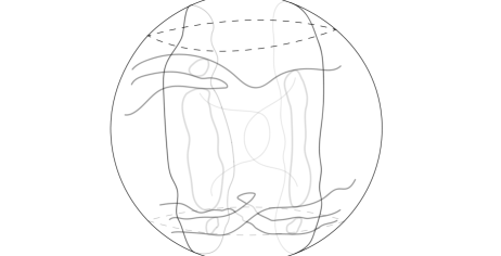
Figure 7. $\tilde{M}_{(J)}$ meeting with disks.

Suppose that $\mathbf{g}$ is the rank of $\Gamma$. We recall from Section 7 of [16]. Now $\Sigma_{+}$ denote the surface

$$(({\mathbb{S}}_{+}\cup\partial{\mathbb{S}}_{+})\setminus\Lambda_{\Gamma,{\mathbb{S}}_{+}})/\Gamma,$$

where ${\mathsf{S}}$ is a dense subset of $\Sigma_{+}$ with $\chi({\mathsf{S}})=1-\mathbf{g}$. Also, $\Sigma_{+}=({\mathbb{S}}_{+}\cup\bigcup_{i\in{\mathcal{I}}}a_{i})/\Gamma$. We add to $({\mathbb{S}}_{+}\cup\partial{\mathbb{S}}_{+})\setminus\Lambda_{\Gamma,{\mathbb{S}}_{+}}$ the set of ideal parabolic fixed points $a_{i},i\in\mathcal{I}^{\prime}\setminus\mathcal{I}$. The topology is given by a basis consisting of horodisks with fixed points added or the open disks in $({\mathbb{S}}_{+}\cup\partial{\mathbb{S}}_{+})\setminus\Lambda_{\Gamma,{\mathbb{S}}_{+}}$. We obtain a new surface $\hat{\Sigma}_{+}:={\mathbb{S}}_{+}\cup\bigcup_{i\in{\mathcal{I}}^{\prime}}a_{i}/\Gamma$.

We choose a collection $\{\hat{d}_{j}|j=1,\dots,m_{0}\}$ of disjoint geodesics ending at one of the ideal vertices or the boundary arc of $\hat{\Sigma}_{+}$ so that the complement of their union is the union of mutually disjoint open regions, each of which is homeomorphic to one of the following:

• a hexagon where three alternate edges are arcs in $\partial\hat{\Sigma}_{+}$,

• a pentagon with one ideal vertex (collapsed from a boundary component) and two alternate edges in $\partial\hat{\Sigma}_{+}$,

• a quadrilateral with two ideal vertices (collapsed from two boundary components) and one edge in $\partial\hat{\Sigma}_{+}$, or

• a triangle with three ideal vertices.

We may choose a set $\hat{d}_{i_{j}}$, $j=1,\dots,2{\mathbf{g}}$, where the complement of their union is a connected cell. We relabel these to be $\hat{d}_{1},\dots,\hat{d}_{2{\mathbf{g}}}$.

The lifts of the geodesics are geodesics in ${\mathbb{S}}_{+}$ ending at points of $\bigcup_{i\in{\mathcal{I}}}a_{i}$.

Lemma 5.8.

We can choose the mutually disjoint collection ${\mathcal{D}}_{j}\subset\mathsf{E}$ of properly embedded open disks and a tubular neighborhood $T_{j}\subset{\rm Cl}({\mathcal{D}}_{j})$ of $\partial{\mathcal{D}}_{j}$ for each $j$, $j=1,\dots,2{\mathbf{g}}$, that form a matching set $\{T_{j}|j=1,\dots,2{\mathbf{g}}\}$ for a collection $\mathcal{S}_{0}$ of generators of $\Gamma$. Finally, $\partial\mathcal{D}_{j}=d_{j}\cup\mathcal{A}(d_{j})\cup\bigcup_{x\in\partial d_{j}}{\rm Cl}(\zeta_{x})$ for a lift $d_{j}$ of $\hat{d}_{j}$.

Proof.

We choose lifts $d_{1},\dots,d_{2{\mathbf{g}}}$ of $\hat{d}_{1},\dots,\hat{d}_{\mathbf{g}}$ bounding a connected fundamental domain in ${\rm Cl}({\mathbb{S}}_{+})$. Since a component $L$ of

$${\mathbb{S}}_{+}\setminus\bigcup_{g\in\Gamma}\bigcup_{i=1}^{2{\mathbf{g}}}g(d_{j})$$

is the fundamental domain of the $\Gamma$-action on ${\mathbb{S}}_{+}$, we obtain $\gamma_{1},\dots,\gamma_{\mathbf{g}}$ generating $\Gamma$ forming a matching collection $\mathcal{S}_{0}$ by adding $\gamma_{1}^{-1},\dots,\gamma_{\mathbf{g}}^{-1}$. Label $\gamma_{j}^{-1}=\gamma_{{\mathbf{g}}+j}$ for $j=1,\dots,{\mathbf{g}}$. Hence, we may assume that $\gamma_{j}(d_{j})=d_{{\mathbf{g}}+j}$ for $j=1,\dots,2\mathbf{g},\hbox{ mod }2{\mathbf{g}}$ and $\{d_{1},\dots,d_{2{\mathbf{g}}}\}$ is a matching set for $\mathcal{S}_{0}$.

Let $p_{1},\dots,p_{m_{1}}$ denote the set of parabolic fixed points on any of $d_{j}$. By choosing the parabolic regions $R_{p_{1}},\dots,R_{p_{m_{1}}}$ sufficiently far away, we may assume that these are mutually disjoint. (See Section 3.3. Temporarily, we are not using the terminology of Section 5.1.1. )

We remove the interior of $R_{p_{j}},j=1,\dots,m_{1}$ from $\mathsf{E}$. Let $S_{p_{j}}$ denote the ruled surface boundary in $\mathsf{E}$ of $R_{p_{j}}$ where $\mathbf{g}_{j}^{t},t\in{\mathbb{R}}$ acts on. $R_{p_{j}}$ meets ${\mathbb{S}}_{+}$ in a closed horodisk ${\mathscr{H}}_{p_{j}}$. Then we define

(5.5) $$\tilde{\Sigma}^{\ast}:=\left(\tilde{\Sigma}\cup\bigcup_{j=1}^{m_{1}}S_{p_{j}}\right)\setminus\bigcup_{j=1}^{m_{1}}{\mathscr{H}}^{o}_{p_{j}}\setminus\bigcup_{j=1}^{m_{1}}{\mathscr{H}}^{o}_{p_{j},-}.$$

We assume that $d_{j}$ to be disjoint from ${\mathscr{H}}_{p_{k}}$ if $p_{k}$ is not an endpoint of $d_{j}$ by taking the cusp neighborhood sufficiently small.

• For each geodesic segment $d_{j}$ passing ${\mathscr{H}}_{p_{k}}$ for some $k$, we let $d^{\prime}_{j}:=d_{j}\cap\tilde{\Sigma}^{\ast}$. For each point of $x\in\partial d^{\prime}_{j}\cap{\mathbb{S}}_{+}$, we obtain a line $L_{x}$ in the ruled surface $S_{p_{j}}$. (See Appendix A.) We denote it by $\zeta_{x}$.

• For the endpoint of $d^{\prime}_{j}$ in $\partial{\mathbb{S}}_{+}$, i.e., in $\bigcup_{i\in\mathcal{I}}a_{i}$, we already defined $\zeta_{x}$ in Definition 3.3.

We define

$$\tilde{d}_{j}=d^{\prime}_{j}\cup\mathcal{A}(d^{\prime}_{j})\cup\bigcup_{x\in\partial d^{\prime}_{j}}{\rm Cl}(\zeta_{x}).$$

Then $\tilde{d}_{j}\cap\tilde{d}_{k}=\emptyset$ for $j\neq k$, $j,k=1,\dots,2{\mathbf{g}}$ since $\{d^{\prime}_{j}|j=1,\dots,2{\mathbf{g}}\}$ is a mutually disjoint collection of simple closed curves. Since $d_{j}\cap{\mathscr{H}}_{p_{k}}$ is a geodesic ending in $p_{k}$ or is empty for all $j,k$ by our choice, $d_{j}\cap\partial_{h}{\mathscr{H}}_{p_{k}}$ is the unique point or is empty. Also,

$$d_{j}\cap\partial_{h}{\mathscr{H}}_{p_{k}},j=1,\dots,2{\mathbf{g}},$$

are distinct for a fixed $k$ as $d_{j}$ are mutually disjoint. Thus, $\{{\rm Cl}(\zeta_{x}),x\in\partial d^{\prime}_{j}\}$ is a mutually disjoint collection.

Furthermore, $\tilde{d}_{1},\dots,\tilde{d}_{2{\mathbf{g}}}$ form a matching set for $\mathcal{S}_{0}$.

For each $x\in\partial d^{\prime}_{j}$, $j=1,\dots,{\mathbf{g}}$, we take

• for $x\in\partial{\mathbb{S}}_{+}$, a disk $Z_{x}$ of the form

  $$\bigcup_{y\in b}{\rm Cl}(\zeta_{y})\subset A_{k}=\bigcup_{y\in a_{k}}{\rm Cl}(\zeta_{y})$$

  where $b$ is a small open interval in $a_{k}$ and $x\in a_{k}\cap\partial d^{\prime}_{j}$, and

• for $x\in\partial{\mathscr{H}}_{p_{j}}$, a ruled tubular open neighborhood $Z_{x}$ of ${\rm Cl}(\zeta_{x})$ in the ruled surface ${\rm Cl}(S_{p_{j}})$.

Here, each $Z_{x}$, $x\in\partial d^{\prime}_{j}$, $j=1,\dots,\mathbf{g}$, is chosen sufficiently thin so that under elements of $\mathcal{S}_{0}$, the collection of $Z_{x}$ and their images is a collection of mutually disjoint sets. We take a union of all of these disks with

$$({\mathbb{S}}_{+}\cup{\mathbb{S}}_{-})\setminus\bigcup_{j=1}^{m}{{\mathscr{H}}}_{p_{j}}\setminus\bigcup_{j=1}^{m}{{\mathscr{H}}}_{p_{j},-}$$

to $\mathsf{E}\setminus\bigcup_{j=1}^{2{\mathbf{g}}}R_{p_{j}}$ to obtain a $3$-manifold with boundary. Then we can apply Theorem 5.3 for the simple closed curve $\tilde{d}_{j}$ to obtain open disks $\mathcal{D}^{\prime}_{j}$ so that $\tilde{d}_{j}=\partial\mathcal{D}^{\prime}_{j}$ for each $j=1,\dots,{\mathbf{g}}$. These are chosen to be mutually disjoint by the same theorem.

Then we obtain $\mathcal{D}^{\prime}_{j+{\mathbf{g}}}$ as the image $\gamma_{j}(\mathcal{D}^{\prime}_{j})$ for $\gamma_{j}\in\mathcal{S}_{0}$. Since the boundary components of $\mathcal{D^{\prime}}_{j}$, $j=1,\dots,2{\mathbf{g}}$, are mutually disjoint, using Theorem 5.3 again, we may do disk exchanges to obtain mutually disjoint disks $\mathcal{D}^{\prime\prime}_{j}$, $j=1,\dots,2{\mathbf{g}}$.

Let $p_{k}$ be a parabolic fixed point where $d_{j}$ ends. Now for each $\zeta_{x},x\in\partial d^{\prime}_{j}$, is in the boundary of a leaf of the foliation $\mathcal{D}_{f,r}$ in $R_{p_{k}}$ obtained by Theorem 3.14. For each such $p_{k}$ and $d_{j}$, we add the disk to $\mathcal{D}^{\prime}_{j}$ by joining them at each $\zeta_{x},x\in\partial d^{\prime}_{j}$. We call the results $\mathcal{D}_{j}$, $j=1,\dots,2{\mathbf{g}}$. These are mutually disjoint.

Now,

$${\rm Cl}(\mathcal{D}_{j})\cap{\rm Cl}(R_{p_{k}})\cap{\mathbb{S}}_{+}={\mathscr{H}}_{p_{k}}\cap d_{j}={\mathscr{H}}_{p_{k}}\cap\tilde{d}_{j}.$$

Hence, by adding these arcs back, we obtain

$$\partial\mathcal{D}_{j}=d_{j}\cup\mathcal{A}(d_{j})\cup\bigcup_{x\in\partial d_{j}}{\rm Cl}(\zeta_{x}).$$

Since we do not change the sufficiently thin tubular neighborhoods of $\partial\mathcal{D}_{j}$ under the above disk exchanges, there exists a matching collection of tubular neighborhoods $\{T_{j}|j=1,\dots,2{\mathbf{g}}\}$ of $\{\partial\mathcal{D}_{j}|j=1,\dots,2{\mathbf{g}}\}$ under $\mathcal{S}_{0}$.

∎

Here, of course, the disk collection is not yet a matching set under $\mathcal{S}_{0}$. By Lemma 5.8, the collection $\{{\rm Cl}({\mathcal{D}}_{j})\}$ are mutually disjoint in ${\rm Cl}(\mathsf{E})$. The collection ${\mathcal{D}}_{j}$, $j=1,2,\dots,2{\mathbf{g}}$, bound a region $\mathbf{F}$ closed in $\mathsf{E}$ with a compact closure in ${\rm Cl}(\mathsf{E})$, a finite-sided polytope in the topological sense.

Now we consider $K_{0}$ to be the set

$$\bigcup_{j=1}^{2{\mathbf{g}}}({\mathcal{D}}_{j}\setminus T_{j}^{o})\cup\bigcup_{1\leq j<k\leq 2{\mathbf{g}}}({\mathcal{D}}_{j}\cap{\mathcal{D}}_{k}).$$

By Proposition 5.1, we choose $M_{(J)}$ in our exhaustion sequence of $M$ so that

(5.6) $$\tilde{M}_{(J)}\supset N_{{\mathbf{d}},\epsilon}\left(K_{0}\right)$$

for an $\epsilon$-neighborhood, $\epsilon>0$.

5.2.4. Outside tameness

The following is enough to prove tameness.

Proposition 5.9 (Outside Tameness).

Let $M$ denote a Margulis space-time $\mathsf{E}/\Gamma$ where $\Gamma$ is an isometry group with $\mathcal{L}(\Gamma)\subset{\mathsf{SO}}(2,1)^{o}$. Let $\mathbf{F}$ be the domain bounded by $\bigcup_{i=1}^{2{\mathbf{g}}}{\mathcal{D}}_{i}$. Suppose that $M_{(J)}$ satisfies (5.6). Then $\mathbf{F}\setminus\tilde{M}_{(J)}$ is a fundamental domain of $M\setminus M_{(J)}$, and $M$ is tame. Furthermore, $\bigsqcup_{i=1}^{2{\mathbf{g}}}{\mathcal{D}}_{i}\setminus\tilde{M}_{(J)}$ embeds to a union of mutually disjoint properly embedded surfaces in $M$.

Proof.

By Corollary 5.7, $\mathbf{F}\setminus\tilde{M}_{(J)}^{o}$ is a tame $3$-manifold. Let $X$ denote $\mathbf{F}\setminus\tilde{M}_{(J)}^{o}$, a tame $3$-manifold bounded by a union of finitely many compact surfaces.

$$M_{(J+1)}\setminus M_{(J)}^{o}\subset M_{(J+2)}\setminus M_{(J)}^{o}\subset\cdots$$

is an exhausting sequence of compact submanifolds in $M\setminus M_{(J)}^{o}$. Since ${\mathcal{D}}_{i}\setminus\tilde{M}_{(J)}^{o}\subset T_{i}$,

$$\{{\mathcal{D}}_{i}\setminus\tilde{M}_{(J)}^{o}|i=1,\dots,2{\mathbf{g}}\}\subset{\rm bd}\mathbf{F}\cap\mathsf{E}$$

is a matching collection under $\mathcal{S}_{0}$ by Lemma 5.8. Also, $\mathbf{F}\cap(\tilde{M}_{(J+n)}\setminus\tilde{M}_{(J)}^{o})$ for each $n$ is a compact topological polytope by Corollary 5.7. By Proposition 2.6, $X$ is the fundamental domain of $\mathsf{E}\setminus\tilde{M}_{(J)}^{o}$. Hence, $M\setminus M_{(J)}^{o}$ is tame.

The tameness of $M$ follows since $M\setminus M_{(J)}^{o}$ and $M_{(J)}$ are tame. The last statement follows since $\bigsqcup_{i=1}^{2{\mathbf{g}}}{\mathcal{D}}_{i}\setminus\tilde{M}_{(J)}^{o}$ is the boundary of a fundamental domain in $\mathsf{E}\setminus\tilde{M}_{(J)}^{o}$. ∎

5.2.5. Considering the whole disks ${\mathcal{D}}_{i}\cap\tilde{M}_{(J)}$

We consider bounded components of ${\mathcal{D}}_{i}\setminus\tilde{M}_{(J)}^{o}$ for $i=1,\dots,2{\mathbf{g}}$. By Proposition 5.9, the union of these planar surfaces embeds to the union of disjoint ones in $M$. We take the mutually disjoint thin tubular neighborhoods of the images of compact planar components of ${\mathcal{D}}_{i}\setminus\tilde{M}_{(J)}^{o}$ and take the inverse image to $\mathsf{E}$. We add these to $\tilde{M}_{(J)}$. Let us call the result $\tilde{M}_{(J)}\subset\tilde{M}$ again. Since $\Gamma$ acts on $\tilde{M}_{(J)}$, we obtain a compact submanifold $M_{(J)}$ in $M$.

Thus, by Theorem 5.3 applied to $M_{(J)}$, each component of ${\mathcal{D}}_{i}\cap\partial\tilde{M}_{(J)}$ bounds a disk mapping to a mutually disjoint collection of embedded disks in $M_{(J)}$. We modify $\mathcal{D}_{i}$ by replacing each component of ${\mathcal{D}}_{i}\cap\tilde{M}_{(J)}$ with lifts of these disks. (See [30] and [32] for some details.)

The results are still embedded in $\tilde{M}$ since we modify only inside $\tilde{M}_{(J)}$ where the disks are also disjoint.

Hence, we conclude

$$\gamma_{j}({\mathcal{D}}_{j})={\mathcal{D}}_{j+{\mathbf{g}}} \hbox{ for }\gamma_{j}\in\mathcal{S},\hbox{ and }$$

(5.7) $$\gamma_{j}({\mathcal{D}}_{l})\cap{\mathcal{D}}_{m}=\emptyset \hbox{ for }(j,l,m)\neq(j,j,j+{\mathbf{g}})\mod 2{\mathbf{g}}.$$

We summarize

Proposition 5.10.

Let $M$ denote a Margulis space-time $\mathsf{E}/\Gamma$ where $\Gamma$ is an isometry group with $\mathcal{L}(\Gamma)\subset{\mathsf{SO}}(2,1)^{o}$. Then there exists a fundamental domain $\mathcal{R}$ closed in $\mathsf{E}$ bounded by finitely many crooked-circle disks $\mathcal{D}_{j}$, $j=1,\dots,2{\mathbf{g}}$. Moreover, ${\rm Cl}(\mathcal{R})\cap(\mathsf{E}\cup\tilde{\Sigma})$ is the fundamental domain of a manifold $(\mathsf{E}\cup\tilde{\Sigma})/\Gamma$ with boundary $\Sigma$. Here, $\mathcal{R}^{o}$ and ${\rm Cl}(\mathcal{R})$ are $3$-cells, and $\mathsf{E}/\Gamma$ is homeomorphic to the interior of a handlebody of genus $\mathbf{g}$.

Proof.

Let $\mathcal{R}$ be the region in $\mathsf{E}$ with boundary equal to $\bigcup_{j=1}^{2{\mathbf{g}}}\mathcal{D}_{j}$. Since $\mathcal{D}_{j}$ is a properly embedded separating disk in a cell, repeated applications of Lemma 1.12 of [36] imply that $\mathcal{R}^{o}$ is a cell. Since ${\rm Cl}(\mathcal{R})$ is a polyhedral manifold whose interior is a $3$-cell, it is a $3$-cell.

Since by (5.2.5),

$$\{\mathcal{D}_{j}|j=1,\dots,2{\mathbf{g}}\}$$

is a matched set under $\mathcal{S}_{0}$, $\mathcal{R}$ is the fundamental domain by Proposition 2.6. The quotient space is homeomorphic to the interior of a handlebody since we can find a homeomorphism of $\mathcal{R}$ to the standard $3$-ball where $\mathcal{D}_{j}$, $i=1,\dots,2{\mathbf{g}}$, correspond to disjoint open disks with piecewise smooth boundary.

Also,

$$\{{\rm Cl}(\mathcal{D}_{j})\cap(\mathsf{E}\cup\tilde{\Sigma})|j=1,\dots,2{\mathbf{g}}\}$$

is a matched set under $\mathcal{S}_{0}$. Also, every point in $\tilde{N}:=\mathsf{E}\cup\tilde{\Sigma}$ is equivalent to a point of $\mathcal{R}^{\prime}:={\rm Cl}(\mathcal{R})\cap\tilde{N}$ by the action of $\Gamma$. Hence, $\mathcal{R}^{\prime}$ is a fundamental domain giving us the properness of the action of $\Gamma$ on $\tilde{N}:=\mathsf{E}\cup\tilde{\Sigma}$. Thus, $\tilde{N}/\Gamma$ is a manifold with boundary $\Sigma$.

∎

This proves the first part of Theorem 1.1. The remaining part of Theorem 1.1 will be completed in Section 5.4.

5.3. Parabolic regions and the intersection properties

We will now choose the parabolic regions so that their images under the deck transformation groups are mutually disjoint. We will need this in Proposition 5.13.

The basic idea used is that disks are separating $\mathsf{E}$ into two components. We choose the parabolic regions for each parabolic point in the closure of the fundamental domain so that they meet the fundamental domain $\mathcal{R}$ is in a nice manner. Using this, we can show that each image of a parabolic region meets an image of the fundamental domain in finitely many manners. This will essentially give us the needed intersection properties.

The above fundamental domain $\mathcal{R}$ is bounded by a union of disks $\mathcal{D}_{i},i=1,\dots,2{\mathbf{g}}$, in the boundary of $\mathcal{R}$. We call $\mathcal{D}_{i}$ the facial disks of $\mathcal{R}$. By construction, the closure of $\mathcal{D}_{i}$ is disjoint from $\Lambda_{\Gamma,{\mathbb{S}}_{+}}\subset\partial{\mathbb{S}}_{+}$ except for parabolic points. The set of parabolic points meeting at least one ${\rm Cl}(\mathcal{D}_{i})$ is a finite set $\{p_{1},\dots,p_{m_{1}}\}$. (Possibly two or more of $p_{i}$s may be in the same orbit of $\Gamma$.)

We use the notations of Section 5.1.1. For each $p_{i}$, $i=1,\dots,m_{1}$, we have a parabolic region of the form $\gamma(\mathcal{P}_{j})$ for some $j$, $j=1,\dots,m_{0}$, and $\gamma\in\Gamma$ whose closure contains $p_{i}$. For each $i$, we denote by $\mathcal{P}_{i}$ this region $\gamma(\mathcal{P}_{j})$. We denote by $\eta_{i}$ the parabolic element fixing $p_{i}$, following the boundary orientation if we remove $E$, and hence $\eta_{i}=\gamma\eta_{j}\gamma^{-1}$ for some $j=1,\dots,m_{0}$.

Now, we choose $\mathcal{P}_{j}$, $j=1,\dots,m_{0}$, so that ${\rm Cl}(\mathcal{P}_{i})\cap{\mathbb{S}}_{+}$ for each $i$ equals a component of the inverse image of $E$. These $R_{j}$, $j=1,\dots,m_{0}$, form a mutually disjoint collection of closed cusp neighborhoods of ${\mathsf{S}}$ as given in Section 2.2. ${\rm Cl}(\mathcal{P}_{i})\cap{\mathbb{S}}_{+}$ for each $i$ equals a component of the inverse image of $E$. Also, by our construction in Theorem 3.13, we have ${\rm Cl}(\mathcal{P}_{i})\cap{\mathbb{S}}_{-}=\mathcal{A}({\rm Cl}(\mathcal{P}_{i})\cap{\mathbb{S}}_{+}).$

Definition 5.2.

Let $p_{i}$ and $\mathcal{P}_{i}$ be as above for $i\in{\mathcal{I}}^{\prime}\setminus{\mathcal{I}}$, and let $\eta_{i}$ be the parabolic primitive element fixing $p_{i}$. Let $D_{f_{i},r_{i},t}$ denote the canonically defined properly embedded disks by Theorem 3.14. We say that an image $\gamma(\mathcal{R})$, $\gamma\in\Gamma$, of the fundamental domain $\mathcal{R}$ bounded by crooked-circle disks meets nicely with $\eta(\mathcal{P}_{i})$, $\eta\in\Gamma$, if

(5.8) $$\eta(\mathcal{P}_{i})\cap\gamma(\mathcal{R})=\bigcup_{t\in[t_{1},t_{2}]}D_{f_{i},r_{i},t}\hbox{ for some }t_{1},t_{2}\in{\mathbb{R}},t_{1}<t_{2}$$

and

(5.9) $${\rm Cl}(\zeta_{\eta(p_{i})}) \subset{\rm Cl}(\gamma(\mathcal{R})),\hbox{ and }$$

(5.10) $$\eta(\mathcal{P}_{i}) \subset\left(\bigcup_{k\in{\mathbb{Z}}}\gamma\eta_{i}^{k}\left(\bigcup_{j=1}^{k_{0}}\kappa_{j}(\mathcal{R})\right)\right)^{o}$$

for a finite collection of $\{\kappa_{j}\in\Gamma\}$ where ${\rm Cl}(\zeta_{\eta(p_{i})})\subset{\rm Cl}(\gamma(\kappa_{j}(\mathcal{R})))$.

Of course, by the definition $\gamma\circ\eta_{i}^{k}\circ\kappa_{j}(\mathcal{R})$, $k\in{\mathbb{Z}}$, meets with $\eta(\mathcal{P}_{j})$ nicely as well.

Lemma 5.11.

Let $\Gamma$ satisfy Criterion 1.1. Let $\mathcal{R}$ be the fundamental domain of $\mathsf{E}/\Gamma$ bounded by crooked-cricle disks as constructed by Proposition 5.10. Let $q$ be a parabolic fixed point in ${\rm Cl}(\mathcal{R})$. Then $q=p_{i}$ for some $i$, $i=1,\dots,m_{1}$. Moreover, the following hold:

• ${\rm Cl}(\zeta_{p_{i}})\subset{\rm Cl}(\mathcal{R})$,

• ${\rm Cl}(\zeta_{p_{i}})$ is a subset of the closures of exactly two facial disks $\mathcal{D}_{l}$ and $\mathcal{D}_{m}$ among the facial disks of $\mathcal{R}$, and

• the corresponding parabolic region $\mathcal{P}_{i}$ meets nicely with $\mathcal{R}$ provided we choose $\mathcal{P}_{i}$, $i=1,\dots,m_{0}$, sufficiently far away.

Proof.

Since $q\in{\rm Cl}(\mathcal{R})$, $q=p_{i}$ by the construction in Lemma 5.8 of $\partial\mathcal{D}_{j}$, $j=1,\dots,2{\mathbf{g}}$. Since the closure of $\mathcal{D}_{j}$ is compact, either $\mathcal{D}_{j}$ contains $\zeta_{p_{i}}$ in its boundary, or there is an $\epsilon$-${\mathbf{d}}$-neighborhood of ${\rm Cl}(\zeta_{p_{i}})$ disjoint from it for some $\epsilon>0$. We can choose the boundary ruled surface of $\mathcal{P}_{i}$ sufficiently far so that (5.8) holds and hence only facial disks of $\mathcal{R}$ that meet $\mathcal{P}_{i}$ are the two facial disks whose closures contain $\zeta_{p_{i}}$. (See Definition 3.5.) Let us call these $\mathcal{D}_{j}$ and $\mathcal{D}_{k}$.

Now, $\partial\mathcal{P}_{i}\cap\mathsf{E}=S_{i}$ is an open disk separating $\mathcal{P}_{i}$ from $\mathsf{E}\setminus{\rm Cl}(\mathcal{P}_{i})$. $\partial\mathcal{P}_{i}\cap\mathcal{R}$ has the boundary formed by two lines respectively in $\mathcal{D}_{j}$ and $\mathcal{D}_{k}$. We take finitely many images $\kappa_{l}({\mathcal{R}}),l=1,\dots,k_{0}$ of $\mathcal{R}$ with $\kappa_{1}={\rm I}$ so that $\kappa_{l}(\mathcal{R})\cap\kappa_{l+1}(\mathcal{R})$ is a copy of $\mathcal{D}_{i_{0}}$ for some $i_{0}$ whose closure contains $\zeta_{p_{i}}$. Since the collection $\{\gamma(\mathcal{R}),\gamma\in\Gamma\}$ tessellates $\mathsf{E}$, we can choose enough of $\kappa_{j}$ so that $\kappa_{k_{0}+1}(\mathcal{R})=\eta_{i}^{\pm 1}(\kappa_{1}(\mathcal{R}))$ for either $+$ or $-$ sign.

Except for the closures of facial disks of $\{\kappa_{j}(\mathcal{R})|j=1,\dots,k_{0}\}$ containing ${\rm Cl}(\zeta_{p_{i}})$, the closures of other facial disks contained in the boundary of

$$\{\kappa_{j}(\mathcal{R})|j=1,\dots,k_{0}\}$$

are disjoint from ${\rm Cl}(\zeta_{p_{i}})$. Let $\hat{K}$ denote the union of the closures of these images of facial disks of $\{\kappa_{j}(\mathcal{R})|j=1,\dots,k_{0}\}$ disjoint from ${\rm Cl}(\zeta_{p_{i}})$. Since these are separating disks in $\mathcal{H}$, we may choose $\mathcal{P}_{i}$ sufficiently far so that ${\rm Cl}(\mathcal{P}_{i})\cap\hat{K}=\emptyset$.

Since ${\rm Cl}(\mathcal{P}_{i})$ is $\eta_{i}$-invariant, ${\rm Cl}(\mathcal{P}_{i})$ is disjoint from $\bigcup_{m\in{\mathbb{Z}}}\eta_{i}^{m}(\hat{K})$. Now, $\bigcup_{m\in{\mathbb{Z}}}\eta_{i}^{m}(\hat{K})$ is a separating set in $\mathsf{E}$. A component of $\mathsf{E}\setminus\bigcup_{m\in{\mathbb{Z}}}\eta_{i}^{m}(\hat{K})$ equals

$$\left(\bigcup_{k\in{\mathbb{Z}}}\eta_{i}^{k}\left(\bigcup_{j=1}^{k_{0}}\kappa_{j}(\mathcal{R})\right)\right)^{o}.$$

Since $\mathcal{P}_{i}$ is a connected set, we obtain

(5.11) $$\mathcal{P}_{i}\subset\left(\bigcup_{k\in{\mathbb{Z}}}\eta_{i}^{k}\left(\bigcup_{j=1}^{k_{0}}\kappa_{j}(\mathcal{R})\right)\right)^{o}.$$

∎

Notice that (5.11) gives us the conditions of Definition 5.2.

Proposition 5.12.

Let $\mathcal{P}_{i}$ be a parabolic region for the parabolic fixed point $p_{i}$, $i=1,\dots,m_{0}$, as we chose at the beginning of Section 5.3. We can always choose $\mathcal{P}_{i},i=1,\dots,m_{0}$, so that for every pair $\eta,\gamma\in\Gamma$, so that exclusively one of the following holds :

• $\eta(p_{i})\not\in\gamma({\rm Cl}(\mathcal{R}))$, or else

• $\gamma(\mathcal{R})$ meets $\eta(\mathcal{P}_{i})$ nicely, and $\gamma(\mathcal{P}_{j})=\eta(\mathcal{P}_{i})$ for some $j=1,\dots,m_{1}$.

Proof.

We may assume $\gamma={\rm I}$ since we can change $\eta$ to $\gamma^{-1}\eta$. Then the result follows by Lemma 5.11. ∎

We choose $\mathcal{P}_{j}$ far away for $j=1,\dots,m_{0}$ so that the conclusions of Proposition 5.12 are satisfied.

Let $P=\bigcup_{\gamma\in\Gamma}\bigcup_{i=1,\dots,m_{0}}\gamma(\mathcal{P}_{i})$, and let $\mathcal{P}_{\mathcal{R}}:=(\mathcal{P}_{1}\cup\cdots\cup\mathcal{P}_{m_{1}})\cap\mathcal{R}$.

Proposition 5.13.

We can choose the sufficiently far away parabolic regions

$$\mathcal{P}_{1},\dots,\mathcal{P}_{m_{0}}$$

meeting $\mathcal{R}$ nicely so that they are disjoint in $\mathsf{E}$. Then the following hold :

• The following are equivalent:

  1. $\gamma(\mathcal{P}_{i})$ meets $\mathcal{R}$ nicely.

  2. $\gamma(\mathcal{P}_{i})=\mathcal{P}_{j}$ for some $j$, $j=1,\dots,m_{1}$.

  3. $\gamma(\mathcal{P}_{i})\cap\mathcal{R}\neq\emptyset$.

• $\mathcal{R}$ meets only $\mathcal{P}_{1},\dots,\mathcal{P}_{m_{1}}$ among all images $\gamma(\mathcal{P}_{r})$ for $\gamma\in\Gamma,r=1,\dots,m_{0}$.

• Moreover, for every pair $\gamma,\eta\in\Gamma$,

  $$\gamma(\mathcal{P}_{j})\cap\eta(\mathcal{P}_{k})=\emptyset\hbox{ or }\gamma(\mathcal{P}_{j})=\eta(\mathcal{P}_{k}),\,j,k=1,\dots,m_{0}.$$

Proof.

We first choose $\mathcal{P}_{i},i=1,\dots,m_{0}$, sufficiently far so that $\mathcal{P}_{i}\cap\mathcal{P}_{j}\cap\mathcal{R}=\emptyset$ for $i\neq j$, $i,j=1,\dots,m_{1}$, and every $\mathcal{P}_{j}$, $j=1,\dots,m_{1}$, meets $\mathcal{R}$ nicely by Proposition 5.12.

Obviously (2) implies (1). For the first item, we show that (1) implies (2): Suppose $\gamma(\mathcal{P}_{j})$ meets $\mathcal{R}$ nicely. Then $\gamma(p_{j})$ is in ${\rm Cl}(\mathcal{R})$. Since $\gamma(p_{j})$ is a parabolic fixed point, it equals $p_{l}$ for some $l=1,\dots,m_{1}$. Only elements of $\Gamma$ fixing $p_{l}$ are of the form $\eta_{l}^{m}$ for some integer $m\in{\mathbb{Z}}$.

$$\gamma({\rm Cl}(\mathcal{P}_{j}))\cap{\mathbb{S}}_{+}=\gamma({\mathscr{H}}_{k})\cup\gamma(\partial_{h}{{\mathscr{H}}_{k}})$$

for a horodisk ${\mathscr{H}}_{k}$. Now, $\gamma({\mathscr{H}}_{k})={\mathscr{H}}_{l}$. Hence, the parabolic group acting on $\gamma(\mathcal{P}_{j})$ is the same one acting on $\mathcal{P}_{l}$. By our choice of $\mathcal{P}_{j}$ in Section 5.3 from choosing orbit representatives of parabolic fixed points, we obtain

$$\gamma(\mathcal{P}_{j})=\mathcal{P}_{l}\hbox{ for some }l=1,\dots,m_{1}.$$

Clearly, (2) implies (3) by Lemma 5.11.

Now we show that (3) implies (2): Suppose that $\gamma(\mathcal{P}_{j})\cap\mathcal{R}\neq\emptyset$. Now, $\gamma(p_{j})\in\eta({\rm Cl}(\mathcal{R}))$ for some $\eta\in\Gamma$, and $\gamma(\mathcal{P}_{j})$ meets $\eta(\mathcal{R})$ nicely and $\gamma(\mathcal{P}_{j})=\eta(\mathcal{P}_{k})$ for some $k$ by Proposition 5.12. Moreover,

(5.12) $$\eta(\mathcal{P}_{k})\subset\left(\bigcup_{l\in{\mathbb{Z}}}\eta\eta_{k}^{l}\left(\bigcup_{r=1}^{k_{0}}\kappa_{r}(\mathcal{R})\right)\right)^{o}$$

by Proposition 5.12. Hence, $\gamma(\mathcal{P}_{j})$ meets with only the images of $\mathcal{R}$ of the form $\eta\eta_{k}^{l}\kappa_{j}(\mathcal{R})$. If

$$\eta\eta_{k}^{l}\left(\kappa_{j}(\mathcal{R})\right)=\mathcal{R}\hbox{ for some }k,l,j,$$

then $\gamma(\mathcal{P}_{j})$ meets $\mathcal{R}$ nicely since we can check Definition 5.2. If $\eta\eta_{k}^{l}\left(\kappa_{j}(\mathcal{R})\right)\neq\mathcal{R}$ for all $k,l,j$, then $\gamma(\mathcal{P}_{j})$ does not meet $\mathcal{R}$ by (5.12). (2) implies (1) by Lemma 5.11. We proved the first item.

The second item follows from it.

Suppose that two respective images $P^{\prime}_{i}$ and $P^{\prime}_{j}$ of some $\mathcal{P}_{k}$ and $\mathcal{P}_{l}$ for $k,l=1,\dots,m_{0}$ meets in a nonempty set. Hence, they meet in $\gamma(\mathcal{R})$ for some $\gamma\in\Gamma$. Thus,

$$\gamma^{-1}(P^{\prime}_{i})\cap\gamma^{-1}({P}^{\prime}_{j})\cap\mathcal{R}\neq\emptyset.$$

The first item implies that

$$\mathcal{P}_{j}=\gamma^{-1}(P^{\prime}_{i})\hbox{ and }\mathcal{P}_{l}=\gamma^{-1}({P}^{\prime}_{j})\hbox{ for some }l,m=1,\dots,m_{1}$$

However, $\mathcal{P}_{j}\cap\mathcal{P}_{l}\cap\mathcal{R}=\emptyset$ or $P^{\prime}_{i}=P^{\prime}_{j}$ by our construction of parabolic regions.

∎

5.4. Relative compactification

5.4.1. Proof of Theorem 1.1

Proposition 5.10 proves the first part of the theorem. First, we recall our bordifying surface as defined by (5.1):

$$\tilde{\Sigma}_{0}:={\mathbb{S}}_{+}\cup{\mathbb{S}}_{-}\cup\bigcup_{i\in{\mathcal{I}}}(A_{i}\cup a_{i}\cup\mathcal{A}(a_{i})).$$

$\Sigma:=\tilde{\Sigma}_{0}/\Gamma$ and $N:=(\mathsf{E}\cup\tilde{\Sigma})/\Gamma$, which is a manifold by Proposition 5.10.

By Proposition 5.13, we define $P$ to be a union of mutually disjoint parabolic regions of the form $\gamma(\mathcal{P}_{i})$ for $\gamma\in\Gamma$, $i=1,\dots,m_{0}$. Since the boundary of their union in ${\mathbb{S}}$ is the union of mutually disjoint closed horodisks, their closures in $\mathcal{H}={\rm Cl}(\mathsf{E})$ are mutually disjoint. Now, we take the closure ${\rm Cl}(P)$ of $P$ and take the relative interior $P^{\prime}$ in the closed hemisphere $\mathcal{H}$. Let $\partial_{\mathsf{E}}P^{\prime}$ denote ${\rm bd}P^{\prime}\cap\mathsf{E}$. Then define $\tilde{N}^{\prime}:=(\mathsf{E}\cup\tilde{\Sigma})\setminus P^{\prime}$. $\Gamma$ acts properly discontinuously on $\tilde{N}^{\prime}$ since $\tilde{N}^{\prime}$ is a $\Gamma$-invariant proper subspace of $\tilde{N}$. We note that $\partial_{\mathsf{E}}P^{\prime}$ is transversal to ${\mathbb{S}}$. Thus, $N^{\prime}:=\tilde{N}^{\prime}/\Gamma$ is a manifold.

The manifold boundary $\partial N^{\prime}$ of $N^{\prime}$ is

$$((\tilde{\Sigma}\setminus P^{\prime})\cup\partial_{\mathsf{E}}P^{\prime})/\Gamma.$$

Define $P^{\prime\prime}=P^{\prime}/\Gamma$. Also, $(\partial_{\mathsf{E}}P^{\prime})/\Gamma$ is a union of a finite number of disjoint annuli. $\partial N^{\prime}$ is homeomorphic to $(\Sigma\setminus P^{\prime\prime})\cup(\partial_{\mathsf{E}}P^{\prime})/\Gamma$.

Recall that the union of facial disks $\mathcal{D}_{i}$, $i=1,\dots,2{\mathbf{g}}$, bounds the fundamental domain $\mathcal{R}$ in $\mathcal{H}$. Then

$$\bigcup_{i=1}^{2{\mathbf{g}}}{\rm Cl}(\mathcal{D}_{i})\cap((\mathsf{E}\cup\tilde{\Sigma})\setminus P^{\prime})$$

bounds a fundamental domain

$${\rm Cl}(\mathcal{R})\cap((\mathsf{E}\cup\tilde{\Sigma})\setminus P^{\prime}).$$

The boundary is homeomorphic to a $2$-sphere and, hence, the fundamental domain is homeomorphic to a compact $3$-cell. Since this fundamental domain is compact, $N^{\prime}$ is compact.

Since we pasted disjoint disks on a cell, $N^{\prime}$ is homotopy equivalent to a bouquet of circles. Now, $N^{\prime}$ has no fake-cell since $\tilde{N}^{\prime}$ is a subset of $\mathsf{E}$. It follows that $N^{\prime}$ is homeomorphic to a compact handlebody of genus $\mathsf{g}$ by Theorem 5.2 of [32].

Let $\hat{P}$ be the closure of $P^{\prime}$ in $\tilde{N}$. We realize that $N^{\prime}$ is a deformation retract of $N$ by collapsing $\hat{P}/\Gamma$, homeomorphic to a disjoint union of copies of $A^{2}\times[0,1)$, to its boundary in $N$ homeomorphic to a disjoint union of embedded images of $A^{2}$ for a compact annulus $A^{2}$ with boundary. This completes the proof of Theorem 1.1.

5.4.2. Proof of Corollary 1.2

If $\mathcal{L}(\Gamma)\subset{\mathsf{SO}}(2,1)^{o}$, we are done by Theorem 1.1.

Suppose not. We have an index-two subgroup $\Gamma^{\prime}$ of $\Gamma$ acting on ${\mathbb{S}}_{+}$ with $\mathcal{L}(\Gamma^{\prime})\subset{\mathsf{SO}}(2,1)^{o}$. Then $\Gamma^{\prime}$ acts on $(\mathsf{E}\cup\tilde{\Sigma})\setminus P^{\prime}$ where we construct $\tilde{\Sigma}$ and $P^{\prime}$ as above for $\Gamma^{\prime}$. There exists an element $\phi$ of $\Gamma-\Gamma^{\prime}$ so that $\phi({\mathbb{S}}_{+})={\mathbb{S}}_{-}$ and $\phi^{2}\in\Gamma^{\prime}$ and $\phi$ normalizes $\Gamma^{\prime}$. Since $\phi$ acts as an orientation-preserving map of ${\mathbb{S}}$, and

$$\mathcal{L}(\phi)\circ\mathcal{L}(\Gamma^{\prime})\circ\mathcal{L}(\phi)^{-1}=\mathcal{L}(\Gamma^{\prime}),$$

it follows that $\phi$ induces a diffeomorphism ${\mathbb{S}}_{+}/\Gamma^{\prime}$ with ${\mathbb{S}}_{-}/\Gamma^{\prime}$ preserving orientations. Since ${\mathbb{S}}_{-}$ is a Klein model also, we can define a limit set $\Lambda_{\Gamma^{\prime},{\mathbb{S}}_{-}}$. Hence, for the limit sets, we have

$$\phi(\Lambda_{\Gamma^{\prime},{\mathbb{S}}_{+}})=\Lambda_{\Gamma^{\prime},{\mathbb{S}}_{-}},\hbox{ and }\phi(\partial{\mathbb{S}}_{+}\setminus\Lambda_{\Gamma^{\prime},{\mathbb{S}}_{+}})=\partial{\mathbb{S}}_{-}\setminus\Lambda_{\Gamma^{\prime},{\mathbb{S}}_{-}}.$$

Since each element of $\mathcal{L}(\Gamma^{\prime})$ commutes with $\mathcal{A}$, we obtain

$$\mathcal{A}(\Lambda_{\Gamma^{\prime},{\mathbb{S}}_{+}})=\Lambda_{\Gamma^{\prime},{\mathbb{S}}_{-}}\hbox{ and }\mathcal{A}(\partial{\mathbb{S}}_{+}\setminus\Lambda_{\Gamma^{\prime},{\mathbb{S}}_{+}})=\partial{\mathbb{S}}_{-}\setminus\Lambda_{\Gamma^{\prime},{\mathbb{S}}_{-}}.$$

Let $\mathcal{I}$ denote the collection of open intervals of $\partial{\mathbb{S}}_{+}\setminus\Lambda_{\Gamma^{\prime},{\mathbb{S}}_{+}}$. We define $\tilde{\Sigma}$ for $\Gamma^{\prime}$ as in (5.1),

$${\mathbb{S}}_{+}\cup{\mathbb{S}}_{-}\cup\bigcup_{a\in\mathcal{I}}\left(a\cup\mathcal{A}(a)\cup\bigcup_{x\in a}\zeta_{x}\right).$$

Since $\phi$ is orientation-preserving, $\phi$ sends the disk $A_{a}=\bigcup_{x\in a}\zeta_{x}$, $a\in\mathcal{I}$, to $A_{\mathcal{A}(\phi(a))}$. Since $a\mapsto\mathcal{A}\phi(a)$ gives us an automorphism of $\mathcal{I}$, $\phi$ acts on $\tilde{\Sigma}$.

Given a component $P_{1}$ of $P^{\prime}$, there is a parabolic primitive element $\gamma_{1}$ acting on it. Then $\gamma_{2}:=\phi\circ\gamma_{1}\circ\phi^{-1}$ acts on $\phi(P_{1})$. Since $\gamma_{2}\in\Gamma^{\prime}$ also, $\gamma_{2}$ acts on a component $P_{2}$ of $P^{\prime}$. We denote $\gamma_{2}^{\ast}(P_{1})=P_{2}$ where we may not yet have $\gamma(P_{1})=P_{2}$.

Let $\widetilde{\mathcal{P}}$ denote the set of parabolic fixed points of $\partial{\mathbb{S}}_{+}$. Then let a finite $\hat{\mathcal{P}}$ denote the collection of the $\Gamma^{\prime}$-orbit classes of $\widetilde{\mathcal{P}}$. The above action of $\phi$ induces an automorphism of $\hat{\mathcal{P}}$.

Lemma 5.14.

There is no fixed point in $\hat{P}$ under this action of $\phi$ on $\hat{\mathcal{P}}$.

Proof.

Suppose not. Then using orbit equivalence under $\Gamma$, there exists an isometry $\psi\in\Gamma\setminus\Gamma^{\prime}$ so that $\mathcal{A}\circ\mathcal{L}(\psi)(q)=q$ for a parabolic fixed point $q$. $\mathcal{A}\circ\mathcal{L}(\psi)$ acts on ${\mathbb{S}}_{+}$ acting on a component ${\mathscr{H}}_{i}$ for some $i$. Since $\mathcal{A}\circ\mathcal{L}(\psi)$ acts as an orientation reversing isometry on ${\mathbb{S}}_{+}$, $\mathcal{A}\circ\mathcal{L}(\psi)$ acts on a complete geodesic $l_{q}$ ending at $q$. Since it must fix the point $\partial_{h}{\mathscr{H}}_{i}\cap l_{q}$, it fixes each point of $l_{q}$. Hence, $\mathcal{L}(\psi)$ acts as $-{\rm I}$ on a time-like vector subspace $P_{l_{q}}$ corresponding to $l_{q}$, and is the identity on a space-like vector subspace. Since $\psi$ cannot have a fixed point on $\mathsf{E}$, $\psi^{2}$ cannot be the identity on $\mathsf{E}$, and it is a Lorentzian translation on a space-like geodesic $l$ orthogonal to $P_{l_{q}}$, and $\psi^{2}\in\Gamma^{\prime}$ since $[\Gamma:\Gamma^{\prime}]=2$. However, $\Gamma^{\prime}$ does not have a translation element as it is an affine deformation of $\mathcal{L}(\Gamma^{\prime})$. ∎

Since there is no fixed point of the action, we divide the collection $\mathcal{\hat{P}}$ of components of $P^{\prime}$ into equivalence classes of orbits under $\Gamma^{\prime}$. This is a finite set $\hat{P}_{1},\dots,\hat{P}_{2m}$. Now $\phi$ acts on this set. We may assume that $\phi$ sends $\hat{P}_{i}$ to $\hat{P}_{m+i}$.

We replace each element of $\hat{P}_{m+i}$ with $\phi(P^{\prime\prime})$ for the corresponding element $P^{\prime\prime}$ of $\hat{P}_{i}$ for $i=1,\dots,m$. We obtain a new set $P^{\prime}$. Here, for the parabolic element $\gamma^{\prime\prime\prime}$ corresponding to $\phi(P^{\prime\prime})$, we have $\gamma^{\prime\prime\prime}=\phi\circ\gamma^{\prime\prime}\circ\phi^{-1}$ for a parabolic element $\gamma^{\prime\prime}$ acting on $P^{\prime\prime}$. Since $\gamma^{\prime\prime\prime}$ is in the unique one-parameter subgroup $\gamma^{\prime\prime\prime t},t\in{\mathbb{R}},$ of parabolic isometries, $\gamma^{\prime\prime\prime t},t\in{\mathbb{R}},$ acts on $\phi(P^{\prime\prime})$. Therefore, the boundary $\partial\phi(P^{\prime\prime})\cap\mathsf{E}$ is a parabolic ruled surface for $\gamma^{\prime\prime\prime}$ as defined by Definition 3.5.

Obviously, $\Gamma$ acts on $P^{\prime}$. Also, we may assume that elements of $P^{\prime}$ are mutually disjoint: we take a finite set of components of $P^{\prime}$ that meets the fundamental domain $\mathcal{R}$. We can make these disjoint by taking them sufficiently far away. Proposition 5.13 shows that these are mutually disjoint.

Therefore, $N^{\prime}:=((\mathsf{E}\cup\tilde{\Sigma})\setminus P^{\prime})/\Gamma$ is compact and is homeomorphic to a handlebody of genus $\mathsf{g}$ by Theorem 5.2 of [32] as in Section 5.4.1. Since $\phi$ does not act on any component of $P^{\prime}$, we can show that $N$ deformation retracts to $N^{\prime}$ as above.

Appendix A Parabolic ruled surfaces

We will be using the parabolic coordinate system obtained in Section 3.1. These constructions are canonical except for the ambiguity in the $x$-coordinates up to translations. (See Remark 3.1.)

A.1. Proper embedding of ruled surfaces

Only prerequisites are Sections 2 and 3.1. Our purpose is to prove Theorem 3.13 using Lemma A.1, Proposition A.2, and Lemma A.3.

Lemma A.1.

Assume as in Theorem 3.13. Every $g^{t}$-orbit in $\mathcal{H}_{\kappa_{1},\kappa_{2}}$ starts and ends at ${\zeta_{\left(\mkern-4.0mu\left(1,0,0,0\right)\mkern-4.0mu\right)}}$.

Proof.

Let $l$ be a segment so that ${\rm Cl}(l)\in\mathcal{H}_{s_{0},\kappa_{1},\kappa_{2}}$. An endpoint of $l_{\infty}$ must be $\left(\mkern-4.0mu\left(1,0,0,0\right)\mkern-4.0mu\right)\,\,$ since $g^{t_{i}}(q)\rightarrow\left(\mkern-4.0mu\left(1,0,0,0\right)\mkern-4.0mu\right)$ for each point $q\in l\cap P_{T}$. Since ${\rm Cl}(l)$ has a pair of antipodal points, the other endpoint of ${\rm Cl}(l_{\infty})$ is $\left(\mkern-4.0mu\left(-1,0,0,0\right)\mkern-4.0mu\right)$. We compute the intersection of an arbitrary image of $g^{t}(l)$ at the plane given by $x=0$

(A.1) $$\left(\mkern-4.0mu\left(0,-\frac{ct\left(\mu t^{3}+6ty_{0}\right)}{6a+3ct^{2}}+\frac{\mu t^{2}}{2}+y_{0},\mu t-\frac{c\left(\mu t^{3}+6ty_{0}\right)}{6a+3ct^{2}},1\right)\mkern-4.0mu\right)=\\ \left(\mkern-4.0mu\left(0,-\frac{\mu t^{2}+6y_{0}}{\frac{6a}{ct^{2}}+3}+\frac{\mu t^{2}}{2}+y_{0},\mu t-\frac{\mu t+6y_{0}/t}{\frac{6a}{ct^{2}}+3},1\right)\mkern-4.0mu\right)\rightarrow\left(\mkern-4.0mu\left(0,1,0,0\right)\mkern-4.0mu\right)\in{\mathbb{S}}^{3}$$

as $t\rightarrow\infty$ or $t\rightarrow-\infty$. See [9]. Since this point is in ${\rm Cl}(l_{\infty})$, we showed that $l_{\infty}=\zeta_{\left(\mkern-4.0mu\left(1,0,0,0\right)\mkern-4.0mu\right)}$.

∎

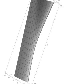
(a)

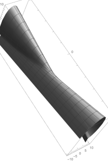
(b)

Figure 8. Two parabolic ruled surfaces. See [9].

Proposition A.2.

Assume as in Theorem 3.13. Choose $\kappa_{1}$ and $\kappa_{2}$ satisfying $0<\kappa_{1}\leq\kappa_{2}<1$. The closure of $\mathcal{H}_{s_{0},\kappa_{1},\kappa_{2}}$ under ${\mathbf{d}}_{H}$ is a compact set $\mathcal{H}_{s_{0},\kappa_{1},\kappa_{2}}\cup\{\zeta_{\left(\mkern-4.0mu\left(1,0,0,0\right)\mkern-4.0mu\right)}\}$.

Proof.

The space of open geodesic segments of ${\mathbf{d}}$-length $\pi$ in the $3$-hemisphere $\mathcal{H}$ forms a compact metric space under the Hausdorff metric ${\mathbf{d}}_{H}$. We show this by showing that every sequence of elements of $\mathcal{H}_{s_{0},\kappa_{1},\kappa_{2}}$ has an accumulation point in $\mathcal{H}_{s_{0},\kappa_{1},\kappa_{2}}$ or accumulates to ${\rm Cl}(\zeta_{\left(\mkern-4.0mu\left(1,0,0,0\right)\mkern-4.0mu\right)})$.

Given a sequence of segments $\{u_{i}\}$ in $\mathcal{H}_{s_{0},\kappa_{1},\kappa_{2}}$, $u_{i}=g^{t_{i}}(l_{i}),$ where $l_{i}\cap\mathsf{E}$ is given by

(A.2) $$l_{i}(s)=(sa_{i},y_{0,i},sc_{i})\hbox{ for }y_{0,i}\geq s_{0},a_{i},c_{i}>0,\\ \frac{\kappa_{1}a_{i}}{c_{i}}\leq\frac{y_{0,i}}{\mu}\leq\frac{\kappa_{2}a_{i}}{c_{i}},a_{i}^{2}+c_{i}^{2}=1.$$

The boundedness of one of $y_{0,i}$ or $\frac{a_{i}}{c_{i}}$ implies that of the other. If $y_{0,i}$ or $\frac{a_{i}}{c_{i}}$ is bounded above, then $l_{i}$ geometrically converges to an element of $\mathcal{H}_{s_{0},\kappa_{1},\kappa_{2}}$ up to a choice of a subsequence. If $t_{i}\rightarrow\pm\infty$, then $u_{i}\rightarrow{\zeta_{\left(\mkern-4.0mu\left(1,0,0,0\right)\mkern-4.0mu\right)}}$ since the estimates in (A.1) in the proof of Lemma A.1 hold in this case. If $t_{i}$ is bounded, then $u_{i}\rightarrow u_{0}\in\mathcal{H}_{s_{0},\kappa_{1},\kappa_{2}}$.

Hence, we are left with the case where

$$y_{0,i}\rightarrow\infty,\frac{a_{i}}{c_{i}}\rightarrow\infty,\hbox{ and }t_{i}\rightarrow\pm\infty.$$

We will show that $u_{i}\rightarrow\zeta_{\left(\mkern-4.0mu\left(1,0,0,0\right)\mkern-4.0mu\right)}$: Suppose not. Then $u_{i}$ converges to a line $u_{\infty}$ passing $\mathsf{E}$ under the metric ${\mathbf{d}}_{H}$. Then $u_{\infty}$ has the direction $(1,0,0)$ since $\left(\mkern-4.0mu\left(\mathcal{L}(\Phi_{t})(\mathbf{v})\right)\mkern-4.0mu\right)\rightarrow\left(\mkern-4.0mu\left(1,0,0\right)\mkern-4.0mu\right)$ for a generic vector $\mathbf{v}$.

By applying an element of $g^{t}$ to $u_{\infty}$ and the sequence $u_{i}$, we may assume that $u_{\infty}\cap\mathsf{E}$ is given as the line

$$x=s,y=C,z=0,s\in{\mathbb{R}}:$$

Since $u_{i}$ geometrically converges to $u_{\infty}$, $u_{i}$ intersected with $x=0$ is near $(0,C,0)$. By changing $u_{i}$ by a bounded $g^{s_{i}}$ with $s_{i}\rightarrow 0$, we may assume without loss of generality that $u_{i}$ passes $(0,C_{i},0)$ while we still have $u_{i}\rightarrow u$ under ${\mathbf{d}}_{H}$. Here $C_{i}\rightarrow C$.

By our construction, $u_{i}$ is contained in a hyperplane $P_{i}$ tangent to a parabolic cylinder $S_{i}$ given by the equation $2\mu y=z^{2}+2\mu C_{1,i}$ for some $C_{1,i}\in{\mathbb{R}}$. The line $u_{i}$ meets $S_{i}$ at the unique point $(x^{*}_{i},y^{*}_{i},z^{*}_{i})$. Project $P_{i}$ and $S_{i}$ to the $yz$-plane. Then the image of $P_{i}$ passes $(C_{i},0)$ and tangent to the parabola $2\mu y=z^{2}+2\mu C_{1,i}$. We compute by elementary geometry

$$z^{*}_{i}=\pm\sqrt{2\mu C_{1,i}-2\mu C_{i}}\hbox{ and }y^{*}_{i}=2C_{1,i}-C_{i}.$$

Now, we wish to compute $t_{i}$ so that $g^{t_{i}}(l)=u_{i}$ as in (3.13) where $l(s)$ passes $(0,C_{1,i},0)$. We compute $t$ satisfying

$$\Phi_{t}(0,C_{1,i},0)=\left(tC_{1,i}+\frac{\mu t^{3}}{3},C_{1,i}+\frac{\mu t^{2}}{2},\mu t\right)=(x^{*}_{i},y^{*}_{i},z^{*}_{i})$$

recalling (3.6). We let $t_{i}$ denote the answer

(A.3) $$y^{*}_{i}=2C_{1,i}-C_{i}=C_{1,i}+\frac{\mu t_{i}^{2}}{2}\hbox{ and }t_{i}=\pm\sqrt{\frac{2(C_{1,i}-C_{i})}{\mu}}.$$

The vector $\alpha_{i}$ tangent to $u_{i}$ is given by

$$\left(t_{i}C_{1,i}+\frac{\mu t_{i}^{3}}{6},C_{1,i}+\frac{\mu t_{i}^{2}}{2},\mu t_{i}\right)-(0,C_{i},0)$$

$$=\left(t_{i}C_{1,i}+\frac{\mu t_{i}^{3}}{6},C_{1,i}-C_{i}+\frac{\mu t_{i}^{2}}{2},\mu t_{i}\right).$$

Since the sequence of the directions of the vectors converges to $(1,0,0)$ by our assumption on $u_{i}$, we obtain $t_{i}\rightarrow\pm\infty$.

Recall

$$\mathcal{L}(\Phi_{t_{i}})^{-1}=\begin{pmatrix}1&-t_{i}&\frac{t_{i}^{2}}{2}\\ 0&1&-t_{i}\\ 0&0&1\end{pmatrix}.$$

We compute $\mathcal{L}(\Phi_{t_{i}}^{-1})(\alpha_{i})$ to be

$$\left(t_{i}C_{1,i}+\frac{\mu t_{i}^{3}}{6}-t_{i}(C_{1,i}-C_{i})-\frac{\mu t_{i}^{3}}{2}+\frac{\mu t_{i}^{3}}{2},C_{1,i}-C_{i}+\frac{\mu t_{i}^{2}}{2}-\mu t_{i}^{2},\mu t_{i}\right)\\ =\left(\frac{\mu t_{i}^{3}}{6}+t_{i}C_{i},0,\mu t_{i}\right).$$

Recall the condition (3.13) to $g^{-t_{i}}(u_{i})=l$, which yields $C_{1,i}/\mu\leq\kappa_{2}(t_{i}^{2}/6+C_{i}/\mu)$, and we obtain

$$C_{1,i}\leq\kappa_{2}\frac{1}{3}{|C_{1,i}-C_{i}|}+\kappa_{2}C_{i}\hbox{ and }\kappa_{2}<1$$

by (A.3). Since $t_{i}\rightarrow\pm\infty$, we obtain $C_{1,i}\rightarrow+\infty$ and $C_{i}\rightarrow C$. This contradicts the above inequality.

We conclude that $u_{i}$ can converge only to points of $\mathcal{H}_{s_{0},\kappa_{1},\kappa_{2}}$ or ${\zeta_{\left(\mkern-4.0mu\left(1,0,0,0\right)\mkern-4.0mu\right)}}$. This gives us a sequential convergence property. The closure of $\mathcal{H}_{s_{0},\kappa_{1},\kappa_{2}}$ is a compact metric space $\mathcal{H}_{s_{0},\kappa_{1},\kappa_{2}}\cup\{{\zeta_{\left(\mkern-4.0mu\left(1,0,0,0\right)\mkern-4.0mu\right)}}\}$.

∎

Lemma A.3.

Let $M$ be a compact metric space. Suppose that there exists a one-dimensional flow $\phi_{t}:M\rightarrow M$, $t\in{\mathbb{R}}$, with a fixed point $p$. Suppose that the orbit of every point starts and ends at $p$, and the orbit space $(M\setminus\{p\})/\sim$ is not compact. Then every $\epsilon$-ball of $p$ contains an orbit starting and ending at $p$.

Proof.

Choose a compact set $K=M\setminus B_{\epsilon}(p)$ for an open $\epsilon$-ball of $p$. Since

$$(\bigcup_{t\in{\mathbb{R}}}\phi_{t}(K))/\sim\,\,\,=K/\sim$$

is compact, and $(M\setminus\{p\})/\sim$ is not compact, it follows that

$$M\setminus\bigcup_{t\in{\mathbb{R}}}\phi_{t}(K)=\bigcap_{t\in{\mathbb{R}}}\phi_{t}(B_{\epsilon}(p))\subset B_{\epsilon}(p)$$

is not empty. Then a point here gives us an example of the closed orbit. ∎

Proof of Theorem 3.13.

We will first show that $\Psi:{\mathbb{R}}^{2}\rightarrow\mathsf{E}$ is a proper injective map.

Since $g^{t}$ acts on $P_{T^{\prime}}$ for each $T^{\prime}$, we have a self-intersection of $\Psi$ if

$$g^{t}(l(s)\cap P_{T^{\prime}})=l(s^{\prime})\cap P_{T^{\prime}}\hbox{ for some }t>0,s,s^{\prime}\in{\mathbb{R}}\hbox{ and }T^{\prime}\in{\mathbb{R}}.$$

The following hold:

• $l(s)\cap P_{T^{\prime}}$ is a pair of points provided $T^{\prime}>-2\mu y_{0}$, or

• $T^{\prime}=-2\mu y_{0}$ and $l(s)\cap P_{T^{\prime}}$ is $(0,y_{0},0)$, or else

• $l(s)\cap P_{T^{\prime}}$ is empty for $T^{\prime}<-2\mu y_{0}$.

Thus, only in the first case, we can have a self-intersection of the image of $\Psi$ under the quotient space $\mathsf{E}/\langle g\rangle$. Now $l(s)\cap P_{T^{\prime}}$ can be computed as follows :

$$(sc)^{2}-2\mu y_{0}=T^{\prime}\hbox{ and }s_{0}=\sqrt{T^{\prime}+2\mu y_{0}}/c$$

and the points are $(\pm s_{0}a,y_{0},\pm s_{0}c)$. And we obtain

$$F_{3}(\pm s_{0}a,y_{0},\pm s_{0}c)=\pm(s_{0}^{3}c^{3}-3\mu y_{0}s_{0}c+3\mu^{2}s_{0}a).$$

These are distinct unless the value is $0$. Since $F_{3}$ is invariant under $g$, it follows that if $F_{3}$-values of two points are distinct, then they cannot be in the same orbit of $\langle g\rangle$. If $F_{3}=0$, we must have

$$\frac{a}{c}=-\frac{T^{\prime}}{3\mu^{2}}+\frac{y_{0}}{3\mu}.$$

Since $-T^{\prime}<2\mu y_{0}$, we obtain

(A.4) $$\frac{a}{c}<\frac{2\mu y_{0}}{3\mu^{2}}+\frac{y_{0}}{3\mu}=\frac{y_{0}}{\mu}.$$

Thus, if we choose $y_{0}<\mu\frac{a}{c}$, the self-intersection of $\Psi$ never happens. For example, choosing $y_{0}$ sufficiently small or choosing $\frac{a}{c}$ sufficiently large would satisfy the condition. This proves the injectivity of $\Psi$.

By (3.7), $g^{t}$ acts properly on each parabolic cylinder $P_{T}$ since $F_{1}$ and $F_{2}$ are invariants of the vector field on $\phi$, and each intersection of $F_{1}\cap F_{2}$ is a complete flow line.

We now prove the properness of $\Psi$. Suppose that there is a compact set $K\subset\mathsf{E}$ and $g^{t_{i}}(l)\cap K$ is not empty for a sequence $\{t_{i}\}$ of real numbers such that $t_{i}\rightarrow\infty$. (The case when $t_{i}\rightarrow-\infty$ is entirely similar.) However, $K$ is in the region $B$ in $\mathsf{E}$ bounded by two parabolic cylinders $P_{T_{1}}$ and $P_{T_{2}}$ for some pair $T_{1}$ and $T_{2}$. Then $l$ meets $P_{T_{j}},j=1$ at most two points. If $l$ does not meet $B$, then $g^{t}(l)$, $t\in{\mathbb{R}}$ is disjoint from $K$ since the region bounded by $P_{T_{j}}$ is $g^{t}$-invariant. If $l\cap B\neq\emptyset$,

$$g^{t_{i}}(l\cap B)\rightarrow\{\left(\mkern-4.0mu\left(1,0,0,0\right)\mkern-4.0mu\right)\}\,\,\hbox{ or }\{\left(\mkern-4.0mu\left(-1,0,0,0\right)\mkern-4.0mu\right)\}\,\,\hbox{ as }t_{i}\rightarrow\pm\infty$$

by convexity since the endpoints of $l\cap B$ do this. This proves the properness of $\Psi:{\mathbb{R}}^{2}\rightarrow\mathsf{E}$ and that $g^{t_{i}}(l)$ can have limit points only in ${\mathbb{S}}$.

The first item is proved by Lemma A.1.

Choose $\kappa_{1}$ and $\kappa_{2}$ satisfying $0<\kappa_{1}\leq\kappa_{2}<1$. There is a continuous map $\iota_{R}:\mathcal{H}_{s_{0},\kappa_{1},\kappa_{2}}\rightarrow{\mathbb{S}}_{+}$ by taking the endpoints in ${\mathbb{S}}_{+}$. The image is a horodisk $\mathcal{E}$. Since $\mathcal{E}/\sim$ is not compact, $\mathcal{H}_{s_{0},\kappa_{1},\kappa_{2}}/\sim$ is not compact under the orbit equivalence relation under $g^{t},t\in{\mathbb{R}}$

By Proposition A.2, $\mathcal{H}_{s_{0},\kappa_{1},\kappa_{2}}\cup\{{\zeta_{\left(\mkern-4.0mu\left(1,0,0,0\right)\mkern-4.0mu\right)}}\}$ is compact. In any $\epsilon$-${\mathbf{d}}_{H}$-neighborhood $\hat{N}$, $\epsilon>0$, of ${\rm Cl}(\zeta_{\left(\mkern-4.0mu\left(1,0,0,0\right)\mkern-4.0mu\right)})$ in $\mathcal{H}_{s_{0},\kappa_{1},\kappa_{2}}$, we can find a $g^{t}$-orbit in $\hat{N}$ by Lemma A.3. Take any neighborhood $N$ of ${\rm Cl}(\zeta_{\left(\mkern-4.0mu\left(1,0,0,0\right)\mkern-4.0mu\right)})$ in ${\mathbb{S}}^{3}$. Since we are using the Hausdorff metric, we can find an $\epsilon$-${\mathbf{d}}_{H}$-neighborhood $\hat{N}$ in $\mathcal{H}_{s_{0},\kappa_{1},\kappa_{2}}\cup\{{\zeta_{\left(\mkern-4.0mu\left(1,0,0,0\right)\mkern-4.0mu\right)}}\}$ so that any segment in $\hat{N}$ is a segment in $N$. Then the $g^{t}$-orbit as above will give us the desired ruled surface in $N$. This proves the second item.

The first and second items imply the fact on the boundary of $S_{f,r}$. Clearly,$S_{f,r}$ bounds a domain in $\mathsf{E}$ with boundary ${\rm Cl}(S_{f,r})$. This domain is homeomorphic to a $3$-cell by Lemma 1.12 of [36]. Also, $g$ sends the disk leaves of the foliation $\mathcal{D}_{f,r_{0}}$ of the domain to a disjoint disk leaf in Theorem 3.14. Hence, the quotient space is homeomorphic to a solid torus. ∎

A.2. Two transversal foliations

Proof of Theorem 3.14.

The fact that $S_{f,r}$ is a properly embedded surface is proved in Theorem 3.13. We defined $l_{f,r}(s)=(sr,f(\rho),s\sqrt{1-r^{2}})$. We define

$$l_{f}:[r_{0},1)\times{\mathbb{R}}\rightarrow\mathsf{E}\hbox{ given by }l_{f}(r,s)=(sr,f(\rho),s\sqrt{1-r^{2}}).$$

Let $u_{l_{f,r}}$ denote the vector field $(r,0,\sqrt{1-r^{2}})$ tangent to $l_{f,r}(s)$. Also, the vector field $\phi$ generating $g^{t}$ is given by $(y,z,\mu)$.

$$\frac{\partial l_{f}}{\partial r}=Y_{f}=\left(s,f^{\prime}(\rho),\frac{-sr}{\sqrt{1-r^{2}}}\right)$$

is tangent to $D_{f,r_{0},0}$ obtained by taking a tangent vector along the direction of $\frac{\partial}{\partial r}$. A triple product of three vectors is the volume of the span of three vectors in $\mathsf{E}$. We compute the triple product on the line $l_{f,r}$

(A.5) $$(u_{l_{f,r}},Y_{f},\phi)=\sqrt{1-r^{2}}\left(\frac{\mu r}{\sqrt{1-r^{2}}}-f(\rho)\right)f^{\prime}(\rho)+s^{2}>0,$$

which follows by our condition on $f$ and $r$. It follows that $u_{l_{f,r}},Y_{f},\phi$ form always an independent frame in the standard orientation on $l_{f,r}$, and so are their images under $g^{t}$ since $g^{t}$ is volume-preserving. Thus,

$$Dg^{t}(u_{l_{f,r}}),Dg^{t}(Y_{f}),Dg^{t}(\phi)$$

form an independent frame at each point of $S_{f,r}$.

We claim that $S_{f,r}$ is disjoint from $S_{f,r^{\prime}}$ for $r_{0}\leq r<r^{\prime}<1$: By (A.5), $Y_{f}$ is transversal to $S_{f,r}$ on $l_{f,r}$. We define the vector field $Y_{f}$ on $S_{f,r}$ so that

$$Y_{f}(g^{t}(sr,f(\rho),s\sqrt{1-r^{2}}))=Dg^{t}(Y_{f}(sr,f(\rho),s\sqrt{1-r^{2}})).$$

The extended $Y_{f}$ is transversal to $S_{f,r}$ since the triple product is invariant under the Lorentzian isometries. Define $\Xi_{f}(r,t,s)=g^{t}(l_{f}(r,s)))$, which gives us a parametrization of $S_{f,r}$. We obtain the partial derivative with respect to $r$ by chain-rules:

$$\frac{\partial{\Xi_{f}(r,t,s)}}{\partial r}=Dg^{t}(Y_{f}(l_{f}(r,s)))=Y_{f}(\Xi_{f}(r,t,s)).$$

Solving the following ordinary differential equation with respect to the variable $r$

$$\frac{\partial\Xi_{f}(r,t,s)}{\partial r}=Y_{f}(\Xi_{f}(r,t,s))$$

gives us a flow $\Xi_{f}(r,t,s)$ for $r$ in some interval with fixed $t,s$. Using the quasi-linear Cauchy theorem (Theorem 9.52 of [35]) and the transversality, we obtain the disjointness.

Also, for each point $x$ of $R_{f,r_{0}}$, there is a leaf $S_{f,r^{\prime}}$ containing it: Let $x_{i}$ be a sequence converging to $x$ and $x_{i}\in S_{f,r_{i}}$, $r_{i}>r_{0}$. Then let $L_{i}$ be the line in $S_{f,r_{i}}$ containing $x_{i}$. Since we showed that $\mathcal{H}_{s_{0},\kappa_{1},\kappa_{2}}\cup{\rm Cl}(\zeta_{\left(\mkern-4.0mu\left(1,0,0,0\right)\mkern-4.0mu\right)})$ is compact by Proposition A.2, ${\rm Cl}(L_{i})$ geometrically converges to an element of $\mathcal{H}_{s_{0},\kappa_{1},\kappa_{2}}$ or to ${\rm Cl}(\zeta_{\left(\mkern-4.0mu\left(1,0,0,0\right)\mkern-4.0mu\right)})$ by choosing a subsequence if necessary. Proposition A.2 shows that $L_{i}=g^{t_{i}}(l_{f}(r_{i}))$ for bounded $t_{i}$ in the first case. Hence, $x$ is in $S_{f,\lim_{i}r_{i}}$. In the other case, $x_{i}$ does not have $x$ as a limit. This proves the closedness of the foliated subset in $R_{f,r_{0}}$.

Using the flows, we can prove the openness of the set $\bigcup_{r_{0}\leq r<1}S_{f,r^{\prime}}$. Hence, $R_{f,r_{0}}$ is foliated by leaves $S_{f,r}$, $r\geq r_{0}$.

Since each line in $D_{f,r_{0},0}$ lies on a different plane given by equations of the form $y=c$, $D_{f,r_{0},0}$ is an embedded surface, and so are $D_{f,r_{0},t}$. Proposition A.2 implies that $D_{f,r_{0},0}$ is properly embedded since ${\rm Cl}(l_{f,r_{i}})$ geometrically converges to ${\rm Cl}(\zeta_{\left(\mkern-4.0mu\left(1,0,0,0\right)\mkern-4.0mu\right)})$ as $r_{i}\rightarrow 1$. Hence, $D_{f,r_{0},t}$ is properly embedded for all $t$.

Since $g^{t_{0}}$ is generated by a vector field $\phi$ transversal to $D_{f,r_{0},t}$ for every $t$ by the above paragraph, the images under the flows of $D_{f,r_{0},t}$ are disjoint from $D_{f,r_{0},t}$. Also, $g^{t_{0}}(D_{f,r_{0},t})=D_{f,r_{0},t+t_{0}}$ follows by our above definition of $D_{f,r_{0},t}$.

Also, $R_{f,r_{0}}$ is foliated by leaves of the form $D_{f,r_{0},t}$ as follows: $\bigcup_{t\in{\mathbb{R}}}D_{f,r_{0},t}$ is open since we can use the flow generated by $g^{t}$. The closedness follows by Proposition A.2 again as above.

Now, we have a foliation by leaves of the form $S_{f,r}$ for $r\in[r_{0},1)$. Then $D_{f,r_{0},t}\cap S_{f,r}$ contains a geodesic given by $g^{t}(l(s)),s\in{\mathbb{R}}$. At $t=0$, the tangent space of $D_{f,r_{0},0}$ is generated by $u_{l},Y_{f}$, and that of $S_{f,r}$ is generated by $u_{l},\phi$. The independence above implies the transversality of $D_{f,r_{0},0}$ and $S_{f,r}$. Thus, the transversality of $D_{f,r_{0},t}$ and $S_{f,r}$ follows.

∎

Remark A.1.

There seems to be a vast literature on ruled surfaces on which a one-parameter Lorentzian isometry group acts but there seems to be no article on the topological properties. See Dillen-Kühlen [21] for a survey of geometric aspects.

Appendix B The flat ${\mathbb{R}}^{2,1}$-bundle valued $1$-forms on a cusp neighborhood

Only prerequisites are Sections 2 and 3.1 and the notation in Section 4, in particular Definition 4.1.

B.1. Replacing forms by standard cusp $1$-forms in the cusp neighborhoods

Suppose that $\Gamma$ is a discrete Lorentzian isometry group so that $\Gamma$ is a Fuchsian group acting on ${\mathbb{S}}_{+}$ with a parabolic element $g$ fixing $p\in\partial{\mathbb{S}}_{+}$. Let ${\mathsf{S}}:={\mathbb{S}}_{+}/\Gamma$ be a complete hyperbolic surface with a cusp neighborhood $E$. $E$ is covered by a horodisk $P\subset{\mathbb{S}}_{+}$ with $p\in{\rm bd}_{{\mathbb{S}}}P$. Then $P/\langle g\rangle$ is isometric to $E$.

We recall the vector bundle $\mathscr{V}$ given as the quotient of $\widetilde{\mathscr{V}}={\mathbb{S}}_{+}\times{\mathbb{R}}^{2,1}$ with action given by

$$\gamma(x,\mathbf{v})=(\gamma(x),\mathcal{L}(\gamma)(\mathbf{v}))\hbox{ for }\gamma\in\Gamma,\mathbf{v}\in{\mathbb{R}}^{2,1}.$$

Recall (4.7) that for $\widetilde{\mathscr{V}}$-valued $1$-forms on ${\mathbb{S}}_{+}$, the action is given by

$$\gamma^{*}(\mathbf{v}\otimes dx)=\mathcal{L}(\gamma)^{-1}(\mathbf{v})\otimes dx\circ\gamma.$$

Proposition B.1.

Let ${\mathsf{S}}$, $\Gamma$, $P$, $E$, and $\gamma$ be as above in Section B.1. Let $\eta$ be a closed $\mathscr{V}$-valued $1$-form representing a class in $H^{1}({\mathsf{S}},\mathscr{V})$. Let $\zeta$ be a closed $\mathscr{V}$-valued $1$-form in $E$ so that $\zeta$ is cohomologous to $\eta|E$ in $H^{1}(E,\mathscr{V})$. Then we can find a closed $\mathscr{V}$-valued $1$-form $\eta^{\prime}$ on ${\mathsf{S}}$ cohomologous to $\eta$ and a cusp neighborhood $E^{\prime}\subset E$ so that $\eta^{\prime}|E^{\prime}=\zeta|E^{\prime}$.

Proof.

Let $E^{\prime}\subset E$ be a smaller cusp neighborhood so that ${\rm Cl}(E^{\prime})\subset E$. Consider $\eta-\zeta$ on $E^{\prime}$. Then $\eta-\zeta=df$ for a section $f:E^{\prime}\rightarrow\mathscr{V}$. We can extend $f$ to a smooth section $f:{\mathsf{S}}\rightarrow\mathscr{V}$ by a partition of unity so that $f=0$ on ${\mathsf{S}}\setminus E$. Then define $\eta^{\prime}=\eta$ on ${\mathsf{S}}\setminus E$ and $\eta^{\prime}=\zeta$ on $E^{\prime}$ and $\eta^{\prime}=\eta-df$ on $E\setminus E^{\prime}$. ∎

Proposition B.2.

$H^{1}(E,\mathscr{V})={\mathbb{R}}$.

Proof.

Recall that $E$ is homotopy equivalent to ${\mathbb{S}}^{1}$. Thus, $\pi_{1}(E)$ is an infinite cyclic group. $\mathscr{V}|E$ is $P\times{\mathbb{R}}^{2,1}/\langle g\rangle$. Recall that $\mathcal{L}(g)={\rm I}+N(g)+N(g)^{2}/2$ for a nilpotent matrix $N(g)$ of rank 2 from (3.6). We conclude using the knowledge of Section 3 of [29]:

$$Z^{1}(\langle g\rangle,\mathscr{V}) =\{\mathbf{v}:{\mathbb{Z}}\rightarrow{\mathbb{R}}^{2,1}|\mathcal{L}(g^{i})\mathbf{v}(g^{j})-\mathbf{v}(g^{i+j})=0\,\forall i,j\in{\mathbb{Z}}\}\cong{\mathbb{R}}^{2,1},$$

$$B^{1}(\langle g\rangle,\mathscr{V}) =\{\mathbf{v}:{\mathbb{Z}}\rightarrow{\mathbb{R}}^{2,1}|\mathbf{v}(g)=\mathcal{L}(g)\mathbf{v}_{0}-\mathbf{v}_{0},\mathbf{v}_{0}\in{\mathbb{R}}^{2,1}\},$$

$$=N(g)\left(\left({\rm I}+\frac{1}{2}N(g)\right)({\mathbb{R}}^{2,1})\right)=N(g)({\mathbb{R}}^{2,1}),$$

(B.1) $$H^{1}(\langle g\rangle,\mathscr{V}) ={\mathbb{R}}^{2,1}/N(g)({\mathbb{R}}^{2,1})\cong{\mathbb{R}}.$$

The second to last equation follows since $I+N(g)/2$ is invertible. The last follows since $N(g)$ is of rank two by Section 3.1. ∎

B.2. The integral of the standard cusp $1$-form

We will use the notation of Section 4.4. Let $P$ be the standard horodisk in ${\mathbb{S}}_{+}$ with $\mathbf{p}$ as a null vector in the direction of ${\rm Cl}(P)\cap\partial{\mathbb{S}}_{+}$. The standard cusp $1$-form for $P$ is given where $P$ is given by $y>1$ in the upper half-space model ${\mathsf{U}}^{2}$ of the hyperbolic plane. A geodesic in $P$ is given by equation $(x\pm R)^{2}+y^{2}=R^{2}$ in ${\mathsf{U}}^{2}$ and parameterized by $\zeta(\theta):=(R\cos\theta\mp R,R\sin\theta)$. The starting point and the endpoint are given by $R\sin\theta=1$. Thus, the beginning $\theta_{0}$ and ending $\theta_{1}=\pi-\theta_{0}$ is one of the values of $\sin^{-1}(\frac{1}{R})$.

We assume that a complete geodesic $l$ passes a cusp region with the cusp point $p=\left(\mkern-4.0mu\left(\mathbf{p}\right)\mkern-4.0mu\right)$ and the standard cusp $1$-form. We assume that by choice of the coordinates of ${\mathsf{U}}^{2}$, $p=\infty$ and the geodesic starts at $(0,0)$ and ends at $(2R,0)$ or at $(-2R,0)$. We say that $l$ and any horizontal translation of $l$ in the upper half model have radius $R$.

There is an isometry $H:{\mathsf{U}}^{2}\rightarrow{\mathbb{S}}_{+}$ to the Klein model ${\mathbb{S}}_{+}$:

$$H(x,y):=\left(\mkern-4.0mu\left(\overrightarrow{H(x,y)}\right)\mkern-4.0mu\right)\hbox{ where }\overrightarrow{H(x,y)}:=\left(\frac{2x}{x^{2}+y^{2}+1},1-\frac{2}{x^{2}+y^{2}+1},1\right),$$

(See Theorem 7.1 of Hongchan Kim [33].) This extends to the boundary $y=0$ and induces a homeomorphism from ${\mathsf{U}}^{2}\cup\{\infty\}$ to the closure of the unit disk where $\infty$ goes to $\left(\mkern-4.0mu\left(\mathbf{j}+\mathbf{k}\right)\mkern-4.0mu\right)$.

The standard horodisk in ${\mathsf{U}}^{2}$ is given by $y>1$. The image of this under $H$ is the standard horodisk $Q$ of the Klein model. The standard horodisk has the point $\left(\mkern-4.0mu\left(\mathbf{j}+\mathbf{k}\right)\mkern-4.0mu\right)$ of ${\mathbb{S}}_{+}$ in the boundary and $\partial_{h}Q\ni\left(\mkern-4.0mu\left(\mathbf{k}\right)\mkern-4.0mu\right)$.

This makes things simpler.

Lemma B.3.

Let $g$, $l$, and $\left|\mkern-2.0mu\left|\cdot\right|\mkern-2.0mu\right|_{E}$ be as above. Let $D$ be the standard horodisk. Set

$$\mathbf{v}(x)=\left(x,-\frac{x^{2}}{2\sqrt{2}}+\frac{1}{\sqrt{2}},\frac{x^{2}}{2}+\frac{1}{\sqrt{2}}\right)\hbox{ for }x\in{\mathbb{R}}.$$

Let $l$ be a complete geodesic passing $D$ of radius $R$ and starts at $H(0,0)$ and ends at $H(\pm 2R,0)$. Assume $R>1$. Suppose that $l$ corresponds in ${\mathbb{S}}_{+}$ to the geodesic passing a point of $\partial_{h}D$ in the direction of a unit vector ${\mathbf{u}}$ away from $H(0,0)\in{\partial{\mathsf{U}}^{2}}$. Then the following hold:

• for any point $z$ on $l$ with coordinate $x$ in the upper half-space model,

  (B.2) $$\left|\mkern-2.0mu\left|\Pi_{\tilde{\mathbf{V}}_{0}(z,{\mathbf{u}})}(\mu\mathbf{v}(x))\right|\mkern-2.0mu\right|_{E}=\left|{\mu}\left(x-\frac{\pm\sqrt{2}}{R}\right)\right|$$

  for the cusp coefficient $\mu$, and

• (B.3) $$\left|\mkern-2.0mu\left|\Pi_{\tilde{\mathbf{V}}_{-}(z,{\mathbf{u}})}(\mu\mathbf{v})\right|\mkern-2.0mu\right|_{E}=\left|\frac{\mu\left(4R^{2}+1\right)}{4\sqrt{2}R^{2}}\right|\hbox{ and }\\ \left|\mkern-2.0mu\left|\Pi_{\tilde{\mathbf{V}}_{+}(z,{\mathbf{u}})}(\mu\mathbf{v})\right|\mkern-2.0mu\right|_{E}=\left|{\mu}\left(\frac{1}{4\sqrt{2}R^{2}}-\frac{\pm x}{2R}+\frac{x^{2}}{2\sqrt{2}}\right)\right|$$

Proof.

These are simple computations using $H$, and the used frames there form uniformly bounded matrices in ${\mathsf{GL}}(3,{\mathbb{R}})$. Hence, the estimations are uniformly compatible with the standard Euclidean metric results. (See [12] and [13].) ∎

Let $\zeta=l\cap D$ be a geodesic segment with both endpoints in $\partial_{h}D$. Suppose that $l$ is in the form of Lemma B.3 parameterized by the angle $\theta$ from the center of the semicircle in the upper-half-space model containing $l$. Also, recall the geodesic flow $\Psi_{t}$ acting on ${\mathbb{R}}^{2,1}\times\mathsf{U}{\mathbb{S}}_{+}$ from Section 3.2. We reparametrize $l$ by $\Psi(z,\theta)$ for $z$ the beginning point of $\zeta$ and $\theta\in(0,\pi)$ with $z=\Psi(z,\theta_{0})$. Let $\eta$ denote the standard $1$-form defined on $D$. We define

$$\mathbf{b}(\zeta):=\,\int_{\theta_{0}}^{\pi-\theta_{0}}{\mathbb{D}}\Psi(z,\theta-\theta_{0})^{-1}\left(\eta\left(\frac{d\Psi(z,\theta)}{d\theta}\right)\right)d\theta,$$

where $\theta_{0}$ and $\pi-\theta_{0}$ are the start and the end angles of the semicircle $l$ parameterized by angles.

We recall $\mathbf{b}_{\pm}(\zeta)$ from (4.29) as the $\tilde{V}_{\pm}$-component of $\mathbf{b}(\zeta)$: that is,

$$\mathbf{b}_{\pm}(\zeta):=\,\int_{\theta_{0}}^{\pi-\theta_{0}}\Pi_{\tilde{V}_{\pm}}\left({\mathbb{D}}\Psi(z,\theta-\theta_{0})^{-1}\left(\eta\left(\frac{d\Psi(z,\theta)}{d\theta}\right)\right)\right)d\theta.$$

We define

(B.4) $$\alpha(\zeta):=\int{\mathsf{B}}\left({\mathbf{\nu}},\eta\left(\frac{d\Psi(z,\theta)}{d\theta}\right)\right)d\theta.$$

Proposition B.4.

Let $g$, $l$, and $\left|\mkern-2.0mu\left|\cdot\right|\mkern-2.0mu\right|_{E}$ be as above. Let $D$ be the standard horodisk. Let $\eta$ be a standard cusp $1$-form for a cusp constant $\mu{\color[rgb]{0,0,0}>0}$. (See (4.18). ) Suppose that a complement geodesic $l$ of radius $R$ is in the form of Lemma B.3. Let $\zeta=l\cap D$ be a geodesic segment with both endpoints in $\partial_{h}D$. Then we obtain

(B.5) $$\left|\mkern-2.0mu\left|\mathbf{b}_{-}(\zeta)\right|\mkern-2.0mu\right|_{E}=\mu\frac{\sqrt{-1+R^{2}}(1+4R^{2})}{2\sqrt{2}R^{2}}\leq\frac{5}{2\sqrt{2}}\mu R,\\ \mu\left(-\sqrt{2}+2R^{2}\right)\frac{\sqrt{-1+R^{2}}}{R}\leq\alpha(\zeta)=\mu\frac{\sqrt{-1+R^{2}}}{R}(\pm\sqrt{2}+2R^{2})\leq\mu(\sqrt{2}+2R^{2})$$

where $R\geq 1$.

Proof.

In this case, we may regard ${\mathbb{D}}\Psi(z,\theta)^{-1}$ as the identity since we will work directly over ${\mathbb{S}}_{+}$ (see Remark 4.1): Since the projection $\Pi_{\tilde{V}_{-}}$ to $\tilde{V}_{-}$ commutes with ${\mathbb{D}}\Psi(z,\theta)^{-1}$,

$$\mathbf{b}_{-}(\zeta):=\,\int_{\theta_{0}}^{\pi-\theta_{0}}{\mathbb{D}}\Psi(z,\theta)^{-1}\left(\Pi_{\tilde{V}_{-}}(\eta)\right)dx\left(\frac{d\Psi(z,\theta)}{d\theta}\right)d\theta.$$

By computations in [12] or [13], we obtain

$$\left|\mkern-2.0mu\left|\mathbf{b}_{-}(\zeta)\right|\mkern-2.0mu\right|=\mu\sqrt{-1+R^{2}}\frac{(1+4R^{2})}{2\sqrt{2}R^{2}}.$$

And we evaluate the contribution of $l\cap P$ to $\mathbf{b}_{0}$ :

$$\alpha(\zeta)=\mu\left(\sqrt{-1+R^{2}})(\pm\sqrt{2}+2R^{2})\right)/R.$$

∎

References

- [1] James W. Anderson, Petra Bonfert-Taylor, and Edward C. Taylor. Convergence groups, Hausdorff dimension, and a theorem of Sullivan and Tukia. Geom. Dedicata, 103:51–67, 2004.
- [2] Alan F. Beardon. The geometry of discrete groups, volume 91 of Graduate Texts in Mathematics. Springer-Verlag, New York, 1983.
- [3] Alan F. Beardon and Bernard Maskit. Limit points of Kleinian groups and finite sided fundamental polyhedra. Acta Math., 132:1–12, 1974.
- [4] Riccardo Benedetti and Carlo Petronio. Lectures on hyperbolic geometry. Universitext. Springer-Verlag, Berlin, 1992.
- [5] Richard D. Canary and Yair N. Minsky. On limits of tame hyperbolic -manifolds. J. Differential Geom., 43(1):1–41, 1996.
- [6] Virginie Charette and Todd A. Drumm. The Margulis invariant for parabolic transformations. Proc. Amer. Math. Soc., 133(8):2439–2447, 2005.
- [7] Virginie Charette and Youngju Kim. Foliations of Minkowski spacetime by crooked planes. Internat. J. Math., 25(9):1450088, 25, 2014.
- [8] Suhyoung Choi. Calculus-v2.nb. Mathematica™ file at mathsci.kaist.ac.kr/~schoi/research.html.
- [9] Suhyoung Choi. convergenceII-v2.nb. Mathematica™ file at mathsci.kaist.ac.kr/~schoi/research.html.
- [10] Suhyoung Choi. FoliationsV2.nb. Mathematica™ file at mathsci.kaist.ac.kr/~schoi/research.html.
- [11] Suhyoung Choi. gedesicFinal-v2.nb. Mathematica™ file at mathsci.kaist.ac.kr/~schoi/research.html.
- [12] Suhyoung Choi. NewNormalComp-v3.nb. Mathematica™ file at mathsci.kaist.ac.kr/~schoi/research.html.
- [13] Suhyoung Choi. NewNormalComp2-v3.nb. Mathematica™ file at mathsci.kaist.ac.kr/~schoi/research.html.
- [14] Suhyoung Choi. StandardFormII-v4.nb. Mathematica™ file at mathsci.kaist.ac.kr/~schoi/research.html.
- [15] Suhyoung Choi. Vanalysis-v2.nb. Mathematica™ file at mathsci.kaist.ac.kr/~schoi/research.html.
- [16] Suhyoung Choi and William Goldman. Topological tameness of Margulis spacetimes. Amer. J. Math, 139:297–345, 2017. ArXiv:1204.5308.
- [17] Jeffrey Danciger, François Guéritaud, and Fanny Kassel. Margulis spacetimes with parabolic elements. in preparation.
- [18] Jeffrey Danciger, François Guéritaud, and Fanny Kassel. Fundamental domains for free groups acting on anti-de Sitter 3-space. Math. Res. Lett., 23(3):735–770, 2016.
- [19] Jeffrey Danciger, François Guéritaud, and Fanny Kassel. Geometry and topology of complete Lorentz spacetimes of constant curvature. Ann. Sci. Éc. Norm. Supér. (4), 49(1):1–56, 2016.
- [20] Jeffrey Danciger, François Guéritaud, and Fanny Kassel. Margulis spacetimes via the arc complex. Invent. Math., 204(1):133–193, 2016.
- [21] Franki Dillen and Wolfgang Kühnel. Curvature of ruled surfaces and groups of Lorentzian motions. In Geometry and topology of submanifolds, IX (Valenciennes/Lyon/Leuven, 1997), pages 135–138. World Sci. Publ., River Edge, NJ, 1999.
- [22] Todd A. Drumm. Fundamental polyhedra for Margulis space-times. Topology, 31(4):677–683, 1992.
- [23] D. B. A. Epstein and A. Marden. Convex hulls in hyperbolic space, a theorem of Sullivan, and measured pleated surfaces [mr0903852]. In Fundamentals of hyperbolic geometry: selected expositions, volume 328 of London Math. Soc. Lecture Note Ser., pages 117–266. Cambridge Univ. Press, Cambridge, 2006.
- [24] David B. A. Epstein and Carlo Petronio. An exposition of Poincaré’s polyhedron theorem. Enseign. Math. (2), 40(1-2):113–170, 1994.
- [25] Sourav Ghosh and Nicholaus Treib. Affine anosov representations and proper actions. arXiv:1711.09712.
- [26] William Goldman and Morris W. Hirsch. The radiance obstruction and parallel forms on affine manifolds. Trans. Amer. Math. Soc., 286(2):629–649, 1984.
- [27] William M. Goldman. Projective structures with Fuchsian holonomy. J. Differential Geom., 25(3):297–326, 1987.
- [28] William M. Goldman and François Labourie. Geodesics in Margulis spacetimes. Ergodic Theory Dynam. Systems, 32(2):643–651, 2012.
- [29] William M. Goldman, François Labourie, and Gregory Margulis. Proper affine actions and geodesic flows of hyperbolic surfaces. Ann. of Math. (2), 170(3):1051–1083, 2009.
- [30] C. McA. Gordon and R. A. Litherland. Incompressible surfaces in branched coverings. In The Smith conjecture (New York, 1979), volume 112 of Pure Appl. Math., pages 139–152. Academic Press, Orlando, FL, 1984.
- [31] Ernst Heintze and Hans-Christoph Im Hof. Geometry of horospheres. J. Differential Geometry, 12(4):481–491 (1978), 1977.
- [32] John Hempel. 3-manifolds. AMS Chelsea Publishing, Providence, RI, 2004. Reprint of the 1976 original.
- [33] Hong Chan Kim. Embedding of the Teichmüller space into the Goldman space. J. Korean Math. Soc., 43(6):1231–1252, 2006.
- [34] François Labourie. Lectures on representations of surface groups. Zurich Lectures in Advanced Mathematics. European Mathematical Society (EMS), Zürich, 2013.
- [35] John M. Lee. Introduction to Riemannian manifolds, volume 176 of Graduate Texts in Mathematics. Springer, Cham, 2018. Second edition of [ MR1468735].
- [36] Albert Marden. The geometry of finitely generated Kleinian groups. Ann. of Math. (2), 99:383–462, 1974.
- [37] Albert Marden. Outer circles. Cambridge University Press, Cambridge, 2007.
- [38] Albert Marden. Hyperbolic manifolds. Cambridge University Press, Cambridge, 2016.
- [39] G. A. Margulis. Free completely discontinuous groups of affine transformations. Dokl. Akad. Nauk SSSR, 272(4):785–788, 1983.
- [40] G. A. Margulis. Complete affine locally flat manifolds with a free fundamental group. Zap. Nauchn. Sem. Leningrad. Otdel. Mat. Inst. Steklov. (LOMI), 134:190–205, 1984. Automorphic functions and number theory, II.
- [41] James R. Munkres. Topology: a first course. Prentice-Hall, Inc., Englewood Cliffs, N.J., 1975.
- [42] Kenichi Ohishka. Oral communications, 1997.
- [43] Peter Scott and Thomas Tucker. Some examples of exotic noncompact -manifolds. Quart. J. Math. Oxford Ser. (2), 40(160):481–499, 1989.
- [44] Ilia Smilga. Proper affine actions: a sufficient criterion. to appear in Math. Annalen, arXiv:1612.08942.
- [45] Ilia Smilga. Proper affine actions on semisimple Lie algebras. Ann. Inst. Fourier (Grenoble), 66(2):785–831, 2016.
- [46] Ilia Smilga. Proper affine actions in non-swinging representations. Groups Geom. Dyn., 12(2):449–528, 2018.
- [47] William Thurston. Geometry and topology of -manifolds. Lecture notes, Princeton University, 1984, http://www.msri.org/publications/books/gt3m/.
- [48] Pekka Tukia. Conical limit points and uniform convergence groups. J. Reine Angew. Math., 501:71–98, 1998.