Phonon-particle coupling effects in odd-even mass differences of semi-magic nuclei.Phonon-particle coupling effects in odd-even mass differences of semi-magic nuclei. E. E. Saperstein, M. Baldo, S. S. Pankratov, S. V. Tolokonnikov E. E. Saperstein, M. Baldo, S. S. Pankratov, S. V. Tolokonnikov *

Phonon-particle coupling effects in odd-even mass differences of semi-magic nuclei.

Abstract

A method to evaluate the particle-phonon coupling (PC) corrections to the single-particle energies in semi-magic nuclei, based on a direct solving the Dyson equation with PC corrected mass operator, is used for finding the odd-even mass difference between 18 even Pb isotopes and their odd-proton neighbors. The Fayans energy density functional (EDF) DF3-a is used which gives rather high accuracy of the predictions for these mass differences already on the mean-field level, with the average deviation from the existing experimental data equal to 0.389 MeV. It is only a bit worse than the corresponding value of 0.333 MeV for the Skyrme EDF HFB-17 which belongs to a family of Skyrme EDFs with the highest overall accuracy in describing the nuclear masses. Account for the PC corrections induced by the low-laying phonons $2^{+}_{1}$ and $3^{-}_{1}$ significantly diminishes the deviation of the theory from the data till 0.218 MeV.

21.60.-n; 21.65.+f; 26.60.+c; 97.60.Jd

The single-particle (SP) spectrum of a nucleus essentially influences different nuclear properties. Therefore ability to describe nuclear SP spectra correctly is very important for any self-consistent nuclear theory. Till now, experimental SP levels are known in detail only for magic nuclei [1]. Their analysis in [2] on the base of the energy density functional (EDF) DF3-a [3], which is a small modification of the original Fayans EDF DF3 [4, 5], led to rather good description of the data, significantly better than the predictions of the popular Skyrme EDF HFB-17 [6] which belongs to the family of the EDFs HFB-17 – HFB-27 [7] possessing the highest accuracy among all the self-consistent calculations in reproducing nuclear masses.

Inclusion of the particle-phonon coupling (PC) corrections, with account for the non-pole diagrams [8, 9], made the agreement even better. So-called $g_{L}^{2}$-approximation for the PC corrections was applied, $g_{L}$ being the creation vertex of the $L$-phonon. The corresponding diagrams for the PC correction $\delta\Sigma^{\rm PC}_{L}$ to the mass operator $\Sigma_{0}$, in the representation of the SP states $|\lambda\rangle$, are displayed in Fig. 1. The first one is the usual pole diagram, with obvious notation, whereas the second one represents the sum of all non-pole diagrams of the order $g_{L}^{2}$. The latter is often named “the phonon tadpole” [10], as an analogue of the tadpole-like diagrams in the field theory [11].

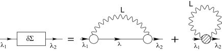
Figure 1: Fig. 1. PC corrections to the mass operator. The open circle is the vertex $g_{L}$ of the phonon creation. The gray blob denotes the phonon non-pole (“tadpole”) term.

In magic nuclei, the perturbation theory in $\delta\Sigma^{\rm PC}_{L}$ is valid [2] for solving the Dyson equation with the mass operator $\Sigma(\varepsilon){=}\Sigma_{0}{+}\delta\Sigma^{\rm PC}(\varepsilon)$. Another situation is often occurs in semi-magic nuclei [12], due to a strong mixture of some SP states with those possessing the structure of a SP state + $L$-phonon. For such cases a method is developed in [12] which is based on a direct solving the Dyson equation with the mass operator $\Sigma(\varepsilon)$. Each SP state $|\lambda\rangle$ splits to a set of $|\lambda,i\rangle$ solutions with the SP strength distribution factors $S^{i}_{\lambda}$. In [12] a method is proposed how to express the average SP energy $\varepsilon_{\lambda}$ and the average $Z_{\lambda}$ factor in terms of $\varepsilon_{\lambda}^{i}$ and $S_{\lambda}^{i}$. It is similar to the one used usually for finding the corresponding experimental values [1]. The experimental data in heavy non-magic nuclei considered in [12] are practically absent, therefore no comparison with experiment was made in that work.

Fortunately, there is a massive of data which has a direct relevance to the set of the solutions $\varepsilon_{\lambda}^{i}$ under discussion. We mean the odd-even mass differences, that is the “chemical potentials” in the notation of the theory of finite Fermi systems (TFFS) [13]:

$$\mu_{+}^{n}(Z,N)=-\left(B(Z,N+1)-B(Z,N)\right),$$ (1)

$$\mu_{-}^{n}(Z,N)=-\left(B(Z,N)-B(Z,N-1)\right).$$ (2)

$$\mu_{+}^{p}(Z,N)=-\left(B(Z+1,N)-B(Z,N)\right),$$ (3)

$$\mu_{-}^{p}(Z,N)=-\left(B(Z,N)-B(Z-1,N)\right),$$ (4)

where $B(Z,N)$ is the binding energy of the corresponding nucleus. Evidently, they are equal to one nucleon separation energies $S_{n,p}$ [14] taken with the opposite sign. For example, we have $\mu_{-}^{n}(Z,N){=}{-}S_{n}(Z,N)$ or $\mu_{+}^{n}(Z,N){=}{-}S_{n}(Z,N+1)$.

Indeed, let us write down the Lehmann spectral expansion for the Green function $G(\varepsilon;{\bf r_{1}},{\bf r_{2}})$ in the $\lambda$-representation of the functions which diagonalize $G$ [13]:

$$G_{\lambda}(\varepsilon){=}\sum_{s}\frac{|(a^{+}_{\lambda})_{s0}|^{2}}{\varepsilon{-}(E_{s}{-}E_{0}){+}i\gamma}{+}\sum_{s}\frac{|(a_{\lambda})_{s0}|^{2}}{\varepsilon{+}(E_{s}{-}E_{0}){-}i\gamma},$$ (5)

with obvious notation. The isotopic index $\tau=(n,p)$ in (5) is for brevity omitted. In both the sums, the summation is carried out for the exact states $|s\rangle$ of nuclei with one added or removed nucleon. Explicitly, if $|0\rangle$ is the ground state of the even-even ($Z,N$) nucleus, the states $|s\rangle$ in the first sum correspond to the ($Z,N+1$) one for $\tau=n$ and ($Z+1,N$) for $\tau=p$. Correspondingly, in the second sum they are ($Z,N-1$) for $\tau=n$ and (Z-1,$N$) for $\tau=p$. If $|s\rangle$ is a ground state of the corresponding odd nucleus, the corresponding pole in (5) coincides with one the chemical potentials (1) – (4). At the mean field level, they can be attributed to the SP energies $\varepsilon_{\lambda}$ with zero excitation energy, whereas with account for the PC corrections they should coincide with the corresponding energies $\varepsilon_{\lambda}^{i}$.

The calculation scheme used in [12] and in this work contains some approximations which are typical for the TFFS [13] and which are valid in heavy nuclei with accuracy of $1/A$, $A{=}N{+}Z$. At the mean field level, we relate the poles of the Green function $G(\varepsilon)$ of the even-even nucleus ($Z,N$) to the SP levels of its odd neighbors, ($Z\pm 1,N$) or ($Z,N\pm 1$). Namely, the effect of the core deformation by the odd particle or hole to the mass operator $\Sigma$ is neglected. Note that, according to the TFFS scheme, this odd particle induced deformation and the corresponding, say, quadrupole moment may be found explicitly by solving the equation for the effective field [13], which is similar to that of the quasiparticle random phase approximation (QRPA), see e.g. [15, 16]. It should be stressed that the main odd particle effect is the PC one, and we consider it explicitly. Another approximation we use at the PC stage and it concerns the characteristics of the phonons we consider. Namely, we use the QRPA solution for the $L$-phonon in the ($Z,N$) nucleus for finding the PC corrections to the SP characteristics of of these odd nuclei. Thereby, we neglect the “blocking effect” of the odd particle (hole) in the QRPA equation for $g_{L}$. Accuracy of this approximation can be estimated as $1/n_{L}$, where $n_{L}$ is the number of the particle-hole states which contribute effectively to the vertex $g_{L}$. We deal with strongly collective $2^{+}_{1}$ and $3^{-}_{1}$ states in the even lead isotopes, for which we may estimate this number as $n_{L}{\simeq}20\div 30$. A method to take into account the effect of the odd particle in the problem under consideration is developed in [17]. It is mainly important for lighter nuclei. Note also that there is a direct, in general more accurate, method to find the mass differences (1) – (4) in terms of the binding energies of each nuclei entering these relations. However, the calculation of the PC corrections to binding energies is rather cumbersome [9] and up to now there is no systematic corresponding calculations.

Let us describe briefly the method [12] to solve the PC corrected Dyson equation for the quasiparticle Green function. We should solve the following equation:

$$\left(\varepsilon-H_{0}-\delta\Sigma^{\rm PC}(\varepsilon)\right)\phi=0,$$ (6)

where $H_{0}$ is the quasiparticle Hamiltonian with the spectrum $\varepsilon_{\lambda}^{(0)}$ and wave functions $\phi_{\lambda}^{(0)}$.

In the case when several $L$-phonons are taken into account, the total PC variation of the mass operator in Eq. (6) is the sum over all phonons:

$$\delta\Sigma^{\rm PC}=\sum_{L}\delta\Sigma^{\rm PC}_{L}.$$ (7)

We deal with the normal subsystem of the semi-magic nucleus under consideration, correspondingly, $\Sigma(\varepsilon)$ is the mass operator of a normal Fermi system. In this case, the explicit expression for the pole term is well known and can be found in [2, 12]. As to the non-local term, we follow to the method developed by Khodel [8], who first considered such diagrams in the problem of PC corrections in nuclei, see also [9].

All low-lying phonons we deal with are of surface nature, the surface peak dominating in their creation amplitude:

$$g_{L}(r)=\alpha_{L}\frac{dU}{dr}+\chi_{L}(r).$$ (8)

The first term in this expression is surface peaked, whereas the in-volume addendum $\chi_{L}(r)$ is rather small. It is illustrated in Fig. 2 for the $2^{+}_{1}$ and $3^{-}_{1}$ states in ¹⁹⁸Pb. If one neglects this in-volume term $\chi_{L}$, very simple expression for the non-pole term can be obtained [9]:

$$\delta\Sigma^{\rm non-pole}_{L}=\frac{\alpha_{L}^{2}}{2}\frac{2L+1}{3}\triangle U(r).$$ (9)

Just as in [2, 12], we will below neglect the in-volume term in (8) and use Eq. (9) for the non-pole term of $\delta\Sigma_{L}^{\rm PC}$.

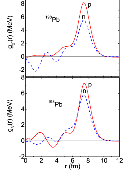
Figure 2: Fig2. (Color online) Phonon creation amplitudes $g_{L}(r)$ for two low-lying phonons in the ¹⁹⁸Pb nucleus.

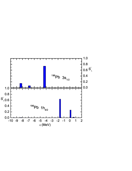
Figure 3: Fig3. (Color online) The single-particle strengh distributions ($S$-factors) of two states nearby the Fermi level for ¹⁹⁶Pb nucleus.

In this work, we consider the chain of even lead isotopes, ^180-214Pb, with account for two low-lying phonons, $2^{+}_{1}$ and $3^{-}_{1}$. Their excitation energies $\omega_{L}$ and the coefficients $\alpha_{L}$ in Eq. (8) are presented in Table 1. Comparison with existing experimental data [18] is given. We present only 3 decimal signs only of the latter to avoid a cumbersomeness of the table. On the whole, the $\omega_{L}$ values agree with the data sufficiently well. In more detail, for the interval of ^194-200Pb, the theoretical excitation energies of the $2^{+}$-states are visibly less than the experimental ones. This is a signal of the fact that our calculations overestimate the collectivity of these states and, correspondingly, the PC effect in these nuclei. The opposite situation where is for the lightest Pb isotopes, $A{<}190$, where we, evidently, underestimate the PC effect. The $\alpha_{L}$ value defines the amplitude, directly in fm, of the surface $L$-vibration in the nucleus under consideration. We see that in the most cases both the phonons we consider are strongly collective, with $\alpha_{L}{\simeq}0.3$ fm. At small values of $\omega_{L}$, the vibration amplitude behaves as $\alpha_{L}{\sim}1/\omega_{L}$ [9, 19]. Both the PC corrections to the SP energy, pole and non-pole, are proportional to $\alpha_{L}^{2}$. The ghost state $1^{-}$ is also taken into account, although the corresponding correction for nuclei under consideration is very small, see [12], because it depends on the mass number as $1/A$, $A{=}N{+}Z$.

Table 1: Table 1. Excitation energies $\omega_{L}$ (MeV) and the coefficients $\alpha_{L}$ (fm) in Eq. (8) of the $2^{+}_{1}$ and $3^{-}_{1}$ phonons in even Pb isotopes.

A	$\omega_{2}$	$\omega_{2}^{\rm exp}$	$\alpha_{2}$	$\omega_{3}$	$\omega_{3}^{\rm exp}$	$\alpha_{3}$
180	1.415	1.168(1)	0.31	2.008	–	0.35
182	1.284	0.888	0.31	1.836	–	0.35
184	1.231	0.702	0.32	1.839	–	0.36
186	1.133	0.662	0.33	1.881	–	0.34
188	1.028	0.724	0.34	1.968	–	0.34
190	0.930	0.774	0.36	2.052	–	0.33
192	0.849	0.854	0.35	2.160	–	0.32
194	0.792	0.965	0.35	2.272	–	0.32
196	0.764	1.049	0.35	2.390	2.471(?)	0.31
198	0.762	1.064	0.35	2.506	–	0.31
200	0.789	1.027	0.30	2.620	–	0.31
202	0.823	0.961	0.31	2.704	2.517	0.31
204	0.882	0.899	0.22	2.785	2.621	0.31
206	0.945	0.803	0.16	2.839	2.648	0.32
208	4.747	4.086	0.33	2.684	2.615	0.09
210	1.346	0.800	0.07	2.183	1.870(10)	0.19
				2.587	2.828(10)	0.17
212	1.444	0.805	0.17	1.788	1.820(10)	0.36
214	1.125	0.835(1)	0.19	1.469	–	0.37

Table 2: Table 2. Examples of solutions of Eq. (10) for protons in the ¹⁹⁸Pb nucleus.

$\lambda$	$i$	$\varepsilon_{\lambda}^{i}$, MeV	$S_{\lambda}^{i}$
3$s_{1/2}$	1	-8.701	0.144
	2	-7.270	0.667 $\times 10^{-1}$
	3	-4.716	0.741
	4	2.078	0.194$\times 10^{-1}$
			$\sum S_{\lambda}^{i}{=}0.970$
1$h_{9/2}$	1	-11.974	0.250 $\times 10^{-2}$
	2	-9.952	0.895 $\times 10^{-3}$
	3	-8.795	0.749 $\times 10^{-2}$
	4	-7.357	0.127 $\times 10^{-2}$
	5	-2.212	0.636
	6	-0.466	0.272
	7	0.199	0.139 $\times 10^{-1}$
	8	2.750	0.481 $\times 10^{-2}$
			$\sum S_{\lambda}^{i}{=}0.939$

Table 3: Table 3. Proton odd-even mass differences $\mu_{\pm}$ MeV for the even Pb isotopes. The mean field predictions for the Fayans EDF DF3-a and those with the PC corrections are given.

nucl.	$\lambda$	DF3-a	DF3-a + $2^{+}$	DF3-a + $(2^{+}{+}3^{-})$	exp [20]
180Pb	$\mu_{+}$, 1h9/2	3.513	3.185	3.321	—
	$\mu_{-}$, 3s1/2	-1.119	-0.571	-0.793	-0.938(0.054)
182Pb	$\mu_{+}$, 1h9/2	2.942	2.564	2.695	—
	$\mu_{-}$, 3s1/2	-1.610	-1.023	-1.268	-1.316(0.021)
184Pb	$\mu_{+}$, 1h9/2	2.360	1.906	2.093	1.527(0.094)
	$\mu_{-}$, 3s1/2	-2.104	-1.450	-1.727	-1.753(0.022)
186Pb	$\mu_{+}$, 1h9/2	1.767	1.293	1.441	1.010(0.021)
	$\mu_{-}$, 3s1/2	-2.592	-1.906	-2.152	-2.213(0.032)
188Pb	$\mu_{+}$, 1h9/2	1.172	0.683	0.806	0.461(0.031)
	$\mu_{-}$, 3s1/2	-3.072	-2.356	-2.561	-2.661(0.019)
190Pb	$\mu_{+}$, 1h9/2	0.577	0.027	0.141	-0.112(0.020)
	$\mu_{-}$, 3s1/2	-3.543	-2.750	-2.945	-3.103(0.023)
192Pb	$\mu_{+}$, 1h9/2	-0.017	-0.528	-0.420	-0.596(0.022)
	$\mu_{-}$, 3s1/2	-4.005	-3.265	-3.440	-3.572(0.020)
194Pb	$\mu_{+}$, 1h9/2	-0.608	-1.167	-1.058	-1.107(0.023)
	$\mu_{-}$, 3s1/2	-4.461	-3.673	-3.838	-4.019(0.024)
196Pb	$\mu_{+}$, 1h9/2	-1.193	-1.760	-1.658	-1.615(0.023)
	$\mu_{-}$, 3s1/2	-4.911	-4.111	-4.268	-4.494(0.025)
198Pb	$\mu_{+}$, 1h9/2	-1.769	-2.316	-2.212	-2.036(0.025)
	$\mu_{-}$, 3s1/2	-5.358	-4.569	-4.716	-4.999(0.031)
200Pb	$\mu_{+}$, 1h9/2	-2.327	-2.757	-2.648	-2.453(0.026)
	$\mu_{-}$, 3s1/2	-5.806	-5.177	-5.317	-5.480(0.039)
202Pb	$\mu_{+}$, 1h9/2	-5.806	-5.177	-5.317	-5.480(0.039)
	$\mu_{-}$, 3s1/2	-6.258	-5.612	-5.753	-6.050(0.018)
204Pb	$\mu_{+}$, 1h9/2	-3.356	-3.567	-3.447	-3.244(0.006)
	$\mu_{-}$, 3s1/2	-6.717	-6.357	-6.493	-6.637(0.003)
206Pb	$\mu_{+}$, 1h9/2	-3.818	-3.911	-3.771	-3.558(0.004)
	$\mu_{-}$, 3s1/2	-7.179	-6.976	-7.105	-7.254(0.003)
208Pb	$\mu_{+}$, 1h9/2	-4.232	-4.064	-3.959	-3.799(0.003)
	$\mu_{-}$, 3s1/2	-7.611	-7.778	-7.633	-8.004(0.007)
210Pb	$\mu_{+}$, 1h9/2	-4.670	-4.653	-4.566	-4.419(0.007)
	$\mu_{-}$, 3s1/2	-8.030	-7.971	-8.055	-8.379(0.010)
212Pb	$\mu_{+}$, 1h9/2	-5.111	-5.152	-4.980	-4.972(0.007)
	$\mu_{-}$, 3s1/2	-8.446	-8.276	-8.481	-8.758(0.044)
214Pb	$\mu_{+}$, 1h9/2	-5.555	-5.686	-5.523	-5.460(0.017)
	$\mu_{-}$, 3s1/2	-8.857	-8.620	-8.865	-9.254(0.029)
	$\langle\delta\mu\rangle_{\rm rms}$	0.385	0.321	0.218

As the non-regular PC corrections to the SP energies we examine are important only for the states nearby the Fermi surface, we limit ourselves with a model space $S_{0}$ including two shells close to it, i.e., one hole and one particle shells, and besides we retain only the negative energy states. Note that for finding the pole term $\delta\Sigma^{\rm pole}$ we use essentially wider SP space with energies $\varepsilon^{(0)}_{\lambda}{<}40$ MeV. To illustrate the method, we take for example the nucleus ¹⁹⁸Pb . The space $S_{0}$ involves 5 hole states ($1g_{7/2}$, $2d_{5/2}$, $1h_{11/2}$, $2d_{3/2}$, $3s_{1/2}$) and three particle ones ($1g_{9/2}$, $2f_{7/2}$, $1i_{13/2}$). We see that there is here only one state for each $(l,j)$ value. Therefore, we need only diagonal elements of $\delta\Sigma^{\rm PC}$ in Eq. (6). In the result, it reduces as follows:

$$\varepsilon-\varepsilon_{\lambda}^{(0)}-\delta\Sigma^{\rm PC}_{\lambda\lambda}(\varepsilon)=0.$$ (10)

Details of finding the solutions $\varepsilon_{\lambda}^{i}$ of Eq. (10) can be found in [12]. In this notation, $\lambda$ is just the index for the initial SP state from which the state $|\lambda,i\rangle$ originated. The corresponding SP strength distribution factors ($S$-factors) are:

$$S_{\lambda}^{i}=\left(1-\left(\frac{\partial}{\partial\varepsilon}\delta\Sigma^{\rm PC}(\varepsilon)\right)_{\varepsilon=\varepsilon_{\lambda}^{i}}\right)^{-1}.$$ (11)

They should obey the normalization rule:

$$\sum_{i}S_{\lambda}^{i}=1.$$ (12)

Accuracy of fulfillment of this relation is a measure of the completeness of the model space $S_{0}$ we use to solve the problem under consideration. Two examples of the sets of solutions for four $|\lambda,i\rangle$ states in ¹⁹⁸Pb are presented in Table 2. They originate from the first hole and the first particle states in the model space $S_{0}$. In this case, our prescription for the odd-even mass differences, in accordance with the Lehmann expansion (5), is as follows:

$$\mu_{+}(^{198}{\rm Pb})=-2.212\,\,{\rm MeV},$$ (13)

$$\mu_{-}(^{198}{\rm Pb})=-4.716\,\,{\rm MeV}.$$ (14)

As an illustration, we displayed in Fig. 3 the SP strength distributions ($S$-factors) of the similar two states nearby the Fermi level in the neighboring nucleus ¹⁹⁶Pb.

The similar values for all the chain under consideration are given in Table 3. In the last line, the average deviation is given of the theoretical predictions from existing experimental data:

$$\langle\delta\mu\rangle_{\rm rms}=\sqrt{\sum(\mu_{\pm}^{\rm th}-\mu_{\pm}^{\rm exp})^{2}/N_{\rm exp}},$$ (15)

where $N_{\rm exp}{=}34$. For comparison, we calculated the corresponding value for the “champion” Skyrme EDF HFB-17 [6] using the table [7] of the nuclear binding energies. It is equal to $\langle\delta\mu\rangle_{\rm rms}({\rm HFB-17}){=}0.333$ MeV. We see that accuracy of the Fayans EDF DF3-a without PC in predicting the odd-even mass differences is only a bit worse. It agrees with the original Fayans’s idea [4, 5] develop an EDF without PC corrections. However, account for the PC corrections due to two low-laying collective phonons makes agreement with the data significantly better.

To resume, a method, developed recently [12] to find the PC corrections to SP energies of semi-magic nuclei based on the direct solution of the Dyson equation with the PC corrected mass operator, is used for finding the odd-even mass difference between the even Pb isotopes and their odd-proton neighbors. The Fayans EDF DF3-a is used for generating the mean field basis. On the mean-field level, the average accuracy of the predictions for the mass differences $\langle\delta\mu\rangle_{\rm rms}({\rm DF3{-}a}){=}0.389$ MeV is only a bit worse than that (0.333 MeV) for the Skyrme EDF HFB-17 fitted to nuclear masses with highest accuracy among the self-consistent calculations. Account for the PC corrections due to the low-laying phonons $2^{+}_{1}$ and $3^{-}_{1}$ makes the agreement significantly better, $\langle\delta\mu\rangle_{\rm rms}({\rm DF3{-}a})^{\rm PC}{=}0.218$ MeV.

We acknowledge for support the Russian Science Foundation, Grants Nos. 16-12-10155 and 16-12-10161. The work was also partly supported by the RFBR Grant 16-02-00228-a. This work was carried out using computing resources of federal center for collective usage at NRC “Kurchatov Institute”, http://ckp.nrcki.ru. EES thanks the Academic Excellence Project of the NRNU MEPhI under contract by the Ministry of Education and Science of the Russian Federation No. 02. A03.21.0005.

References

- [1] H. Grawe, K. Langanke, and G. Mart nez-Pinedo, Rep. Prog. Phys. 70, 1525 (2007).
- [2] N.V. Gnezdilov, I.N. Borzov, E.E. Saperstein, and S.V. Tolokonnikov, Phys. Rev. C 89, 034304 (2014).
- [3] S.V. Tolokonnikov and E.E. Saperstein, Phys. At. Nucl. 73, 1684 (2010).
- [4] A.V. Smirnov, S.V. Tolokonnikov, S.A. Fayans, Sov. J. Nucl. Phys. 48, 995 (1988).
- [5] S.A. Fayans, S.V. Tolokonnikov, E.L. Trykov, and D. Zawischa, Nucl. Phys. A 676, 49 (2000).
- [6] S. Goriely, N. Chamel, and J. M. Pearson, Phys. Rev. Lett. 102, 152503 (2009).
-
[7]
S. Goriely, http://www-astro.ulb.ac.be/bruslib/
nucdata/ - [8] V. A. Khodel’, Sov. J. Nucl. Phys. 24, 282 (1976).
- [9] V. A. Khodel, E. E. Saperstein, Phys. Rep. 92, 183 (1982).
- [10] S. Kamerdzhiev and E. E. Saperstein, EPJA 37, 333 (2008).
- [11] S. Weinberg, Phys. Rev. Lett. 31, 494 (1973).
- [12] E.E. Saperstein, M. Baldo, S.S. Pankratov, and S.V. Tolokonnikov, JETP Lett. 104, 609 (2016).
- [13] A.B. Migdal Theory of finite Fermi systems and applications to atomic nuclei (Wiley, New York, 1967).
- [14] A. Bohr and B.R. Mottelson, Nuclear Structure (Benjamin, New York, Amsterdam, 1969.), Vol. 1.
- [15] S.V. Tolokonnikov, S. Kamerdzhiev, D. Voytenkov, S. Krewald, and E.E. Saperstein, Phys. Rev. C 84, 064324 (2011).
- [16] S.V. Tolokonnikov, S. Kamerdzhiev, S. Krewald, E.E. Saperstein, and D. Voitenkov, Eur. Phys. J. A 48, 70 (2012).
- [17] M. Baldo, P.F. Bortignon, G. Coló, D. Rizzo, and L. Sciacchitano, J. Phys. G: Nucl. Phys. 42, 085109 (2015).
- [18] S. Raman, C.W. Nestor Jr., and P. Tikkanen, At. Data Nucl. Data Tables 78, 1 (2001).
- [19] A. Bohr and B.R. Mottelson, Nuclear Structure (Benjamin, New York, 1974.), Vol. 2.
- [20] M. Wang, G. Audi, A.H. Wapstra, F.G. Kondev, M. MacCormick, X. Xu, and B. Pfeiffer, Chinese Physics C, 36, 1603 (2012).