Abstract

We introduce a new class of priors for Bayesian hypothesis testing, which we name “cake priors”. These priors circumvent Bartlett’s paradox (also called the Jeffreys-Lindley paradox); the problem associated with the use of diffuse priors leading to nonsensical statistical inferences. Cake priors allow the use of diffuse priors (having one’s cake) while achieving theoretically justified inferences (eating it too). We demonstrate this methodology for Bayesian hypotheses tests for scenarios under which the one and two sample $t$-tests, and linear models are typically derived. The resulting Bayesian test statistic takes the form of a penalized likelihood ratio test statistic. By considering the sampling distribution under the null and alternative hypotheses we show for independent identically distributed regular parametric models that Bayesian hypothesis tests using cake priors are Chernoff-consistent, i.e., achieve zero type I and II errors asymptotically. Lindley’s paradox is also discussed. We argue that a true Lindley’s paradox will only occur with small probability for large sample sizes.

Keywords: Jeffreys-Lindley-Bartlett paradoxes; improper priors; likelihood ratio tests;
Chernoff-consistent; cake priors; linear models; asymptotic properties of hypothesis tests.

1 Introduction

Determining appropriate parameter prior distributions is of paramount importance in Bayesian hypothesis testing. Bayesian hypothesis testing often centres around the concept of a Bayes factor, which was initially developed by Jeffreys (1935, 1961), and later popularized by Kass and Raftery (1995). The Bayes factor is simply the odds of the marginal likelihoods between two hypotheses and is analogous to the likelihood ratio statistic in classical statistics, where instead of maximizing the likelihoods with respect to the model parameters, the model parameters are marginalized out. In classical statistical theory testing a simple point null hypothesis against a composite alternative is routine. However, such hypothesis tests can pose severe difficulties in the Bayesian inferential paradigm where the Bayes factors may exhibit undesirable properties unless parameter prior distributions are chosen with exquisite care. This paper offers a solution to this difficulty.

Prior distributions can be chosen in an informative or uninformative fashion. Employing informative priors (either based on data from previously conducted experiments, or eliciting priors from subject matter experts) can be impractical, particularly when the number of parameters in the model is large. Furthermore, informative priors can be criticised on grounds that such priors are inherently subjective or may not let the data from the current experiment speak for itself. However, using alternative priors can also lead to problems.

One such problem occurs when using overly diffuse or flat improper priors. In the former case, as priors become more diffuse the hypothesis corresponding to the smaller model becomes increasingly favoured regardless of the evidence provided by the data. This problem occurs due to the normalizing constants of the priors dominating the expression for the Bayes factor, and is sometimes referred to as Bartlett’s paradox (e.g, Liang et al., 2008) or the Jeffreys-Lindley paradox (e.g, Robert, 1993, 2014), named after the pioneering work of Jeffreys (1935, 1961), Lindley (1957), and Bartlett (1957), whose authors identified this and other related problems associated with Bayes factors. Discussions of this paradox and the related Lindley’s paradox can be found in Aitkin (1991), Bernardo (1999), Sprenger (2013), Spanos (2013), and Robert (2014).

An extension of Bartlett’s paradox occurs in the limit where diffuse priors become flat to the point of being improper. The use of flat improper priors gives rise to arbitrary constants in the numerator and denominator of the Bayes factor (see DeGroot, 1973). Such arbitrary constants are problematic since, without suitable modification, they could be chosen by the analyst to suit any preconceived conclusions preferred, and as such, are not suitable for scientific purposes. Techniques for selecting the arbitrary constants in Bayes factors in an acceptable way when employing flat improper priors have been developed in several papers. Bernardo (1980) proposes to derive a reference prior for the null hypothesis by maximizing a measure of missing information. Spiegelhalter and Smith (1982), and Pettit (1992) use an imaginary data device leading to the arbitrary constants cancelling with other terms in the Bayes factor. A further approach to the problem of using diffuse priors was proposed by Robert (1993) who advocated for reweighing the prior odds to balance against parameter priors as prior hyperparameters become diffuse.

O’Hagan (1995) considers the problem of using flat improper priors in the calculation of the Bayes factor by splitting the data into a training and testing set. The training set is used to construct an informative prior to be used to calculate the Bayes factor using the remaining portion of the data. These ideas have been refined in O’Hagan (1997), Berger and Pericchi (1996), and Berger and Pericchi (2001). A computational drawback of some of these approaches is that the same model is fit multiple times. For models where Bayesian inferential procedures are considered too slow for fitting a single model these approaches to Bayesian testing become infeasible from a practical viewpoint.

Other Bayesian hypothesis testing approaches abandon the Bayes factor altogether by constructing hypothesis testing criterion which only enter the criterion through parameter posterior distributions themselves. These include information criteria type approaches such as the Bayesian information criterion (BIC) and the deviance information criterion (DIC). The BIC or Schwarz’s criterion uses a Laplace approximation where the prior term is assumed to be asymptotically negligible as the sample size grows (Schwarz, 1978). The DIC involves a linear combination of the log-likelihood evaluated at a suitably chosen Bayesian point estimator and the posterior expectation of the log-likelihood (Spiegelhalter et al., 2002). Under such a construction the DIC is not dominated by the prior as prior hyperparameters diverge. Similarly, posterior Bayes factors proposed by Aitkin (1991) are based on the posterior expectation of the likelihood function, rather than the joint likelihood (comprising of the model likelihood and prior). Since this only involves the prior in the calculation of the posterior distribution, the prior does not dominate posterior Bayes factors. Berger and Pericchi (1996) criticized this approach because it employs a double use of the data that is not consistent with typical Bayesian logic.

An interesting alternative approach to Bayesian hypothesis testing is that suggested in Section 6.3 of Gelman et al. (2013) who discuss examining the posterior distribution of carefully chosen test statistics such that large values of a given test statistic provides evidence against the null hypotheses. This idea is explored more formally in Gelman et al. (1996) and give rise to the concept of posterior predictive $p$-values, the probability that a test statistic of posterior predictive values is greater than the observed value of the test statistic.

Bayes factors in the context of linear model selection (Zellner and Siow, 1980; Mitchell and Beauchamp, 1988; George and McCulloch, 1993; Fernández et al., 2001; Liang et al., 2008; Maruyama and George, 2011; Bayarri et al., 2012) and generalized linear model selection (Chen and Ibrahim, 2003; Hansen and Yu, 2001; Wang and George, 2007; Chen et al., 2008; Gupta and Ibrahim, 2009; Bové and Held, 2011; Hanson et al., 2014; Li and Clyde, 2015) have received an enormous amount of attention. While we defer discussion of the types of priors used in these contexts to Section 4.3 we will draw special attention to Liang et al. (2008). Liang et al. (2008) considers several prior structures in the context of linear models. They employ Zellner’s $g$-prior (Zellner and Siow, 1980; Zellner, 1986) for the regression coefficients where $g$ is a prior hyperparameter. They consider several choices for choosing $g$ including setting $g$ to various constants, selecting $g$ using a local and global empirical Bayes procedure, and via placing a hyperprior on $g$. Their results suggest that in order for the resulting Bayes factors to be well behaved (including model selection consistent) a hyperprior needs to be placed on $g$.

In this paper we will construct a new class of priors which was inspired by the priors used in the context of linear and generalized linear models. This class of priors is constructed in such a way as to mimic Jeffreys priors (which have the desirable property that they are invariant under parameter transformations Jeffreys, 1946) in the limit as a prior hyperparameter $g$ diverges. In order to circumvent a Bartlett’s like paradox from occurring, the rate at which $g$ diverges is different in the null and alternative hypothesis in such a way that results in the cancellation of problematic terms in both the numerator and denominator of the Bayes factor.

Bayes factors using cake priors have several desirable properties. In the examples we consider the Bayes factor can be expressed as a difference in BIC values, i.e., a penalized version of the likelihood ratio test (LRT) statistic. Using properties of the LRT statistic we show that Bayesian hypothesis tests are Chernoff-consistent in the sense of (Shao, 2003, Section 2.13), i.e., they achieve asymptotically zero type I and type II errors as the sample size diverges. In contrast classical hypothesis testing procedures are usually chosen to have a fixed type I error and are consequently not Chernoff-consistent. In this respect our Bayesian hypothesis tests are superior to classical procedures whose type I error is held fixed. Due to the above properties we call the priors we develop “cake priors” since they allow the use of diffuse priors (having ones cake) while being able to perform sensible statistical inferences (eating it too). We will also discuss Lindley’s paradox in the context of cake priors and argue that generally Lindley’s paradox will only occur with vanishingly small probability for large samples.

In Section 2 we reintroduce Bayes factors, including the interpretation of Bayes factors. In Section 3 we discuss more specifically the problems associated with Bayes factors, including both Lindley’s and Bartlett’s paradoxes. In Section 4 we describe cake priors and illustrate their use in the context of one sample tests for equal means (with unknown variance), two sample tests for equal means (assuming unequal variances), linear models, and one sample tests for equal means (with known variance). In Section 5 we derive some asymptotic theory for our proposed of Bayesian hypothesis tests. In Section 6 discuss the relationship between cake priors and improper priors and discuss how arbitrary constants can be introduced into the Bayes factor. In Section 7 we take a closer look at the interpretation of Bayes factors in light of our findings. In Section 8 we conclude.

2 Bayes factors

Bayes factors are a key concept in Bayesian hypothesis testing introduced by Jeffreys (1935, 1961), although a similar concept was also developed independently by Good (1952). Suppose that we have observed the data vector ${\bf x}=(x_{1},\ldots,x_{n})^{T}$ which are observed samples from ${\mathcal{P}}=\{\,p_{i}(\,\cdot\,)\,\colon\,i=1,\ldots,n\,\}$ and we have two hypotheses $H_{0}$ and $H_{1}$ representing two models ${\mathcal{P}}_{j}=\{\,p_{ij}(\,\cdot\,|{\boldsymbol{\theta}}_{j},H_{j})\,\colon\,i=1,\ldots,n\,\}$, $j=0,1$, describing two potential distributions from which ${\bf x}$ was drawn, i.e.,

$$H_{0}\colon{\mathcal{P}}\in{\mathcal{P}}_{0}\qquad\mbox{versus}\qquad H_{1}\colon{\mathcal{P}}\in{\mathcal{P}}_{1}.$$ (1)

The models could potentially have distinct parameters from two distinct models and the models need not be nested. Let $p({\boldsymbol{\theta}}_{j}|H_{j})$ be the prior distribution under hypothesis $H_{j}$ for $j=0,1$. The Bayes factor is then defined as

$$\mbox{BF}_{01}=\frac{p({\bf x}|H_{0})}{p({\bf x}|H_{1})}=\frac{\int p({\bf x}|{\boldsymbol{\theta}}_{0},H_{0})p({\boldsymbol{\theta}}_{0}|H_{0})d{\boldsymbol{\theta}}_{0}}{\int p({\bf x}|{\boldsymbol{\theta}}_{1},H_{1})p({\boldsymbol{\theta}}_{1}|H_{1})d{\boldsymbol{\theta}}_{1}},$$

where integrals are replaced with combinatorial sums for discrete random variables. The posterior odds of $H_{0}$ to $H_{1}$ is defined by $\mbox{PO}_{01}=\mbox{BF}_{01}\times p(H_{0})/p(H_{1}),$ where the factor $p(H_{0})/p(H_{1})$ is the prior odds. Assuming $p(H_{0})=p(H_{1})=1/2$, the Bayes factors have the interpretation that when $\mbox{BF}_{01}$ is above 1 the hypothesis $H_{0}$ is favoured and when $\mbox{BF}_{01}$ is below 1 the hypothesis $H_{1}$ is favoured. However, if the prior odds is not equal to one then the posterior odds should be the focus for inference.

A Bayesian hypothesis test function $T({\bf x})\in\{0,1\}$ is based on $T({\bf x})=I(\lambda_{\mbox{\scriptsize Bayes}}>0)$ where $\lambda_{\mbox{\scriptsize Bayes}}=-2\ln\mbox{BF}_{01}$ (which we will call the Bayesian test statistic, analogous to the LRT statistic), and

$$T({\bf x})=\left\{\begin{array}[]{rl}1&\displaystyle\mbox{implies $H_{1}$ is preferred; \quad and}\\ 0&\displaystyle\mbox{implies $H_{0}$ is preferred}.\end{array}\right.$$

As indicated in the above equation, the interpretation of results based on Bayesian hypothesis tests is different from the interpretation of frequentist tests. Frequentist hypothesis testing which asks whether the data could have plausibly been drawn from the null model (based on a chosen test statistic), without reference to an alternative model (although LRT statistics are, for example, derived with reference to a specific alternative model). Furthermore, in the Bayesian paradigm preference towards a particular hypothesis is stated, rather than rejection of the null. Note that preference should not be confused with endorsement. One can have a preference between two poorly fitting models without stating that either model fits the data well.

Kass and Raftery (1995) offer an interpretation of $\lambda_{\mbox{\scriptsize Bayes}}$, and $\mbox{BF}_{10}=1/\mbox{BF}_{01}$ in Table 1 in terms of strength of evidence against the null hypothesis. In Section 7 we will take a closer look at the interpretation of Bayes factors in light of the analysis in the current paper. For the examples we consider, using the cake priors described later, the quantity $\lambda_{\mbox{\scriptsize Bayes}}$ will turn out to be a penalized version of $\lambda_{\mbox{\scriptsize LRT}}=-2[\ell_{0}(\widehat{{\boldsymbol{\theta}}}_{0})-\ell_{1}(\widehat{{\boldsymbol{\theta}}}_{1})]$ (the LRT statistic for the hypotheses in (1) where $\ell_{j}({\boldsymbol{\theta}}_{j})=\ln p({\bf x}|{\boldsymbol{\theta}}_{j},H_{j})$ and the $\widehat{{\boldsymbol{\theta}}}_{j}$’s are the MLEs under $H_{j}$) given by

$$\lambda_{\mbox{\scriptsize Bayes}}=\lambda_{\mbox{\scriptsize LRT}}-\nu\ln(n)\qquad\mbox{or}\qquad\lambda_{\mbox{\scriptsize Bayes}}=\lambda_{\mbox{\scriptsize LRT}}-\nu\ln(n)+O(n^{-1})$$ (2)

depending on the example, where $\nu$ is the difference in the number of parameters in $H_{0}$ and $H_{1}$. Intuitively one might expect $\lambda_{\mbox{\scriptsize Bayes}}$ and $\lambda_{\mbox{\scriptsize LRT}}$ to be related since the focus of both approaches are based on the ratio of likelihoods, albeit different likelihoods.

$\lambda_{\mbox{\scriptsize Bayes}}$	$\mbox{BF}_{10}$	Strength of evidence
$0$ to $2$	$1$ to $3$	not worth more than a bare mention
$2$ to $6$	$3$ to $20$	positive
$6$ to $10$	$20$ to $150$	strong
$>10$	$>150$	very strong

Table 1: Table of interpretation of Bayes factors offered by Kass and Raftery (1995).

3 Paradoxes in Bayesian hypothesis testing

Problems with Bayesian hypothesis testing based on Bayes factors, for particular combinations of hypotheses and priors, have been identified as early as 1935 by Jeffreys (1935), and later by Lindley (1957), and Bartlett (1957). As we will see for particular hypothesis tests, when parameter priors are not chosen with care, the conclusions based on Bayes factors will not be sensible. To give some context for the ensuing discussion we will now consider the hypothesis testing problem introduced by Lindley (1957) in order to illustrate potential problems.

Lindley’s example: Consider the hypothesis test where the sample is modelled via $x_{i}|\mu\sim N(\mu,\sigma^{2})$, $1\leq i\leq n$ independently, where $\mu$ and $\sigma^{2}$ are the mean and variance parameters respectively. Here $\mu$ is an unknown value to be estimated and $\sigma^{2}$ is a fixed known constant. Suppose that we wish to perform the hypothesis test

$$H_{0}\colon\mu=\mu_{0}\qquad\mbox{versus}\qquad H_{1}\colon\mu\neq\mu_{0},$$ (3)

where $\mu_{0}$ is a known constant. Under $H_{0}$ the values of all model parameters are fixed (so that under $H_{0}$ the model has zero unknown parameters), i.e., $H_{0}$ is a simple point null hypothesis. Suppose that for $H_{1}$ we employ the prior $\mu|H_{1}\sim N(\mu_{0},\tau^{2})$ where the prior variance $\tau^{2}$ is a known constant. The Bayes factor with the stated prior on $\mu$ is

$$\mbox{BF}_{01}=\sqrt{1+\frac{n\tau^{2}}{\sigma^{2}}}\exp\left[-\frac{nz({\bf x})^{2}}{2(n+\sigma^{2}/\tau^{2})}\right],$$ (4)

where $z({\bf x})=\sqrt{n}(\overline{x}-\mu_{0})/\sigma$ is the standard $z$-test statistic (see Bernardo, 1999). The $p$-value for this test is ${\mathbb{P}}(\chi_{1}^{2}>z({\bf x})^{2})$.

$\square$

If we were to choose $\mu|H_{1}$ as above then Lindley (1957) identified the following problem.

• Problem I: For any fixed $p$-value as $n\to\infty$ we have $\mbox{BF}_{01}\to\infty$.

Suppose that the observed value of $z({\bf x})$ is large so that, for any reasonably chosen level $\alpha$, the typical frequentist approach would reject the null hypothesis. For this value of $z({\bf x})$ a Bayesian procedure based on the above Bayes factor would prefer the null hypothesis for a sufficiently large $n$, drawing a contradiction between the two inferential paradigms. Problem I is associated with Lindley’s paradox, also referred to as the Lindley-Bartlett and the Jeffreys-Lindey paradox). For discussion of this see Smith and Spiegelhalter (1980); Aitkin (1991); Bernardo (1999); Sprenger (2013); Robert (2014).

We now consider a second example posed by Sprenger (2013).

Sprenger’s example: Jahn et al. (1987) used electronic and quantum-mechanical random event generators with visual feedback; the subject with alleged psychokinetic ability tries to “influence” the generator. The number of “successes” was $s=52,263,470$ and the number of trials was $n=104,490,000$. Assuming independence of each trial we have $x_{i}|\rho\sim\mbox{Bernoulli}(\rho)$, $1\leq i\leq n$ with $p\in[0,1]$. If we test

$$H_{0}\colon\rho=0.5\qquad\mbox{versus}\qquad H_{1}\colon\rho\neq 0.5,$$ (5)

a rejection of $H_{0}$ leads to evidence that the subject has psychokinetic ability. Using the data a classical hypothesis testing approach leads to a $p$-value approximately equal to $0.0003$, leading to a rejection of the null hypothesis for the $\alpha=0.05$ cut-off. A 95% confidence interval for $\rho$ is $(0.50008,0.50027)$. A standard Bayesian hypothesis test uses the prior $\rho\sim\mbox{Beta}(1/2,1/2)$ (the Jeffreys prior) leads to:

$$\lambda_{\mbox{\scriptsize Bayes}}=2\ln\mbox{Beta}(1/2+s,1/2+n-s)-2\ln(\pi)+2n\ln(2),$$ (6)

where $s=\sum_{i=1}^{n}x_{i}$. For the Bayesian test $\lambda_{\mbox{\scriptsize Bayes}}\approx-5.86$, which implies the null model is preferred and an apparent contradiction between inferential paradigms.

3.1 Resolving Lindley’s paradox

We will now resolve Lindley’s paradox in both of the above examples.

Resolving Lindley’s example: We argue that Problem I for Lindley’s example only occurs because it is assumed that the $p$-value is held fixed, and that a true Lindley’s paradox only occurs with vanishingly small probability as $n\to\infty$. The $p$-value cannot be held fixed as $n\to\infty$ as its behaviour depends on the data generation process. Let ${\bf X}=(X_{1},\ldots,X_{n})^{T}$ be a random sample. Consider the value of $\lambda_{\mbox{\scriptsize Bayes}}$ for Lindley’s example as a function of this random sample, i.e., where

$$\lambda_{\mbox{\scriptsize Bayes}}({\bf X})=\frac{nz({\bf X})^{2}}{n+\sigma^{2}/\tau^{2}}-\ln\left(1+\frac{n\tau^{2}}{\sigma^{2}}\right).$$ (7)

The first term on the right-hand side of (7) depends on the data generating process for ${\bf X}$, whereas the second term is $O(\ln(n))$. Consider the two cases:

1. If $X_{i}\stackrel{{\scriptstyle\mbox{\scriptsize iid}}}{{\sim}}N(\mu_{0},\sigma^{2})$, i.e., the data is generated from $H_{0}$. Then $z({\bf X})^{2}\sim\chi_{1}^{2}=O_{p}(1)$ and the $O(\ln(n))$ term dominates. Hence, as $n\to\infty$ we have $\lambda_{\mbox{\scriptsize Bayes}}({\bf X})\to-\infty$ implying ${\mathbb{P}}(T({\bf X})=0)\to 1$, i.e., the null hypothesis is preferred.

2. If $X_{i}\stackrel{{\scriptstyle\mbox{\scriptsize iid}}}{{\sim}}N(\mu_{1},\sigma^{2})$ for some $\mu_{1}$ with $\mu_{1}\neq\mu_{0}$, i.e., the data is generated from $H_{1}$. Then $z({\bf X})^{2}\sim\chi_{1}^{\prime 2}(n(\mu_{1}-\mu_{0})^{2}/\sigma^{2})$ where $\chi_{\nu}^{\prime 2}(\lambda)$ is the non-central chi-squared distribution with degrees of freedom $\nu$ and non-centrality parameter $\lambda$. Then $z({\bf X})^{2}=O_{p}(n)$ dominating $O(\ln(n))$ term. Then as $n\to\infty$ we have $\lambda_{\mbox{\scriptsize Bayes}}({\bf X})\to\infty$ implying ${\mathbb{P}}(T({\bf X})=1)\to 1$, i.e., the alternative hypothesis is preferred.

Note that 1. implies that a test based on the above Bayes factor has vanishing type I error as $n\to\infty$ and 2. implies that the Bayesian test is consistent in the sense of (Lehmann, 2004, Section 3.3). Combining 1. and 2. implies that the test is Chernoff consistent (see Section 5 for a formal definition).

Resolving Sprenger’s example: Using properties of the beta function, the gamma function, and Stirling’s approximation leads to approximating (6) by

$$\lambda_{\mbox{\scriptsize Bayes}}({\bf x})=\lambda_{\mbox{\tiny LRT}}({\bf x})-\ln(n)-\ln(\pi/2)+O(n^{-1}),$$

where $\lambda_{\mbox{\tiny LRT}}$ is the LRT statistic corresponding to the hypotheses (5). Again, Lindley’s paradox occurs here if we consider $\lambda_{\mbox{\tiny LRT}}({\bf x})$ (or equivalently the $p$-value) to be fixed. If $\lambda_{\mbox{\tiny LRT}}$ is held fixed and $n$ diverges then the null hypothesis will be preferred in the limit. Let ${\bf X}=(X_{1},\ldots,X_{n})^{T}$ be a random sample. We will later show (see Section 5) that

$$\lambda_{\mbox{\tiny LRT}}({\bf X})=\left\{\begin{array}[]{rl}O_{p}(1)&\mbox{if $H_{0}$ is true; \, and}\\ O_{p}(n)&\mbox{if $H_{1}$ is true.}\\ \end{array}\right.$$

Hence, as $n\to\infty$ we have $\lambda_{\mbox{\scriptsize Bayes}}({\bf X})\to-\infty$ if $H_{0}$ is true, and $\lambda_{\mbox{\scriptsize Bayes}}({\bf X})\to\infty$ if $H_{1}$ is true so that the test based on $\lambda_{\mbox{\scriptsize Bayes}}$ is Chernoff consistent. Figure 1 illustrates the empirical probabilities for rejecting the null hypothesis (for the frequentist test at the 5% level) or preferring the alternative hypothesis (for the Bayesian test) based on simulating $10^{6}$ datasets with the true value of $\rho$ in the set $\{0.5,0.5001,0.5002,0.5003\}$ for $n$ on a grid form $n=10^{6.5}$ to $n=10^{9}$. The vertical line in Figure 1 indicates the actual value of $n$ in Sprenger’s example and the dashed grey line illustrates the estimated empirical probability that the two tests disagree. In Figure 1 we see that when $H_{0}$ is false, as the sample size increases, both tests reject the null as $n$ or $\rho$ grows. When $\rho=0.5$ the frequentist test accepts the null model at the 5% level, while the Bayesian test prefers the null model with very low probability. Furthermore, at the actual value of $n$ in the experiment the disagreement between frequentist and Bayesian tests could have occurred by chance with relatively high probability. However, for much larger large $n$ such a disagreement will only occur with low probability when $H_{1}$ is true.

$\square$

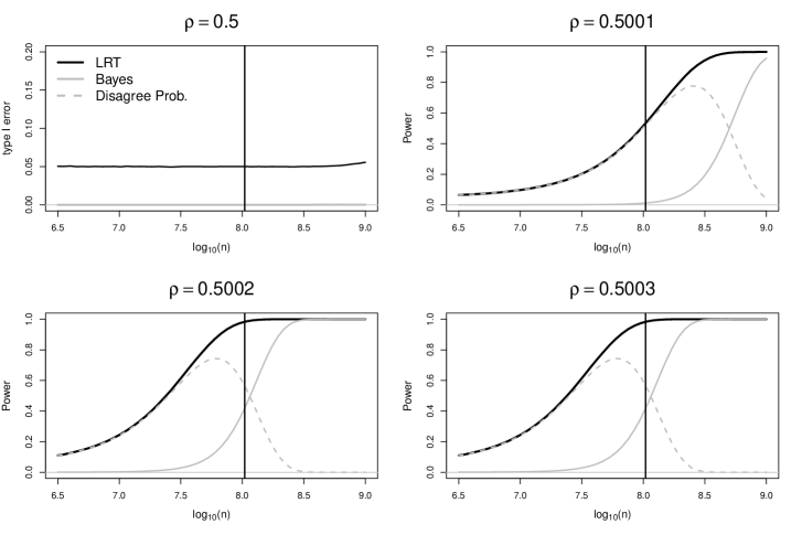
Figure 1: Empirical probabilities of rejecting the null hypothesis/preferring the alternative hypothesis for the simulation described in Section 3 comparing the LRT and Bayesian tests when $\rho_{\mbox{\scriptsize true}}\in[0.5,0.5004]$ and $n=104,490,000$.

We now note for Lindley’s example that the test based on $\lambda_{\mbox{\scriptsize Bayes}}$ is an LRT test with an extremely small level $\alpha$ given by $\alpha={\mathbb{P}}[\chi_{1}^{2}>\{1+\sigma^{2}/(n\tau^{2})\}\ln(1+n\tau^{2}/\sigma^{2})]$ (when $\tau^{2}$ is large) while for Sprenger’s example that the test based on $\lambda_{\mbox{\scriptsize Bayes}}$ is in also an LRT test with asymptotic level $\alpha={\mathbb{P}}[\chi_{1}^{2}>\ln(n)+\ln(\pi/2)]$. Hence, we note, as was also argued by Naaman (2016) and noted by Lindley (1957), that Lindley’s paradox can also be resolved by letting the level of the test $\alpha$ in the frequentist test tend to zero as $n\to\infty$. We discuss Lindley’s paradox more generally in Section 5.2.

The above expression for the level of the test for Lindley’s example draws attention to a second problem for Lindley’s example which does not occur in Sprenger’s example.

• Problem II: For any given $p$-value as $\tau^{2}\to\infty$ we have $\mbox{BF}_{01}\to\infty$.

This problem occurs because as the prior variance increases the level of the test decreases.

Problem II is referred to as Bartlett’s paradox in Liang et al. (2008) and the Jeffreys-Lindley paradox in Robert (2014). Bartlett’s paradox is paradoxical since as $\tau^{2}$ becomes large the prior on $\mu$ becomes increasingly vague regarding the location of $\mu$. However, in the attempt to be vague about the location of $\mu$ the prior becomes “informative” in favouring $H_{0}$ as the preferred hypothesis, again, regardless of the evidence provided by the data. Unlike Lindley’s paradox, we believe that Bartlett’s paradox is a real problem in practice since the use of diffuse priors can sometimes lead to testing procedures with extremely small power. Our proposed cake priors described in the next section circumvent this problem.

4 Cake priors

Consider the general hypotheses (1). Let $d_{0}$ and $d_{1}$ be the dimensions of ${\boldsymbol{\theta}}_{0}$ and ${\boldsymbol{\theta}}_{1}$ respectively. For the time being we will assume that $0<d_{0}\leq d_{1}$ (later we will consider $0\leq d_{0}\leq d_{1}$). Define the observed information and Fisher information matrices as ${\bf J}({\boldsymbol{\theta}})=-\nabla_{\boldsymbol{\theta}}^{2}\ell({\boldsymbol{\theta}})$ and ${\mathcal{I}}({\boldsymbol{\theta}})={\mathbb{E}}_{x_{i}|{\boldsymbol{\theta}}}\left[-\nabla_{\boldsymbol{\theta}}^{2}\ln p(x_{i}|{\boldsymbol{\theta}})\right]$ respectively. Define the mean observed information matrix as $\widetilde{{\bf J}}({\boldsymbol{\theta}})=n^{-1}{\bf J}({\boldsymbol{\theta}})$ and the mean expected observed information matrix as $\widetilde{{\mathcal{I}}}({\boldsymbol{\theta}})=n^{-1}{\mathbb{E}}_{{\bf x}|{\boldsymbol{\theta}}}\left[{\bf J}({\boldsymbol{\theta}})\right]$. We will denote the Fisher information matrix under the null and alternative hypotheses as ${\mathcal{I}}_{0}({\boldsymbol{\theta}}_{0})$ and ${\mathcal{I}}_{1}({\boldsymbol{\theta}}_{1})$ with similar use of subscripts to denote similar quantities such as ${\bf J}$, $\widetilde{{\mathcal{I}}}$ and $\widetilde{{\bf J}}$. We define a Jeffreys prior as any density for ${\boldsymbol{\theta}}$ such that $p({\boldsymbol{\theta}})\propto|{\mathcal{I}}({\boldsymbol{\theta}})|^{1/2}$.

We construct cake priors using the following ingredients:

1. Define the priors

   $$p({\boldsymbol{\theta}}_{j}|H_{j};g_{j})=\exp\left[-\tfrac{d_{j}}{2}\ln(2\pi g_{j})+\tfrac{1}{2}\ln|{\bf P}_{j}({\boldsymbol{\theta}}_{j})|-\tfrac{1}{2g_{j}}{\boldsymbol{\theta}}_{j}^{T}{\bf P}_{j}({\boldsymbol{\theta}}_{j}){\boldsymbol{\theta}}_{j}\right],$$ (8)

   where ${\bf P}_{j}({\boldsymbol{\theta}}_{j})$ is a prior precision matrix (assumed to be full rank). For all of the examples considered in this paper we will use ${\bf P}_{j}({\boldsymbol{\theta}}_{j})=\widetilde{{\mathcal{I}}}_{j}({\boldsymbol{\theta}}_{j})$.

2. Set $g_{j}=h^{1/d_{j}}$ where $h$ is a common hyperparameter.

3. Calculate the Bayes Factor as

   $$\mbox{BF}_{01}(h)=\left[\displaystyle\int p({\bf x}|{\boldsymbol{\theta}}_{0},H_{0})p({\boldsymbol{\theta}}_{0}|H_{0};h^{1/d_{0}})d{\boldsymbol{\theta}}_{0}\right]\Big{/}\left[\displaystyle\int p({\bf x}|{\boldsymbol{\theta}}_{1},H_{1})p({\boldsymbol{\theta}}_{1}|H_{1};h^{1/d_{1}})d{\boldsymbol{\theta}}_{1}\right].$$

4. Optional: Let $h\to\infty$ if flat priors are desired.

When ${\bf P}_{j}({\boldsymbol{\theta}}_{j})\propto{\mathcal{I}}_{j}({\boldsymbol{\theta}}_{j})$, $j=0,1$, (8) leads to a Bayes Factor, in the limit as $g_{j}\to\infty$, that would have been obtained if a Jeffrey’s prior is used. When ${\bf P}_{j}({\boldsymbol{\theta}}_{j})\propto{\mathcal{I}}_{j}({\boldsymbol{\theta}}_{j})$, $j=0,1$, (8) are Jeffreys priors in the limit as $g_{j}\to\infty$. Letting $g_{j}\to\infty$ would be problematic if not for 2. which leads to certain terms involving $h$ cancelling in the Bayes factor. As $h\to\infty$, the priors on ${\boldsymbol{\theta}}_{j}$ are made diffuse, but at a rate that depends on the $d_{j}$’s. We keep 4. optional due to the fact that particular Bayesian procedures may require proper priors. For particular examples in the coming subsections the above steps will raise complications. These include: (A) Model parameters may not be defined on the whole real line, e.g., variances. Priors of the form (8) are not appropriate for such model parameters; (B) The priors $p({\boldsymbol{\theta}}_{j}|g_{j},H_{j})$ may not be proper densities; and (C) If $d_{0}=0$ using $g=h^{1/d_{j}}$ is problematic. The examples in the subsections below will illustrate how each of these complications can be handled. (A) & (B) will be dealt with in sections 4.1 and 4.2. Complication (C) will be dealt with in Section 4.4.

We will now give some intuition for how cake priors avoid Bartlett’s paradox via the following heuristic argument. Let ${\bf P}_{j}({\boldsymbol{\theta}}_{j})\equiv{\bf P}_{j}$, i.e., the prior precision matrices are constant, then letting $\mbox{BF}_{01}=\left[\int p({\bf x}|{\boldsymbol{\theta}}_{0},H_{0})p({\boldsymbol{\theta}}_{0}|H_{0};g_{0})d{\boldsymbol{\theta}}_{0}\right]/\left[\int p({\bf x}|{\boldsymbol{\theta}}_{1},H_{1})p({\boldsymbol{\theta}}_{1}|H_{1};g_{1})d{\boldsymbol{\theta}}_{1}\right],$ (which depends on $g_{0}$ and $g_{1}$ rather than $h$). Then the Bayesian test statistic is

$$\begin{array}[]{l}\displaystyle\lambda_{\mbox{\scriptsize Bayes}}\\ \quad=2\ln\left[\frac{\displaystyle\int\exp\left\{\ell_{1}({\boldsymbol{\theta}}_{1})-\tfrac{{\boldsymbol{\theta}}_{1}^{T}{\bf P}_{1}{\boldsymbol{\theta}}_{1}}{2g_{1}}\right\}d{\boldsymbol{\theta}}_{1}}{\displaystyle\int\exp\left\{\ell_{0}({\boldsymbol{\theta}}_{0})-\tfrac{{\boldsymbol{\theta}}_{0}^{T}{\bf P}_{0}{\boldsymbol{\theta}}_{0}}{2g_{0}}\right\}d{\boldsymbol{\theta}}_{0}}\right]+d_{0}\ln(2\pi g_{0})-d_{1}\ln(2\pi g_{1})+\ln(|{\bf P}_{1}|/|{\bf P}_{0}|)\\[17.22217pt] \quad\displaystyle=2\ln\left[\frac{\int p({\bf x}|{\boldsymbol{\theta}}_{1},H_{1})d{\boldsymbol{\theta}}_{1}}{\int p({\bf x}|{\boldsymbol{\theta}}_{0},H_{0})d{\boldsymbol{\theta}}_{0}}\right]+d_{0}\ln(2\pi g_{0})-d_{1}\ln(2\pi g_{1})+\ln(|{\bf P}_{1}|/|{\bf P}_{0}|)+O(g_{0}^{-1}+g_{1}^{-1})\end{array}$$

where the second line is obtained using a Taylor series argument in $g_{0}$ and $g_{1}$. Ignoring the dependency of $O(g_{j}^{-1})$ terms on the ${\boldsymbol{\theta}}_{j}$’s, using Laplace’s method on the numerator and denominator of the first term in the second line above, and setting ${\bf P}_{j}=\widetilde{{\bf J}}_{j}(\widehat{{\boldsymbol{\theta}}}_{j})$ (where $\widehat{{\boldsymbol{\theta}}}_{j}$ are the MLEs for the ${\boldsymbol{\theta}}_{j}$’s), leads to

$$\begin{array}[]{rl}\displaystyle\lambda_{\mbox{\scriptsize Bayes}}&\displaystyle=\lambda_{\mbox{\scriptsize LRT}}-\nu\ln(n)+d_{0}\ln(g_{0})-d_{1}\ln(g_{1})+O(g_{0}^{-1}+g_{1}^{-1}+n^{-1}).\end{array}$$ (9)

The $O(n^{-1})$ error follows from the relative error of the Laplace’s method applied to the numerator and denominator (Tierney et al., 1989; Kass et al., 1990). Suppose that $g_{0}=g_{1}=g$. Then using the asymptotic $\chi_{\nu}^{2}$ distribution $\lambda_{\mbox{\scriptsize LRT}}$ the level of the test using (9) is $\alpha={\mathbb{P}}[\chi_{\nu}^{2}\geq\nu\ln(ng)].$ So that again we see that the power of the test goes to 0 as $g\to\infty$. Here also we see that setting $g_{0}$ to be a large constant (making the prior for ${\boldsymbol{\theta}}_{0}$ diffuse) leads the test to preferring $H_{0}$ while making $g_{1}$ large leads to preferring $H_{1}$. Hence, the relative rates that $g_{0}$ and $g_{1}$ diverge must be considered.

Setting $g_{j}=h^{1/d_{j}}$ means that $d_{0}\ln(g_{0})=d_{1}\ln(g_{1})$ and leads to $\lambda_{\mbox{\scriptsize Bayes}}=\lambda_{\mbox{\scriptsize LRT}}-\nu\ln(n)+O(h^{-1/d_{0}}+h^{-1/d_{1}}+n^{-1})$. For sufficiently large $h$ and $n$ we have $\lambda_{\mbox{\scriptsize Bayes}}\approx\lambda_{\mbox{\scriptsize LRT}}-\nu\ln(n)$. The level of the test becomes approximately $\alpha={\mathbb{P}}[\chi_{\nu}^{2}\geq\nu\ln(n)]$. We recognise the above arguments are informal in nature and will shortly illustrate cake priors in concrete examples.

Lastly, well us briefly discuss the choice of ${\bf P}_{j}$. Setting ${\bf P}_{j}={\bf I}$ leads to $\lambda_{\mbox{\scriptsize Bayes}}=\lambda_{\mbox{\scriptsize LRT}}-\nu\ln(n)+\ln|\widetilde{{\bf J}}_{0}(\widehat{{\boldsymbol{\theta}}}_{0})|-\ln|\widetilde{{\bf J}}_{1}(\widehat{{\boldsymbol{\theta}}}_{1})|+O(h^{-1/d_{0}}+h^{-1/d_{1}}+n^{-1}).$ This would be undesirable because of the additional computational burden of the log-determinant terms (which can be considerable in some contexts), and because if $\lambda_{\mbox{\scriptsize LRT}}\approx\nu\ln(n)$ we would prefer the model with larger $\ln|\widetilde{{\bf J}}_{j}(\widehat{{\boldsymbol{\theta}}}_{j})|$, i.e., larger standard errors. For this reason we would like ${\bf P}_{j}\approx\widetilde{{\bf J}}_{j}(\widehat{{\boldsymbol{\theta}}}_{j})$ so that at least approximate cancellation occurs.

4.1 One sample test for equal means (with unknown variance)

Consider the hypothesis test (3) where $x_{i}|\mu,\sigma^{2}\stackrel{{\scriptstyle\mbox{\scriptsize iid}}}{{\sim}}N(\mu,\sigma^{2})$, $1\leq i\leq n$, where $\mu$ and $\sigma^{2}$ are the mean and variance parameters respectively. Suppose now that both $\mu$ and $\sigma^{2}$ are unknown parameters to be estimated (unlike the example in Section 2 where $\sigma^{2}$ was assumed to be known).

The mean expected information matrices for the null and alternative hypothesis respectively are

$$\widetilde{{\mathcal{I}}}_{0}(\sigma^{2})=1/(2\sigma^{4})\qquad\mbox{and}\qquad\widetilde{{\mathcal{I}}}_{1}(\mu,\sigma^{2})=\left[\begin{array}[]{cc}\sigma^{-2}&0\\ 0&1/(2\sigma^{4})\end{array}\right],$$

which coincide with the Fisher information matrices in this case. Hence, Jeffreys priors for $\mu$ and $\sigma^{2}$ are $p(\mu)\propto 1$ and $p(\sigma^{2})\propto(\sigma^{2})^{-1}I(\sigma^{2}>0)$ respectively.

We cannot directly use the methodology outlined in Section 4 as $\sigma^{2}>0$. To handle this complication we use the transformation $\sigma^{2}=\exp(s)$. Under this transformation the mean expected information matrices become: $\widetilde{{\mathcal{I}}}_{0}(s)=1/2$ and $\widetilde{{\mathcal{I}}}_{1}(\mu,s)=\mbox{diag}(\exp(-s),1/2)$. Using the steps for Section 4 under this transformation we have $s|H_{0}\sim N(0,2g_{0})$, i.e., $p(s|H_{0})=[2\pi(2g_{0})]^{-1/2}\exp[-s^{2}/(4g_{0})]$. Transforming back to the $\sigma^{2}$ parametrisation gives $\sigma^{2}|H_{0}\sim LN(0,2g_{0}),$ with density which is a Jeffreys prior for $\sigma^{2}$ in the limit as $g_{0}\to\infty$.

Note that for $H_{1}$ the upper left entry of $\widetilde{{\mathcal{I}}}_{1}(\mu,s)$ depends on $s$. This implies a conditional dependence of $\mu$ on $s$ which leads to $\mu|s,H_{1}\sim N(0,g_{1}\exp(s))$ and $s|H_{1}\sim N(0,2g_{1})$. Transforming back from the parametrisation in $s$ to the parametrisation using $\sigma^{2}$ gives $\mu|\sigma^{2},H_{1}\sim N(0,g_{1}\sigma^{2})$ and $\sigma^{2}|H_{1}\sim LN(0,2g_{1}).$ Note again that these are both Jeffreys priors in the limit as $g_{1}\to\infty$.

The marginal distributions of ${\bf x}$ given $H_{0}$ and $H_{1}$ are

$$\begin{array}[]{ll}\displaystyle p({\bf x}|H_{0})=\int_{0}^{\infty}\frac{1}{\sqrt{2\pi}^{n}}\exp\left[-\tfrac{n+2}{2}\ln(\sigma^{2})-\tfrac{n\widehat{\sigma}_{0}^{2}}{2\sigma^{2}}-\tfrac{\ln(4\pi g_{0})}{2}-\tfrac{(\ln\sigma^{2})^{2}}{4g_{0}}\right]d\sigma^{2},\qquad\mbox{and}\\[8.61108pt] \displaystyle p({\bf x}|H_{1})=\int_{0}^{\infty}\frac{1}{\sqrt{2\pi}^{n}}\exp\left[-\tfrac{n+2}{2}\ln(\sigma^{2})-\tfrac{n\widehat{\sigma}_{g}^{2}}{2\sigma^{2}}-\tfrac{\ln(4\pi g_{1}^{2})}{2}-\tfrac{(\ln\sigma^{2})^{2}}{4g_{1}}-\tfrac{1}{2}\ln\left(n+\tfrac{1}{g_{1}}\right)\right]d\sigma^{2},\end{array}$$

where $\widehat{\sigma}_{0}^{2}=n^{-1}\|{\bf x}-\mu_{0}{\bf 1}\|^{2}$, and $\widehat{\sigma}_{g}^{2}=n^{-1}[\|{\bf x}\|^{2}-(n\overline{x})^{2}/(n+g^{-1})]$. Suppose that we were to use $g=g_{0}=g_{1}$ and let $g\to\infty$. Then we would see a manifestation of Bartlett’s paradox where the null hypothesis is favoured since $\mbox{BF}_{01}\to\infty$ as $g\to\infty$. If we instead use $g_{0}=h$ and $g_{1}=h^{1/2}$ then the Bayes factor simplifies to

$$\begin{array}[]{rl}\mbox{BF}_{01}(h)=&\displaystyle\frac{\displaystyle\int_{0}^{\infty}\exp\left[-\left(\tfrac{n}{2}+1\right)\ln(\sigma^{2})-\frac{n\widehat{\sigma}_{0}^{2}}{2\sigma^{2}}-\frac{(\ln\sigma^{2})^{2}}{4h}\right]d\sigma^{2}}{\displaystyle\int_{0}^{\infty}\exp\left[-\left(\tfrac{n}{2}+1\right)\ln(\sigma^{2})-\frac{n\widehat{\sigma}_{h^{1/2}}^{2}}{2\sigma^{2}}-\frac{(\ln\sigma^{2})^{2}}{4h^{1/2}}-\tfrac{1}{2}\ln(n+h^{-1/2})\right]d\sigma^{2}}\end{array}$$

which can be evaluated using univariate quadrature or other methods for any fixed $h>0$.

Since both the above integrands are monotonic as a function of $h$ with a well defined limit as $h\to\infty$ we can apply the monotonic convergence theorem and take the limit $h\to\infty$ inside both integrals. After simplifications including $\widehat{\sigma}_{h}^{2}\to\widehat{\sigma}_{1}^{2}$ where $\widehat{\sigma}_{1}^{2}=n^{-1}\|{\bf x}-\overline{x}{\bf 1}\|^{2}$ is the MLE for $\sigma^{2}$ under the alternative hypothesis we obtain $\lambda_{\mbox{\scriptsize Bayes}}=\lambda_{\mbox{\scriptsize LRT}}-\ln(n),$ where $\lambda_{\mbox{\scriptsize LRT}}=n\ln(\widehat{\sigma}_{0}^{2})-n\ln(\widehat{\sigma}_{1}^{2})$ is the LRT statistic corresponding to the hypothesis (3).

As $h\to\infty$ the parameter posterior distributions are given by

$$\sigma^{2}|{\bf x},H_{0}\sim\mbox{IG}\left(\tfrac{n}{2},\tfrac{n}{2}\widehat{\sigma}_{0}^{2}\right),\quad\mu|{\bf x},H_{1}\sim t_{n}(\overline{x},n^{-1}\widehat{\sigma}_{1}^{2}),\quad\mbox{and}\quad\sigma^{2}|{\bf x},H_{1}\sim\mbox{IG}\left(\tfrac{n}{2},\tfrac{n}{2}\widehat{\sigma}_{1}^{2}\right).$$

As a computational short-cut if the integrand is a monotonic function of $h$ with a well defined limit as $h\to\infty$ we will write

$$\begin{array}[]{l}\displaystyle p({\bf x}|H_{0})\displaystyle\stackrel{{\scriptstyle h\Rightarrow\infty}}{{=}}\int_{0}^{\infty}\exp\left[-\left(\tfrac{n}{2}+1\right)\ln(\sigma^{2})-\tfrac{n\widehat{\sigma}_{0}^{2}}{2\sigma^{2}}\right]d\sigma^{2},\qquad\mbox{and}\\[4.30554pt] \displaystyle p({\bf x}|H_{1})\displaystyle\stackrel{{\scriptstyle h\Rightarrow\infty}}{{=}}\int_{0}^{\infty}\exp\left[-\left(\tfrac{n}{2}+1\right)\ln(\sigma^{2})-\tfrac{n\widehat{\sigma}_{1}^{2}}{2\sigma^{2}}-\tfrac{1}{2}\ln(n)\right]d\sigma^{2},\end{array}$$

where the notation $\stackrel{{\scriptstyle h\Rightarrow\infty}}{{=}}$ is used to denote “equality in the limit as $h\rightarrow\infty$ after terms related to $h$ cancel in the numerator and denominator in the Bayes factor, or terms related to $h$ vanish as $h$ diverges in the Bayes factor.” The above expressions can be more easily simplified using standard results to reach the same expression for $\lambda_{\mbox{\scriptsize Bayes}}$ as above.

We conduct the following short simulation study to illustrate the differences between the LRT and the Bayesian test for this problem. Letting $\mu_{0}=0$ we simulate a single set of data from $x_{i}\sim N(\mu_{\mbox{\scriptsize true}},1)$, $1\leq i\leq n$. After simulating $10^{6}$ such datasets for all values of $\mu_{\mbox{\scriptsize true}}$ in the set $\{0,0.05,0.25,0.5\}$ and a grid of $n$ from $n=15$ to $n=1000$ we plot in Figure 2 the empirical probabilities of rejecting the null hypothesis (for the LRT test) using $\alpha=0.05$ or preferring the alternative hypothesis (for the Bayesian test).

From Figure 2 we see empirically that the type I error of the Bayesian test is tending to 0 as $n$ grows when $H_{0}$ is true, whereas the LRT test has, by design, a type I error of $0.05$. When $H_{1}$ is true and $\ln(n)<\chi^{2}_{1,\alpha}$ the Bayesian test is more powerful than the LRT test, and when $H_{1}$ is true and $\ln(n)>\chi^{2}_{1,\alpha}$ the LRT test is more powerful than the Bayesian test. When $\mu_{\mbox{\scriptsize true}}\in\{0.25,0.5\}$ both tests appear to have power tending to 1 as $n$ grows. Lastly, for the case $\mu_{\mbox{\scriptsize true}}=0.5$ when $\ln(n)>\chi^{2}_{1,\alpha}$ both have very similar power.

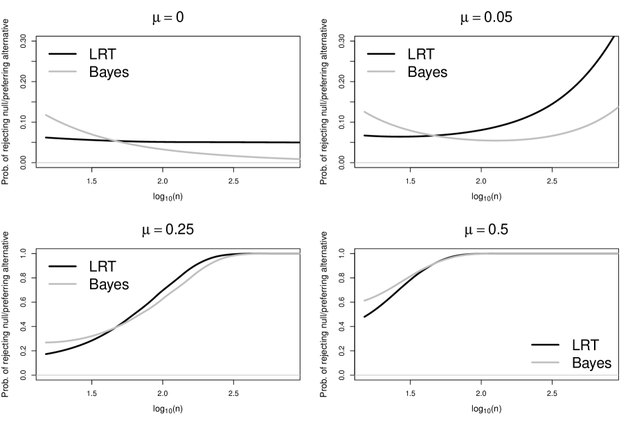
Figure 2: Empirical probabilities of rejecting the null hypothesis/preferring the alternative hypothesis for the simulation described in Section 4.1 comparing the LRT and Bayesian tests when $\mu_{\mbox{\scriptsize true}}\in\{0,0.05,0.25,0.5\}$.

4.2 Two sample test for equal means

Suppose we have data ${\bf x}=(x_{1},\ldots,x_{n})^{T}$. We want to test whether the first $n_{0}$ samples ${\bf x}_{0}=(x_{1},\ldots,x_{n_{0}})^{T}$ from class 0 come from the same normal population as the second $n_{1}$ samples ${\bf x}_{1}=(x_{n_{0}+1},\ldots,x_{n})^{T}$ from class 1 with $n_{0}+n_{1}=n$. We wish to test

$$\begin{array}[]{l}H_{0}\colon x_{i}|\mu,\sigma^{2}\sim N(\mu,\sigma^{2}),\ 1\leq i\leq n,\qquad\mbox{versus}\\ H_{1}\colon\left\{\begin{array}[]{l}x_{i}|\mu_{0},\sigma_{0}^{2}\sim N(\mu_{0},\sigma_{0}^{2}),\ 1\leq i\leq n_{0},\\[4.30554pt] x_{i}|\mu_{1},\sigma_{1}^{2}\sim N(\mu_{1},\sigma_{1}^{2}),\ n_{0}+1\leq i\leq n,\end{array}\right.\end{array}$$ (10)

where $\mu$, $\sigma^{2}$, $\mu_{0}$, $\sigma_{0}^{2}$, $\mu_{1}$ and $\sigma_{1}^{2}$ are the means and variances under the one and two group hypotheses respectively. Here ${\boldsymbol{\theta}}_{0}=(\mu,\sigma^{2})^{T}$ with $d_{0}=2$ and ${\boldsymbol{\theta}}_{1}=(\mu_{0},\mu_{1},\sigma_{0}^{2},\sigma_{1}^{2})^{T}$ with $d_{1}=4$. Using similar arguments as in Section 4.1 with ${\bf P}_{0}({\boldsymbol{\theta}}_{0})=\widetilde{{\mathcal{I}}}_{0}({\boldsymbol{\theta}}_{0})=\mbox{diag}[\sigma^{-2},1/(2\sigma^{4})]$ and ${\bf P}_{1}({\boldsymbol{\theta}}_{1})=\widetilde{{\mathcal{I}}}_{1}({\boldsymbol{\theta}}_{1})=\mbox{diag}[n_{0}/(n\sigma_{0}^{2}),n_{1}/(n\sigma_{1}^{2}),n_{0}/(2n\sigma_{0}^{4}),n_{1}/(2n\sigma_{1}^{4})]$ leads to the priors

$$\begin{array}[]{c}\mu|\sigma^{2},H_{0}\sim N(0,g_{0}\sigma^{2}),\qquad\sigma^{2}|H_{0}\sim LN(0,2g_{0}),\\[4.30554pt] \mu_{0}|\sigma_{1}^{2},H_{1}\sim N(0,g_{1}(n/n_{0})\sigma_{0}^{2}),\qquad\mu_{1}|\sigma_{1}^{2},H_{1}\sim N(0,g_{1}(n/n_{1})\sigma_{1}^{2}),\\[4.30554pt] \sigma_{0}^{2}|H_{1}\sim LN(0,2(n/n_{0})g_{1}),\quad\mbox{and}\quad\sigma_{1}^{2}|H_{1}\sim LN(0,2(n/n_{1})g_{1}).\end{array}$$

Setting $g_{j}=h^{1/d_{j}}$, $j=0,1$ results in

$$\begin{array}[]{l}\displaystyle p({\bf x}|H_{0})\\ \begin{array}[]{cl}\ =&\displaystyle\int_{0}^{\infty}\frac{1}{\sqrt{2\pi}^{n}}\exp\left[-\tfrac{n+2}{2}\ln(\sigma^{2})-\tfrac{n\widehat{\sigma}_{h^{1/2}}^{2}}{2\sigma^{2}}-\tfrac{\ln(4\pi h)}{2}-\tfrac{(\ln\sigma^{2})^{2}}{4h}-\tfrac{1}{2}\ln\left(n+\tfrac{1}{\sqrt{h}}\right)\right]d\sigma^{2}\\[8.61108pt] \ \stackrel{{\scriptstyle h\Rightarrow\infty}}{{=}}&\displaystyle\int_{0}^{\infty}\frac{1}{\sqrt{2\pi}^{n}}\exp\left[-\tfrac{n+2}{2}\ln(\sigma^{2})-\tfrac{n\widehat{\sigma}^{2}}{2\sigma^{2}}-\tfrac{\ln(4\pi)}{2}-\tfrac{1}{2}\ln(n)\right]d\sigma^{2}\\[8.61108pt] \ =&\displaystyle\exp\left[\ln p({\bf x}|\widehat{{\boldsymbol{\theta}}}_{0})+\xi\left(\tfrac{n}{2}\right)-\tfrac{1}{2}\ln(2)-\tfrac{1}{2}\ln(n)\right],\end{array}\end{array}$$

where $\xi(x)=\ln\Gamma(x)+x-x\ln(x)-(1/2)\ln(2\pi)$ and $\ln p({\bf x}|\widehat{{\boldsymbol{\theta}}}_{0})=-(n/2)\ln\left(2\pi\widehat{\sigma}^{2}\right)-n/2$ is the log-likelihood of the null model evaluated at its MLE $\widehat{{\boldsymbol{\theta}}}_{0}$. Similarly, $p({\bf x}_{0}|H_{1},h)$ is

$$\begin{array}[]{rcl}\displaystyle p({\bf x}_{0}|H_{1})\par&=&\displaystyle\int_{0}^{\infty}\tfrac{1}{\sqrt{2\pi}^{n_{0}}}\exp\Big{[}-\left(\tfrac{n_{0}}{2}+1\right)\ln(\sigma_{0}^{2})-\tfrac{1}{2\sigma_{0}^{2}}\left\{\|{\bf x}_{0}\|^{2}-\tfrac{(n_{0}\overline{x}_{0})^{2}}{n_{0}+(n_{0}/n)h^{-1/4}}\right\}\\ &&\displaystyle\qquad-\tfrac{1}{2}\ln(n+h^{-1/4})-\tfrac{1}{2}\ln(2\pi(2n/n_{0})h^{1/2})-\tfrac{(\ln\sigma_{0}^{2})^{2}}{4(n/n_{0})h^{1/4}}\Big{]}d\sigma_{0}^{2}.\par\par\par\end{array}$$

By construction the $\ln(h^{1/2})$ term cancels in the numerator and denominator of the Bayes factor. The integrand is a monotonic function of $h$ (apart from the $\ln(h^{1/2})$ term which cancels) and has a well defined limit as $h\to\infty$. Taking $h\to\infty$ the above expression for $p({\bf x}_{0}|H_{1},h)$ simplifies to $p({\bf x}_{0}|H_{1})=\exp\left[\ell(\widehat{\mu}_{0},\widehat{\sigma}_{0}^{2})+\xi\left(\tfrac{n_{0}}{2}\right)-\tfrac{1}{2}\ln(2n^{2}/n_{0})\right],$ where $\ell(\widehat{\mu}_{0},\widehat{\sigma}_{0}^{2})=-(n_{0}/2)\ln(2\pi\widehat{\sigma}_{0}^{2})-n_{0}/2$. Combining with a similarly obtained expression for $p({\bf x}_{1}|H_{1})$ we obtain

$$\begin{array}[]{rl}\lambda_{\mbox{\scriptsize Bayes}}&\displaystyle=\lambda_{\mbox{\scriptsize LRT}}-3\ln(n)-2\xi(n/2)+2\xi(n_{0}/2)+2\xi(n_{1}/2)+\ln(n_{0}n_{1}/2),\end{array}$$

where $\lambda_{\mbox{\scriptsize LRT}}=n\ln(\widehat{\sigma}^{2})-n_{0}\ln(\widehat{\sigma}_{0}^{2})-n_{1}\ln(\widehat{\sigma}_{1}^{2})$, the estimators $\widehat{\sigma}^{2}=n^{-1}\|{\bf x}-\overline{x}{\bf 1}\|^{2}$, $\widehat{\sigma}_{0}^{2}=n_{0}^{-1}\|{\bf x}_{0}-\overline{x}_{0}{\bf 1}\|^{2}$, and $\widehat{\sigma}_{1}^{2}=n_{1}^{-1}\|{\bf x}_{1}-\overline{x}_{1}{\bf 1}\|^{2}$ are the MLEs for the variance parameters. Stirling’s asymptotic expansion of $\ln\Gamma(z)$ for large $z$ is $\ln\Gamma(z)=z\ln(z)-z-(1/2)\ln(z)+(1/2)\ln(2\pi)+O(z^{-1})$ (see for example Equation 6.1.37 of Abramowitz and Stegun, 1972). Hence, $\xi(x)=-\tfrac{1}{2}\ln(x)+O(x^{-1})$. Using this $\lambda_{\mbox{\scriptsize Bayes}}$ simplifies to

$$\lambda_{\mbox{\scriptsize Bayes}}=\lambda_{\mbox{\scriptsize LRT}}-2\ln(n)+O(n_{0}^{-1}+n_{1}^{-1}).$$

Note that the coefficient of $\ln(n)$ is $d_{1}-d_{0}=2$ which is the corresponding degrees of freedom of the corresponding LRT.

The parameter posteriors are given by:

$$\begin{array}[]{c}\mu|{\bf x},H_{0}\sim t_{n}(\overline{x},n^{-1}\widehat{\sigma}^{2}),\quad\sigma_{0}^{2}|{\bf x},H_{0}\sim\mbox{IG}\left(\tfrac{n}{2},\tfrac{n}{2}\widehat{\sigma}^{2}\right),\quad\mu_{0}|{\bf x},H_{1}\sim t_{n_{0}}(\overline{x}_{0},n_{0}^{-1}\widehat{\sigma}_{0}^{2})\\[4.30554pt] \sigma_{0}^{2}|{\bf x},H_{1}\sim\mbox{IG}\left(\tfrac{n_{0}}{2},\tfrac{n_{0}}{2}\widehat{\sigma}_{0}^{2}\right),\quad\mu_{1}|{\bf x},H_{1}\sim t_{n_{1}}(\overline{x}_{1},n_{1}^{-1}\widehat{\sigma}_{1}^{2}),\quad\mbox{and}\quad\sigma_{1}^{2}|{\bf x},H_{1}\sim\mbox{IG}\left(\tfrac{n_{1}}{2},\tfrac{n_{1}}{2}\widehat{\sigma}_{1}^{2}\right).\end{array}$$

It is important to note that all of the constant terms have cancelled from the asymptotic approximation for $\lambda_{\mbox{\scriptsize Bayes}}$. This has been achieved by incorporating the $(n/n_{0})$ and $(n/n_{1})$ factor in the priors for $\mu_{0}$ and $\mu_{1}$, and the $(2n/n_{0})$ and $(2n/n_{1})$ factors in the priors for $\sigma_{0}^{2}$ and $\sigma_{1}^{2}$. Without these factors, cancellation of $O(1)$ and larger terms in the expression $\lambda_{\mbox{\scriptsize Bayes}}$ would not occur.

We conducted a short numerical experiment to compare our Bayesian test with the LRT. We simulated $10^{6}$ datasets where $n_{0}=n_{1}=50$ with the true parameter values

1. $\mu_{0}=0$, $\sigma_{0}=\sigma_{1}=1$ and $\mu_{1}\in\{0,0.25,0.5,1\}$; or

2. $\mu_{0}=0$, $\mu_{1}=0$, $\sigma_{0}=1$ and $\sigma_{1}\in\{0,1.25,1.5,2.5\}$.

The empirical probabilities of rejecting the null (in the LRT case) or preferring the alternative (in the Bayesian test) are illustrated in Figure 3. Note that under $H_{0}$ the type I error approaches zero as $n\to\infty$ for the Bayesian test, and under $H_{1}$ the type II error approaches zero as $n\to\infty$ for both the Bayesian and LRT tests. When $H_{0}$ is true the LRT has a fixed 5% type I error.

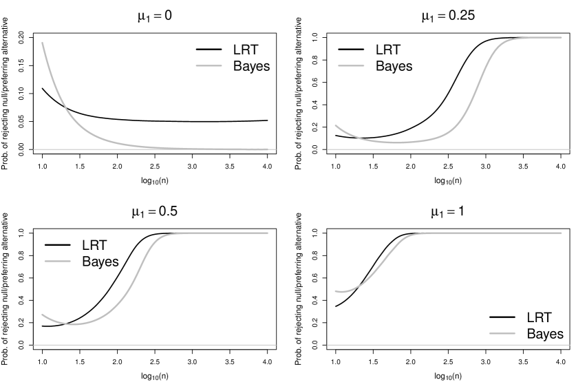
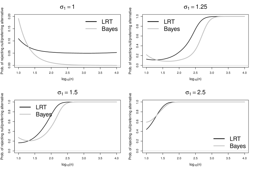
Figure 3: The empirical probabilities of rejecting the null (in the LRT case) or preferring the alternative (in the Bayesian test) when simulating two normal populations with $n_{0}=n_{1}=50$, and (i) $\mu_{0}=0$, $\sigma_{0}=\sigma_{1}=1$ and $\mu_{1}\in\{0,0.25,0.5,1\}$ (left four panels); or (ii) $\mu_{0}=0$, $\mu_{1}=0$, $\sigma_{0}=1$ and $\sigma_{1}\in\{0,1.25,1.5,2.5\}$ (right four panels).

4.3 Linear models

We will now consider hypothesis testing for linear models. Consider the base model

$${\bf y}|\alpha,{\boldsymbol{\beta}},\sigma^{2}\sim N(\alpha{\bf 1}+{\bf X}{\boldsymbol{\beta}},\sigma^{2}{\bf I}),$$

where ${\bf y}$ is a response vector of length $n$, ${\boldsymbol{\beta}}$ is a coefficient vector of length $p$, $\sigma^{2}$ is a positive scalar, ${\bf X}$ is a full-rank $n$ by $p$ matrix of covariates, and ${\bf I}$ is the identity matrix of appropriate dimension. In order to simplify some calculations we will transform ${\bf y}$ and ${\bf X}$ so that ${\bf y}$ and the columns of ${\bf X}$ are standardized, i.e., $\overline{y}=0$, $\|{\bf y}\|^{2}={\bf y}^{T}{\bf y}=n$, ${\bf X}_{j}^{T}{\bf 1}=0$, and $\|{\bf X}_{j}\|^{2}=n$ where ${\bf X}_{j}$ is the $j$th column of ${\bf X}$. Let ${\boldsymbol{\gamma}}$ be a binary vector of length $p$, and let ${\bf X}_{\boldsymbol{\gamma}}$ be the submatrix ${\bf X}$ comprised from the columns of ${\bf X}$ whose corresponding elements of ${\boldsymbol{\gamma}}$ are non-zero. Consider the hypothesis test

$$H_{0}\colon{\boldsymbol{\gamma}}={\boldsymbol{\gamma}}_{0}\qquad\mbox{versus}\qquad H_{1}\colon{\boldsymbol{\gamma}}={\boldsymbol{\gamma}}_{1},$$ (11)

where ${\boldsymbol{\gamma}}_{0}$ and ${\boldsymbol{\gamma}}_{1}$ denote the models under the null and alternative hypotheses respectively with $0\leq|{\boldsymbol{\gamma}}_{0}|\leq|{\boldsymbol{\gamma}}_{1}|$.

To simplify exposition for this example we will only use cake priors for $\alpha$ and ${\boldsymbol{\beta}}_{\boldsymbol{\gamma}}$. Since $\sigma^{2}$ is a common parameter across all parameters we can use the typical improper (Jeffreys) priors for $\sigma^{2}$ given by $p(\sigma^{2})\propto(\sigma^{2})^{-1}{\mathbb{I}}(\sigma^{2}>0)$. This choice has been formally justified in Berger et al. (1998). Cake priors can be used for all parameters for this example, but the working out is lengthy and unnecessarily obfuscates the exposition. Using ${\bf P}(\alpha,{\boldsymbol{\beta}}_{\boldsymbol{\gamma}})=\widetilde{{\mathcal{I}}}(\alpha,{\boldsymbol{\beta}}_{\boldsymbol{\gamma}})=\mbox{diag}(\sigma^{-2},\sigma^{-2}{\bf X}_{\boldsymbol{\gamma}}^{T}{\bf X}_{\boldsymbol{\gamma}}/n)$ for a particular model ${\boldsymbol{\gamma}}$ leads to

$$\alpha|\sigma^{2},g\sim N(0,g\sigma^{2}),\quad\mbox{and}\quad\displaystyle{\boldsymbol{\beta}}_{\boldsymbol{\gamma}}|\sigma^{2},g\sim N\left({\bf 0},g\sigma^{2}\left(\tfrac{1}{n}{\bf X}_{\boldsymbol{\gamma}}^{T}{\bf X}_{\boldsymbol{\gamma}}\right)^{-1}\right).$$ (12)

Further, we use $p({\boldsymbol{\beta}}_{-{\boldsymbol{\gamma}}})=\prod_{j\colon\gamma_{j}=0}\delta(\beta_{j};0)$ where $\delta(x;a)$ is the Dirac delta function with location $a$. The prior on ${\boldsymbol{\beta}}_{\boldsymbol{\gamma}}$ is simply the Zellner $g$-prior (Zellner, 1986) where the prior covariance is scaled by a factor of $n$. The prior on ${\boldsymbol{\beta}}_{\boldsymbol{\gamma}}$ combined with the prior on ${\boldsymbol{\beta}}_{-{\boldsymbol{\gamma}}}$ is a spike and slab prior for ${\boldsymbol{\beta}}$.

Marginalizing over $\alpha$, ${\boldsymbol{\beta}}$ and $\sigma^{2}$ for a particular model ${\boldsymbol{\gamma}}$ we obtain after simplification

$$p({\bf y}|{\boldsymbol{\gamma}},g)=\frac{\Gamma(n/2)}{(n\pi)^{n/2}}\exp\Big{[}-\tfrac{1+|{\boldsymbol{\gamma}}|}{2}\ln(g)-\tfrac{1+|{\boldsymbol{\gamma}}|}{2}\ln(n+g^{-1})-\tfrac{n}{2}\ln\left(1-\tfrac{g}{1+g}R_{{\boldsymbol{\gamma}}}^{2}\right)\Big{]},$$

where $R_{\boldsymbol{\gamma}}^{2}$ is the usual R-squared statistic for model ${\boldsymbol{\gamma}}$. This is equivalent to the $g=h^{1/d_{h}}$ of Section 4 to using the hyperpriors $p(g|{\boldsymbol{\gamma}}_{j})=\delta(g;h^{1/(1+|{\boldsymbol{\gamma}}_{j}|)})$, $j=0,1$. After marginalizing over $g$ the Bayes factor as a function of $h$ simplifies to

$$\begin{array}[]{rl}\displaystyle\mbox{BF}_{01}(h)&\displaystyle=\exp\Big{[}-\tfrac{n}{2}\ln\left(1-\tfrac{h^{1/(1+|{\boldsymbol{\gamma}}_{0}|)}}{1+h^{1/(1+|{\boldsymbol{\gamma}}_{0}|)}}R_{{\boldsymbol{\gamma}}_{0}}^{2}\right)+\tfrac{n}{2}\ln\left(1-\tfrac{h^{1/(1+|{\boldsymbol{\gamma}}_{1}|)}}{1+h^{1/(1+|{\boldsymbol{\gamma}}_{1}|)}}R_{{\boldsymbol{\gamma}}_{1}}^{2}\right)\\[8.61108pt] &\displaystyle\qquad\qquad\qquad-\tfrac{1+|{\boldsymbol{\gamma}}_{0}|}{2}\ln\left(n+h^{-1/(1+|{\boldsymbol{\gamma}}_{0}|)}\right)+\tfrac{1+|{\boldsymbol{\gamma}}_{1}|}{2}\ln\left(n+h^{-1/(1+|{\boldsymbol{\gamma}}_{1}|)}\right)\Big{]}.\end{array}$$

Taking $h\to\infty$ we use the fact that $1-R_{\boldsymbol{\gamma}}^{2}=\widehat{\sigma}_{{\boldsymbol{\gamma}}}^{2}$ (where $\widehat{\sigma}_{{\boldsymbol{\gamma}}}^{2}$ is the MLE for $\sigma^{2}$ under the model ${\boldsymbol{\gamma}}$) to obtain

$$\begin{array}[]{rl}\displaystyle\lambda_{\mbox{\scriptsize Bayes}}&\displaystyle=\left[-n\ln(\widehat{\sigma}_{{\boldsymbol{\gamma}}_{1}}^{2})-|{\boldsymbol{\gamma}}_{1}|\ln(n)\right]-\left[-n\ln(\widehat{\sigma}_{{\boldsymbol{\gamma}}_{0}}^{2})-|{\boldsymbol{\gamma}}_{0}|\ln(n)\right]\\[4.30554pt] &\displaystyle=\mbox{BIC}_{{\boldsymbol{\gamma}}_{0}}-\mbox{BIC}_{{\boldsymbol{\gamma}}_{1}}=\lambda_{\mbox{\scriptsize LRT}}-\nu\ln(n),\end{array}$$

where $\displaystyle\mbox{BIC}_{{\boldsymbol{\gamma}}}=n\ln(2\pi\widehat{\sigma}_{{\boldsymbol{\gamma}}}^{2})-n+|{\boldsymbol{\gamma}}|\ln(n)=-2\ln p({\bf y}|\widehat{\alpha}_{{\boldsymbol{\gamma}}},\widehat{{\boldsymbol{\beta}}}_{{\boldsymbol{\gamma}}},\widehat{\sigma}_{{\boldsymbol{\gamma}}}^{2})+|{\boldsymbol{\gamma}}|\ln(n),$ and, $\widehat{\alpha}_{{\boldsymbol{\gamma}}}$ and $\widehat{{\boldsymbol{\beta}}}_{{\boldsymbol{\gamma}}}$ are the MLEs for $\alpha$ and ${\boldsymbol{\beta}}$ under model ${\boldsymbol{\gamma}}$, $\lambda_{\mbox{\scriptsize LRT}}=n\ln(\widehat{\sigma}_{{\boldsymbol{\gamma}}_{0}}^{2})-n\ln(\widehat{\sigma}_{{\boldsymbol{\gamma}}_{1}}^{2})$ is the LRT statistic corresponding to the hypotheses (11) and $\nu=|{\boldsymbol{\gamma}}_{1}|-|{\boldsymbol{\gamma}}_{0}|$. Hence, for these models and prior structures the Bayesian test statistic is simply the difference between two BIC values.

Note that as $h\to\infty$ the parameter posteriors become

$$\alpha|{\bf y},{\boldsymbol{\gamma}}\sim t_{n}(0,\widehat{\sigma}_{{\boldsymbol{\gamma}}}^{2}/n),\quad{\boldsymbol{\beta}}_{{\boldsymbol{\gamma}}}|{\bf y},{\boldsymbol{\gamma}}\sim t_{n}(\widehat{{\boldsymbol{\beta}}}_{{\boldsymbol{\gamma}}},\widehat{\sigma}_{{\boldsymbol{\gamma}}}^{2}\left({\bf X}_{\boldsymbol{\gamma}}^{T}{\bf X}_{\boldsymbol{\gamma}}\right)^{-1}),\quad\mbox{and}\quad\sigma^{2}|{\bf y},{\boldsymbol{\gamma}}\sim\mbox{IG}\left(\tfrac{n}{2},\tfrac{n}{2}\widehat{\sigma}_{{\boldsymbol{\gamma}}}^{2}\right),$$

where $\widehat{{\boldsymbol{\beta}}}_{{\boldsymbol{\gamma}}}$ and $\widehat{\sigma}_{{\boldsymbol{\gamma}}}^{2}$ are the MLEs corresponding to model ${\boldsymbol{\gamma}}$.

We will not provide any numerical examples due to the close relationship between our Bayes factors and the BIC, and the fact that almost every paper ever written on model selection for linear models uses the BIC in its comparisons. We direct the interested reader to any of the papers in the discussion below all of which make comparisons with the BIC as a model selection criteria.

There are four main differences between the priors used here and the priors that have been used in the literature for linear models. The first such difference is the choice of prior on $\alpha$ which the typical prior is to use the Jeffreys prior $p(\alpha)\propto 1$ which was advocated in Berger et al. (1998). If we were to use this prior and were only to use cake priors for ${\boldsymbol{\beta}}_{\boldsymbol{\gamma}}$ then $p(g_{0}|{\boldsymbol{\gamma}}_{0};h)=\delta(g_{0};h^{1/|{\boldsymbol{\gamma}}_{0}|})$ instead of $p(g_{0}|{\boldsymbol{\gamma}}_{0};h)=\delta(g_{0};h^{1/(1+|{\boldsymbol{\gamma}}_{0}|)})$. The consequence of this would be that the null model (where ${\boldsymbol{\gamma}}={\bf 0}$) would become problematic to calculate.

The second difference is in the choice of prior for ${\boldsymbol{\beta}}$. Most Bayesian approaches to model selection for linear models use the Zellner $g$-prior where

$${\boldsymbol{\beta}}_{\boldsymbol{\gamma}}|\sigma^{2},g\sim N({\bf 0},g\sigma^{2}({\bf X}_{\boldsymbol{\gamma}}^{T}{\bf X}_{\boldsymbol{\gamma}})^{-1}),$$ (13)

instead of the prior for ${\boldsymbol{\beta}}_{\boldsymbol{\gamma}}$ in (12). This difference is subtle.

Bayarri et al. (2012) advocate the priors for ${\boldsymbol{\beta}}$ should remain proper and not degenerate to a point mass. If we were to treat ${\bf X}_{\boldsymbol{\gamma}}$ as random then under mild conditions ${\bf X}_{\boldsymbol{\gamma}}^{T}{\bf X}_{\boldsymbol{\gamma}}/n\to{\mathbb{E}}({\bf X}_{\boldsymbol{\gamma}}^{T}{\bf X}_{\boldsymbol{\gamma}})$ almost surely suggesting that our prior for ${\boldsymbol{\beta}}_{\boldsymbol{\gamma}}$ does not degenerate to a point mass. Lastly (12) and (13) simplify marginal likelihoods since terms involving determinants cancel, and have the added advantage that they do not depend on the unit of measurements of the covariates.

The third difference is the choice of prior on $g$. As stated in the introduction, Liang et al. (2008) argues for a hyperprior to be assigned to $g$. Liang et al. (2008) considers the hyper $g$-prior; the hyper $g/n$-prior; and the Zellner-Siow prior (equivalent to a particular inverse-gamma on $g$) (Zellner and Siow, 1980). Maruyama and George (2011) use a different prior to (12) or (13) and a beta-prime prior with specially chosen prior hyperparameter values. All of these choices, apart from Maruyama and George (2011), either no closed form expression for the marginal likelihood exists, or such an expression is in terms of a Gauss hypergeometric function which is numerically difficult to evaluate (Pearson et al., 2017) so that approximation is required.

Model selection consistency is another desirable criteria of Bayarri et al. (2012). The authors corresponding $g/n$, Zellner-Siow, beta-prior and robust priors are model selection consistent for all possible models. Our prior specification results in a null based Bayes factor is a simple function of the BIC and so achieves model selection consistency for iid data (under some additional mild assumptions, Yang, 2005). See also Section 5.2.

4.4 Handling zero parameters in the null model

Let us now return to Lindley’s example posed by Lindley (1957) described in Section 3. In order to apply the methodology of Section 4 the null model needs to have a non-zero number of parameters. We provide the following novel artificial construct to handle this case in order to augment the problems so that both hypotheses have a non-zero number of parameters.

1. Introduce a second sample of hypothetical data, say ${\bf z}$.

2. Modify the null and alternative hypotheses by adding a clause that the hypothetical data has the same distribution under the null and alternative hypotheses.

3. Apply the methodology of Section 4 to the augmented problem.

In order to illustrate this approach suppose we have a second sample of hypothetical data ${\bf z}=(z_{1},\ldots,z_{n})^{T}$ and consider the augmented hypotheses

$$\begin{array}[]{l}H_{0}\colon x_{1},\ldots,x_{n}\sim N(\mu_{0},\sigma^{2})\qquad\mbox{and}\qquad z_{1},\ldots,z_{n}|\widetilde{\mu}\sim N(\widetilde{\mu},\sigma^{2})\qquad\mbox{versus}\\[4.30554pt] H_{1}\colon x_{1},\ldots,x_{n}|\mu\sim N(\mu,\sigma^{2})\qquad\mbox{and}\qquad z_{1},\ldots,z_{n}|\widetilde{\mu}\sim N(\widetilde{\mu},\sigma^{2}),\end{array}$$

where $\mu_{0}$ and $\sigma^{2}$ have known fixed values, and $\widetilde{\mu}$ is an artificial mean parameter corresponding to the sample ${\bf z}$. This is a modification of the original hypotheses (3) has the same logical implication as the hypotheses (3) for the observed sample ${\bf x}$ since the hypothetical data has the same hypothetical models under the null and alternative hypotheses. For the augmented problem we have ${\boldsymbol{\theta}}_{0}=\widetilde{\mu}$ with $d_{0}=1$, and ${\boldsymbol{\theta}}_{1}=(\mu,\widetilde{\mu})^{T}$ and $d_{1}=2$ so that we have avoided the problem of dividing by zero. The cake priors become $\widetilde{\mu}|H_{0}\sim N(0,g_{0}\sigma^{2})$, $\mu|H_{1}\sim N(0,g_{1}\sigma^{2})$ and $\widetilde{\mu}|H_{1}\sim N(0,g_{1}\sigma^{2}).$ For $g_{0}$ and $g_{1}$ we use $g_{0}=h$ and $g_{1}=h^{1/2}$. Then

$$\begin{array}[]{rl}\ln p({\bf x}|H_{0})\par&\displaystyle=-\tfrac{n}{2}\ln(2\pi\sigma^{2})-\tfrac{\|{\bf x}-\mu_{0}{\bf 1}\|^{2}}{2\sigma^{2}},\par\\[8.61108pt] \ln p({\bf z}|H_{0})&\displaystyle=-\tfrac{n}{2}\ln(2\pi\sigma^{2})-\tfrac{1}{2\sigma^{2}}\left[\|{\bf z}\|^{2}-\tfrac{(n\overline{z})^{2}}{n+h^{-1}}\right]-\tfrac{1}{2}\ln(h)-\tfrac{1}{2}\ln(n+h^{-1}),\par\\[8.61108pt] \ln p({\bf x}|H_{1})&\displaystyle=-\tfrac{n}{2}\ln(2\pi\sigma^{2})-\tfrac{1}{2\sigma^{2}}\left[\|{\bf x}\|^{2}-\tfrac{(n\overline{x})^{2}}{n+h^{-1/2}}\right]-\tfrac{1}{2}\ln(h^{1/2})-\tfrac{1}{2}\ln\left(n+\tfrac{1}{\sqrt{h}}\right),\ \mbox{and}\par\\[8.61108pt] \ln p({\bf z}|H_{1})&\displaystyle=-\tfrac{n}{2}\ln(2\pi\sigma^{2})-\tfrac{1}{2\sigma^{2}}\left[\|{\bf z}\|^{2}-\tfrac{(n\overline{z})^{2}}{n+h^{-1/2}}\right]-\tfrac{1}{2}\ln(h^{1/2})-\tfrac{1}{2}\ln\left(n+\tfrac{1}{\sqrt{h}}\right).\end{array}$$

The Bayes factor in the limit as $h\to\infty$ is

$$\lambda_{\mbox{\scriptsize Bayes}}=\lim_{h\to\infty}-2\ln\left[\frac{p({\bf x}|H_{0})p({\bf z}|H_{0})}{p({\bf x}|H_{1})p({\bf z}|H_{1})}\right]=\lambda_{\mbox{\scriptsize LRT}}-\ln(n),$$

where $\lambda_{\mbox{\scriptsize LRT}}=\sigma^{-2}(\|{\bf x}-\mu_{0}{\bf 1}\|^{2}-\|{\bf x}-\widehat{\mu}{\bf 1}\|^{2})$ is the likelihood ratio test statistic corresponding to the hypothesis (3). We conducted a small simulation study identical to the simulation study in Section 4.1 with the exception that $\sigma^{2}$ was treated as known. The resulting figure and interpretation was nearly identical to that in Section 4.1 (not shown).

5 Theory

In all of the examples in Section 4 the quantity $\lambda_{\mbox{\scriptsize Bayes}}$ can be placed into the form (2). We will now consider the asymptotic properties of hypothesis tests based on this form. Shao (2003) developed theory regarding the asymptotic properties of hypothesis tests. We will adopt his notation and definitions here. Let ${\bf X}=(X_{1},...,X_{n})^{T}$ be a random sample from ${\mathcal{P}}=\{\,p_{i}(\,\cdot\,)\colon i=1,\ldots,n\,\}$. The type I and type II errors are defined by $\alpha_{T}({\mathcal{P}})={\mathbb{P}}(\,T({\bf X})=1)$ when ${\mathcal{P}}\in{\mathcal{P}}_{0}$ and $1-\alpha_{T}({\mathcal{P}})={\mathbb{P}}(\,T({\bf X})=0)$ when ${\mathcal{P}}\in{\mathcal{P}}_{1}$ respectively. Fix the level of significance $\alpha$ such that $\sup_{{\mathcal{P}}\in{\mathcal{P}}_{0}}\{\alpha_{T}({{\mathcal{P}}})\}\leq\alpha$. We will now suppose that $T_{n}({\bf X})\equiv T({\bf X})$ and consider scenarios where $n$ diverges. In our ensuing discussion we use the following definitions.

Definitions from 2.13 of Shao (2003):

1. If $\displaystyle\lim_{n\to\infty}\sup_{{\mathcal{P}}\in{\mathcal{P}}_{0}}\{\alpha_{T_{n}}({\mathcal{P}})\}\leq\alpha$ then $\alpha$ is an asymptotic significance level of $T_{n}$.

2. If $\displaystyle\lim_{n\to\infty}\sup_{{\mathcal{P}}\in{\mathcal{P}}_{0}}\{\alpha_{T_{n}}({\mathcal{P}})\}$ exists, then it is called the limiting size of $T_{n}$.

3. The sequence of tests $T_{n}$ is called consistent if and only if the type II error probability converges to $0$, i.e., $\lim_{n\to\infty}[1-\alpha_{T_{n}}({\mathcal{P}})]=0$, for any ${\mathcal{P}}\in{\mathcal{P}}_{1}$.

4. The sequence of tests $T_{n}$ is called Chernoff-consistent if and only if $T_{n}$ is consistent and the type I error probability converges to 0, i.e., $\lim_{n\to\infty}\{\alpha_{T_{n}}({\mathcal{P}})\}=0$, for any ${\mathcal{P}}\in{\mathcal{P}}_{0}$. Furthermore, $T_{n}$ is called strongly Chernoff-consistent if and only if $T_{n}$ is consistent and the limiting size of $T_{n}$ is $0$.

We note that any reasonable test which is consistent where the level $\alpha$ is controllable, can be made Chernoff-consistent by letting $\alpha_{n}\equiv\alpha\to 0$ as $n\to\infty$.

Wilks Theorem (Wilks, 1938) tells us that, assuming the data was generated under the null distribution, under appropriate regularity conditions (including that the hypotheses are nested) that $\lambda_{\mbox{\scriptsize LRT}}$ converges to $\chi_{\nu}^{2}$ in distribution so that $\lambda_{\mbox{\scriptsize LRT}}=O_{p}(1)$. A detailed exposition on the characterization the asymptotic distribution of the LRT statistic under quite general conditions, including when $H_{0}$ and/or $H_{1}$ is misspecified, and whether the hypotheses are nested or non-nested, can be found in Vuong (1989). Below we summarize the most pertinent results.

5.1 Asymptotic properties of the likelihood ratio test statistic

Suppose $X_{1},X_{2},\ldots,X_{n}$ are independent random variables from $\{\,p_{0i}(\,\cdot\,)\colon i=1,\ldots,n\,\}$ and that we have a parametric model $\mathcal{P}=\{\,p_{i}(\,\cdot\,|{\boldsymbol{\theta}})\colon i=1,\ldots,n,\ {\boldsymbol{\theta}}\in\Theta\,\}$ (which may or may not include the true distribution(s) $\{\,p_{0i}(\,\cdot\,)\,\}$). Define the log-likelihood as $\ell({\boldsymbol{\theta}})=\sum_{i=1}^{n}\ln p_{i}(X_{i}|{\boldsymbol{\theta}})$, the MLE and “pseudo-true” value of ${\boldsymbol{\theta}}$ as

$$\widehat{{\boldsymbol{\theta}}}=\arg\max_{\theta}\,\{\,\ell({\boldsymbol{\theta}})\,\}\qquad\mbox{and}\qquad{\boldsymbol{\theta}}^{*}=\arg\max_{{\boldsymbol{\theta}}}\ \left[{\mathbb{E}}\left\{n^{-1}\ell({\boldsymbol{\theta}})\right\}\right],$$

respectively (assuming both are well-defined). Assume also that ${\mathbb{E}}\left[n^{-1}\ell({\boldsymbol{\theta}}^{*})\right]\to C,$ for some finite $C>0$. Under the “pseudo-true” value ${\boldsymbol{\theta}}^{*}$ the resultant distribution is $\{\,p_{i}(\,\cdot\,|{\boldsymbol{\theta}}^{*})\,\}$ which is the “best” distribution in the sense that it results in the smallest Kullback-Leibler (KL) divergence with respect to the true distribution over all distributions for the model. We assume that these are unique.

If $\mathcal{P}$ is suitably regular, with $\Theta$ a nice subset of $d$-dimensional Euclidean space, then certain derivatives exist and various statements can be made: the Euclidean norm of $\widehat{{\boldsymbol{\theta}}}-{\boldsymbol{\theta}}^{*}$ is $O_{p}(n^{-1/2})$, and writing $\nabla\ell({\boldsymbol{\theta}})$ and $\nabla^{2}\ell({\boldsymbol{\theta}})$ for the first and second order partial derivatives we may expand $\ell({\boldsymbol{\theta}}^{*})$ about $\widehat{{\boldsymbol{\theta}}}$ to get

$$\begin{array}[]{rl}\ell({\boldsymbol{\theta}}^{*})&=\ell(\widehat{{\boldsymbol{\theta}}})+({\boldsymbol{\theta}}^{*}-\widehat{{\boldsymbol{\theta}}})^{T}\nabla\ell(\widehat{{\boldsymbol{\theta}}})+\tfrac{1}{2}({\boldsymbol{\theta}}^{*}-\widehat{{\boldsymbol{\theta}}})^{T}\left[\nabla^{2}\ell(\widetilde{{\boldsymbol{\theta}}})\right]({\boldsymbol{\theta}}^{*}-\widehat{{\boldsymbol{\theta}}})\\ &=\ell(\widehat{{\boldsymbol{\theta}}})-\tfrac{1}{2}\Big{[}n^{1/2}(\widehat{{\boldsymbol{\theta}}}-{\boldsymbol{\theta}}^{*})\Big{]}^{T}{\mathbb{E}}\Big{[}-\tfrac{1}{n}\nabla^{2}\ell({\boldsymbol{\theta}}^{*})\Big{]}\Big{[}n^{1/2}(\widehat{{\boldsymbol{\theta}}}-{\boldsymbol{\theta}}^{*})\Big{]}+o_{p}(1),\end{array}$$

since $\nabla\ell(\widehat{{\boldsymbol{\theta}}})\equiv 0$, for some $\widetilde{{\boldsymbol{\theta}}}$ between ${\boldsymbol{\theta}}^{*}$ and $\widehat{{\boldsymbol{\theta}}}$; also the quadratic form is $O_{p}(1)$. Thus, we may decompose the maximised log-likelihood into the following terms:

$$\ell(\widehat{{\boldsymbol{\theta}}})={\mathbb{E}}\left[\ell({\boldsymbol{\theta}}^{*})\right]+\left[\ell({\boldsymbol{\theta}}^{*})-{\mathbb{E}}\left\{\ell({\boldsymbol{\theta}}^{*})\right\}\right]+O_{p}(1).$$

The first term on the right hand side is asymptotic to $nC$; the second term is a random sum of $n$ terms with expectation zero, and so under further regularity conditions is $O_{p}(n^{1/2})$. We refer to these three terms as the “$O_{p}(n)$”, “$O_{p}(n^{1/2})$” and “$O_{p}(1)$” terms respectively (from left to right). Precise regularity conditions guaranteeing all of this nice behaviour may be found in Vuong (1989); see also Chapter 5 of van der Vaart (1998). They are all easily satisfied in all of our examples.

Finally, we note that the first term can be written as:

$$\begin{array}[]{rl}\displaystyle{\mathbb{E}}\left[\ell({\boldsymbol{\theta}})\right]&\displaystyle={\mathbb{E}}\left[\sum_{i=1}^{n}\ln\left\{\frac{p_{i}(X_{i}|{\boldsymbol{\theta}})}{p_{0i}(X_{i})}\right\}\right]+{\mathbb{E}}\left[\sum_{i=1}^{n}\ln p_{0i}(X_{i})\right]\\ &\displaystyle\widehat{=}-\mbox{KL}(\,p_{0i}\,||\,p_{i}\,)+{\mathbb{E}}\left[\sum_{i=1}^{n}\ln p_{0i}(X_{i})\right]\end{array}$$

where the first term corresponds to the negative KL-divergence between $p_{0i}$ and $p_{i}$, and the second term is related to the entropy of $p_{0i}$. We see from the above equation that maximizing ${\mathbb{E}}\left[\ell({\boldsymbol{\theta}})\right]$ with respect to ${\boldsymbol{\theta}}$ is equivalent to minimizing the KL-divergence between $\prod_{i=1}^{n}p_{0i}(\,\cdot\,)$ and $\prod_{i=1}^{n}p_{i}(\,\cdot\,|{\boldsymbol{\theta}})$.

5.2 Comparing models

Suppose now that we have two competing models $\mathcal{P}_{j}=\{\,p_{ij}(\,\cdot\,|{\boldsymbol{\theta}}_{j},H_{j})\colon i=1,\ldots,n,\ {\boldsymbol{\theta}}_{j}\in\Theta\,\},j=0,1$, with corresponding log-likelihoods $\ell_{0}(\,\cdot\,)$ and $\ell_{1}(\,\cdot\,)$, MLEs $\widehat{{\boldsymbol{\theta}}}_{0}$ and $\widehat{{\boldsymbol{\theta}}}_{1}$, and pseudo-true values ${\boldsymbol{\theta}}_{0}^{*}$ and ${\boldsymbol{\theta}}_{1}^{*}$. For convenience we will write $\widehat{\ell}_{j}\equiv\ell_{j}(\widehat{{\boldsymbol{\theta}}}_{j})$. Suppose also that for $j=0,1$, we have ${\mathbb{E}}\left[n^{-1}\ell_{j}({\boldsymbol{\theta}}_{j}^{*})\right]\to\ell_{j}^{*}$.

There are two main cases:

1. If $\ell_{1}^{*}>\ell_{0}^{*}$ then the model under $H_{1}$ has a smaller KL-divergence from the true distribution than the model under $H_{0}$, and we have immediately

   $$n^{-1}\lambda_{\mbox{\scriptsize LRT}}({\bf X})=n^{-1}(\widehat{\ell}_{1}-\widehat{\ell}_{0})\stackrel{{\scriptstyle P}}{{\to}}\ell_{1}^{*}-\ell_{0}^{*}>0\,,$$

   that is the LRT statistic $\lambda_{\mbox{\scriptsize LRT}}({\bf X})=2(\widehat{\ell}_{1}-\widehat{\ell}_{0})$ is of order $n$ in probability.

2. If $\ell_{1}^{*}=\ell_{0}^{*}$ then immediately we see that the two “$O_{p}(n)$” terms in the difference between the log-likelihoods would, at least asymptotically, cancel out and that the “$O_{p}(n^{1/2})$” terms would “dominate”. However, in many practical examples the “$O_{p}(n^{1/2})$” terms also cancel out, in which case

   $$\lambda_{\mbox{\scriptsize LRT}}({\bf X})=2(\widehat{\ell}_{1}-\widehat{\ell}_{0})=O_{p}(1)\,.$$

   (see in particular Theorem 3.3 of Vuong, 1989). This occurs when the “best” member of each model yields the same distribution, that is when $\{\,p_{i0}(\,\cdot\,|{\boldsymbol{\theta}}_{0}^{*},H_{0})\,\}=\{\,p_{i1}(\,\cdot\,|{\boldsymbol{\theta}}_{1}^{*},H_{1})\,\}$. The parametrisations may be completely different, but nonetheless the distributions corresponding to the pseudo-true parameter values are identical. This occurs when the two models have some overlap, i.e., $\mathcal{P}_{0}\cap\mathcal{P}_{1}$ is non-empty as a subset of all possible sets of distributions $\{\,p_{i}(\,\cdot\,)\,\}$. In such a case, the models may or may not be nested, and may or may not be correctly specified; however the “best” distribution in both is the same (and is part of the overlap).

We also have the following consequences.

• Lindley’s paradox: If $H_{1}$ is correct (and $H_{0}$ is not) then the above theory implies $\lambda_{\mbox{\scriptsize LRT}}({\bf X})$ is $O_{p}(n)$ and a test of the form (2) is consistent. Since Lindley’s paradox occur with asymptotic probability $p(\chi_{\nu,\alpha}^{2}<\lambda_{\mbox{\scriptsize LRT}}<\nu\ln n)$, it occurs with vanishingly small probability as $n\to\infty$.

• Chernoff-consistency: If $H_{0}$ is true then $\lambda_{\mbox{\scriptsize LRT}}({\bf X})$ is $O_{p}(1)$ and ${\mathbb{P}}(T({\bf X})=1)\to 0$ as $n\to\infty$. If $H_{1}$ is true then $\lambda_{\mbox{\scriptsize LRT}}({\bf X})$ is $O_{p}(n)$ and ${\mathbb{P}}(T({\bf X})=0)\to 0$ as $n\to\infty$. Hence, a Bayesian test of the form (2) is Chernoff consistent.

• Model selection consistency: Now suppose that we have $M$ competing hypotheses $H_{j}$, $j=1,\ldots,M$. For each model we have ${\mathbb{E}}\left[n^{-1}\ell_{j}({\boldsymbol{\theta}}_{j}^{*})\right]\to\ell_{j}^{*}$ for some constants $\ell_{j}^{*}$. We will call a hypothesis $H_{j}$ correct if $j\in{\mathcal{C}}$ where

  $${\mathcal{C}}=\Big{\{}\,j\,\colon\,\ell_{j}^{*}=\max_{k=1,\ldots,M}\ell_{k}^{*}\,\Big{\}}.$$

  The hypotheses $H_{j}$ such that $j\in{\mathcal{C}}$ correspond to correct models in the sense that all such models are closest in terms of their KL-divergence to the data generating distribution. Using (2) to compare models not in ${\mathcal{C}}$ with models in ${\mathcal{C}}$ leads to $\lambda_{\mbox{\scriptsize LRT}}({\bf X})$ is $O_{p}(n)$ and the test preferring the model in ${\mathcal{C}}$. Comparing any two models in ${\mathcal{C}}$ will asymptotically prefer the model with the smallest size.

When cake priors become arbitrarily diffuse to the point of becoming improper and a further problem occurs. We now discuss such problems.

6 Arbitrary constants

We now return to the issue of improper priors in the context of Bayes factors discussed in the introduction. When using improper priors, consider the conditional density $p({\bf x}|{\boldsymbol{\theta}}_{i},H_{j})$ where $p({\boldsymbol{\theta}}|H_{j})\propto f_{i}({\boldsymbol{\theta}}_{j})=D_{j}f_{j}({\boldsymbol{\theta}}_{j})$ for some $D_{j}>0$ such that $\int f_{j}({\boldsymbol{\theta}}_{j})d{\boldsymbol{\theta}}_{j}$ does not exist for $j=0,1$. Then

$$B_{01}=\frac{D_{0}}{D_{1}}\times\frac{\int p({\bf x}|{\boldsymbol{\theta}},H_{0})f_{0}({\boldsymbol{\theta}}_{0})d{\boldsymbol{\theta}}_{0}}{\int p({\bf x}|{\boldsymbol{\theta}},H_{1})f_{1}({\boldsymbol{\theta}}_{1})d{\boldsymbol{\theta}}_{1}}.$$ (14)

This Bayes factor is problematic since it depends on two arbitrary constants $D_{0}$ and $D_{1}$.

• Problem III: When using improper priors either the null or the alternative model can be made to be preferred by artificially changing $D_{0}$ or $D_{1}$ to suit the a priori preferred conclusion.

In the limit as as $h\to\infty$ cake priors become improper. Suppose that instead of using $g_{j}=h_{j}^{1/d_{j}}$ we use $g_{j}=(D_{j}h)^{1/d_{j}}$, where $c_{j}>0$ are arbitrary constants. This implies

$$\lambda_{\mbox{\scriptsize Bayes}}=\lambda_{\mbox{\scriptsize LRT}}-\nu\ln(n)+\Delta+o_{p}(1)$$

where $\Delta=\ln(D_{1}/D_{0})$ is a controllable constant determined by how the $g_{j}$ parameters diverge. Thus, we have not avoided the problem of arbitrary constants in our test.

Based on the theory developed in Section 5, if $\Delta=O(1)$ then the corresponding test will have all of the properties discussed in Section (5.2) where the level of the test requires adjustment. For small sample sizes the value of $\Delta$ trades-off the probabilities of type I and type II errors. We do not believe that the model nor the data can make the choice of $\Delta$ value on behalf of the analyst. Furthermore, any criteria used to select $\Delta$ is making the choice in trade-off of relative probabilities of type I and type II errors whether implicitly or explicitly. Implicitly cake priors are choosing $\Delta=0$.

This choice might be preferred for the following reasons:

1. This choice leads to a parsimonious expression for $\lambda_{\mbox{\scriptsize Bayes}}$ (all $O(1)$ terms cancel);

2. When the number of parameters in the null and alternative hypotheses are equal ($\nu=0$) using $\Delta=0$ leads to preferring the model with the larger likelihood. If $\Delta\neq 0$ this is always the case. If the analyst desired to explicitly favour ether model when $\nu=0$ then the prior odds should be altered to achieve this; and

3. Choosing different values of $D_{0}$ and $D_{1}$ would be inconsistent with similar choices made in the literature. For example, in the linear models example one might also use $p(\alpha^{2}|H_{j})=D_{j}$ or $p(\sigma^{2}|H_{j})=D_{j}(\sigma^{2})^{-1}I(\sigma^{2}>0)$. No papers in the model selection literature, to our knowledge, chose different constants $D_{j}$ for each model under consideration. This suggests choosing $D_{0}=D_{1}$ is reasonable.

Lastly, we note that if we select $\Delta=\nu\ln(n)-\chi_{\nu,\alpha}^{2}$, where $\chi_{\nu,\alpha}^{2}$ denotes the upper quantile function of the chi-squared distribution with degrees of freedom parameter $\nu$, that Bayesian tests can be made to mimic the frequentists LRT when the type I error is controlled to have level $\alpha$.

7 Interpretation

For Bayesian test using cake priors and the LRT test functions are (approximately)

$$T_{\mbox{\scriptsize Bayes}}({\bf x})=I(\lambda_{\mbox{\scriptsize LRT}}({\bf x})>\nu\ln(n))\qquad\mbox{and}\qquad T_{\mbox{\scriptsize LRT}}({\bf x})=I(\lambda_{\mbox{\scriptsize LRT}}({\bf x})>\chi_{\nu,\alpha}^{2})$$ (15)

respectively. This also allows us to obtain a one-to-one mapping between $p$-values and values of $\lambda_{\mbox{\scriptsize Bayes}}({\bf x})$. It can be shown

$$\nu+2\ln(1/\alpha)-5/2\leq\chi_{\nu,\alpha}^{2}\leq\nu+2\ln(1/\alpha)+2\sqrt{\nu\ln(1/\alpha)},$$ (16)

where the lower bound only holds for $\alpha\leq 0.17$ and $\nu\geq 2$ (Laurent and Massart, 2000; Inglot, 2010). For our Bayesian tests the cut-off value, $\nu\ln(n)$ grows with $n$ implying that the level of the test decays with $n$. A consequence is that our Bayesian tests offer some protection against a sequential analysis (where samples are collected and statistical significance checked sequentially). Suppose that $\alpha=(n/e)^{\nu/2}$ then (16) becomes $\displaystyle\nu\ln(n)-5/2\leq\chi_{\nu,\alpha}^{2}\leq\nu\ln(n)+\sqrt{2\nu^{2}\ln(n)}$ so that $\chi_{\nu,\alpha}^{2}\asymp\nu\ln(n)$, and the frequentist and Bayesian testing procedures are roughly equivalent.

Given that (15) we can directly compare that the Bayes factors have taken the interpretation offered by Kass and Raftery (1995) in Table 1 appears to have the short-coming of not taking into account the degrees of freedom $\nu$ of the test, nor the sample size $n$. Consider Table 2 which directly compares $p$-values with their corresponding $\lambda_{\mbox{\scriptsize Bayes}}$ for given $n$ and $\nu$. If one were to use a LRT instead where $\lambda_{\mbox{\scriptsize Bayes}}({\bf x})$ takes the threshold values in Table 1, i.e., $\lambda_{\mbox{\scriptsize Bayes}}({\bf x})\in\{0,2,6,10\}$, $\nu$ ranges from 1 to 5, and $n\in\{50,10^{2},10^{3}\}$. Note that every $p$-value is smaller than 5% suggesting that Bayesian tests are typically more conservative at preferring the alternative than classical tests reject the null at the usual 5% cut-off. Further, going from $\lambda_{\mbox{\scriptsize Bayes}}({\bf x})=2$ to $\lambda_{\mbox{\scriptsize Bayes}}({\bf x})=6$ and from $\lambda_{\mbox{\scriptsize Bayes}}=6$ to $\lambda_{\mbox{\scriptsize Bayes}}({\bf x})=10$ roughly translates to a 5 to 10 fold reduction in the corresponding $p$-value. Thus, the anticipated potential short-coming of Table 1 not depending on $\nu$ or $n$ does not pan out, at least for the values of $n$ and $\nu$ considered in Table 2. We believe Table 2 is a reasonable interpretation of strength of evidence for Bayesian tests.

		$p$-values
$\nu$	$\lambda_{\mbox{\tiny Bayes}}$	$n=50$	$n=10^{2}$	$n=10^{3}$
1	0	4.79E-02	3.18E-02	8.58E-04
1	2	1.50E-02	1.02E-02	2.84E-03
1	6	1.64E-03	1.13E-03	3.27E-04
1	10	1.92E-04	1.33E-04	3.92E-05
2	0	2.00E-02	1.00E-02	1.00E-03
2	2	7.36E-03	3.68E-03	3.68E-04
2	6	9.96E-04	4.98E-04	4.98E-05
2	10	1.35E-04	6.74E-05	6.74E-06
3	0	8.34E-02	3.16E-03	1.20E-04
3	2	3.29E-03	1.24E-03	4.61E-05
3	6	4.99E-04	1.85E-04	6.73E-06
3	10	7.40E-05	2.73E-05	9.72E-07
4	0	3.53E-03	1.02E-03	1.48E-05
4	2	1.45E-03	4.12E-04	5.82E-06
4	6	2.35E-04	6.58E-05	8.87E-07
4	10	3.73E-05	1.02E-05	1.34E-07

	$\lambda_{\mbox{\scriptsize Bayes}}$
$p$-value	$n=50$	$n=10^{2}$	$n=10^{3}$
0.05	$-$0.1	$-$0.8	$-$3.1
0.01	2.7	2.0	$-$0.3
0.001	6.9	6.2	3.9
0.0001	11.2	10.5	8.2
0.05	$-$1.8	$-$3.2	$-$7.8
0.01	1.4	0.0	$-$4.6
0.001	6.0	4.6	0.0
0.0001	10.6	9.2	4.6
0.05	$-$3.9	$-$6.0	$-$12.9
0.01	$-$0.4	$-$2.5	$-$9.4
0.001	4.5	2.5	$-$4.5
0.0001	9.4	7.3	0.4
0.05	$-$6.2	$-$8.9	$-$18.1
0.01	$-$2.4	$-$5.1	$-$14.4
0.001	2.8	0.0	$-$9.2
0.0001	7.9	5.1	$-$4.1

Table 2: The third to sixth columns are LRT based $p$-value for the $\lambda_{\mbox{\scriptsize Bayes}}\in\{0,2,6,10\}$ specified in the second column for different values of $n$ and $\nu$. The eighth to 11th colums are values of $\lambda_{\mbox{\scriptsize Bayes}}$ for the $p$-value specified in the seventh column for different values of $n$ and $\nu$.

8 Conclusion

We have introduced a new class of priors we call cake priors having a number of desirable properties. Cake priors can be made arbitrarily diffuse without the Bayes factor favouring the null or alternative hypotheses as the prior becomes increasingly diffuse. In the limit, at least for the examples we consider here, Bayes factors take the form of penalized likelihood ratio statistics, one of the most thoroughly understood quantities in Statistics. Due to their close link with Jeffreys priors, cake priors are parametrization invariant. The resulting Bayesian test avoids the need to specify a $p$-value cut-off and are asymptotically Chernoff-consistent. With a slight modification, an arbitrary but controllable constant can be used to bridge the gap between Bayesian tests and likelihood ratio tests. Unlike approaches that split the dataset up into parts or use imaginary data, cake priors are transparent, uncomplicated, and easily implementable. Finally, Bayesian tests using cake priors providing some protection against sequential testing being more conservative as the sample size grows. We believe all of the above properties should make cake priors the default choice when performing Bayesian hypothesis tests for hypothesis consisting of a simple point null against a composite alternative for parametric models with iid data.

References

• Abramowitz and Stegun (1972) Abramowitz, M., Stegun, I. A., 1972. Handbook of Mathematical Functions with Formulas, Graphs, and Mathematical Tables. New York: Dover Publications.
• Aitkin (1991) Aitkin, M., 1991. Posterior Bayes factors (with discussion). Journal of the Royal Statistical Society, Series B 53 (1), 111–142.
• Bartlett (1957) Bartlett, M. S., 1957. A comment on D.V. Lindley’s statistical paradox. Biometrika 44 (3), 533–534.
• Bayarri et al. (2012) Bayarri, M. J., Berger, J. O., Forte, A., García-Donato, G., 2012. Criteria for Bayesian model choice with application to variable selection. The Annals of Statistics 40 (3), 1550–1577.
• Berger and Pericchi (1996) Berger, J. O., Pericchi, L. R., 1996. The intrinsic Bayes factor for model selection and prediction. Journal of the American Statistical Association 91 (433), 109–122.
• Berger and Pericchi (2001) Berger, J. O., Pericchi, L. R., 2001. Objective Bayesian methods for model selection: Introduction and comparison. IMS Lecture Notes - Monograph Series 38, 135–207.
• Berger et al. (1998) Berger, J. O., Pericchi, L. R., Varshavsky, J. A., 1998. Bayes factors and marginal distributions in invariant situations. Sankhyā: The Indian Journal of Statistics, Series A 60 (3), 307–321.
• Bernardo (1980) Bernardo, J. M., 1980. A Bayesian analysis of classical hypothesis testing. Trabajos de Estadistica Y de Investigacion Operativa 31 (1), 605–647.
• Bernardo (1999) Bernardo, J. M., 1999. Nested hypothesis testing: The Bayesian reference criterion. Bayesian Statistics, 101–130.
• Bové and Held (2011) Bové, D. S., Held, L., 2011. Hyper-$g$ priors for generalized linear models. Bayesian Analysis 6 (3), 387–410.
• Chen et al. (2008) Chen, M. H., Huang, L., Ibrahim, J. G., Kim, S., 2008. Bayesian variable selection and computation for generalized linear models with conjugate priors. Bayesian Analysis 3 (3), 585–614.
• Chen and Ibrahim (2003) Chen, M. H., Ibrahim, J. G., 2003. Conjugate priors for generalized linear models. Statistica Sinica 13 (2), 461–476.
• DeGroot (1973) DeGroot, M. H., 1973. Doing what comes naturally: Interpreting a tail area as a poterior probability or as a likelihood ratio. Journal of the American Statistical Association 68, 966–969.
• Fernández et al. (2001) Fernández, C., Ley, E., Steel, M. F. J., 2001. Benchmark priors for Bayesian model averaging. Journal of Econometrics 100 (2), 381 – 427.
• Gelman et al. (2013) Gelman, A., Carlin, J. B., Stern, H. S., Dunson, D. B., Vehtari, A., Rubin, D. B., 2013. Bayesian Data Analysis, 3rd Edition. Chapman & Hall/CRC Texts in Statistical Science. Taylor & Francis.
• Gelman et al. (1996) Gelman, A., Meng, X.-L., Stern, H., 1996. Posterior predictive assessment of model fitness via realized discrepancies. Statistica Sinica 6 (4), 733–760.
• George and McCulloch (1993) George, E. I., McCulloch, R. E., 1993. Variable selection via Gibbs sampling. Journal of the American Statistical Association 88 (423), 881–889.
• Good (1952) Good, I. J., 1952. Rational decisions. Journal of the Royal Statistical Society, Series B 14 (1), 107–114.
• Gupta and Ibrahim (2009) Gupta, M., Ibrahim, J. G., 2009. An information matrix prior for Bayesian analysis in generalized linear models with high dimensional data. Statistica Sinica 19 (4), 1641–1663.
• Hansen and Yu (2001) Hansen, M. H., Yu, B., 2001. Model selection and the principle of minimum description length. Journal of the American Statistical Association 96 (454), 746–774.
• Hanson et al. (2014) Hanson, T. E., Branscum, A. J., Johnson, W. O., 2014. Informative g-priors for logistic regression. Bayesian Analysis 9 (3), 597–612.
• Inglot (2010) Inglot, T., 2010. Inequalities for quantiles of the chi-square distribution. Probability and Mathematical Statistics 30 (2), 339–351.
• Jahn et al. (1987) Jahn, R. G., Dunne, B. J., Nelson, R. D., 1987. Engineering anomalies research. Journal of Scientific Exploration 1 (1), 583–639.
• Jeffreys (1935) Jeffreys, H., 1935. Some tests of significance, treated by the theory of probability. Mathematical Proceedings of the Cambridge Philosophical Society 31 (2), 203–222.
• Jeffreys (1946) Jeffreys, H., 1946. An invariant form for the prior probability in estimation problems. Proceedings of the Royal Society of London A: Mathematical, Physical and Engineering Sciences 186 (1007), 453–461.
• Jeffreys (1961) Jeffreys, H., 1961. Theory of Probability. Vol. 2. Oxford University Press.
• Kass and Raftery (1995) Kass, R. E., Raftery, A., 1995. Bayes Factors. Journal of the American Statistical Association 91 (6), 773–795.
• Kass et al. (1990) Kass, R. E., Tierney, L., Kadane, J. B., 1990. The validity of posterior expansions based on Laplace’s method. In: Geisser, S., Hodges, J. S., S.J. Press, S. J., Zellner, A. (Eds.), Essays in Honor of George Bernard. North Holland, pp. 473–488.
• Laurent and Massart (2000) Laurent, B., Massart, P., 10 2000. Adaptive estimation of a quadratic functional by model selection. The Annals of Statistics 28 (5), 1302–1338.
• Lehmann (2004) Lehmann, E., 2004. Elements of Large-Sample Theory. Springer Texts in Statistics. Springer New York.
• Li and Clyde (2015) Li, Y., Clyde, M. A., 2015. Mixture of g-priors in generalized linear models., arXiv preprint arXiv:1503.06913.
• Liang et al. (2008) Liang, F., Paulo, R., Molina, G., Clyde, M. A., Berger, J. O., 2008. Mixtures of $g$-priors for Bayesian variable selection. Journal of the American Statistical Association 103 (481), 410–423.
• Lindley (1957) Lindley, D. V., 1957. A statistical paradox. Biometrika 44, 187–192.
• Maruyama and George (2011) Maruyama, Y., George, E. I., 2011. Fully Bayes factors with a generalized $g$-prior. The Annals of Statistics 39 (5), 2740–2765.
• Mitchell and Beauchamp (1988) Mitchell, T. J., Beauchamp, J. J., 1988. Bayesian variable selection in linear regression. Journal of the American Statistical Association 83, 1023–1032.
• Naaman (2016) Naaman, M., 2016. Almost sure hypothesis testing and the resolution of the Jeffreys-Lindey paradox. Electronic Journal of Statistics 19, 1526–1550.
• O’Hagan (1995) O’Hagan, A., 1995. Fractional Bayes factors for model comparison. Journal of the Royal Statistical Society, Series B 57 (1), 99–138.
• O’Hagan (1997) O’Hagan, A., 1997. Properties of intrinsic and fractional Bayes factors. Test 6, 101–118.
• Pearson et al. (2017) Pearson, J. W., Olver, S., Porter, M. A., 2017. Numerical methods for the computation of the confluent and Gauss hypergeometric functions. Numerical Algorithms 74, 821–866.
• Pettit (1992) Pettit, L. I., 1992. Bayes factors for outlier models using the device of imaginary observations. Journal of the American Statistical Association 87, 541–545.
• Robert (1993) Robert, C. P., 1993. A note on Jeffreys-Lindley paradox. Statistica Sinica 3, 601–608.
• Robert (2014) Robert, C. P., 2014. On the Jeffreys-Lindley paradox. Philosophy of Science 81 (2), 216–232.
• Schwarz (1978) Schwarz, G., 1978. Estimating the dimension of a model. The Annals of Statistics 6 (2), 461–464.
• Shao (2003) Shao, J., 2003. Mathematical Statistics. Springer Texts in Statistics. Springer.
• Smith and Spiegelhalter (1980) Smith, A. F. M., Spiegelhalter, D. J., 1980. Bayes factors and choice criteria for linear models. Journal of the Royal Statistical Society, Series B 42 (2), 213–220.
• Spanos (2013) Spanos, A., 2013. Who should be afraid of the Jeffreys-Lindley paradox? Philosophy of Science 80 (1), 73–93.
• Spiegelhalter et al. (2002) Spiegelhalter, D. J., Best, N. G., Carlin, B. P., van der Linde, A., 2002. Bayesian measures of model complexity and fit. Journal of the Royal Statistical Society, Series B 64 (4), 583–639.
• Spiegelhalter and Smith (1982) Spiegelhalter, D. J., Smith, A. F. M., 1982. Bayes factors for linear and log-linear models with vague prior information. Journal of the Royal Statistical Society, Series B 44 (3), 377–387.
• Sprenger (2013) Sprenger, J., 2013. Testing a precise null hypothesis: The case of Lindley’s paradox. Philosophy of Science 80 (5), 733–744.
• Tierney et al. (1989) Tierney, L., Kass, R. E., Kadane, J. B., 1989. Fully exponential Laplace approximations to expectations and variances of nonpositive functions. Journal of the American Statistical Association 84 (407), 710–716.
• van der Vaart (1998) van der Vaart, A. W., 1998. Asymptotic statistics, volume 3 of Cambridge Series in Statistical and Probabilistic Mathematics. Cambridge University Press, Cambridge.
• Vuong (1989) Vuong, Q. H., 1989. Likelihood ratio tests for model selection and nonnested hypotheses. Econometrica 57 (2), 307–333.
• Wang and George (2007) Wang, X., George, E. I., 2007. Adaptive Bayesian criteria in variable selection for generalized linear models. Statistics Sinica 17, 667–690.
• Wilks (1938) Wilks, S. S., 1938. The large-sample distribution of the likelihood ratio for testing composite hypotheses. The Annals of Mathematical Statistics 9 (1), 60–62.
• Yang (2005) Yang, Y., 2005. Can the strengths of AIC and BIC be shared? A conflict between model indentification and regression estimation. Biometrika 92 (4), 937.
• Zellner (1986) Zellner, A., 1986. On assessing prior distributions and Bayesian regression analysis with $g$-prior distributions. Bayesian Inference and Decision Techniques: Essays in Honor of Bruno de Finetti, 233–243.
• Zellner and Siow (1980) Zellner, A., Siow, A., 1980. Posterior odds ratios for selected regression hypotheses. Trabajos de Estadistica Y de Investigacion Operativa 31 (1), 585–603.