Sharp-interface limits of a phase-field model with a generalized Navier slip boundary condition for moving contact lines

Abstract

The sharp-interface limits of a phase-field model with a generalized Navier slip boundary condition for moving contact line problem are studied by asymptotic analysis and numerical simulations. The effects of the mobility number as well as a phenomenological relaxation parameter in the boundary condition are considered. In asymptotic analysis, we focus on the case that the mobility number is the same order of the Cahn number and derive the sharp-interface limits for several setups of the boundary relaxation parameter. It is shown that the sharp interface limit of the phase field model is the standard two-phase incompressible Navier-Stokes equations coupled with several different slip boundary conditions. Numerical results are consistent with the analysis results and also illustrate the different convergence rates of the sharp-interface limits for different scalings of the two parameters.

1 Introduction

Moving contact lines are common in nature and our daily life, e.g. the motion of rain drops on window glass, coffee rings left by evaporation of coffee drops, wetting on lotus leaves, etc. The moving contact line problem also has many applications in some industrial processes, like painting, coating and oil recovery, etc. Therefore, the problem has been studied extensively. see recent review papers by Pismen (2002); Blake (2006); Bonn et al. (2009); Snoeijer & Andreotti (2013) and the references therein.

Moving contact line is a challenging problem in fluid dynamics. The standard two-phase Navier-Stokes equations with a no-slip boundary condition will lead to a non-physical non-integrable stress (Huh & Scriven, 1971; Dussan, 1979). This is the so-called contact line paradox. There are many efforts to solve this paradox. A natural way is to relax the no-slip boundary condition. Instead, one could use the Navier slip boundary condition (Huh & Scriven, 1971; Cox, 1986; Zhou & Sheng, 1990; Haley & Miksis, 1991; Spelt, 2005; Ren & E, 2007). In some applications, an effective slip condition can be induced by numerical methods (Renardy et al., 2001; Marmottant & Villermaux, 2004). The other approaches to cure the paradox include: to assume a precursor thin film and a disjoint pressure (Schwartz & Eley, 1998; Pismen & Pomeau, 2000; Eggers, 2005); to derive a new thermodynamics for surfaces (Shikhmurzaev, 1993); to treat the moving contact line as a thermally activated process (Blake, 2006; Blake & De Coninck, 2011; Seveno et al., 2009), to use a diffuse interface model for moving contact lines (Seppecher, 1996; Gurtin et al., 1996; Jacqmin, 2000; Qian et al., 2003; Yue & Feng, 2011a), etc.

The diffuse interface approach for moving contact lines has become popular recent years (Anderson et al., 1998; Qian et al., 2004; Ding & Spelt, 2007; Carlson et al., 2009; Ren & E, 2011; Sibley et al., 2013b; Sui et al., 2014; Shen et al., 2015; Fakhari & Bolster, 2017). In this approach, the interface is a thin diffuse layer between different fluids represented by a phase field function. Intermolecular diffusion, caused by the non-equilibrium of the chemical potential, occurs in the thin layer. The chemical diffusion can cause the motion of the contact line, even without using a slip boundary condition on the solid boundary (Jacqmin, 2000; Chen et al., 2000; Briant et al., 2004; Yue & Feng, 2011b; Sibley et al., 2013c). On the other hand, it is possible to combine the diffuse interface model with some slip boundary condition. Qian, Wang & Sheng (2003) proposed a phase-field model with a generalized Navier slip boundary condition (GNBC). The model takes account of the effect of the uncompensated Young stress, which is important to understand the difference of the dynamic contact angle and the Young’s angle in molecular scale (Qian et al., 2003; Ren & E, 2007). Theoretically, the model can be derived from the Onsager variational principle (Qian et al., 2006). Numerical simulations using this model fit remarkably well with the molecular dynamics simulations (Qian et al., 2003) and physical experiments (Guo et al., 2013). The model has also been used in problems with chemically patterned boundaries (Wang et al., 2008), dynamic wetting problems (Carlson et al., 2009; Yamamoto et al., 2014), etc. Several numerical methods for the model have been developed (Gao & Wang, 2012; Bao et al., 2012; Gao & Wang, 2014; Shen et al., 2015; Aland & Chen, 2015).

Phase field models are convenient for numerical calculations  (Yue et al., 2004; Teigen et al., 2011; Sui et al., 2014). One does not need to track the interface explicitly as in using a sharp interface model. The phase-field function, which usually described by a Cahn-Hilliard (Cahn & Hilliard, 1958) equation or an Allen-Cahn equation (Allen & Cahn, 1979), can capture the interface implicitly and automatically. This makes computations and analysis for the phase field model much easier than other approaches. However, there are also some restrictions to use a diffuse interface model in real simulations. A key issue is that the thickness of the diffuse interface can not be chosen as small as the physical size (Khatavkar et al., 2006), due to the restriction of the computational resources. One often choose a much larger (than physical values) interface thickness parameter(or a dimensionless Cahn number) in simulations. But, only when phase field model approximates a sharp-interface limit correctly, the numerical simulations by this model with relatively large Cahn number can be trustful and compared with experiments quantitatively. Therefore, it is very important to study the sharp-interface limit of a phase field model (Caginalp & Chen, 1998; Chen et al., 2014).

The sharp-interface limits of diffuse interface models for two-phase flow without moving contact lines has been studied a lot, both theoretically and numerically (Lowengrub & Truskinovsky, 1998; Jacqmin, 1999; Khatavkar et al., 2006; Huang et al., 2009; Magaletti et al., 2013; Sibley et al., 2013a). In comparison, there are much less studies for the sharp-interface limit of the phase field models for moving contact lines (Yue et al., 2010; Kusumaatmaja et al., 2016). One important progress is made by Yue, Zhou & Feng (2010). They studied the sharp interface limit of a phase field model with a no-slip boundary condition and found a surprising result that only when the mobility parameter (denoted as $\mathsf{L_{d}}$) is of order $O(1)$, the phase field model has a sharp-interface limit as the Cahn number (denoted as $\varepsilon$) goes to zero. Notice that the usual choice of the mobility parameter is of order $O(\varepsilon^{\beta})$, $1\leq\beta\leq 3$ for problems without moving contact lines (Magaletti et al., 2013). For the phase field model with the generalized Navier slip boundary condition, the only study for its sharp interface limit is done by Wang & Wang (2007). They also assumed the mobility parameter is of order $O(1)$. Their asymptotic analysis shows that the sharp-interface limit of the model is a Hele-Shaw flow coupled with a standard Navier-slip boundary condition. So far, it is not clear what is the sharp-interface limit of a phase field model for moving contact line problem under the standard choice for the mobility parameter, e.g. $\mathsf{L_{d}}=O(\varepsilon)$. This is the motivation of our study.

We study the sharp-interface limit of the phase field model with the GNBC by asymptotic analysis and numerical simulations. In asymptotic analysis, we assume that the mobility number $\mathsf{L_{d}}$ is of order $O(\varepsilon)$ and consider several typical scalings of phenomenological boundary relaxation parameter $\mathsf{V_{s}}$ in the GNBC model. We show that the sharp-interface limit is a standard two-phase Navier-Stokes equations coupled with different slip boundary conditions for different choices of $\mathsf{V_{s}}$. When $\mathsf{V_{s}}=O(\varepsilon^{\beta})$ with $\beta=0,-1$, we obtain a sharp-interface version of the GNBC. In the case $\mathsf{V_{s}}=O(1)$, the velocity of the contact line is equal to the fluid velocity, while in the case $\mathsf{V_{s}}=O(\varepsilon^{-1})$, the velocity of the contact line is different from the fluid velocity due to the contribution of the chemical diffusion on the boundary. When $\mathsf{V_{s}}=O(\varepsilon^{-2})$, we obtain the standard Navier slip boundary condition together with the condition that the dynamic contact angle is equal to the static contact angle. Numerical experiments for a Couette flow show the different sharp-interface limits for the various choice of $\mathsf{L_{d}}$ and $\mathsf{V_{s}}$. Furthermore, numerical results also reveal the different convergence rates for different choices of the two parameters. For very large relaxation parameter $\mathsf{V_{s}}=O(\varepsilon^{-3})$, the numerical results are very similar to the results by Yue, Zhou & Feng (2010).

The structure of the paper is as follows. In Section 2, we introduce the phase field model with the GNBC and its non-dimensionalization. In Section 3, the sharp-interface limits of the phase field model with the GNBC are obtained for various choice of $\mathsf{V_{s}}$ by asymptotic analysis. In Section 4, we show the numerical experiments for a Couette flow by a recent developed second order scheme. Finally, some concluding remarks are given in Section 5.

2 The phase field model with generalized Navier slip boundary condition

A Cahn-Hilliard-Navier-Stokes (CHNS) system with the generalized Navier boundary condition (GNBC) is proposed by Qian, Wang & Sheng (2003) to describe a two-phase flow with moving contact lines. The CHNS system reads

$$\left\{\begin{array}[]{ll}\frac{\partial\phi}{\partial t}+\mathbf{v}\cdot\nabla\phi=M\Delta\mu,\qquad\qquad\mu=-K\Delta\phi-r(\phi-\phi^{3}),&\hbox{}\\ \rho[\frac{\partial\mathbf{v}}{\partial t}+(\mathbf{v}\cdot\nabla)\mathbf{v}]=\mathbf{F}-\nabla p+\eta\Delta\mathbf{v}+\mu\nabla\phi,\quad\nabla\cdot\mathbf{v}=0.&\hbox{}\end{array}\right.$$ (1)

The first equation is the Cahn-Hilliard equation. Here $\phi$ is the phase field function, and $\mu$ is the chemical potential. The thickness of the diffuse interface is $\xi=\sqrt{K/r}$ and the fluid-fluid interface tension is given by $\gamma=2\sqrt{2}r\xi/3$. $M$ is a phenomenological mobility coefficient. The second equation in (1) is the incompressible Navier-Stokes equation for two-phase flow. Here $\mu\nabla\phi$ describes the capillary force exerted to the fluids by the interface. For simplicity, we assume that the two fluids have equal density $\rho$ and viscosity $\eta$.

The generalized Navier boundary condition on the solid boundary is

$$\beta(v_{\tau}-v_{w})=-\eta\partial_{n}v_{\tau}+L(\phi)\partial_{\tau}\phi, \quad v_{n}=0,$$ (2)

$$L(\phi)=K\partial_{n}\phi+\frac{\partial\gamma_{wf}(\phi)}{\partial\phi}, \gamma_{wf}(\phi)=-\frac{\gamma}{4}\cos\theta_{s}(3\phi-\phi^{3}).$$ (3)

Here $v_{n}$ and $v_{\tau}$ are respectively the normal fluid velocity and the tangential fluid velocity on the solid boundary. $v_{w}$ is the velocity of the boundary itself. We assume the wall only moves in a tangential direction. $\beta$ is a slip coefficient and the slip length is given as $l_{s}=\eta/\beta$.$\gamma_{wf}(\phi)$ is the solid-fluid interfacial energy density (up to a constant) and $\theta_{s}$ is the static contact angle. $L(\phi)\partial_{\tau}\phi$ represents the uncompensated Young stress.

In addition, the boundary conditions for the phase field $\phi$ and the chemical potential $\mu$ are given by

$$\begin{array}[]{l}\frac{\partial\phi}{\partial t}+v_{\tau}\partial_{\tau}\phi=-\Gamma L(\phi),\\ \partial_{n}\mu=0,\end{array}$$ (4)

with $\Gamma$ being a positive phenomenological relaxation parameter.

To study the behavior of the CHNS system with the GNBC condition, it is useful to nondimensionalize the system. Suppose the typical length scale in the two-phase flow system is given by $l$ and the characteristic velocity is $v^{*}$. We then scale the velocity by $v^{*}$, the length by $l$, the time by $l/v^{*}$, body force(density) $\mathbf{F}$ by $\eta v^{*}/l^{2}$ and the pressure by $\eta v^{*}/l$. With six dimensionless parameters:

$$\mathsf{L_{d}}=\frac{3M\gamma}{2\sqrt{2}v^{*}l^{2}}\hbox{ (the mobility number)}, \mathsf{R_{e}}=\frac{\rho v^{*}l}{\eta}\hbox{ (the Reynold number)},$$

$$\mathsf{B}=\frac{3\gamma}{2\sqrt{2}\eta v^{*}}\hbox{ (inverse of the Capillary number)}, \mathsf{V_{s}}=\frac{3\gamma\Gamma l}{2\sqrt{2}v^{*}}\hbox{ (a relaxation parameter)},$$

$$\mathsf{l_{s}}=\frac{l_{s}}{l}\hbox{ (the dimensionless slip length)}, \varepsilon=\frac{\xi}{l}\hbox{ (the Cahn number)},$$

we have the following dimensionless Cahn-Hilliard-Navier-Stokes system

$$\left\{\begin{array}[]{ll}\frac{\partial\phi}{\partial t}+\mathbf{v}\cdot\nabla\phi=\mathsf{L_{d}}\Delta\mu,\qquad\mu=-\varepsilon{\Delta}{\phi}-{\phi}/\varepsilon+{\phi}^{3}/\varepsilon,&\\ \mathsf{R_{e}}\Big{[}\frac{\partial\mathbf{v}}{\partial t}+(\mathbf{v}\cdot\nabla)\mathbf{v}\Big{]}=\mathbf{F}-\nabla{p}+{\Delta}{\mathbf{v}}+\mathsf{B}\mu{\nabla}{\phi},&\hbox{}\\ {\nabla}\cdot{\mathbf{v}}=0,&\hbox{}\end{array}\right.$$ (8)

with the boundary conditions

$$\left\{\begin{array}[]{ll}\frac{\partial{\phi}}{\partial{t}}+{{v}}_{\tau}{\partial_{\tau}}{\phi}=-\mathsf{V_{s}}\mathcal{L}(\phi),&\hbox{}\\ \mathsf{l_{s}}^{-1}({v}_{\tau}-v_{w})=-\partial_{n}{v}_{\tau}+\mathsf{B}\mathcal{L}(\phi)\partial_{\tau}{\phi},&\hbox{}\\ \partial_{n}\mu=0,\ \ \ \ {v}_{n}=0,&\hbox{}\end{array}\right.$$ (9)

where $\mathcal{L}(\phi)=\varepsilon\partial_{n}{\phi}+\frac{\partial\gamma_{wf}(\phi)}{\partial\phi}$ and $\gamma_{wf}(\phi)=-\frac{\sqrt{2}}{6}\cos\theta_{s}(3\phi-\phi^{3})$ being the wall-fluid interfacial energy density function. We now clarify some notations in the boundary condition. Suppose the unit outward normal vector on the solid boundary is given by $\mathbf{n}_{S}$ (see Figure 1). Then, we have $v_{n}=\mathbf{v}\cdot\mathbf{n}_{S}$, $v_{\tau}=\mathbf{v}-v_{n}\mathbf{n}_{S}$, $\partial_{n}=\mathbf{n}_{S}\cdot\nabla$ and $\partial_{\tau}=\nabla-\mathbf{n}_{S}(\mathbf{n}_{S}\cdot\nabla)$.

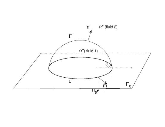
Figure 1: A liquid drop on a planar solid surface $\Gamma_{S}$ with a contact line $L$.

3 The asymptotic analysis

We do asymptotic analysis for the Cahn-Hilliard-Navier-Stokes system (8)-(9). Here we assume the mobility number satisfies $\mathrm{L_{d}}=O(\varepsilon)$.We show that such a choice of mobility will also lead to the standard two-phase Navier-Stokes equation inside the domain. Furthermore, this assumption also makes it possible to derive proper boundary conditions for the sharp-interface limit of the diffuse-interface model. We show that different setups of the relaxation parameter $\mathsf{V_{s}}=O(\varepsilon^{\beta})$, $\beta=0,-1,-2$ will lead to different boundary conditions.

To make the presentation in this section clear, we use $\phi_{\varepsilon}$, $\mathbf{v}_{\varepsilon}$ and $p_{\varepsilon}$ instead of $\phi$, $\mathbf{v}$ and $p$ in the system (8)-(9), to show explicitly that these functions depend on $\varepsilon$. We suppose that the system is located in a domain $\Omega$ with solid boundary $\Gamma_{S}{\subseteq}\partial\Omega$ (as shown in Figure 1). Suppose that the two-phase interface is given by the zero level-set of the phase field function $\phi_{\varepsilon}$

$$\Gamma:=\{x\in\Omega\ |\ \phi_{\varepsilon}(x)=0\}.$$ (10)

We denote by $\Omega^{-}=\{x\in\Omega\,|\,\phi_{\varepsilon}<0\}$ the domain occupied by fluid 1 and $\Omega^{+}=\{x\in\Omega\,|\,\phi_{\varepsilon}>0\}$ the domain occupied by fluid 2.

3.1 The bulk equations

We first do asymptotic analysis for the Cahn-Hilliard-Navier-Stokes system far from the boundary. The analysis is the same as that for two-phase flow without contact lines. We will state the key steps of the analysis and illustrate the main results. In the next subsection, the bulk analysis here will be combined with the analysis near the boundary to derive the sharp-interface limits of the GNBC.

Let $\mathrm{L_{d}}=\varepsilon l_{d}$. Consider the CHNS system far from the boundary of $\Omega$. We first do outer expansions far from the interface $\Gamma$, then we consider inner expansions near $\Gamma$. Combining them together, we will obtain the sharp-interface limit of the CHNS system in $\Omega$.

Outer expansions. Far from the two-phase interface $\Gamma$, we use the following ansatz,

$$\begin{array}[]{l}\mathbf{v}_{\varepsilon}^{\pm}=\mathbf{v}_{0}^{\pm}+\varepsilon\mathbf{v}_{1}^{\pm}+\varepsilon^{2}\mathbf{v}_{2}^{\pm}+\cdots,\\ \phi_{\varepsilon}^{\pm}=\phi_{0}^{\pm}+\varepsilon\phi_{1}^{\pm}+\varepsilon^{2}\phi_{2}^{\pm}+\cdots,\\ p_{\varepsilon}^{\pm}=p_{0}^{\pm}+\varepsilon p_{1}^{\pm}+\varepsilon^{2}p_{2}^{\pm}+\cdots.\end{array}$$ (11)

Here $f^{\pm}$ denotes the restriction of a function $f$ in $\Omega^{+}$ and $\Omega^{-}$ respectively. For $\mu_{\varepsilon}$, we easily have

$$\mu_{\varepsilon}^{\pm}=\varepsilon^{-1}\mu_{0}^{\pm}+\mu_{1}^{\pm}+\varepsilon\mu_{2}^{\pm}+\cdots,$$

where

$$\mu_{0}^{\pm}=-\phi_{0}^{\pm}+(\phi_{0}^{\pm})^{3}.$$ (12)

We substitute the above expansions to the CHNS system (8). The leading order of the first equation of (8) gives

$$\frac{\partial\phi^{\pm}_{0}}{\partial t}+\mathbf{v}_{0}\cdot\nabla\phi_{0}^{\pm}=l_{d}\Delta\mu_{0}^{\pm}.$$ (13)

The leading order of the second equation of (8) gives

$$\mu_{0}^{\pm}\nabla\phi_{0}^{\pm}=0.$$ (14)

More precisely, we have

$$(-\phi_{0}^{\pm}+(\phi_{0}^{\pm})^{3})\nabla\phi_{0}^{\pm}=\nabla(\frac{(1-(\phi_{0}^{\pm})^{2})^{2}}{4})=0.$$

This implies that

$$\phi_{0}^{\pm}=c_{\pm}\qquad\qquad\text{in }\Omega^{\pm},$$ (15)

where $c_{\pm}$ are two constants such that $c_{+}>0$ and $c_{-}<0$. For the third equation of (8), in the leading order, we have

$${\nabla}\cdot{\mathbf{v}_{0}^{\pm}}=0.$$ (16)

By direct calculations, we also have the next order of the second equation of (8) as

$$\mathsf{R_{e}}\Big{[}\frac{\partial\mathbf{v}_{0}^{\pm}}{\partial t}+(\mathbf{v}_{0}^{\pm}\cdot\nabla)\mathbf{v}_{0}^{\pm}\Big{]}=\mathbf{F}-\nabla{p}_{0}^{\pm}+{\Delta}{\mathbf{v}_{0}^{\pm}}+\mu_{0}^{\pm}\nabla\phi_{1}^{\pm}.$$ (17)

Here we have used the fact that $\phi_{0}^{\pm}$ are constants in $\Omega^{\pm}$.

Inner expansions. The outer expansion in $\Omega^{+}$ and $\Omega^{-}$ are connected by the transition layer near the interface $\Gamma$. We will consider the so-called inner expansions near $\Gamma$. Let $d(x,t)$ be signed distance to $\Gamma$, which is well-defined near the interface. Then the unit normal of the interface pointing to $\Omega^{+}$ is given by $\mathbf{n}=\nabla d$. We introduce a new rescaled variable

$$\xi=\frac{d(x)}{\varepsilon}.$$

For any function $f(x)$ (e.g. $f=\mathbf{v}_{\varepsilon},p_{\varepsilon},\phi_{\varepsilon}$), we can rewrite it as

$$f(x)=\tilde{f}(x,\xi).$$ (18)

Then we have

$$\begin{array}[]{l}\nabla f=\nabla\tilde{f}+\varepsilon^{-1}\partial_{\xi}\tilde{f}\mathbf{n},\\ \Delta f=\Delta\tilde{f}+\varepsilon^{-1}\partial_{\xi}\tilde{f}\kappa+2\varepsilon^{-1}(\mathbf{n}\cdot\nabla)\partial_{\xi}\tilde{f}+\varepsilon^{-2}\partial_{\xi\xi}\tilde{f},\\ \partial_{t}f=\partial_{t}\tilde{f}+\varepsilon^{-1}\partial_{\xi}\tilde{f}\partial_{t}d_{\varepsilon}.\end{array}$$ (19)

Here we use the fact that $\nabla\cdot\mathbf{n}=\kappa$, the mean curvature of the interface. $\kappa(x)$ for $x\in\Gamma(t)$ is positive (resp. negative) if the domain $\Omega_{-}$ is convex (resp. concave) near $x$.

In the inner region, we assume that

$$\begin{array}[]{l}\tilde{\mathbf{v}}_{\varepsilon}=\tilde{\mathbf{v}}_{0}+\varepsilon\tilde{\mathbf{v}}_{1}+\varepsilon^{2}\tilde{\mathbf{v}}_{2}+\cdots,\\ \tilde{\phi}_{\varepsilon}=\tilde{\phi}_{0}+\varepsilon\tilde{\phi}_{1}+\varepsilon^{2}\tilde{\phi}_{2}+\cdots,\\ \tilde{p}_{\varepsilon}=\tilde{p}_{0}+\varepsilon\tilde{p}_{1}+\varepsilon^{2}\tilde{p}_{2}+\cdots.\end{array}$$ (20)

A direct expansion for the chemical potential $\tilde{\mu}_{\varepsilon}$ gives

$$\tilde{\mu}_{\varepsilon}=\varepsilon^{-1}\tilde{\mu}_{0}+\tilde{\mu}_{1}+\varepsilon\tilde{\mu}_{2}+\cdots,$$

with

$$\tilde{\mu}_{0}=-\partial_{\xi\xi}\tilde{\phi}_{0}-\tilde{\phi}_{0}+\tilde{\phi}_{0}^{3},$$ (21)

$$\tilde{\mu}_{1}=-\partial_{\xi\xi}\tilde{\phi}_{1}-\partial_{\xi}\tilde{\phi}_{0}\kappa+2(\mathbf{n}\cdot\nabla)\partial_{\xi}\tilde{\phi}_{0}-\tilde{\phi}_{1}+3\tilde{\phi}_{0}^{2}\tilde{\phi}_{1}.$$ (22)

We substitute the above expansions into the system (8). Using the fact that $\mathrm{L_{d}}=\varepsilon l_{d}$, in the leading order, we have

$$\left\{\begin{array}[]{l}\partial_{\xi\xi}\tilde{\mu}_{0}=0,\\ \partial_{\xi\xi}\tilde{\mathbf{v}}_{0}+{\mathsf{B}}\tilde{\mu}_{0}\partial_{\xi}\tilde{\phi}_{0}\mathbf{n}=0,\\ \mathbf{n}\cdot\partial_{\xi}\tilde{\mathbf{v}}_{0}=0.\end{array}\right.$$ (23)

The next order is

$$\left\{\begin{array}[]{l}\partial_{t}d\partial_{\xi}\tilde{\phi}_{0}+\tilde{\mathbf{v}}_{0}\cdot\mathbf{n}\partial_{\xi}\tilde{\phi}_{0}=l_{d}(\partial_{\xi\xi}\tilde{\mu}_{1}+\kappa\partial_{\xi}\tilde{\mu}_{0}+2(\mathbf{n}\cdot\nabla)\partial_{\xi}\tilde{\mu}_{0}),\\ \tilde{\mathbf{v}}_{0}\cdot\mathbf{n}\partial_{\xi}\tilde{\mathbf{v}}_{0}=-\partial_{\xi}\tilde{p}_{0}\mathbf{n}+\partial_{\xi\xi}\tilde{\mathbf{v}}_{1}+\partial_{\xi}\mathbf{\tilde{v}}_{0}\kappa+2(\mathbf{n}\cdot\nabla)\partial_{\xi}\tilde{\mathbf{v}}_{0}+{\mathsf{B}}(\tilde{\mu}_{1}\partial_{\xi}\tilde{\phi}_{0}\mathbf{n}+\tilde{\mu}_{0}\partial_{\xi}\tilde{\phi}_{1}\mathbf{n}+\tilde{\mu}_{0}\nabla\tilde{\phi}_{0}),\\ \mathbf{n}\cdot\partial_{\xi}\tilde{\mathbf{v}}_{1}+\nabla\cdot\tilde{\mathbf{v}}_{0}=0.\end{array}\right.$$ (24)

Matching conditions. We need the following matching conditions for inner and outer expansions.

$$\lim_{\xi\rightarrow\pm\infty}\tilde{f}_{i}(x,\xi)=f_{i}^{\pm}(x),$$ (25)

$$\lim_{\xi\rightarrow\pm\infty}(\nabla_{x}\tilde{f}_{i}(x,\xi)+\partial_{\xi}\tilde{f}_{i+1}(x,\xi)\mathbf{n})=\nabla f_{i}^{\pm}(x).$$ (26)

In the following, we will derive the sharp-interface limit of the CHNS system (8) by the above inner and outer expansions. From the first equation of (23), we know that $\tilde{\mu}_{0}$ is a linear function of $\xi$, which can be written as $\tilde{\mu}_{0}(\xi)=c_{1}\xi+c_{0},$ where $c_{0}$ and $c_{1}$ are independent of $\xi$. Since $\lim_{\xi\rightarrow\pm\infty}\tilde{\mu}_{0}=\mu^{\pm}$ is bounded, we have $c_{1}=0$. Therefore

$$\tilde{\mu}_{0}=c_{0}.$$ (27)

Then the second equation of (23) is reduced to

$$\partial_{\xi\xi}\tilde{\mathbf{v}}_{0}+{\mathsf{B}}c_{0}\partial_{\xi}\tilde{\phi}_{0}\mathbf{n}=0.$$

We integrate the equation with respect to $\xi$ in $(-\infty,\infty)$ and obtain

$$\partial_{\xi}\tilde{\mathbf{v}}_{0}|_{-\infty}^{\infty}+{\mathsf{B}}c_{0}\tilde{\phi}_{0}|_{-\infty}^{\infty}\mathbf{n}=0.$$

The inner product of the equation with $\mathbf{n}$ gives

$$\mathbf{n}\cdot\partial_{\xi}\tilde{\mathbf{v}}_{0}|_{-\infty}^{\infty}+{\mathsf{B}}c_{0}\tilde{\phi}_{0}|_{-\infty}^{\infty}=0.$$

By the third equation of (23), we obtain that

$$c_{0}\tilde{\phi}_{0}|_{-\infty}^{\infty}=0.$$

By the matching condition, we have

$$c_{0}(\phi_{0}^{+}-\phi_{0}^{-})=0.$$

Notice that $c_{+}=\phi_{0}^{+}>0>\phi_{0}^{-}=c_{-}$, we immediately have $c_{0}=0$, or equivalently

$$\tilde{\mu}_{0}=0.$$ (28)

By the equation (21), we have

$$-\partial_{\xi\xi}\tilde{\phi}_{0}-\tilde{\phi}_{0}+\tilde{\phi}_{0}^{3}=0.$$ (29)

The solvability condition for this equation (Pego, 1989) leads to

$$\lim_{\xi\rightarrow\pm\infty}\tilde{\phi}_{0}=\pm 1.$$ (30)

And the solution of (29) is

$$\tilde{\phi}_{0}=\tanh(\xi/\sqrt{2}).$$ (31)

This is the profile of the $\tilde{\phi}_{0}$ in the diffuse-interface layer. By the matching condition $\lim_{\xi\rightarrow\pm\infty}\tilde{\phi}_{0}=\phi_{0}^{\pm}$ and (15), we have

$$\phi_{0}^{\pm}(x)=c_{\pm}=\pm 1,\qquad\hbox{ in }\Omega^{\pm}.$$ (32)

This will lead to $\mu_{0}^{\pm}=0$. Therefore the equation (17) is reduced to

$$\mathsf{R_{e}}\Big{(}\frac{\partial\mathbf{v}_{0}^{\pm}}{\partial t}+(\mathbf{v}_{0}^{\pm}\cdot\nabla)\mathbf{v}_{0}^{\pm}\Big{)}=\mathbf{F}-\nabla{p}_{0}^{\pm}+{\Delta}{\mathbf{v}_{0}^{\pm}}.$$ (33)

Together with (16), this is the standard incompressible Navier-Stokes equation in $\Omega^{\pm}$.

We then derive the jump conditions on the interface $\Gamma$. Noticing (28), the second equation of (23) is reduced to

$$\partial_{\xi\xi}\tilde{\mathbf{v}}_{0}=0.$$

By similar argument as for $\tilde{\mu}_{0}$ in (27), we know that $\tilde{\mathbf{v}}_{0}$ is independent of $\xi$, or

$$\tilde{\mathbf{v}}_{0}(x,\xi)=\tilde{\mathbf{v}}_{0}(x).$$ (34)

By the matching condition for $\tilde{\mathbf{v}}_{0}$, we obtain

$$[\mathbf{v}_{0}]=0,$$ (35)

where $[f]=f^{+}-f^{-}$ denotes the jump of a function $f$ across the interface $\Gamma$. The equation (35) implies that the velocity is continuous across $\Gamma$.

Similarly, the first equation of (24) is reduced to

$$\partial_{t}d\partial_{\xi}\tilde{\phi}_{0}+\tilde{\mathbf{v}}_{0}\cdot\mathbf{n}\partial_{\xi}\tilde{\phi}_{0}=l_{d}\partial_{\xi\xi}\tilde{\mu}_{1}.$$

Integrate the equation in $(-\infty,\infty)$ and use the matching condition for $\tilde{\phi}_{0}$ and $\tilde{\mu}_{1}$, then we obtain

$$\partial_{t}d+\tilde{\mathbf{v}}_{0}\cdot\mathbf{n}=0.$$

This implies that the normal velocity of the interface $\Gamma$ is

$$V_{n}=\mathbf{v}_{0}\cdot\mathbf{n}.$$ (36)

We then show the jump condition for the viscous stress. Noticing (28) and (34), the second equation of (24) can be reduced to

$$-\partial_{\xi}\tilde{p}_{0}\mathbf{n}+\partial_{\xi\xi}\tilde{\mathbf{v}}_{1}+{\mathsf{B}}\mu_{1}\partial_{\xi}\tilde{\phi}_{0}\mathbf{n}=0.$$ (37)

By the equation (22), we have

$$\int_{-\infty}^{\infty}\tilde{\mu}_{1}\partial_{\xi}\tilde{\phi}_{0}d\xi=-\int_{-\infty}^{\infty}(\partial_{\xi}\tilde{\phi}_{0})^{2}d\xi\kappa+\int_{-\infty}^{\infty}(-\partial_{\xi\xi}\tilde{\phi}_{1}-\tilde{\phi}_{1}+3\tilde{\phi}_{0}^{2}\tilde{\phi}_{1})\partial_{\xi}\tilde{\phi}_{0}d\xi.$$ (38)

Integration by parts for the second term in the right hand side of the equation leads to

$$\int_{-\infty}^{\infty}(-\partial_{\xi\xi}\tilde{\phi}_{1}-\tilde{\phi}_{1}+3\tilde{\phi}_{0}^{2}\tilde{\phi}_{1})\partial_{\xi}\tilde{\phi}_{0}d\xi=\int_{-\infty}^{\infty}(\partial_{\xi\xi}\tilde{\phi}_{0}+\tilde{\phi}_{0}-\tilde{\phi}_{0}^{3})\partial_{\xi}\tilde{\phi}_{1}d\xi=0.$$

Here we use the equation (29). Then (38) is reduced to

$$\int_{-\infty}^{\infty}\tilde{\mu}_{1}\partial_{\xi}\tilde{\phi}_{0}d\xi=-\sigma\kappa,$$

with $\sigma=\int_{-\infty}^{\infty}(\partial_{\xi}\tilde{\phi}_{0})^{2}d\xi=\int_{-\infty}^{\infty}(\partial_{\xi}\tanh(\xi/\sqrt{2}))^{2}d\xi=2\sqrt{2}/3$. Then we integrate the equation (37) on $\xi$ in $(-\infty,\infty)$, and notice the matching condition

$$\lim_{\xi\rightarrow\pm\infty}\tilde{p}=p^{\pm},\quad\lim_{\xi\rightarrow\pm\infty}\partial_{\xi}\tilde{\mathbf{v}}_{1}=\mathbf{n}\cdot\nabla\mathbf{v}_{0}^{\pm}.$$

We are led to

$$[-p_{0}\mathbf{n}+(\mathbf{n}\cdot\nabla)\mathbf{v}_{0}]={\mathsf{B}}\sigma\kappa\mathbf{n}.$$

This is the jump condition for pressure and stress (Magaletti et al., 2013).

Combining the above analysis, in the leading order, we obtain the standard Navier-Stokes equation for two-phase immiscible flow

$$\left\{\begin{array}[]{ll}\mathsf{R_{e}}\Big{(}\frac{\partial\mathbf{v}_{0}^{\pm}}{\partial t}+(\mathbf{v}_{0}^{\pm}\cdot\nabla)\mathbf{v}_{0}^{\pm}\Big{)}=\mathbf{F}-\nabla{p}_{0}^{\pm}+{\Delta}{\mathbf{v}_{0}^{\pm}},&\hbox{ in }\Omega^{\pm},\\ \nabla\cdot\mathbf{v}_{0}^{\pm}=0,&\hbox{ in }\Omega^{\pm},\\ \big{[}\mathbf{v}_{0}\big{]}=0,&\hbox{ on }\Gamma,\\ \big{[}-p_{0}\mathbf{n}+(\mathbf{n}\cdot\nabla)\mathbf{v}_{0}\big{]}={\mathsf{B}}\sigma\kappa\mathbf{n},&\hbox{ on }\Gamma,\\ V_{n}=\mathbf{v}_{0}\cdot\mathbf{n},&\hbox{ on }\Gamma.\end{array}\right.$$ (39)

3.2 The boundary conditions

We now consider the sharp-interface limit of the boundary condition (9). We consider three different choices for the relaxation parameter $\mathrm{V_{s}}=O(\varepsilon^{\beta})$, $\beta=0,-1,-2$. We show that they correspond to different boundary conditions in the sharp-interface limit.

Case I. $\mathrm{V_{s}}=O(1)$. We first assume that $\mathrm{V_{s}}$ is a constant independent of the Cahn number $\varepsilon$.

Outer expansion. Far from the moving contact line, we can use the same outer expansions as in the bulk. By applying the expansions (11) to (9) and considering the leading order terms, we easily have the Navier slip boundary condition

$$\mathsf{l_{s}}^{-1}({v}_{0,\tau}-v_{w})=-\partial_{n}{v}_{0,\tau},\quad\mathbf{v}_{0}\cdot\mathbf{n}_{S}=0,\qquad\hbox{on }\Gamma_{S}^{\pm}.$$ (40)

Here ${v}_{0,\tau}=\mathbf{v}_{0}-(\mathbf{v}_{0}\cdot\mathbf{n}_{S})\mathbf{n}_{S}$ is the tangential velocity, and $\Gamma_{S}^{\pm}=\Gamma_{S}\cap\partial\Omega^{\pm}$ is the boundary of $\Omega^{\pm}$ on the solid surface $\Gamma_{S}$. For the chemical potential $\mu$, we have

$$\partial_{n}\mu^{\pm}_{0}=0.$$ (41)

Notice that $\mu_{0}^{\pm}=0$ and $\phi^{\pm}_{0}=\pm 1$ in $\Omega^{\pm}$, we easily obtain

$$\phi_{0}^{\pm}=\pm 1,\quad\mu_{0}^{\pm}=0,\qquad\hbox{on }\Gamma_{S}^{\pm}.$$

Inner expansion. We consider the boundary condition near the contact line. Here we denote the out normal of the solid surface $\Gamma_{S}$ by $\mathbf{n}_{S}$, the normal of the contact line in tangential surface of $\Gamma_{S}$ by $\mathbf{m}$ (as shown in Fig. 1). Since the functions at the contact line need to be matched to the outer expansions on $\Gamma_{S}^{\pm}$ and also to the expansions inside the domain $\Omega$, it is convenient to introduce a different inner expansion near the contact line $L:=\{x\in\Gamma_{S}\,|\,\phi_{\varepsilon}=0\}$ as follows. Near the contact line, we introduce two fast changing parameters,

$$\varrho=\frac{(x-x_{0})\cdot\mathbf{m}}{\varepsilon},\qquad\zeta=\frac{(x-x_{0})\cdot\mathbf{n_{S}}}{\varepsilon},$$

with $x_{0}\in L$. For any function $f(x)$, near $x_{0}$, it can be written as a function in $(x,\rho,\zeta)$ as

$$f(x)=\hat{f}(x,\varrho,\zeta).$$ (42)

The derivative of $f$ is then rewritten as

$$\nabla f =\nabla\hat{f}+\varepsilon^{-1}\mathbf{n}_{S}\partial_{\zeta}\hat{f}+\varepsilon^{-1}\mathbf{m}\partial_{\varrho}\hat{f},$$

$$\Delta f =\Delta\hat{f}+\varepsilon^{-1}(\nabla\cdot\mathbf{n}_{S}\partial_{\zeta}\hat{f}+\nabla\cdot\mathbf{m}\partial_{\varrho}\hat{f}+2\partial_{n\zeta}\hat{f}+2\partial_{m\varrho}\hat{f})+\varepsilon^{-2}(\partial_{\zeta\zeta}\hat{f}+\partial_{\varrho\varrho}\hat{f}),$$

and the boundary derivative of $f$ is given by

$${\partial_{n}f}=\partial_{n}\hat{f}+\varepsilon^{-1}\partial_{\zeta}\hat{f},\qquad\partial_{\tau}f=\partial_{\tau}\hat{f}+\varepsilon^{-1}\partial_{\varrho}\hat{f}\mathbf{m}.$$

We also have

$$\partial_{t}f=\partial_{t}\hat{f}-\varepsilon^{-1}\partial_{\varrho}\hat{f}\partial_{t}x_{0}\cdot\mathbf{m}.$$

Similarly as before, we assume that

$$\hat{\mathbf{v}}_{\varepsilon} =\hat{\mathbf{v}}_{0}+\varepsilon\hat{\mathbf{v}}_{1}+\varepsilon^{2}\hat{\mathbf{v}}_{2}+\cdots,$$

$$\hat{\phi}_{\varepsilon} =\hat{\phi}_{0}+\varepsilon\hat{\phi}_{1}+\varepsilon^{2}\hat{\phi}_{2}+\cdots.$$

Direct computations give

$$\hat{\mu}_{\varepsilon}=\varepsilon^{-1}\hat{\mu}_{0}+\hat{\mu}_{1}+\cdots,$$

with $\hat{\mu}_{0}=-(\partial_{\zeta\zeta}+\partial_{\varrho\varrho})\hat{\phi}_{0}-\hat{\phi}_{0}+\hat{\phi}_{0}^{3},$ and

$$\hat{\mathcal{L}}=\hat{\mathcal{L}}_{0}+\varepsilon\hat{\mathcal{L}}_{1}+\cdots,$$

with $\hat{\mathcal{L}}_{0}=\partial_{\zeta}\hat{\phi}_{0}+\frac{\partial\gamma_{wf}}{\partial\phi}(\hat{\phi}_{0})$.

Substitute the expansions into the CHNS system (8) and the boundary condition (9). In the leading order we have the following equation

$$\left\{\begin{array}[]{ll}(\partial_{\zeta\zeta}+\partial_{\varrho\varrho})\hat{\mu}_{0}=0,&\hbox{}\\ {\mathsf{B}}\hat{\mu}_{0}(\partial_{\zeta}\hat{\phi}_{0}\mathbf{n}_{S}+\partial_{\varrho}\hat{\phi}_{0}\mathbf{m})+(\partial_{\zeta\zeta}+\partial_{\varrho\varrho})\hat{\mathbf{v}}_{0}=0,&\hbox{}\\ \mathbf{n}_{S}\cdot\partial_{\zeta}\hat{\mathbf{v}}_{0}+\mathbf{m}\cdot\partial_{\varrho}\hat{\mathbf{v}}_{0}=0,&\hbox{}\end{array}\right.$$ (43)

and the boundary condition on $\Gamma_{S}$:

$$\left\{\begin{array}[]{ll}-\partial_{t}x_{0}\cdot\mathbf{m}+{\hat{v}}_{0,\tau}\cdot\mathbf{m}=0,&\hbox{}\\ \varepsilon\mathrm{l_{s}}^{-1}(\hat{v}_{0,\tau}-v_{w})+\varepsilon\partial_{n}\hat{v}_{0,\tau}+\partial_{\zeta}\hat{v}_{0,\tau}=\mathsf{B}\hat{\mathcal{L}}_{0}\partial_{\varrho}\hat{\phi}_{0},&\hbox{}\\ \partial_{\zeta}\hat{\mu}_{0}=0,\qquad\hat{\mathbf{v}}_{0}\cdot\mathbf{n}_{S}=0.&\hbox{}\end{array}\right.$$ (44)

Here in the second equation of (44), we keep the terms $\varepsilon\mathrm{l_{s}}^{-1}(\hat{v}_{0,\tau}-v_{w})+\varepsilon\partial_{n}\hat{v}_{0,\tau}$, since the slip velocity in the vicinity of the moving contact line might be large compared with the out region (Qian et al., 2004).

Matching condition. We have the matching condition

$$\lim_{\zeta\rightarrow+\infty}\hat{f}=\lim_{x\rightarrow x_{0}}\tilde{f}(x,\xi),$$

$$\lim_{\varrho\rightarrow\pm\infty}\hat{f}=\lim_{x\rightarrow x_{0}}f^{\pm}(x).$$

In the following, we will use these equations to derive the condition for moving contact lines. By the matching relation for $\mu$,

$$\lim_{\zeta\rightarrow+\infty}\hat{\mu}_{0}=\tilde{\mu}_{0}=0,\qquad\lim_{\varrho\rightarrow\pm\infty}\hat{\mu}_{0}=\mu^{\pm}=0.$$

The first equation of (43) implies that

$$\hat{\mu}_{0}=0.$$ (45)

This means

$$-(\partial_{\zeta\zeta}+\partial_{\varrho\varrho})\hat{\phi}_{0}-\hat{\phi}_{0}+\hat{\phi}_{0}^{3}=0.$$ (46)

We also have the matching condition for $\hat{\phi}_{0}$,

$$\lim_{\zeta\rightarrow+\infty}\hat{\phi}_{0}=\tilde{\phi}_{0}(\xi),\qquad\lim_{\varrho\rightarrow\pm\infty}\hat{\phi}_{0}=\phi_{0}^{\pm}=\pm 1.$$

By (29), it is easy to see that

$$\hat{\phi}_{0}(\zeta,\varrho)=\tilde{\phi}_{0}(\xi)$$

satisfies the equation (46) and the matching condition if the relation

$$\zeta=\xi/\cos\theta_{d},\quad\varrho=\xi/\sin\theta_{d}$$

holds. Here $\theta_{d}$ is the dynamic contact angle which is equal to the angle between $\mathbf{n}$ and $\mathbf{m}$ (see Figure 1). This leads to the following relation

$$\partial_{\varrho}\hat{f}=\partial_{\xi}\tilde{f}\sin\theta_{d},\quad\partial_{\zeta}\hat{f}=\partial_{\xi}\tilde{f}\cos\theta_{d}.$$ (47)

In addition, (45) and the second equation of (44) implies that

$$(\partial_{\zeta\zeta}+\partial_{\varrho\varrho})\hat{\mathbf{v}}_{0}=0.$$

We also have the matching condition $\lim_{\zeta\rightarrow+\infty}\hat{\mathbf{v}}_{0}=\lim_{x\rightarrow x_{0}}\tilde{\mathbf{v}}_{0}=\mathbf{v_{0}}(x_{0})$ and the boundary condition $\hat{\mathbf{v}}_{0}\cdot\mathbf{n}_{S}=0$. It is easy to see that

$$\hat{\mathbf{v}}_{0}=\mathbf{v_{0}}(x_{0})$$

with

$$\mathbf{v_{0}}(x_{0})\cdot\mathbf{n}_{S}=0$$

is a solution of the above equation, i.e. $\hat{\mathbf{v}}_{0}$ is independent of $\zeta$ and $\varrho$.

Using the above relations, we will derive the condition of moving contact line. The first equation of (44) implies that

$$\partial_{t}x_{0}\cdot\mathbf{m}={v}_{\tau}(x_{0})\cdot\mathbf{m},$$ (48)

since $\hat{v}_{\tau}=\hat{\mathbf{v}}_{0}-(\hat{\mathbf{v}}_{0}\cdot\mathbf{n}_{S})\mathbf{n}_{S}={v}_{\tau}$. This implies that the normal velocity of the moving contact line in tangential surface is equal to the fluid velocity in this direction. The second equation (44) can be reduced to

$$\varepsilon\mathrm{l_{s}}^{-1}(\hat{v}_{0,\tau}-v_{w})+\varepsilon\partial_{n}\hat{v}_{0,\tau}=\mathsf{B}\hat{\mathcal{L}}_{0}\partial_{\varrho}\hat{\phi}_{0}.$$

Integrate this equation with respect to $\varrho$ and we get

$$\int_{-\infty}^{+\infty}\varepsilon\mathrm{l_{s}}^{-1}(\hat{v}_{0,\tau}-v_{w})+\varepsilon\partial_{n}\hat{v}_{0,\tau}d\varrho=\int_{-\infty}^{+\infty}\mathsf{B}(\partial_{\zeta}\hat{\phi}_{0}+\frac{\partial\gamma_{wf}}{\partial\phi}(\hat{\phi}_{0}))\partial_{\varrho}\hat{\phi}_{0}d\varrho.$$ (49)

The left hand side term is

$$\int_{-\infty}^{+\infty}(\varepsilon\mathrm{l_{s}}^{-1}(\hat{v}_{0,\tau}-v_{w})+\varepsilon\partial_{n}\hat{v}_{0,\tau})d\varrho=\int_{interface}(\mathrm{l_{s}}^{-1}(\hat{v}_{0,\tau}-v_{w})+\partial_{n}\hat{v}_{0,\tau})dm.$$ (50)

The right hand side term is

$$\int_{-\infty}^{+\infty}\mathsf{B}(\partial_{\zeta}\hat{\phi}_{0}+\frac{\partial\gamma_{wf}}{\partial\phi}(\hat{\phi}_{0}))\partial_{\varrho}\hat{\phi}_{0}d\varrho =\int_{-\infty}^{+\infty}\mathsf{B}(\partial_{\xi}\hat{\phi}_{0}\cos\theta_{d}+\frac{\partial\gamma_{wf}}{\partial\phi}(\hat{\phi}_{0}))\partial_{\xi}\hat{\phi}_{0}d\xi$$

$$=\mathsf{B}\sigma\cos\theta_{d}+\mathsf{B}(\gamma_{wf}(1)-\gamma_{wf}(-1))$$

$$=\mathsf{B}\sigma(\cos\theta_{d}-\cos\theta_{s}).$$ (51)

Here we used the Young equation $\sigma\cos\theta_{s}=\gamma_{wf}(1)-\gamma_{wf}(-1)$ and (47). Then the equation (49) is reduced to

$$\int_{interface}(\mathrm{l_{s}}^{-1}({v}_{0,\tau}-v_{w})+\partial_{n_{S}}{v}_{0,\tau})dm=\mathsf{B}\sigma(\cos\theta_{d}-\cos\theta_{s}).$$

This implies that

$$\mathrm{l_{s}}^{-1}({v}_{0,\tau}-v_{w})+\partial_{n_{S}}{v}_{0,\tau}=\mathsf{B}\sigma(\cos\theta_{d}-\cos\theta_{s})\delta_{CL}.$$ (52)

Combine the above analysis, in the leading order, we have the boundary condition

$$\left\{\begin{array}[]{ll}\mathbf{v}_{0}\cdot\mathbf{n}_{S}=0,&\\ V_{CL}={v}_{0,\tau}\cdot\mathbf{m},&\\ \mathrm{l_{s}}^{-1}({v}_{0,\tau}-v_{w})+\partial_{n}{v}_{0,\tau}=\mathsf{B}\sigma(\cos\theta_{d}-\cos\theta_{s})\delta_{CL}.\end{array}\right.$$ (53)

This is the sharp-interface version of the generalized Navier slip boundary conditions, which has been used by Gerbeau & Lelievre (2009); Buscaglia & Ausas (2011); Reusken et al. (to appear).

Case II. $\mathsf{V}_{s}=O(\varepsilon^{-1})$. In this case, we assume a larger relaxation number $\mathsf{V}_{s}=\varepsilon^{-1}\alpha$. The boundary condition (9) will be reduced to

$$\left\{\begin{array}[]{ll}\frac{\partial{\phi}}{\partial{t}}+{{v}}_{\tau}{\partial_{\tau}}{\phi}=-\varepsilon^{-1}{\alpha}\mathcal{L}(\phi),&\hbox{}\\ \mathsf{l_{s}}^{-1}({v}_{\tau}-v_{w})=-\partial_{n}{v}_{\tau}+\mathsf{B}\mathcal{L}(\phi)\partial_{\tau}{\phi},&\hbox{}\\ \nabla\mu\cdot\mathbf{n}_{S}=0,\ \ \ \ \mathbf{v}\cdot\mathbf{n}_{S}=0.&\hbox{}\end{array}\right.$$ (54)

We repeat the analysis in Case I to this boundary condition. The only difference is the first equation of (54). Using the same inner expansions, the leading order of the first equation of (54) is give by

$$-\partial_{\varrho}\hat{\phi}_{0}(\partial_{t}x_{0}\cdot\mathbf{m}-\hat{v}_{0,\tau}\cdot\mathbf{m})=\alpha\hat{\mathcal{L}}_{0}.$$ (55)

We multiply $\partial_{\varrho}\hat{\phi}_{0}$ to both sides of the equation, and integrate the results in $(-\infty,\infty)$. Direct calculations give

$$-(\partial_{t}x_{0}\cdot\mathbf{m}-v_{0,\tau}\cdot\mathbf{m})\sin\theta_{d}=\alpha(\cos\theta_{d}-\cos\theta_{s}).$$

This implies

$$V_{CL}-{v}_{0,\tau}\cdot\mathbf{m}=-\frac{\alpha}{\sin\theta_{d}}(\cos\theta_{d}-\cos\theta_{s}).$$ (56)

Therefore, the boundary condition in this case is given by

$$\left\{\begin{array}[]{ll}\mathrm{l_{s}}^{-1}({v}_{0,\tau}-v_{w})+\partial_{n}{v}_{0,\tau}=\mathsf{B}\sigma(\cos\theta_{d}-\cos\theta_{s})\delta_{CL},\quad\mathbf{v}_{0}\cdot\mathbf{n}=0,&\\ V_{CL}=v_{0,\tau}\cdot\mathbf{m}-\frac{\alpha}{\sin\theta_{d}}(\cos\theta_{d}-\cos\theta_{s}).&\end{array}\right.$$ (57)

Here the velocity of the contact line is different from the fluid velocity due to some extra chemical diffusion on the contact line (Jacqmin, 2000; Yue & Feng, 2011b).

Case III. $\mathsf{V}_{s}=O(\varepsilon^{-2})$. In this case, we assume $\mathsf{V}_{s}=\varepsilon^{-2}\alpha$. The boundary condition (9) will be reduced to

$$\left\{\begin{array}[]{ll}\frac{\partial{\phi}}{\partial{t}}+{{v}}_{\tau}{\partial_{\tau}}{\phi}=-\varepsilon^{-2}{\alpha}\mathcal{L}(\phi),&\hbox{}\\ \mathsf{l_{s}}^{-1}({v}_{\tau}-v_{w})=-\partial_{n}{v}_{\tau}+\mathsf{B}\mathcal{L}(\phi)\partial_{\tau}{\phi},&\hbox{}\\ \nabla\mu\cdot\mathbf{n}_{S}=0,\ \ \ \ \mathbf{v}\cdot\mathbf{n}_{S}=0.&\hbox{}\end{array}\right.$$ (58)

Once again, the only difference is the first equation of (58). For inner expansions, the leading order of the first equation of (54) is give by

$$\alpha\hat{\mathcal{L}}_{0}(\hat{\phi}_{0})=0.$$ (59)

This leads to

$$\cos\theta_{d}=\cos\theta_{s}.$$ (60)

The equation implies that the dynamic contact angle is equal to the (static) Young’s angle. Thus, the boundary condition in this case is reduced to

$$\left\{\begin{array}[]{ll}\mathrm{l_{s}}^{-1}({v}_{0,\tau}-v_{w})+\partial_{n_{S}}{v}_{0,\tau}=0,\quad\mathbf{v}_{0}\cdot\mathbf{n}=0,&\\ \theta_{d}=\theta_{s}.&\end{array}\right.$$ (61)

The boundary condition is used by Renardy et al. (2001); Spelt (2005). We see that this condition is correct only for very large wall relaxation case.

3.3 Summary of the analysis results

We summarize the main results in this section. When the mobility parameter $\mathsf{L}_{d}$ is of order $O(\varepsilon)$, the sharp-interface limit of the CHNS system (8) is the standard two-phase flow equation

$$\left\{\begin{array}[]{ll}\mathsf{R_{e}}\Big{(}\frac{\partial\mathbf{v}}{\partial t}+(\mathbf{v}\cdot\nabla)\mathbf{v}\Big{)}=\mathbf{F}-\nabla{p}+{\Delta}{\mathbf{v}}&\hbox{ in }\Omega^{\pm},\\ \nabla\cdot\mathbf{v}=0,&\hbox{ in }\Omega^{\pm},\\ \big{[}\mathbf{v}\big{]}=0,&\hbox{ on }\Gamma,\\ \big{[}-p_{0}\mathbf{n}+(\mathbf{n}\cdot\nabla)\mathbf{v}_{0}\big{]}={\mathsf{B}}\sigma\kappa\mathbf{n},&\hbox{ on }\Gamma,\\ V_{n}=\mathbf{v}\cdot\mathbf{n},&\hbox{ on }\Gamma.\end{array}\right.$$ (62)

where $V_{n}$ is the normal velocity of the interface of the two-phase flow.

The different choices of the parameter $\mathrm{V}_{s}$ lead to different sharp interface limits for the GNBC:

Case I. When $\mathsf{V}_{s}=O(1)$, the sharp-interface limit of the boundary condition is

$$\left\{\begin{array}[]{ll}\mathrm{l_{s}}^{-1}({v}_{\tau}-v_{w})+\partial_{n}{v}_{\tau}=\sigma(\cos\theta_{d}-\cos\theta_{s})\delta_{CL},\quad\mathbf{v}\cdot\mathbf{n}_{S}=0,&\\ V_{CL}={v}_{\tau}\cdot\mathbf{m}.&\end{array}\right.$$ (63)

The first equation of (63) is the sharp-interface version of the generalized Navier slip boundary condition. It can be understood in the following way (Qian et al., 2003):

$$\mathrm{l_{s}}^{-1}({v}_{\tau}-v_{w})=-\partial_{n}{v}_{\tau}-\frac{1}{\eta}\sigma_{Y},$$

where $\sigma_{Y}$ is the unbalanced Young stress, satisfying

$$-\frac{1}{\eta}\int_{interface}\sigma_{Y}=\sigma(\cos\theta_{d}-\cos\theta_{s}).$$ (64)

As shown in the MD simulations by Qian, Wang & Sheng (2003), the unbalance Young force might leads to near complete slipness of the fluid in the vicinity of the contact line.

The second equation of (63) implies that the velocity of the contact line is equal to the fluid velocity.

Case II. When $\mathsf{V}_{s}=O(\varepsilon^{-1})$, the sharp interface limit of the GNBC is

$$\left\{\begin{array}[]{ll}\mathrm{l_{s}}^{-1}({v}_{\tau}-v_{w})+\partial_{n}{v}_{\tau}=\sigma(\cos\theta_{d}-\cos\theta_{s})\delta_{CL},\quad\mathbf{v}\cdot\mathbf{n}=0,&\\ V_{CL}=v_{\tau}\cdot\mathbf{m}-\frac{\alpha}{\sin\theta_{d}}(\cos\theta_{d}-\cos\theta_{s}),&\end{array}\right.$$ (65)

where $\alpha=\varepsilon\mathsf{V}_{s}$ is a constant. The first equation in (65) is the same as the previous case. The second equation in (65) implies that the motion of the contact line is not only determined by the fluid velocity, but also by the chemical diffusion on the boundary.

From the second equation of (65), when $\theta_{d}$ does not change much from $\theta_{s}$, we have

$$\cos\theta_{d}-\cos\theta_{s}\approx-(\sin\theta_{d})(\theta_{d}-\theta_{s})+h.o.t.$$

Then the second equation implies that $V_{CL}=v_{\tau}\cdot\mathbf{m}+\alpha(\theta_{d}-\theta_{s}).$ This implies that $V_{CL}\propto(\theta_{d}-\theta_{s})$, which is similar to the boundary condition derived by Ren & E (2007).

Case III. When $\mathsf{V}_{s}=O(\varepsilon^{-2})$, the sharp interface limit of the boundary condition is

$$\left\{\begin{array}[]{ll}\mathrm{l_{s}}^{-1}({v}_{\tau}-v_{w})+\partial_{n}{v}_{\tau}=0,\quad\mathbf{v}\cdot\mathbf{n}=0,&\\ \theta_{d}=\theta_{s}.&\end{array}\right.$$ (66)

The boundary condition is different from the previous two cases. Here the standard Navier slip boundary condition is used on the solid boundary and the dynamic contact angle is equal to the Young’s angle. This boundary condition has been used by Spelt (2005).

From the above analysis, we have shown the sharp interface limits (in leading order) for the CHNS equation with the GNBC. For different choices of the relaxation parameter, we obtain some different boundary conditions for moving contact lines. In applications, one could choose the parameters according to ones’ own purpose. We would like to remark that we did not consider the effects of different scalings of slip length $l_{s}$ with respect to $\varepsilon$, and the analysis does not show the convergence rate of the sharp-interface limits, which might be important in real applications. In next section, we will do numerical simulations for the various choices of the mobility parameter and the relaxation parameter to verify the analytical results and investigate the convergence rates in these cases.

4 Numerical experiments

We consider a two-dimensional Couette flow in a rectangular domain $\Omega=[0,L_{x}]\times[-1,1]$ with $L_{x}=6$. The plates on the top and bottom boundaries move in opposite directions with velocity $\mathbf{v}_{w}=(\pm 1,0)$. We initiate the phase field as

$$\phi(x,y,t=0)=\tanh\Big{(}\frac{1}{\sqrt{2}\varepsilon}\big{(}0.25L_{x}-|x-0.5L_{x}|\big{)}\Big{)}.$$ (67)

We set initial velocity $\mathbf{v}_{0}=(y,0)$ for the Couette flow. $\varepsilon$ is gradually reduced to check the convergence of the solution with respect to $\varepsilon$. The values of $Re,B,\mathsf{l_{s}}$ are fixed as

$$Re=0.0001,\quad B=50,\quad\mathsf{l_{s}}=0.01.$$ (68)

We numerically verify the convergence behavior of the diffuse interface model (8)-(9) for different scalings of $\mathsf{L_{d}},\mathsf{V_{s}}$ with respect to $\varepsilon$, using a second order time marching scheme coupled with a spectral method for spatial variables recently proposed by Yang & Yu (2017). For clarity, we also list the algorithm in the appendix.

Fig. 2 shows the snapshots of the two-phase interface at $T=0.2$ in the simulation results of Couette flow using different mobility parameter $\mathsf{L_{d}}$ and relaxation parameter $\mathsf{V_{s}}$. In these experiments, we set $\theta_{s}=90^{\circ}$. Due to symmetry, we only show the bottom part of the left interface in each case.

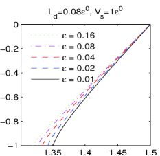
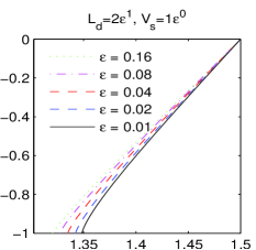
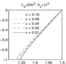
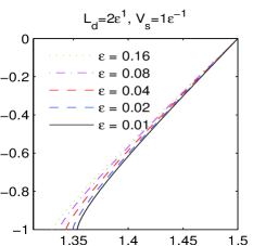
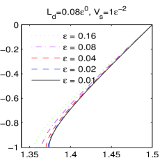
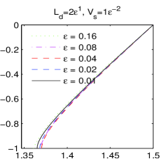
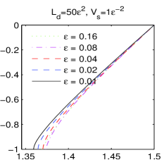
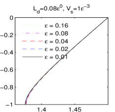
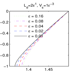
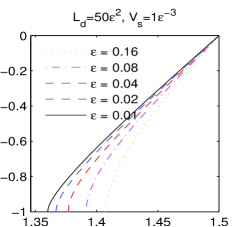
Figure 2: Numerical results at $T=0.2$ with different $\mathsf{L_{d}}$ and $\mathsf{V_{s}}$ values, $\theta_{s}=90^{\circ}$. Since the contact lines are symmetric with respect to point $(1.5,0)$, we only plot the bottom parts to show the convergence.

The left column of Fig. 2 show the results for $\mathsf{L_{d}}=O(1)$ and $\mathsf{V_{s}}=O(\varepsilon^{\beta})$, with $\beta=0,-1,-2,-3$, respectively. It is known that for this case, the Navier-Stokes-Cahn-Hilliard system converges to coupled Navier-Stokes and Hele-Shaw equations (Wang & Wang, 2007). We could also see that the dynamic contact angle approaches to the Young’s angle with increasing relaxation parameter $\mathsf{V_{s}}$. In the largest relaxation parameter $\mathsf{V_{s}}=O(\varepsilon^{-3})$ case, the dynamic contact angle is almost equal to the Young’s angle. We observe that this case exhibits the best convergence rate to a sharp-interface limit. The results are consistent with the numerical observations by Yue, Zhou & Feng (2010). In their experiments, the boundary condition $\mathcal{L}(\phi)=0$ is used, which corresponds to a infinite large parameter $\mathsf{V}_{s}$. They found that the sharp interface limit is obtained only when the mobility parameter is of order $O(1)$.

The middle column of Fig. 2 show the results for $\mathsf{L_{d}}=O(\varepsilon)$ and $\mathsf{V_{s}}=O(\varepsilon^{\beta})$, with $\beta=0,-1,-2,-3$, respectively. For different choice of $\mathsf{V_{s}}$, the sharp-interface limits of the diffuse interface model are slightly different. With increasing relaxation parameter $\mathsf{V_{s}}$ (or decreasing $\beta$), the dynamic contact angle will approach to the stationary contact angle $\theta_{s}=90^{\circ}$. From Fig. 2 (h) and (k), we could see that the dynamic contact angle is almost $90^{\circ}$ for small $\varepsilon$. These results are consistent with the asymptotic analysis in the previous section. More interestingly, the different choices of $\mathsf{V_{s}}$ might also affect the convergence rates. In seems that the convergence rate to the sharp-interface limit for $\mathsf{V_{s}}=O(\varepsilon^{-1})$ is slightly better than other cases. For the case $\mathsf{V_{s}}=O(\varepsilon^{-3})$, the convergence rate seems very slow. This indicates the phase-field model might not convergence for infinite large relaxation parameter when $\mathsf{L_{d}}=O(\varepsilon)$, as shown by Yue, Zhou & Feng (2010).

The right column of Fig. 2 show the results for $\mathsf{L_{d}}=O(\varepsilon^{2})$ and $\mathsf{V_{s}}=O(\varepsilon^{\beta})$, with $\beta=0,-1,-2,-3$, respectively. In this case, the Navier-Stokes-Cahn-Hilliard system still converges to that standard incompressible two-phase Navier-Stokes equations.  Magaletti et al. (2013) considered the case without moving contact lines, found that $\mathsf{L_{d}}=O(\varepsilon^{2})$ give the best convergence rate. Here we show some numerical results for moving contact line problems. In this case, the choice of $\mathsf{V_{s}}=O(\varepsilon^{-1})$ seems correspond to slightly faster convergence rate than other choices. This is similar to the $\mathsf{L_{d}}=O(\varepsilon)$ case.

On the other hand, we observe that when the boundary relaxation $\mathsf{V_{s}}=O(\varepsilon^{\beta})$ with $\beta\geq-1$ (the first and second row of Fig. 2), the boundary diffusion can be considered as small, then the scaling $L_{d}=O(\varepsilon^{2})$ gives the best convergence rate. This is similar to the results of phase-field model without contact lines obtained by Magaletti et al. (2013), where they give an elaborate analysis. On the other hand, when $V_{s}=O(\varepsilon^{\beta})$ with $\beta\leq-2$ (the third and fourth row of Fig. 2), the boundary diffusion is relatively large, then $L_{d}=O(1)$ gives best convergence rate. This is consistent to the finding by Yue, Zhou & Feng (2010). The observation is helpful in the real applications using the GNBC model.

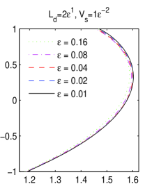
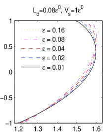
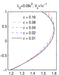
Figure 3: Numerical results at $T=0.2$ with different $\mathsf{L_{d}}$ and $\mathsf{V_{s}}$ values, $\theta_{s}=60^{\circ}$.

We also did experiments for the case when $\theta_{s}=60^{\circ}$. The numerical results are similar to the case when $\theta_{s}=90^{\circ}$. In Fig. 3 we present only a few snapshots of MCLs at $T=0.2$ for the case when $\theta_{s}=60^{\circ}$. Here we focus on the differences between the choices $\mathsf{L_{d}}=O(\varepsilon)$ and $\mathsf{L_{d}}=O(1)$. We show three cases $\mathsf{V_{s}}=O(1)$, $O(\varepsilon^{-1})$ and $O(\varepsilon^{-2})$. From the figure, we could see that the convergence rate for $\mathsf{L_{d}}=O(\varepsilon)$ is better than $\mathsf{L_{d}}=O(1)$ when $\mathsf{V_{s}}$ is $O(1)$ and $O(\varepsilon^{-1})$.

5 Conclusion

We studied the convergence behavior with respect to the Cahn number $\varepsilon$ of a phase field moving contact line model incorporating dynamic contact line condition in different situations, using asymptotic analysis and numerical simulations. In particular, we considered the situations of $\varepsilon$-dependent mobility $\mathsf{L_{d}}$ and boundary relaxation $\mathsf{V_{s}}$. This extends the study by Yue, Zhou & Feng (2010) and Wang & Wang (2007). Yue, Zhou & Feng (2010) showed that $\mathsf{L_{d}}=O(1)$ is the only proper choice for the sharp-interface limit of a diffuse interface model with no slip boundary condition.  Wang & Wang (2007) deduced that the sharp-interface limit of the phase-field model with the GNBC for the case $\mathsf{L_{d}}=O(1)$ obeys a Hele-Shaw flow.

We did asymptotic analysis for the phase-field model with the GNBC for the case $\mathsf{L_{d}}=O(\varepsilon)$. We show that the sharp-interface limit is the incompressible two-phase Navier-Stokes equations with standard jump condition for velocity and stress on the interfaces. We also show that the different choices of the scaling of $\mathsf{V_{s}}$ correspond to different boundary conditions in the sharp-interface limit.

Our numerical results show that when the boundary relaxation $\mathsf{V_{s}}=O(\varepsilon^{\beta})$ with $\beta\geq-1$, the boundary diffusion can be considered as small, the scaling $L_{d}=O(\varepsilon^{\alpha}),\alpha=0,1,2$ all give convergence, but $\alpha=2$ gives the best convergence rate. This is consistent to the results of phase-field model without contact lines obtained by Magaletti et al. (2013). On the other hand, when $V_{s}=O(\varepsilon^{\beta})$ with $\beta\leq-2$, $L(d)=O(\varepsilon^{\alpha}),\alpha=0,1$ will give better convergence rate, while $\alpha=2$ also exhibits convergence. The case $\alpha=0$ give best convergence rate for $\mathsf{V_{s}}$ very large is consistent to the finding by Yue, Zhou & Feng (2010). The larger convergence region of $\alpha$ is due to the fact that the generalized Navier slip boundary condition and the dynamic contact line condition are incorporated in the phase field MCL model we used. Our analysis and numerical studies will be helpful in the real applications using the GNBC model.

Appendix: The numerical scheme

The CHNS system (8)-(9) are solved using a second-order accurate and energy stable time marching scheme basing on invariant energy quadratization skill developed by Yang & Yu (2017). For clarity, we list the details of the scheme below. Let $\delta t>0$ be the time step-size and set $t^{n}=n\delta t$. For any function $S(\mathbf{x},t)$, let $S^{n}$ denotes the numerical approximation to $S(\cdot,t)|_{t=t^{n}}$, and $S_{\star}^{n+1}:=2S^{n}-S^{n-1}$. We introduce $U^{0}=(\phi^{0})^{2}-1$, $W^{0}=\sqrt{\hat{\gamma}_{wf}(\phi^{0})}$, where

$$\hat{\gamma}_{wf}(\phi)=\left\{\begin{array}[]{ll}\frac{\sqrt{2}}{3}-\frac{\sqrt{2}}{6}\cos\theta_{s}(3\phi-\phi^{3}),&\mbox{if}\ |\phi|\leq 1,\\ \frac{\sqrt{2}}{3}-\frac{\sqrt{2}}{3}\cos\theta_{s},&\mbox{otherwise}.\end{array}\right.$$ (69)

Assuming that $(\phi,\mathbf{v},p,U,W)^{n-1}$ and $(\phi,\mathbf{v},p,U,W)^{n}$ are already known, we compute $\phi^{n+1},\mathbf{v}^{n+1}$, $p^{n+1},U^{n+1},W^{n+1}$ in two steps:

Step 1: We update $\phi^{n+1},\tilde{\mathbf{v}}^{n+1},U^{n+1},W^{n+1}$ as follows,

$$\frac{3\phi^{n+1}-4\phi^{n}+\phi^{n-1}}{2\delta t}+\nabla\cdot(\tilde{\mathbf{v}}^{{n+1}}\phi_{\star}^{n+1})=\mathsf{L_{d}}\Delta\mu^{{n+1}},$$ (70)

$$\mu^{{n+1}}=-\varepsilon\Delta\phi^{{n+1}}+\frac{1}{\varepsilon}\phi_{\star}^{n+1}U^{{n+1}},$$ (71)

$$3U^{n+1}-4U^{n}+U^{n-1}=2\phi_{\star}^{n+1}(3\phi^{n+1}-4\phi^{n}+\phi^{n-1}),$$ (72)

$$\mathsf{Re}\Big{[}\frac{3\widetilde{\mathbf{v}}^{n+1}\!\!\!-\!\!4\mathbf{v}^{n}\!+\!\mathbf{v}^{n\!-\!1}}{2\delta t}+B(\mathbf{v}_{\star}^{n+1}\!,\widetilde{\mathbf{v}}^{{n+1}})\!\Big{]}-\!\Delta\widetilde{\mathbf{v}}^{{n+1}}\!\!+\nabla p^{n}\!\!+\mathsf{B}\phi_{\star}^{n+1}\nabla\mu^{{n+1}}=F^{n+1},$$ (73)

with the boundary conditions

$$\widetilde{\mathbf{v}}^{n+1}\cdot{\boldsymbol{n}}=0,$$ (74)

$$\partial_{{\boldsymbol{n}}}\widetilde{\mathbf{v}}_{\tau}^{{n+1}}=-\mathsf{l_{s}}^{-1}(\widetilde{\mathbf{v}}^{{n+1}}-\mathbf{v}_{w})-\frac{1}{\mathsf{V_{s}}}\dot{\phi}^{{n+1}}\nabla_{\tau}\phi_{\star}^{n+1},$$ (75)

$$\partial_{\boldsymbol{n}}\mu^{{n+1}}=0,$$ (76)

$$\varepsilon\partial_{\boldsymbol{n}}\phi^{{n+1}}=-\frac{1}{\mathsf{V_{s}}}\dot{\phi}^{{n+1}}-Z(\phi_{\star}^{n+1})W^{{n+1}},$$ (77)

$$3W^{n+1}-4W^{n}+W^{n-1}=\frac{1}{2}Z(\phi_{\star}^{n+1})(3\phi^{n+1}-4\phi^{n}+\phi^{n-1}),$$ (78)

where

$$B(\mathbf{u},\mathbf{v})=(\mathbf{u}\cdot\nabla)\mathbf{v}+\frac{1}{2}(\nabla\cdot\mathbf{u})\mathbf{v},$$ (79)

$$\dot{\phi}^{{n+1}}=\frac{3\phi^{n+1}-4\phi^{n}+\phi^{n-1}}{2\delta t}+\widetilde{\mathbf{v}}_{\tau}^{{n+1}}\cdot\nabla_{\tau}\phi_{\star}^{n+1},$$ (80)

$$Z(\phi)={\hat{\gamma}^{\prime}_{wf}(\phi)}/\sqrt{\hat{\gamma}_{wf}(\phi)}.$$ (81)

Step 2: We update $\mathbf{v}^{n+1}$ and $p^{n+1}$ as follows,

$$\frac{3\mathsf{Re}}{2\delta t}\big{(}\mathbf{v}^{n+1}-\widetilde{\mathbf{v}}^{n+1}\big{)}+\nabla(p^{n+1}-p^{n})=0,$$ (82)

$$\nabla\cdot\mathbf{v}^{n+1}=0,$$ (83)

with the boundary condition

$$\mathbf{v}^{n+1}\cdot{\boldsymbol{n}}=0\quad\mbox{on}\ \Gamma.$$ (84)

The above scheme are further discretized in space using an efficient Fourier-Legendre spectral method, see (Shen et al., 2015) and (Yu & Yang, 2017) for more details about the spatial discretization and solution procedure. The scheme (70)-(84) can be proved to be unconditional energy stable (Yang & Yu, 2017). But to get accurate numerical results, we have to take time step-size small enough. In all the simulations in this paper we use $\delta t=0.0001$ and the first order scheme proposed by Shen, Yang & Yu (2015) is used to generate the numerical solution at $t=\delta t$ to start up the second order scheme.

References

- Aland & Chen (2015) Aland, Sebastian & Chen, Feng 2015 An efficient and energy stable scheme for a phase-field model for the moving contact line problem. International Journal for Numerical Methods in Fluids .
- Allen & Cahn (1979) Allen, Samuel M & Cahn, John W 1979 A microscopic theory for antiphase boundary motion and its application to antiphase domain coarsening. Acta Metallurgica 27 (6), 1085–1095.
- Anderson et al. (1998) Anderson, Daniel M, McFadden, Geoffrey B & Wheeler, Adam A 1998 Diffuse-interface methods in fluid mechanics. Annual Review of Fluid Mechanics 30 (1), 139–165.
- Bao et al. (2012) Bao, Kai, Shi, Yi, Sun, Shuyu & Wang, Xiao-Ping 2012 A finite element method for the numerical solution of the coupled Cahn-Hilliard and Navier-Stokes system for moving contact line problems. Journal of Computational Physics 231 (24), 8083–8099.
- Blake (2006) Blake, Terence D 2006 The physics of moving wetting lines. Journal of Colloid and Interface Science 299 (1), 1–13.
- Blake & De Coninck (2011) Blake, T. D. & De Coninck, Joël 2011 Dynamics of wetting and kramers’ theory. The European Physical Journal Special Topics 197 (1), 249–264.
- Bonn et al. (2009) Bonn, Daniel, Eggers, Jens, Indekeu, Joseph, Meunier, Jacques & Rolley, Etienne 2009 Wetting and spreading. Reviews of Modern Physics 81 (2), 739.
- Briant et al. (2004) Briant, AJ, Wagner, AJ & Yeomans, JM 2004 Lattice Boltzmann simulations of contact line motion. i. liquid-gas systems. Physical Review E 69 (3), 031602.
- Buscaglia & Ausas (2011) Buscaglia, G. C. & Ausas, R. F. 2011 Variational formulations for surface tension, capillarity and wetting. Computer Methods in Applied Mechanics and Engineering 200 (45), 3011–3025.
- Caginalp & Chen (1998) Caginalp, Gunduz & Chen, Xinfu 1998 Convergence of the phase field model to its sharp interface limits. European Journal of Applied Mathematics 9 (04), 417–445.
- Cahn & Hilliard (1958) Cahn, John W & Hilliard, John E 1958 Free energy of a nonuniform system. i. interfacial free energy. The Journal of Chemical Physics 28 (2), 258–267.
- Carlson et al. (2009) Carlson, Andreas, Do-Quang, Minh & Amberg, Gustav 2009 Modeling of dynamic wetting far from equilibrium. Physics of Fluids 21 (12), 121701.
- Chen et al. (2000) Chen, Hsuan-Yi, Jasnow, David & Viñals, Jorge 2000 Interface and contact line motion in a two phase fluid under shear flow. Physical Review Letters 85 (8), 1686.
- Chen et al. (2014) Chen, Xinfu, Wang, Xiaoping & Xu, Xianmin 2014 Analysis of the Cahn–Hilliard equation with a relaxation boundary condition modeling the contact angle dynamics. Archive for Rational Mechanics and Analysis 213 (1), 1–24.
- Cox (1986) Cox, R. 1986 The dynamics of the spreading of liquids on a solid surface. Part 1. Viscous flow. J. Fluid Mech. 168, 169–194.
- Ding & Spelt (2007) Ding, Hang & Spelt, Peter DM 2007 Wetting condition in diffuse interface simulations of contact line motion. Physical Review E 75 (4), 046708.
- Dussan (1979) Dussan, EB 1979 On the spreading of liquids on solid surfaces: static and dynamic contact lines. Annual Review of Fluid Mechanics 11 (1), 371–400.
- Eggers (2005) Eggers, Jens 2005 Contact line motion for partially wetting fluids. Physical Review E 72 (6), 061605.
- Fakhari & Bolster (2017) Fakhari, Abbas & Bolster, Diogo 2017 Diffuse interface modeling of three-phase contact line dynamics on curved boundaries: A lattice Boltzmann model for large density and viscosity ratios. Journal of Computational Physics 334, 620–638.
- Gao & Wang (2012) Gao, Min & Wang, Xiao-Ping 2012 A gradient stable scheme for a phase field model for the moving contact line problem. Journal of Computational Physics 231 (4), 1372–1386.
- Gao & Wang (2014) Gao, Min & Wang, Xiao-Ping 2014 An efficient scheme for a phase field model for the moving contact line problem with variable density and viscosity. Journal of Computational Physics 272, 704–718.
- Gerbeau & Lelievre (2009) Gerbeau, J-F & Lelievre, Tony 2009 Generalized Navier boundary condition and geometric conservation law for surface tension. Computer Methods in Applied Mechanics and Engineering 198 (5), 644–656.
- Guo et al. (2013) Guo, Shuo, Gao, Min, Xiong, Xiaomin, Wang, Yong Jian, Wang, Xiaoping, Sheng, Ping & Tong, Penger 2013 Direct measurement of friction of a fluctuating contact line. Physical Review Letters 111 (2), 026101.
- Gurtin et al. (1996) Gurtin, Morton E, Polignone, Debra & Vinals, Jorge 1996 Two-phase binary fluids and immiscible fluids described by an order parameter. Mathematical Models and Methods in Applied Sciences 6 (06), 815–831.
- Haley & Miksis (1991) Haley, Patrick J & Miksis, Michael J 1991 The effect of the contact line on droplet spreading. Journal of Fluid Mechanics 223, 57–81.
- Huang et al. (2009) Huang, JJ, Shu, C & Chew, YT 2009 Mobility-dependent bifurcations in capillarity-driven two-phase fluid systems by using a lattice Boltzmann phase-field model. International Journal for Numerical Methods in Fluids 60 (2), 203–225.
- Huh & Scriven (1971) Huh, Chun & Scriven, LE 1971 Hydrodynamic model of steady movement of a solid/liquid/fluid contact line. Journal of Colloid and Interface Science 35 (1), 85–101.
- Jacqmin (1999) Jacqmin, David 1999 Calculation of two-phase Navier–Stokes flows using phase-field modeling. Journal of Computational Physics 155 (1), 96–127.
- Jacqmin (2000) Jacqmin, D. 2000 Contact-line dynamics of a diffuse fluid interface. Journal of Fluid Mechanics 402, 57–88.
- Khatavkar et al. (2006) Khatavkar, VV, Anderson, PD & Meijer, HEH 2006 On scaling of diffuse–interface models. Chemical Engineering Science 61 (8), 2364–2378.
- Kusumaatmaja et al. (2016) Kusumaatmaja, Halim, Hemingway, Ewan J & Fielding, Suzanne M 2016 Moving contact line dynamics: from diffuse to sharp interfaces. Journal of Fluid Mechanics 788, 209–227.
- Lowengrub & Truskinovsky (1998) Lowengrub, J & Truskinovsky, L 1998 Quasi–incompressible Cahn-Hilliard fluids and topological transitions. Proceedings of the Royal Society of London A: Mathematical, Physical and Engineering Sciences 454 (1978), 2617–2654.
- Magaletti et al. (2013) Magaletti, F, Picano, Francesco, Chinappi, M, Marino, Luca & Casciola, Carlo Massimo 2013 The sharp-interface limit of the Cahn-Hilliard/Navier-Stokes model for binary fluids. Journal of Fluid Mechanics 714, 95–126.
- Marmottant & Villermaux (2004) Marmottant, Philippe & Villermaux, Emmanuel 2004 On spray formation. Journal of Fluid Mechanics 498, 73–111.
- Pego (1989) Pego, Robert L 1989 Front migration in the nonlinear Cahn-Hilliard equation. Proc. Royal Soc. London A 422 (1863), 261–278.
- Pismen (2002) Pismen, LM 2002 Mesoscopic hydrodynamics of contact line motion. Colloids and Surfaces A: Physicochemical and Engineering Aspects 206 (1), 11–30.
- Pismen & Pomeau (2000) Pismen, Len M & Pomeau, Yves 2000 Disjoining potential and spreading of thin liquid layers in the diffuse-interface model coupled to hydrodynamics. Physical Review E 62 (2), 2480.
- Qian et al. (2003) Qian, T., Wang, X.-P. & Sheng, P. 2003 Molecular scale contact line hydrodynamics of immiscible flows. Phys. Rev. E 68, 016306.
- Qian et al. (2004) Qian, T., Wang, X.-P. & Sheng, P. 2004 Power-law slip profile of the moving contact line in two-phase immiscible flows. Phys. Rev. lett. 63, 094501.
- Qian et al. (2006) Qian, T., Wang, X.-P. & Sheng, P. 2006 A variational approach to moving contact line hydrodynamics. J. Fluid Mech. 564, 333–360.
- Ren & E (2007) Ren, Weiqing & E, Weinan 2007 Boundary conditions for the moving contact line problem. Physics of Fluids 19 (2), 022101.
- Ren & E (2011) Ren, Weiqing & E, Weinan 2011 Derivation of continuum models for the moving contact line problem based on thermodynamic principles. Commun. Math. Sci 9 (2), 597–606.
- Renardy et al. (2001) Renardy, Michael, Renardy, Yuriko & Li, Jie 2001 Numerical simulation of moving contact line problems using a volume-of-fluid method. Journal of Computational Physics 171 (1), 243–263.
- Reusken et al. (to appear) Reusken, Arnold, Xu, Xianmin & Zhang, Liang to appear Finite element methods for a class of continuum models for immiscible flows with moving contact lines. International Journal for Numerical Methods in Fluids .
- Schwartz & Eley (1998) Schwartz, Leonard W & Eley, Richard R 1998 Simulation of droplet motion on low-energy and heterogeneous surfaces. Journal of Colloid and Interface Science 202 (1), 173–188.
- Seppecher (1996) Seppecher, Pierre 1996 Moving contact lines in the Cahn-Hilliard theory. International Journal of Engineering Science 34 (9), 977–992.
- Seveno et al. (2009) Seveno, David, Vaillant, Alexandre, Rioboo, Romain, Adao, H, Conti, J & De Coninck, Joël 2009 Dynamics of wetting revisited. Langmuir 25 (22), 13034–13044.
- Shen et al. (2015) Shen, Jie, Yang, Xiaofeng & Yu, Haijun 2015 Efficient energy stable numerical schemes for a phase field moving contact line model. Journal of Computational Physics 284, 617–630.
- Shikhmurzaev (1993) Shikhmurzaev, Yu D 1993 The moving contact line on a smooth solid surface. International Journal of Multiphase Flow 19 (4), 589–610.
- Sibley et al. (2013a) Sibley, David N, Nold, Andreas & Kalliadasis, Serafim 2013a Unifying binary fluid diffuse-interface models in the sharp-interface limit. Journal of Fluid Mechanics 736, 5–43.
- Sibley et al. (2013b) Sibley, David N, Nold, Andreas, Savva, Nikos & Kalliadasis, Serafim 2013b The contact line behaviour of solid-liquid-gas diffuse-interface models. Physics of Fluids 25 (9), 092111.
- Sibley et al. (2013c) Sibley, D. N., Nold, A., Savva, N. & Kalliadasis, S. 2013c On the moving contact line singularity: Asymptotics of a diffuse-interface model. Euro. Phys. J. E 36 (3), 1–7.
- Snoeijer & Andreotti (2013) Snoeijer, Jacco H & Andreotti, Bruno 2013 Moving contact lines: scales, regimes, and dynamical transitions. Annual Review of Fluid Mechanics 45, 269–292.
- Spelt (2005) Spelt, Peter DM 2005 A level-set approach for simulations of flows with multiple moving contact lines with hysteresis. Journal of Computational Physics 207 (2), 389–404.
- Sui et al. (2014) Sui, Yi, Ding, Hang & Spelt, Peter DM 2014 Numerical simulations of flows with moving contact lines. Annual Review of Fluid Mechanics 46, 97–119.
- Teigen et al. (2011) Teigen, Knut Erik, Song, Peng, Lowengrub, John & Voigt, Axel 2011 A diffuse-interface method for two-phase flows with soluble surfactants. Journal of Computational Physics 230 (2), 375–393.
- Wang et al. (2008) Wang, X.-P., Qian, T. & Sheng, P. 2008 Moving contact line on chemically patterned surfaces. J. Fluid Mech. 605, 59–78.
- Wang & Wang (2007) Wang, Xiao-Ping & Wang, Ya-Guang 2007 The sharp interface limit of a phase field model for moving contact line problem. Methods and Applications of Analysis 14 (3), 287–294.
- Yamamoto et al. (2014) Yamamoto, Yasufumi, Tokieda, Katsunori, Wakimoto, Tatsuro, Ito, Takahiro & Katoh, Kenji 2014 Modeling of the dynamic wetting behavior in a capillary tube considering the macroscopic–microscopic contact angle relation and generalized Navier boundary condition. International Journal of Multiphase Flow 59, 106–112.
- Yang & Yu (2017) Yang, Xiaofeng & Yu, Haijun 2017 Efficient second order energy stable schemes for a phase-field moving contact line model. submitted .
- Yu & Yang (2017) Yu, Haijun & Yang, Xiaofeng 2017 Numerical approximations for a phase-field moving contact line model with variable densities and viscosities. Journal of Computational Physics 334, 665–686.
- Yue & Feng (2011a) Yue, P. & Feng, J. J. 2011a Can diffuse-interface models quantitatively describe moving contact lines? The European Physical Journal Special Topics 197 (1), 37–46.
- Yue & Feng (2011b) Yue, P. & Feng, J. J. 2011b Wall energy relaxation in the Cahn-Hilliard model for moving contact lines. Physics of Fluids 23, 012106.
- Yue et al. (2004) Yue, Pengtao, Feng, James J, Liu, Chun & Shen, Jie 2004 A diffuse-interface method for simulating two-phase flows of complex fluids. Journal of Fluid Mechanics 515, 293–317.
- Yue et al. (2010) Yue, P., Zhou, C. & Feng, J. J. 2010 Sharp-interface limit of the Cahn-Hilliard model for moving contact lines. Journal of Fluid Mechanics 645, 279–294.
- Zhou & Sheng (1990) Zhou, Min-Yao & Sheng, Ping 1990 Dynamics of immiscible-fluid displacement in a capillary tube. Physical Review Letters 64 (8), 882.