Generalized Geometric Programming
for Rate Allocation in Consensus

Abstract

Distributed averaging, or distributed average consensus, is a common method for computing the sample mean of the data dispersed among the nodes of a network in a decentralized manner. By iteratively exchanging messages with neighbors, the nodes of the network can converge to an agreement on the sample mean of their initial states. In real-world scenarios, these messages are subject to bandwidth and power constraints, which motivates the design of a lossy compression strategy. Few prior works consider the rate allocation problem from the perspective of constrained optimization, which provides a principled method for the design of lossy compression schemes, allows for the relaxation of certain assumptions, and offers performance guarantees. We show for Gaussian-distributed initial states with entropy-coded scalar quantization and vector quantization that the coding rates for distributed averaging can be optimized through generalized geometric programming. In the absence of side information from past states, this approach finds a rate allocation over nodes and iterations that minimizes the aggregate coding rate required to achieve a target mean square error within a finite run time. Our rate allocation is compared to some of the prior art through numerical simulations. The results motivate the incorporation of side-information through differential or predictive coding to improve rate-distortion performance.

I Introduction

The proliferation of wireless sensors and large distributed data sets in recent years has provided significant motivation for the development of distributed computing methods. In many distributed computing settings, it is necessary to compute a function of data that may be dispersed among a number of computing nodes. Examples include wireless sensor networks (WSNs), where each agent observes a different measurement of a physical process, and large-scale server farms, where the size of the data set requires distributed storage [1]. The class of distributed algorithms considered in this paper computes these functions using only interactions among local subsets of the network nodes. One popular approach to distributed function computation, which has many variants, is consensus [2, 3]. Consensus has found applications in a wide variety of settings, including distributed swarm control, sensor fusion, optimization, filtering, environmental monitoring, and distributed learning [2, 4, 5].

As a motivating example for our lossy compression framework, we consider the application of distributed averaging in representation learning for the internet of things (IoT). Distributed average consensus helps different nodes share intermediate results within a distributed version of the power method [6], which can be used in distributed dictionary learning schemes such as cloud K-SVD [5]. Take face recognition as an example. Powered by IoT, a camera network can gather a large number of face images and train a face recognition model using dictionary learning [7]. If these cameras can share the data they gathered and re-train their face recognition model, then they can improve their performance over time. In fully connected networks, the cameras would easily share newly gathered images and re-train their face recognition model efficiently. However, in IoT, the network is often ad-hoc and may have sparse connectivity. Furthermore, in dictionary learning for images, large quantities of data must be communicated among nodes, which strains the energy constraints of IoT devices [8].

In this work, we propose a scheme that offers the potential to balance the competing metrics of communication load, estimation error, and execution time for such IoT applications. After running for a finite number of iterations $T<\infty$, average consensus will produce an estimate of the mean that has some associated mean square error (MSE), ${\mathrm{MSE}}(T)>0$. If the internode messages are quantized, this process will require the transmission of a total or aggregate coding rate, $R_{\text{agg}}>0$. Our goal is to minimize the communication load, measured by $R_{\text{agg}}$, subject to a given number of iterations to be carried out ($T$) and a desired final accuracy, ${\mathrm{MSE}}(T)$. To perform this minimization, we use the theory of generalized geometric programming (GGP) [9, 10] to formulate a convex program that can find the global optimum solution for certain lossy compression schemes.

I-A Prior art

Many early works on consensus assumed that the nodes could communicate real-valued data to one another [11]. In realistic scenarios, the nodes must communicate within bandwidth and energy constraints, which can have a significant impact on the convergence of distributed averaging algorithms. Although many papers have been published on quantized consensus in recent years (e.g., [12, 13, 14, 15, 11, 16, 1, 4, 17]), a large portion considers trade-offs among run time, communication load, and final accuracy without formulating the problem as constrained optimization. Early publications on quantized consensus (e.g., [19, 11]) show that introducing perturbations of constant variance (such as quantization error) into the traditional consensus state update prevents convergence due to the limited precision of the quantizer. Due to the difficulties associated with quantization error, many works (e.g., [12, 20, 21, 13, 15, 14]) address the incorporation of dynamic coding strategies into consensus protocols. However, few prior schemes explicitly consider the rate-distortion (RD) trade-off, and they instead offer heuristics to optimize their respective performance metrics.

Several papers (e.g., [12, 20, 21]) consider the possibility of using differential coding (also called difference quantization) [22] with a shrinking quantization range during the transmission of messages between nodes. Of these, Thanou et al. [13] demonstrated lower MSE than previous works in this area (e.g., [20, 12]) with equal communication load. Although these papers [13, 20, 12] exploit side-information in their coding strategies, they study the simple fixed-rate uniform quantizer and do not make effective use of lossy compression to balance the trade-offs among $T$, ${\mathrm{MSE}}(T)$, and $R_{\text{agg}}$.

Yildiz and Scaglione [15, 14], unlike other authors, explicitly considered the RD trade-off to achieve an asymptotic MSE value in consensus for the case of Gaussian initial states. They proposed schemes based on differential [15], predictive, and Wyner-Ziv coding [14]. Despite their sophisticated coding approaches, the state update step they used can only provide bounded steady-state error in the limit of many consensus iterations, so that $\lim_{T\rightarrow\infty}{\mathrm{MSE}}(T)>0$ [14].

In addition to these dynamic coding strategies [20, 12, 13, 14], a few works [4, 17] consider optimization strategies for energy consumption in wireless sensor networks. However, Nokleby et al. [4] require a specific topological evolution of the network. Huang and Hua [17] keep the coding rates for their fixed-rate uniform quantizers constant across both nodes and iterations, which does not fully explore the more general space of node- and time-varying rates.

A handful of works (e.g., [23, 24, 25, 26]) analyze consensus from the viewpoint of information theory. Yang et al. [26] considered RD bounds for data aggregation, in which data is routed through a tree network to a fusion center, and consensus, in which each node forms an estimate of the desired quantity. Although Yang et al. [26] provided bounds on the RD relationship for consensus in trees and proved the achievability of the derived bounds, their analysis is limited to the setting where the network is tree structured. Often it is beneficial to consider more flexible topologies, such as random geometric graphs, which have been used to model WSNs [27]. In general, random geometric graphs and their real-world WSN counterparts have loops.

I-B Our contributions

This paper presents a framework for attaining an estimate of the network sample mean at each node, within a desired average level of accuracy, with finite run time and minimal total communication cost (measured by $R_{\text{agg}}$) using either deterministic or dithered quantization. Our framework is informed by the results of RD theory [28] and convex optimization [9]. In the plethora of literature we surveyed, a crucial problem that has not been addressed is the optimization of quantization schemes for finite run-time without a certain set of limiting assumptions. Prior works restrict the topology to trees [26], assume a certain form for the rate/distortion sequences [14, 15], restrict the rates to be the same at each node and/or iteration [17, 13, 15], or use bounds on the MSE or asymptotic MSE values, rather than exact MSE quantities [17, 15], in their analyses. The key contribution of this work is the use of GGP [10] to minimize the communication load subject to an accuracy constraint, which avoids the previously discussed restrictions. The advantages of our approach are (i) ignorance about the parametric form of the allocated rates, which avoids the introduction of unjustified or unnecessary assumptions; (ii) support for different rates at each node and iteration of distributed average consensus; and (iii) optimization with respect to exact MSE constraints (rather than bounds) for finite iteration count.

I-C Notation

We denote the positive-valued subset of a set $\mathcal{S}$ by $\mathcal{S}_{>0}$ and the nonnegative-valued subset by $\mathcal{S}_{\geq 0}$. The integers are denoted by $\mathbb{Z}$, and the real numbers by ${\mathbb{R}}$. Vectors are written in boldface lowercase letters (e.g., $\mathbf{x}$). Matrices are written in boldface capital letters (e.g., $\mathbf{A}$). The $(i,j){\text{th}}$ element of matrix ${\mathbf{A}}$ is written $\left[{\mathbf{A}}\right]_{ij}$. Quantities that vary with time are written as functions of time (e.g., $x(t)$). The $\ell_{p}$-norm is written $\lVert\cdot\rVert_{p}$, matrix transpose is written $\{\cdot\}^{\top}$, and matrix inverse is written $\{\cdot\}^{-1}$. The expectation operator is written as ${\mathbb{E}\left[\cdot\right]}$, the mean of a time-dependent random variable ${\mathbf{x}}(t)$ is written $\boldsymbol{\mu}_{{\mathbf{x}}}(t)$, and its covariance is denoted by ${\boldsymbol{\Sigma}_{{\mathbf{x}}}(t)}$. The Kronecker product of two matrices ${\mathbf{A}},\mathbf{B}$ is written ${\mathbf{A}}\otimes\mathbf{B}$. A diagonal matrix is compactly specified as

$$\operatorname{diag}\begin{bmatrix}x_{1}\\ \vdots\\ x_{n}\end{bmatrix}=\begin{bmatrix}x_{1}&\cdots&0\\ \vdots&\ddots&\vdots\\ 0&\cdots&x_{n}\end{bmatrix}.$$ (1)

II Problem formulation

II-A System model

In this paper, communication links are bidirectional, and we model the network as an undirected graph, $\mathcal{G}=\{\mathcal{V},\mathcal{E}\}$, comprised of a set of $m$ vertices (nodes) $\mathcal{V}$ and a set of edges $\mathcal{E}$ between pairs of vertices [29]. Because the communication links are bidirectional, each edge $(i,j)\in\mathcal{E}$ is represented as an unordered pair of vertices, $i,j\in\mathcal{V}$ [30].

In the simplest case of the consensus problem, each node $i\in\{1,\ldots,m\}$ has an initial scalar quantity $z_{i}(0)\in{\mathbb{R}}$, and the goal is to have all nodes of the network agree upon the sample mean of these quantities by iteratively exchanging messages with their neighbors [30]. The quantities $z_{i}(t)$, $t\geq 0$, will be referred to as “states,” which in this paper are assumed to be real-valued scalar random variables (RVs) with joint Gaussian distribution for $t=0$. More formally, let the (discrete) iteration index be a nonnegative integer, $t\in\mathbb{Z}_{\geq 0}$. At $t=0$, the states $\{z_{i}(t)\}_{i=1}^{m}$ are the initial values to be averaged by the consensus algorithm. For $t\geq 1$, the state $z_{i}(t)$ represents the estimate of the sample average $\widebar{z}:=\frac{1}{m}\sum_{i=1}^{m}z_{i}(0)$ at node $i$. The objective of consensus is for the state $z_{i}(t)$ to eventually equal the sample mean of the initial states: $\lim_{t\rightarrow\infty}z_{i}(t)=\widebar{z}$, $\forall i\in\{1,\ldots,m\}$ [30]. In this paper, we restrict our attention to deterministic, synchronous-update consensus algorithms. We assume the following: (i) the communication link topology of the network is fixed and does not change with time; (ii) at each iteration, every node exchanges messages with only its neighbors; (iii) communication channels are noiseless; (iv) initial states of all nodes are Gaussian with a known joint distribution; (v) each node can use a different rate at each consensus iteration; (vi) internode messages are broadcast to all neighbors at once; and (vii) states are stored with infinite precision, but communicated with limited precision. The last point is well-motivated for nodes with 32- or 64-bit floating-point support.

Given the above assumptions on communication, one popular algorithm for consensus relies on linear updates [30, 2]. Each node updates its state by forming a weighted sum of its own state with those of its neighbors [30],

$$z_{i}(t+1) =w_{ii}z_{i}(t)+\sum_{j\in\mathcal{N}_{i}}w_{ij}z_{j}(t),$$ (2)

where $w_{ij}>0$, $\forall i,j$, $\sum_{k=1}^{m}w_{ik}$ $=\sum_{k=1}^{m}w_{kj}$ $=1$, and $\mathcal{N}_{i}=\{j|(i,j)\in\mathcal{E}\}$ denotes the neighborhood of node $i$. The weights $w_{ij}$ are designed such that $\lim_{t\rightarrow\infty}z_{i}(t)=\widebar{z}$ [30]. The above update equation (2) can be written as [30]

$${{\bf z}(t+1)}={{\bf W}}{{\bf z}(t)}.$$ (3)

The asymptotic convergence condition is then $\lim_{t\rightarrow\infty}{{\bf z}(t)}=\frac{1}{m}{\mathbf{1}}{\mathbf{1}}^{\top}{{\bf z}(0)}=\widebar{z}\,{\mathbf{1}}$. The interested reader is referred to Xiao and Boyd [30] for a study of weight matrix design.

When quantization error is present within the internode messages, the simple linear iteration (3) is not guaranteed to converge [19]. Instead, we use the modified iteration used by Frasca et al. [11], which allows the sample average to be preserved in the presence of quantization errors.

Let $Q:{\mathbb{R}}^{m}\to\mathcal{X}^{m}$ represent quantization to a finite set of representation levels $\mathcal{X}^{m}\subset{\mathbb{R}}^{m}$ (i.e., ${Q({{\bf z}(t)})}=[Q_{1}({z_{1}(t)}),\ldots,Q_{m}({z_{m}(t)})]^{\top}$). The associated quantization error is given by $\boldsymbol{\epsilon}(t):={Q({{\bf z}(t)})}-{{\bf z}(t)}$. We define the distortion at node $i$ and iteration $t$ as $D_{i}(t):={\mathbb{E}\left[\epsilon_{i}^{2}(t)\right]}$. The subscripts on $Q$ indicate that each node can use a different quantizer in general. To allow the algorithm to converge to zero steady-state estimation error, we use the update proposed by Frasca et al. [11], which is

$${{\bf z}(t+1)} ={{\bf z}(t)}+\left({{\bf W}}-{\bf I}\right){Q({{\bf z}(t)})},$$ (4)

where ${\bf I}$ is the identity matrix. The key advantage of this update is that the average $\frac{1}{m}\sum_{i=1}^{m}z_{i}(t)$ of the states $z_{i}(t)$ is preserved at each step $t$, despite quantization error [11]. Because the average is preserved at each iteration, the estimation error from the average consensus state $\widebar{z}{\mathbf{1}}$ is [11]

$${{{\mathbf{e}}(t)}}={\left({\bf I}-{m^{-1}{{\mathbf{1}}{\mathbf{1}}^{\top}}}\right)}{{\bf z}(t)}.$$ (5)

The MSE at node $i$ corresponding to an estimation error ${{{\mathbf{e}}(t)}}$ at iteration $t$ is given by

$$\text{MSE}_{i}(\mathbf{d},t):={\mathbb{E}\left[e_{i}^{2}(t)\right]},$$ (6)

where $\mathbf{d}$ is a vector of all distortions introduced by all nodes throughout the consensus process. The average MSE across the network at the end of iteration $t$ is given by

$$\text{MSE}(t):=\frac{1}{m}\sum_{i=1}^{m}\text{MSE}_{i}(t).$$ (7)

The communication cost of consensus becomes substantial when nodes exchange vector states $\mathbf{z}_{i}(t)\in{\mathbb{R}}^{n}$, rather than scalars. In this case, all entries can be collected into a vector ${\boldsymbol{\zeta}(t)}:=\left[\mathbf{z}^{\top}_{1}(t),\cdots,\mathbf{z}^{\top}_{m}(t)\right]^{\top}\in{\mathbb{R}}^{mn},$ and a matrix is defined $\boldsymbol{\Omega}:={{\bf W}}\otimes{\bf I}_{n}\in{\mathbb{R}}^{mn\times mn}$ [17], so that (4) becomes

$${\boldsymbol{\zeta}(t+1)}={\boldsymbol{\zeta}(t)}+\left({\boldsymbol{\Omega}}-{\bf I}_{mn}\right)Q\left({\boldsymbol{\zeta}(t)}\right).$$ (8)

This work assumes that ${\boldsymbol{\zeta}(t)}$ has a known joint Gaussian distribution, and that the $\mathbf{z}_{i}(t)$ are distributed such that $\boldsymbol{\mu}_{\mathbf{z}_{i}(t)}=\mu_{\mathbf{z}_{i}(t)}{\mathbf{1}}$, and the diagonal of ${\boldsymbol{\Sigma}_{\mathbf{z}_{i}}(t)}$ is $\sigma_{i}^{2}(t){\mathbf{1}}$. This means that the marginal mean and variance can be extracted from any of the elements corresponding to $\mathbf{z}_{i}(t)$ from the joint mean $\boldsymbol{\mu}_{\boldsymbol{\zeta}}(t)$ and joint covariance ${\boldsymbol{\Sigma}_{\boldsymbol{\zeta}}(t)}$, respectively. The marginal means and variances can thus be derived in our case from (4), without considering the higher-dimensional (8). The following statistical analysis will focus on this scalar case.

II-B Main objective

At every iteration $t\in\{0,\ldots,T-1\}$ (where $T$ is the total number of iterations) of the consensus process, each node $i\in\{1,\ldots,m\}$ uses a rate $R_{i}(t)$ to encode its state for transmission to neighboring nodes. This rate is the average number of bits used per symbol. That is, if node $i$ sends a length-$l_{i}(t)$ binary encoding of its scalar state $z_{i}(t)$ to node $j$, then the corresponding rate is given by $R_{i}(t)={\mathbb{E}\left[l_{i}(t)\right]}$, where the expectation is taken over the distribution of $z_{i}(t)$. In general, $R_{i}(t)$ can vary across both nodes and iterations, so that it is not necessary that $R_{i}(t)=R_{j}(s)$ for any $i\neq j,t\neq s$. We simplify notation by defining the rate vector

$${\mathbf{r}}\!:=\!\left[R_{1}(0),...,\!R_{m}(0),...,\!R_{1}(T\!-\!1),...,\!R_{m}(T\!-\!1)\right]^{\top}\!\!\!\!.$$ (9)

Denote the distortions per entry, $D_{i}(t):={\mathbb{E}\left[\epsilon_{i}^{2}(t)\right]}$, incurred using rates ${\mathbf{r}}$ by the distortion vector

$$\mathbf{d}\!:=\!\left[D_{1}(0),...,\!D_{m}(0),...,\!D_{1}(T\!-\!1),...,\!D_{m}(T\!-\!1)\right]^{\top}\!\!\!\!.$$ (10)

One key quantity we use to determine the cost of running the consensus process is the aggregate coding rate [31, 32]:

$$R_{\text{agg}}:=\sum_{t=0}^{T-1}\sum_{i=1}^{m}R_{i}(t),$$ (11)

which represents the total rate used over the $T$ iterations of the consensus algorithm by all $m$ nodes of the network.

Our main objective is to derive minimization strategies for

$$C({\mathbf{r}},T):=R_{\text{agg}}$$ (12)

for fixed- and variable-length codes for Gaussian-distributed sources using a variety of quantizers.

To efficiently encode the data stored across the network, it is necessary to know the distribution of $z_{i}(t)$ for all $i\in\{1,\ldots,m\}$ and $t\geq 0$. To determine these distributions from (4) and the distributions of the initial states $\{z_{i}(0)\}_{i=1}^{m}$ is difficult in general. Instead, we propose an optimization scheme for entropy-coded uniform scalar quantization (ECSQ) [22] of stationary Gaussian states and RD-optimal vector quantization (VQ) [28] of memoryless Gaussian-distributed states. Because (4) consists of a linear combination of jointly Gaussian RVs and independent quantization errors, it can be proven that the states will remain Gaussian for all $t\geq 0$ [18], and thus the mean and covariance of ${{\bf z}(t)}$ are sufficient to describe its distribution.

It can be shown that, for additive quantization noise and symmetric weight matrices [18]:

$$\boldsymbol{\mu}_{\mathbf{z}}(t+1)={{\bf W}}\boldsymbol{\mu}_{\mathbf{z}}(t),$$ (13)

$$\boldsymbol{\mu}_{\mathbf{e}}(t+1)={\left({\bf I}-{m^{-1}{{\mathbf{1}}{\mathbf{1}}^{\top}}}\right)}{{\bf W}}\boldsymbol{\mu}_{\mathbf{e}}(t),$$ (14)

$${\boldsymbol{\Sigma}_{\mathbf{z}}(t+1)} ={{\bf W}}{\boldsymbol{\Sigma}_{\mathbf{z}}(t)}{{\bf W}}+{\left({{\bf W}}-{\bf I}\right)}{\boldsymbol{\Sigma}_{\boldsymbol{\epsilon}}(t)}{\left({{\bf W}}-{\bf I}\right)},$$ (15)

$${\boldsymbol{\Sigma}_{\mathbf{e}}(t)}={\left({\bf I}-{m^{-1}{{\mathbf{1}}{\mathbf{1}}^{\top}}}\right)}{\boldsymbol{\Sigma}_{\mathbf{z}}(t)}{\left({\bf I}-{m^{-1}{{\mathbf{1}}{\mathbf{1}}^{\top}}}\right)},$$ (16)

where $\mathbf{e}(t)$ is the estimation error (5) and the covariance ${\boldsymbol{\Sigma}_{\boldsymbol{\epsilon}}(t)}$ is diagonal, ${\boldsymbol{\Sigma}_{\boldsymbol{\epsilon}}(t)}=\operatorname{diag}[D_{1}(t),\cdots,D_{m}(t)]^{\top}$. Using these definitions, we present the following mathematical relationships, which we term the state evolution equations. These equations allow us to perform the optimization of the rate vector ${\mathbf{r}}$ using the cost function (12). The marginal source variance ${\nu_{i}(\mathbf{d},t)}$ at node $i$ and iteration $t$ is given by

$${\nu_{i}(\mathbf{d},t)} =\left[{\boldsymbol{\Sigma}_{\mathbf{z}}(t)}\right]_{ii},$$ (17)

the MSE at node $i$ and iteration $t$ is given by

$$\mathrm{MSE}_{i}(\mathbf{d},t) =\left[{\boldsymbol{\Sigma}_{\mathbf{e}}(t)}+\boldsymbol{\mu}_{\mathbf{e}}(t)\boldsymbol{\mu}_{\mathbf{e}}^{\top}(t)\right]_{ii},$$ (18)

and the average MSE across the network at iteration $t$ is

$${\mathrm{MSE}}(\mathbf{d},t) =\frac{1}{m}{\mathrm{tr}}\left({\boldsymbol{\Sigma}_{\mathbf{e}}(t)}+\boldsymbol{\mu}_{\mathbf{e}}(t)\boldsymbol{\mu}_{\mathbf{e}}^{\top}(t)\right),$$ (19)

where ${\mathrm{tr}}\left(\cdot\right)$ denotes the trace of a matrix.

II-C Rate-distortion theory

For encoders operating on real-valued sources, the quantization process necessarily introduces a certain expected distortion $D$ into their representation of the input signal [22]. This distortion can be quantified using a number of metrics, but for the purpose of this paper, we use the square error

$$\delta({{\bf z}(t)},\hat{\mathbf{z}}(t))=\lVert{{\bf z}(t)}-\hat{\mathbf{z}}(t)\rVert_{2}^{2},$$ (20)

so that the expected distortion per node per dimension is given by $D=\frac{1}{m}{\mathbb{E}\left[\lVert{{\bf z}(t)}-\hat{\mathbf{z}}(t)\rVert_{2}^{2}\right]}$ [22]. In general, using a higher coding rate $R$ results in a lower distortion $D$, with the drawback of greater communication load. RD theory [28] quantifies the best possible trade-off between coding rate and distortion. The minimum coding rate $R$ required for any compression scheme to produce an expected distortion less than or equal to a particular value $D$ is given by the RD function $R(D)$ [28].

III Rate allocation via GGP

The key insight of this work is the ability to pose the optimization of the rate vector ${\mathbf{r}}$ as a GGP, for which the global optimum can be found [10]. The resulting scheme finds an efficient rate vector ${\mathbf{r}}$ that achieves a target value of ${\mathrm{MSE}}(\mathbf{d},T)$, given by (19).

When a particular quantizer is used in our problem, it will often have an RD performance trade-off that differs from $R(D)$, which is a bound on the best possible performance [22]. In this paper, we term such a trade-off curve for a particular practical quantizer an operational RD relationship.

For ECSQ and uniform quantization followed by fixed-rate coding in the case of Gaussian sources, the operational RD relationship in the high-rate regime is

$$R(D)\approx\begin{cases}\dfrac{1}{2}\log_{2}\left(\dfrac{\sigma^{2}}{D}\right)+R_{c},\,\,&D\in(0,\sigma^{2}D_{\text{max}}]\\ 0,\,\,&\text{otherwise}\end{cases},$$ (21)

where $\sigma^{2}$ represents the variance of the data to be encoded, and $R_{c}$ and $D_{\text{max}}$ are constants [33]. In some cases, such as infinite-dimensional VQ with memoryless Gaussian sources and dithered [34] scalar uniform quantization [35], the relationship (21) holds for all rates.

The source variance ${\nu_{i}(\mathbf{d},t)}$ is a function of the initial state vector covariance ${\boldsymbol{\Sigma}_{\mathbf{z}}(0)}$ (see (15)) and the distortion vector $\mathbf{d}$ in (10); it evolves as described by (15). The operational RD relationship at all nodes $i\in\{1,\ldots,m\}$ and iterations $t\in\{0,\ldots,T-1\}$ can be expressed as

$$R_{i}(\mathbf{d},t) =\frac{1}{2}\log_{2}\left(\max\left\{\frac{{\nu_{i}(\mathbf{d},t)}}{{D_{i}(t)}},2^{-2R_{c}}\right\}\right)+R_{c}.$$ (22)

The $\max$ in (22) encapsulates the saturation of the RD relationship at $R=0$ in (21). Given $T$ iterations, the goal is to minimize the aggregate coding rate (11), subject to a constraint on the final MSE, ${\mathrm{MSE}}(\mathbf{d},T)\leq\text{MSE}^{*}$ (19). For a target MSE of ${\rm{MSE}}^{*}$, the minimum number of iterations required to achieve that MSE, $T_{\text{min}}=\operatorname*{arg\,min}_{T}\left\{T\,\,|\,\,{\mathrm{MSE}}(\mathbf{d},T)<{\rm{MSE}}^{*},\mathbf{d}=\mathbf{0}\right\}$, can be readily obtained using the state-evolution equations eqs. 13, 14, 15 and 16. More formally, using the operational RD relationship (22), the optimization problem is

$$\underset{\mathbf{d}}{\text{minimize}}\sum_{t=0}^{T-1}\sum_{i=1}^{m}\frac{1}{2}\log_{2}\left(\max\left\{\frac{{\nu_{i}(\mathbf{d},t)}}{{D_{i}(t)}},2^{-2R_{c}}\right\}\right)+R_{c},$$ (23)

subject to the constraints

$${\mathrm{MSE}}(\mathbf{d},T)\leq\text{MSE}^{*},$$ (24)

$${D_{i}(t)}>0,\,\,\,\,\forall i,t.$$ (25)

Note that the above optimization is equivalent to

$$\underset{\mathbf{d}}{\text{minimize}} \ln\left(\prod_{t=0}^{T-1}\prod_{i=1}^{m}\max\left\{\frac{{\nu_{i}(\mathbf{d},t)}}{{D_{i}(t)}},2^{-2R_{c}}\right\}\right),$$ (26)

subject to $$\hskip 54.0pt\text{\eqref{eq:constone}~{}and~{}\eqref{eq:consttwo}}.$$

We will now introduce the concept of GGP and show that the optimization (LABEL:eq:cfun) reduces to such a problem.

III-A Basics of GGP

The following information can be found in Boyd and Vandenberghe [9]. For this subsection, we stay close to the authors’ original notation. In the language of geometric programming, a function of the form

$$f(x)=cx_{1}^{a_{1}}x_{2}^{a_{2}}\cdots x_{n}^{a_{n}},\,\,c>0,\,\,x_{i}>0,\,\,a_{i}\in{\mathbb{R}},\,\,\forall i,$$ (27)

is called a monomial [9, 10]. Similarly, a function of the form

$$f(x)=\sum_{i=1}^{k}g_{i}(x_{1},\ldots,x_{n}),$$ (28)

is a posynomial [9, 10], where $g_{i}(x_{1},\ldots,x_{n})$ are monomials. Generalized posynomials are functions formed from posynomials by operations including addition, multiplication, and maximum [10].

[capbesideposition=right,top, capbesidewidth=44mm]figure[]   

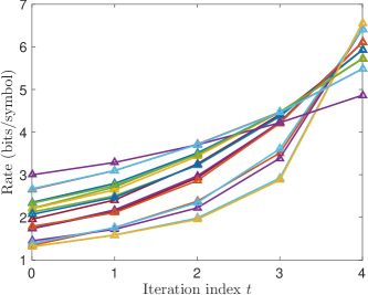
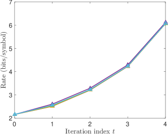
Figure 1: Optimal rates and MSE sequences from the solution of (LABEL:eq:cfun-final) ($T=5$, $\rho_{c}=0.35$, $\sigma_{x}^{2}=1$, $\sigma_{n}^{2}=0.5$, $m=20$). Left: Optimal rate sequences for (LABEL:eq:cfun-final). Right: Optimal rate sequences for (LABEL:eq:cfun-mod). The rates are plotted against iteration indices, and each line represents the rates used by a different sensor. Note that because variable-length coding is used [22], the rates can be non-integer-valued.

A standard inequality-constrained GGP has the form

$$\underset{x_{1},\ldots,x_{n}}{\text{minimize}} C(x_{1},\ldots,x_{n}),$$ (29)

subject to $$\,\,f_{i}(x_{1},\ldots,x_{n})\leq 1,\,\,\,\,\forall i\in\{1,\ldots,n_{f}\},$$

$$\,\,g_{i}(x_{1},\ldots,x_{n})=1,\,\,\,\,\forall i\in\{1,\ldots,n_{g}\},$$

$$\,\,x_{i}>0\,\,\forall i\in\{1,\ldots,n\},$$

where the cost $C(x_{1},\ldots,x_{n})$ and all the inequality constraints $f_{i}(x_{1},\ldots,x_{n})$ are generalized posynomials, and all the equality constraints $g_{i}(x_{1},\ldots,x_{n})$ are monomials [10]. Applying some function transformations, GGPs can be cast in convex form and efficiently solved numerically [10].

III-B Generalized posynomial form of cost function

Applying a monotone increasing function to the cost function (LABEL:eq:cfun) results in an equivalent problem to (LABEL:eq:cfun) [9], so we apply the exponential function to obtain

$$\underset{\mathbf{d}}{\text{minimize}} \prod_{t=0}^{T-1}\prod_{i=1}^{m}\max\left\{\frac{{\nu_{i}(\mathbf{d},t)}}{{D_{i}(t)}},2^{-2R_{c}}\right\},$$ (30)

subject to $$\hskip 48.0pt\text{\eqref{eq:constone}~{}and~{}\eqref{eq:consttwo}}.$$

The above optimization problem (LABEL:eq:cfun-final) is a GGP, which is formally shown in Pilgrim [18].

Two aspects of the above optimization (LABEL:eq:cfun-final) should be highlighted. Because the constraints are allowed to be generalized posynomials, one could also optimize with respect to a constraint on the maximum node MSE, for example,

$$\max_{i}\,\,\{\text{MSE}_{i}(\mathbf{d},T)\}_{i=1}^{m}\leq\text{MSE}^{*},$$ (31)

or constraints on each of the node MSE values,

$$\text{MSE}_{i}(\mathbf{d},T)\leq\text{MSE}^{*}_{i},\,\,\forall i\in\{1,\ldots,m\},$$ (32)

where $\text{MSE}_{i}(\mathbf{d},t)$ is defined in (18). Also, in its most general form, the optimization allows each node to use a different rate or distortion. In the interest of designing a distributed protocol (or for computational efficiency), one may wish to constrain the rates or distortions at each node to be the same. The constraint that all distortions be the same is a straightforward modification of (LABEL:eq:cfun-final) and is also a GGP.

III-C Constant distortion simplification

Solving the exact optimization problem (LABEL:eq:cfun-final) naively requires explicit representation of all $mT$ distortions $D_{i}(t)$ and all the coefficients of the log-sum-exp (LSE) model required to compute $\text{MSE}_{i}(\mathbf{d},t)$ and ${\nu_{i}(\mathbf{d},t)}$ from $\mathbf{d}$. The result of this explicit representation is large computational time and memory complexity. In this section, we explore a simplification of (LABEL:eq:cfun-final) to combat these issues.

In practice, as the network grows (specifically, $m>20$ and $T\geq 6$), the memory and time requirements of the optimization (LABEL:eq:cfun-final) seem to grow quickly. If explicit representation of LSE parameters can be avoided, it is possible to apply other convex optimization methods without these scaling issues. To provide a program that is more easily solvable in practice, we constrain the distortions to be equal at each node, which is equivalent to redefining $\mathbf{d}:=\left[D(0),\ldots,D(T-1)\right]^{\top}$. The optimization is then

$$\underset{\mathbf{d}}{\text{minimize}} \prod_{t=0}^{T-1}\prod_{i=1}^{m}\max{\left\{\frac{{\nu_{i}(\mathbf{d},t)}}{D(t)},2^{-2R_{c}}\right\}},$$ (33)

subject to $$\hskip 48.0pt\text{\eqref{eq:constone}~{}and~{}\eqref{eq:consttwo}}.$$

In the following section, the results of solving the simplified problem (LABEL:eq:cfun-mod) are compared to the solutions of the exact program (LABEL:eq:cfun-final) and the prior art [13, 14]. Surprisingly, the above simplified optimization provides competitive results for random geometric networks [38], with significant reduction in memory and run-time requirements. We conclude by noting that in practical implementation, it is anticipated that the optimization (LABEL:eq:cfun-final) will be run offline with a priori knowledge of the network topology and initial state statistics.

IV Numerical experiments

In this section, we present numerical results that provide insight into the optimal rate sequences that result from solving (LABEL:eq:cfun-final). We further compare the performance of the proposed GGP optimizations (LABEL:eq:cfun-final) and (LABEL:eq:cfun-mod) to the prior art [14, 13]. To test the effectiveness of the proposed approach, we used the CVX toolbox [36, 37] to solve (LABEL:eq:cfun-final) and (LABEL:eq:cfun-mod).

[capbesideposition=right,top, capbesidewidth=44mm]figure[]   

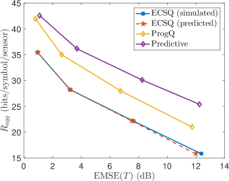
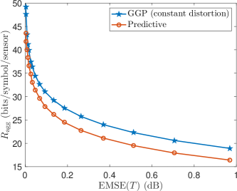
Figure 2: Left: RD trade-off curves for the proposed GGP-optimized ECSQ versus ProgQ [13] and order-one predictive coding [14] ($\rho_{c}=0.45$, $T=7$). Right: Comparison of the proposed GGP-optimization versus order-one predictive for a single realization of the RGG ($\rho_{c}=0.35$, $T=7$), where both schemes use RD-optimal VQ. The corresponding quantization error was simulated by adding white Gaussian noise.

Due to scaling issues, only the fixed-distortion problem (LABEL:eq:cfun-mod) was solved for prior art comparison. The bin size of all fixed-rate uniform quantizers was set to 12 times the standard deviation of the data to prevent clipping.

In the results presented, the networks were generated by random geometric graph (RGG) models [38], and each node state was initialized with the same independent and identically distributed (i.i.d.) variance-$\sigma_{x}^{2}$ zero-mean Gaussian vector ${\mathbf{x}}\in{\mathbb{R}}^{L}$ corrupted by a different variance-$\sigma_{n}^{2}$, zero-mean Gaussian noise $\mathbf{n}_{i}\in{\mathbb{R}}^{L}$, $i\in\{1,\ldots,m\}$. Incorporating noise is important so that the nodes have different estimates of the signal ${\mathbf{x}}$ to average together. The consensus process averages the states elementwise, so this is the same as running $L$ trials of consensus on scalar states $z_{i}(0)$ at once. The random geometric graphs (RGGs) [38] were generated on the unit torus (i.e., edge effects were neglected by “wrapping” edges of $[0,1]^{2}$) [39]. The RGGs provide a model of networks where location determines topology, such as WSNs [40]. An RGG is one for which each node $V_{i}\in\mathcal{V}$ is associated with a coordinate $\mathbf{v}_{i}$. For a given connectivity radius $\rho_{c}$, two nodes $V_{i},V_{j}$ are connected if $\lVert\mathbf{v}_{i}-\mathbf{v}_{j}\rVert_{2}\leq\rho_{c}$ [27].

To better understand the structure of the solutions to the optimization problems (LABEL:eq:cfun-final) and (LABEL:eq:cfun-mod), we present some simulation results. Each of these results is taken from single instantiations of the optimization problem (i.e., they are not averaged over multiple trials).

The optimal rate sequences, $\{R_{i}(t)\}_{t=0}^{T-1}$, $i\in\{1,\ldots,m\}$, for both the variable-distortion (LABEL:eq:cfun-final) and constant-distortion (LABEL:eq:cfun-mod) problems typically exhibit monotonically nondecreasing structure, with an increasing rate of change toward the final iterations. In the constant-distortion case, the rates $R_{i}(t)\approx\frac{1}{2}\log_{2}\left(\max\left\{\frac{{\nu_{i}(\mathbf{d},t)}}{D_{i}(t)},2^{-2R_{c}}\right\}\right)+R_{c}$ are similar because the ratios $\frac{{\nu_{i}(\mathbf{d},t)}}{D_{i}(t)}$ in the Gaussian operational RD relationship (21) are similar across the network. Examples of optimal rate sequences are provided for both variants of the optimization problem LABEL:eq:cfun-final and LABEL:eq:cfun-mod in Fig. 1.

The pattern of these rate sequences is intuitive, and it mirrors the results of Zhu and coauthors’ study of multiprocessor approximate message passing [31, 41, 32]. As the estimate of the sample mean at each node increases in precision, higher-resolution messages must be exchanged among nodes to achieve increasing estimation quality. In the case of coding without side information, this improving precision requires using larger coding rates in the later iterations.

To compare our work to the prior art [14, 13], we generated 32 RGGs [38] with connectivity radius $\rho_{c}\in\{0.35,0.45\}$ on a two-dimensional unit torus. For each of these networks, consensus was run on 1,000 realizations of the initial states, which were length-10,000 i.i.d. Gaussian vectors $\mathbf{z}_{i}(0)={\mathbf{x}}+\mathbf{n}_{i},$ $\forall i\in\{1,\ldots,m\}$, ${\mathbf{x}}\sim\mathcal{N}(\mathbf{0},{\bf I}),\mathbf{n}_{i}\sim\mathcal{N}(\mathbf{0},0.5{\bf I})$. This corresponds to $\text{SNR}:=\frac{\sigma_{x}^{2}}{\sigma_{n}^{2}}=2$, which is 3.01 dB. We simulated ProgQ [13] and order-one predictive coding [14], using initial rates $R_{i}(0)\in\{4,\ldots,7\}$ and $R_{i}(0)\in\{3,\ldots,6\}$, $\forall i$, respectively. The measured final MSE values (18) for these schemes were set as the target values for the GGP.

For all schemes, ${\mathrm{MSE}}(\mathbf{d},T)$ and $R_{\text{agg}}$ were computed. These values were averaged over all 32 realizations of each ($\rho_{c}$, $R_{i}(0)$, $T$) setting, and the resulting averages were plotted against each other. Looking at (15), it seems that the MSE for quantized consensus, where $D_{i}(t)\geq 0,\forall i,t$, is greater than in unquantized consensus, where $D_{i}(t)=0,\forall i,t$.

We therefore introduce two terms to define the MSE performance relative to the ideal, unquantized algorithm. To compensate for the effect of network topology on the MSE, we define the lossless MSE,

$$\text{MSE}_{\text{lossless}}(t):={\mathrm{MSE}}(\mathbf{d},t)\Big{|}_{\mathbf{d}=\mathbf{0}}.$$ (34)

Next, define the final excess MSE (EMSE) as

$$\text{EMSE}(T):=10\log_{10}\frac{\text{MSE}(\mathbf{d},T)}{\text{MSE}_{\text{lossless}}(T)},$$ (35)

which represents the increase in MSE over lossless consensus resulting from distortion. The EMSE was used for the generation of RD trade-off curves.

In the case of very low rates using ECSQ on zero-mean Gaussian sources, all elements decoded at a receiving node would be zeros. To prevent this behavior, the maximum normalized distortion $D_{\text{max}}$ allowed was set such that the recieved elements were nonzero at least 1% of the time.

Because of stability issues with the GGP solvers used, Yildiz and Scaglione’s order-one predictive coding implementation [14], which was provided by the authors, was modified to use fixed-rate uniform quantization but allow for the rate to vary with iteration and node indices. This capability was implemented by running two rate update recursions—one to keep track of the ideal (real-valued) rates given by the quantization noise variance recursion [14], and another to perform the predictive coding using rates that were rounded to the nearest integral value.

V Discussion

To adequately discuss the RD results, we first comment on some properties of each prior art scheme presented. The ProgQ algorithm [13] uses a time- and node-invariant fixed-rate uniform quantizer (i.e., $R_{i}(t)=R$, $\forall i\in\{1,\ldots,m\},t\in\{0,\ldots,T-1\}$), whereas Yildiz and Scaglione [14] allow the use of different rates at each node and iteration.

Thanou et al. [13] use the same state update as ours (4), but Yildiz and Scaglione [14] use a different update that is incapable of truly converging in the presence of quantization error. The final asymptotic MSE for the predictive scheme depends on the sum of distortions, $D_{i}(t),t\in\mathbb{Z}_{\geq 0}$. If these distortions are chosen to form a convergent series, then the MSE will converge to a nonzero, but bounded, value. Because of this limitation, the predictive scheme [14] is heavily dependent on the starting rates, $R_{i}(0)$.

In some cases, such as the bottom right of the ECSQ curve in Fig. 2, the predicted performance and measured performance of ECSQ do not match. Because the ECSQ used in the simulations is not dithered [34], the additive quantization model only holds approximately. As $R_{\text{agg}}$ increases, the performance improves, and better adherence to predicted performance can be accomplished using dithering [34].

The RD performance of the proposed optimization scheme (LABEL:eq:cfun-mod) for ECSQ is compared to the predictive coding scheme of Yildiz and Scaglione [14] and the ProgQ algorithm of Thanou et al. [13] in Fig. 2. For our scheme, the predicted RD performance (as computed by the state evolution equations LABEL:\seeqs) is compared to the actual performance. The distortion (measured by the EMSE) is given by the horizontal axis, and the aggregate rate $R_{\text{agg}}$ by the vertical axis. The predicted performance is denoted by a dashed line, while the simulated performance is represented as a solid line. Alongside our approaches, we plot the RD performance of both of the comparators. A curve closer to the bottom left corner of these figures indicates better performance, meaning lower aggregate rate $R_{\text{agg}}$ to achieve the same EMSE, or lower EMSE for a particular $R_{\text{agg}}$.

The numerical results in the left panel of Fig. 2 suggest that our GGP approach outperforms that of Yildiz and Scaglione and Thanou et al. However, a closer look reveals that much if not all of the gain is due to our using variable rate coding, whereas the implementations for the comparators use fixed rate coding. When we evaluated our approach with fixed rate coding using a heuristic proposed in Pilgrim [18], our results were typically somewhat weaker than the comparators. We attribute the performance advantage of ProgQ [13] and predictive coding [14] to their use of side information from previous iterations.

For a fairer comparison to the predictive approach of Yildiz and Scaglione [14], we also simulated their approach against ours (LABEL:eq:cfun-mod) for RD-optimal vector quantizers, which use variable coding rates. The simulations were run on a single instance of the RGG by varying the initial coding rate of the predictive scheme [14] and setting the resulting $\text{EMSE}(T)$ as the target for the optimization (LABEL:eq:cfun-mod). Because the quantization error of infinite-dimensional lattice quantizers approaches an additive white Gaussian noise process [35], these experiments simulated quantization by adding independent noise of variance $D(t)$ to the states. This plot demonstrates the advantage of predictive quantization on an even playing field by allowing both our approach and the predictive scheme [14] to use variable-rate coding.

The ProgQ scheme [13], unlike predictive coding [14], is capable of converging in the limit due to its different state update strategy. Both ProgQ [13] and predictive coding [14] are capable of using constant or even shrinking coding rates to achieve good performance. It is clear from Fig. 1 that our rates grow with $t$. Therefore, as $T\rightarrow\infty$, we expect that ProgQ will outdo our proposed schemes in all settings, despite our constrained optimization, because it can converge in the limit of large $T$ with constant rates.

VI Conclusion

In conclusion, this paper presented a framework for optimizing the source coding performance of distributed average consensus. The key insight of our approach is the formulation of the problem as a GGP [10]. Our framework allows the problem to be transformed to a convex program [9] and solved for the global optimum. Although we do not incorporate knowledge from past iterations, our numerical results are competitive with prior art that uses more sophisticated side information strategies, which motivates the study of optimization for predictive coding schemes.

In light of the performance gain from predictive coding strategies, we feel that future work should focus on variable rate strategies. Moreover, we aim to optimize the predictive approach of Yildiz and Scaglione using our GGP formulation and the state update (8).

References

- [1] N. Noorshams and M. J. Wainwright, “Non-asymptotic analysis of an optimal algorithm for network-constrained averaging with noisy links,” IEEE J. Sel. Topics Signal Process., vol. 5, no. 4, pp. 833–844, Aug. 2011.
- [2] R. Olfati-Saber, J. A. Fax, and R. M. Murray, “Consensus and cooperation in networked multi-agent systems,” Proc. IEEE, vol. 95, no. 1, pp. 215–233, Jan. 2007.
- [3] A. G. Dimakis, S. Kar, J. M. F. Moura, M. G. Rabbat, and A. Scaglione, “Gossip algorithms for distributed signal processing,” Proc. IEEE, vol. 98, no. 11, pp. 1847–1864, Nov. 2010.
- [4] M. Nokleby, W. U. Bajwa, R. Calderbank, and B. Aazhang, “Toward resource-optimal consensus over the wireless medium,” IEEE J. Sel. Topics Signal Process., vol. 7, no. 2, pp. 284–295, Apr. 2013.
- [5] H. Raja and W. U. Bajwa, “Cloud K-SVD: A collaborative dictionary learning algorithm for big, distributed data,” IEEE Trans. Signal Process., vol. 64, no. 1, pp. 173–188, Jan. 2016.
- [6] A. Scaglione, R. Pagliari, and H. Krim, “The decentralized estimation of the sample covariance,” in Proc. IEEE 42nd Asilomar Conf. Signals, Syst., Comput., Oct. 2008, pp. 1722–1726.
- [7] J. Wright, A. Yang, A. Ganesh, S. Sastry, and Y. Ma, “Robust face recognition via sparse representation,” IEEE Trans. Pattern Anal. Mach. Intell., vol. 31, no. 2, pp. 210–227, Feb. 2009.
- [8] G. J. Pottie and W. J. Kaiser, “Wireless integrated network sensors,” Commun. ACM, vol. 43, no. 5, pp. 51–58, May 2000.
- [9] S. Boyd and L. Vandenberghe, Convex Optimization, Cambridge, UK: Cambridge University Press, 2004.
- [10] S. Boyd, S.-J. Kim, L. Vandenberghe, and A. Hassibi, “A tutorial on geometric programming,” Optimization Eng., vol. 8, no. 67, pp. 67–127, Mar. 2007.
- [11] P. Frasca, R. Carli, F. Fagnani, and S. Zampieri, “Average consensus on networks with quantized communication,” Int. J. Robust Nonlinear Control, vol. 19, no. 16, pp. 1787–1816, Nov. 2008.
- [12] R. Carli, F. Bullo, and S. Zampieri, “Quantized average consensus via dynamic coding/decoding schemes,” Int. J. Robust Nonlinear Control, vol. 20, no. 2, pp. 156–175, May 2009.
- [13] D. Thanou, E. Kokiopoulou, Y. Pu, and P. Frossard, “Distributed average consensus with quantization refinement,” IEEE Trans. Signal Process., vol. 61, no. 1, pp. 194–205, Jan. 2013.
- [14] M. E. Yildiz and A. Scaglione, “Coding with side information for rate-constrained consensus,” IEEE Trans. Signal Process., vol. 56, no. 8, pp. 3753–3764, Aug. 2008.
- [15] M. E. Yildiz and A. Scaglione, “Limiting rate behavior and rate allocation strategies for average consensus problems with bounded convergence,” in Proc. IEEE Int. Conf. Acoust., Speech, Signal Process. (ICASSP), Apr. 2008, pp. 2717–2720.
- [16] R. Rajagopal and M. J. Wainwright, “Network-based consensus averaging with general noisy channels,” IEEE Trans. Signal Process., vol. 59, no. 1, pp. 373–385, Jan. 2011.
- [17] Y. Huang and Y. Hua, “On energy for progressive and consensus estimation in multihop sensor networks,” IEEE Trans. Signal Process., vol. 59, no. 8, pp. 3863–3875, Aug. 2011.
- [18] R. Z. Pilgrim, “Coding rate optimization for distributed average consensus,” M.S. thesis, NC State University, Raleigh, NC, July 2017, Available: http://arxiv.org/abs/1710.01816.
- [19] L. Xiao, S. Boyd, and S.-J. Kim, “Distributed average consensus with least-mean-square deviation,” J. Parallel Distributed Comput., vol. 67, no. 1, pp. 33–46, Jan. 2007.
- [20] T. Li, M. Fu, L. Xie, and J.-F. Zhang, “Distributed consensus with limited communication data rate,” IEEE Trans. Autom. Control, vol. 56, no. 2, pp. 279–292, Feb. 2011.
- [21] F. F. C. Rego, Y. Pu, A. Alessandretti, A. P. Aguiar, and C. N. Jones, “A consensus algorithm for networks with process noise and quantization error,” in Proc. 53rd Allerton Conf. Commun., Control, and Comput., Oct. 2015, pp. 488–495.
- [22] A. Gersho and R. M. Gray, Vector Quantization and Signal Compression, Kluwer, 1993.
- [23] O. Ayaso, D. Shah, and M. A. Dahleh, “Information theoretic bounds for distributed computation over networks of point-to-point channels,” IEEE Trans. Inf. Theory, vol. 56, no. 12, pp. 6020–6039, Dec. 2010.
- [24] A. Xu and M. Raginsky, “A new information-theoretic lower bound for distributed function computation,” in Proc. IEEE Int. Symp. Inform. Theory (ISIT), June 2014, pp. 2227–2231.
- [25] H.-I. Su and A. El Gamal, “Distributed lossy averaging,” IEEE Trans. Inf. Theory, vol. 56, no. 7, pp. 3422–3437, July 2010.
- [26] Y. Yang, P. Grover, and S. Kar, “Rate distortion for lossy in-network linear function computation and consensus: Distortion accumulation and sequential reverse water-filling,” IEEE Trans. Inf. Theory, vol. 63, no. 8, pp. 5179–5206, Aug. 2017.
- [27] S. Boyd, A. Ghosh, B. Prabhakar, and D. Shah, “Mixing times for random walks on geometric random graphs,” in Meeting Algorithm Eng. Experiments/Analytic Algorithmics and Combinatorics, Jan. 2005, pp. 240–249.
- [28] T. M. Cover and J. A. Thomas, Elements of Information Theory, New York, NY: Wiley-Interscience, 1991.
- [29] A. Brandstädt, T. Nishizeki, K. Thulasiraman, and S. Arumugam, Eds., Handbook of Graph Theory, Combinatorial Optimization, and Algorithms, vol. 34 of Chapman and Hall/CRC Computer and Information Science Series, Chapman and Hall/CRC, 2016.
- [30] L. Xiao and S. Boyd, “Fast linear iterations for distributed averaging,” Syst. Control Lett., vol. 53, no. 1, pp. 65–78, Sept. 2004.
- [31] J. Zhu, D. Baron, and A. Beirami, “Optimal trade-offs in multi-processor approximate message passing,” Arxiv preprint arXiv:1601.03790, Nov. 2016.
- [32] J. Zhu, R. Pilgrim, and D. Baron, “An overview of multi-processor approximate message passing,” in Proc. 51st IEEE Conf. Inform. Sci. Syst., Mar. 2017.
- [33] H. Gish and J. Pierce, “Asymptotically efficient quantizing,” IEEE Trans. Inf. Theory, vol. 14, no. 5, pp. 676–683, Sept. 1968.
- [34] S. P. Lipshitz, R. A. Wannamaker, and J. Vanderkooy, “Quantization and dither: A theoretical survey,” J. Audio Eng. Soc., vol. 40, no. 5, pp. 355–375, May 1992.
- [35] R. Zamir and M. Feder, “On lattice quantization noise,” IEEE Trans. Inf. Theory, vol. 42, no. 4, pp. 1152–1159, July 1996.
- [36] M. Grant and S. Boyd, “CVX: MATLAB software for disciplined convex programming, version 2.1,” http://cvxr.com/cvx, Mar. 2014.
- [37] M. Grant and S. Boyd, “Graph implementations for nonsmooth convex programs,” in Recent Advances in Learning and Control, V. Blondel, S. Boyd, and H. Kimura, Eds., Lecture Notes in Control and Information Sciences, pp. 95–110. Springer-Verlag Limited, 2008.
- [38] M. Penrose, Random Geometric Graphs, Oxford University Press, 2003.
- [39] E. W. Weisstein, “Square torus,” 2017, From MathWorld—a Wolfram Web Resource.
- [40] P. Gupta and P. R. Kumar, “The capacity of wireless networks,” IEEE Trans. Inf. Theory, vol. 46, no. 2, pp. 388–404, 2000.
- [41] J. Zhu, A. Beirami, and D. Baron, “Performance trade-offs in multi-processor approximate message passing,” in Proc. IEEE Int. Symp. Inform. Theory (ISIT), July 2016, pp. 680–684.