The geodesic $2$-center problem in a simple polygon

Abstract

The geodesic $k$-center problem in a simple polygon with $n$ vertices consists in the following. Find a set $S$ of $k$ points in the polygon that minimizes the maximum geodesic distance from any point of the polygon to its closest point in $S$. In this paper, we focus on the case where $k=2$ and present an exact algorithm that returns a geodesic $2$-center in $O(n^{2}\log^{2}n)$ time.

1 Introduction

The geodesic $k$-center problem in a simple polygon $P$ with $n$ vertices consists in the following. Find a set $S$ of $k$ points in $P$ that minimizes

$$\max_{p\in P}\min_{s\in S}d(s,p),$$

where $d(x,y)$ is the length of the shortest path between $x$ and $y$ lying in $P$ (also called geodesic distance). The set $S$ is called a $k$-center of $P$. Geometrically, this is equivalent to find $k$ smallest-radius geodesic disks with the same radius whose union contains $P$.

The $2$-dimensional Euclidean $k$-center problem is similar to the geodesic $k$-center problem in a simple polygon $P$. The only difference is that in the Euclidean $k$-center problem, the distance between two points $x$ and $y$ is their Euclidean distance, denoted by $\|x-y\|$. That is, given a set $\mathcal{P}$ of $n$ points in the plane, find a set $S$ of $k$ points in $\mathbb{R}^{2}$ that minimizes

$$\max_{p\in\mathcal{P}}\min_{s\in S}\|p-s\|.$$

Computing a $k$-center of points is a typical problem in clustering. Clustering is the task of partitioning a given set into subsets subject to various objective functions, which have applications in pattern-analysis, decision-making and machine-learning situations including data mining, document retrieval, and pattern classification [13]. The Euclidean $k$-center problem has been studied extensively. The $1$-center of $\mathcal{P}$ coincides with the center of the minimum enclosing circle of $\mathcal{P}$, which can be computed in linear time [16]. Chan showed that the $2$-center problem can be solved in $O(n\log^{2}n\log^{2}\log n)$ deterministic time [6]. The $k$-center problem can be solved in $O(n^{O(\sqrt{k})})$ time [12]. It is NP-hard to approximate the Euclidean $k$-center problem within an approximation factor smaller than 1.822 [10]. Kim and Shin presented an $O(n\log^{3}n\log\log n)$-time algorithm for computing two congruent disks whose union contains a convex $n$-gon [14].

The $1$-center problem has also been studied under the geodesic metric inside a simple polygon. Asano and Toussaint presented the first algorithm for computing the geodesic $1$-center of a simple polygon with $n$ vertices in $O(n^{4}\log n)$ time [4]. In 1989, the running time was improved to $O(n\log n)$ time by Pollack et al. [19]. Their technique can be described as follows. They first triangulate the polygon and find the triangle $T$ that contains the center in $O(n\log n)$ time. Then they subdivide $T$ further and find a region containing the center such that the combinatorial structures of the geodesic paths from each vertex of $P$ to all points in that region are the same. Finally, the problem is reduced to find the lowest point of the upper envelope of a family of distance functions in the region, which can be done in linear time using a technique by Megiddo [17]. Recently, the running time for computing the geodesic $1$-center was improved to linear by Ahn et al. [1, 2], which is optimal. In their paper, instead of triangulating the polygon, they construct a set of $O(n)$ chords. Then they recursively subdivide the polygon into $O(1)$ cells by a constant number of chords and find the cell containing the center. Finally, they obtain a triangle containing the center. In this triangle, they find the lowest point of the upper envelope of a family of functions, which is the geodesic 1-center of the polygon, using an algorithm similar to the one of Megiddo [17].

Surprisingly, there has been no result for the geodesic $k$-center problem for $k>1$, except the one by Vigan [20]. They gave an exact algorithm for computing a geodesic $2$-center in a simple polygon with $n$ vertices, which runs in $O(n^{8}\log n)$ time. The algorithm follows the framework of Kim and Shin [14]. However, the algorithm does not seem to work as it is because of the following reasons. They claim that the decision version of the geodesic $2$-center problem in a simple polygon can be solved using a technique similar to the one by Kim and Shin [14] without providing any detailed argument. They apply parametric search using their decision algorithm, but they do not describe how their parallel algorithm works. The parallel algorithm by Kim and Shin does not seem to extend for this problem.

1.1 Our results

In this paper, we present an $O(n^{2}\log^{2}n)$-time algorithm that solves the geodesic $2$-center problem in a simple polygon with $n$ vertices. The main steps of our algorithm can be described as follows. We first observe that a simple polygon $P$ can always be partitioned into two regions by a geodesic path $\pi(x,y)$ such that

• $x$ and $y$ are two points on the boundary of $P$, and

• the set consisting of the geodesic 1-centers of the two regions of $P$ defined by $\pi(x,y)$ is a geodesic 2-center of $P$.

Then we consider $O(n)$ candidate pairs of edges of $P$, one of which, namely $(e,e^{\prime})$, satisfies $x\in e$ and $y\in e^{\prime}$. We explain how to find these candidate pairs of edges in $O(n^{2}\log n)$ time. Finally, we present an algorithm that computes a $2$-center restricted to such a pair of edges in $O(n\log^{2}n)$ time using parametric search [15] with a decision algorithm and a parallel algorithm.

2 Preliminary

A polygon $P$ is said to be simple if it is bounded by a closed path, and every vertices are distinct and edges intersect only at common endpoints. The polygon $P$ is weakly simple if, for any $\varepsilon>0$, there is a simple polygon $Q$ such that the Fréchet distance between $P$ and $Q$ is at most $\varepsilon$ [7]. The algorithms we use in this paper are designed for simple polygons, but they also work for weakly simple polygons.

The vertices of a simple polygon $P$ with $n$ vertices are labeled $v_{1},\ldots,v_{n}$ in clockwise order along the boundary of $P$. We set $v_{n+k}=v_{k}$ for all $k\geq 1$. An edge whose endpoints are $v_{i}$ and $v_{i+1}$ is denoted by $e_{i}$. For ease of presentation, we make the following general position assumption: no vertex of $P$ is equidistant from two distinct vertices of $P$, which was also assumed in [3]. This assumption can be removed by applying perturbation to the degenerate vertices [9].

For any two points $x$ and $y$ lying inside a (weakly) simple polygon $P$, the geodesic path between $x$ and $y$, denoted by $\pi(x,y)$, is the shortest path inside $P$ between $x$ and $y$. The length of $\pi(x,y)$ is called the geodesic distance between $x$ and $y$, denoted by $d(x,y)$. The geodesic path between any two points in $P$ is unique. The geodesic distance and the geodesic path between $x$ and $y$ can be computed in $O(\log n)$ and $O(\log n+k)$ time, respectively, after an $O(n)$-time preprocessing, where $k$ is the number of vertices on the geodesic path [11]. The vertices of $\pi(x,y)$ excluding $x$ and $y$ are reflex vertices of $P$ and they are called the anchors of $\pi(x,y)$. If $\pi(x,y)$ is a line segment, it has no anchor. In this paper, “distance” refers to geodesic distance unless specified otherwise.

Given a set $X$ of points in $P$ (for instance a polygon or a disk), we use $\partial X$ to denote the boundary of $X$. A set $X\subseteq P$ is geodesically convex if $\pi(x,y)\subset X$ for any two points $x$ and $y$ in $X$. For any two points $u$ and $w$ on $\partial P$, let $C[u,w]$ be the part of $\partial P$ in clockwise order from $u$ to $w$. For $u=w$, let $C[u,w]$ be the vertex $u$. The subpolygon of $P$ bounded by $C[u,w]$ and $\pi(u,w)$ is denoted by $P[u,w]$. Note that $P[u,w]$ may not be simple, but it is always weakly simple. Indeed, consider the set of Euclidean disks centered at points on $\pi(u,w)$ with radius $\varepsilon>0$. There exists a simple polygonal curve connecting $u$ and $w$ that lies in the union of these disks and that does not intersect $C[u,w]$ except at $u$ and $w$. The region bounded by that simple curve and $C[u,w]$ is a simple polygon whose Fréchet distance from $P$ is at most $\varepsilon$.

The radius of $P$, denoted by $r(P)$, is defined as $\max_{p\in P}d(c,p)$, where $c$ is the geodesic $1$-center of $P$. Given two points $\alpha,\beta\in\partial P$, we set $r({\alpha},{\beta})=r(P[\alpha,\beta])$. Notice that $r({\alpha},{x})$ is monotonically increasing as $x$ moves clockwise from $\alpha$ along $\partial P$. Similarly, $r({x},{\alpha})$ is monotonically decreasing as $x$ moves clockwise from $\alpha$ along $\partial P$.

The geodesic disk centered at a point $p\in P$ with radius $r$, denoted by $D_{r}(p)$, is the set of points whose geodesic distances from $p$ are at most $r$. The boundary of a geodesic disk inside $P$ consists of disjoint polygonal chains of $\partial P$ and $O(n)$ circular arcs [5]. Given a center $p\in P$ and a radius $r\in\mathbb{R}$, $D_{r}(p)$ can be computed in $O(n)$ time as follows. We first compute the shortest path map of $p$ in linear time [11]. Each cell in the shortest path map of $p$ is a triangle and every point $q$ in the same cell has the same combinatorial structure of $\pi(p,q)$. Thus, a cell in the shortest path map of $p$ intersects at most two circular arcs of $D_{r}(p)$. Moreover, a circular arc intersecting a cell $C$ is a part of the boundary of the Euclidean disk centered at $v$ with radius $r-d(p,v)$, where $v$ is the (common) anchor of $\pi(p,q)$ closest to $q$ for a point $q\in C$, if it exists, or $p$ itself, otherwise. With this fact, we can compute $\partial D_{r}(p)$ by traversing the cells from a cell to its neighboring cell and computing the circular arcs of $\partial D_{r}(p)$ in time linear in the number of cells and circular arcs, which is $O(n)$.

We call a set of two points $c_{1},c_{2}\in P$ a $2$-set. For instance, a geodesic $2$-center of $P$ is a $2$-set. We slightly abuse notation and write $(c_{1},c_{2})$ (instead of the usual notation $\{c_{1},c_{2}\}$ for a set) to designate the $2$-set defined by $c_{1}$ and $c_{2}$. The radius of a $2$-set $(c_{1},c_{2})$ in $P$, denoted by $r_{P}(c_{1},c_{2})$, is defined as

$$r_{P}(c_{1},c_{2})=\max_{p\in P}\min\{d(c_{1},p),d(c_{2},p)\}.$$

A geodesic $2$-center of $P$ is a $2$-set with minimum radius. Note that given any $2$-set $(c_{1},c_{2})$ and $r\geq r_{P}(c_{1},c_{2})$, it holds that $P\subseteq D_{r}(c_{1})\cup D_{r}(c_{2})$.

For any two points $x,y\in P$, the bisector of $x$ and $y$ is defined as the set of points in $P$ equidistant from $x$ and $y$. The bisector of two points may contain a two-dimensional region if there is a vertex of $P$ equidistant from $x$ and $y$. If we remove all two-dimensional regions from the bisector, we are left with curves each of which is contained in $P$ with two endpoints on $\partial P$. Among such curves, we call the one crossing $\pi(x,y)$ the bisecting curve of $x$ and $y$, denoted by $b(x,y)$. See Figure 1(a).

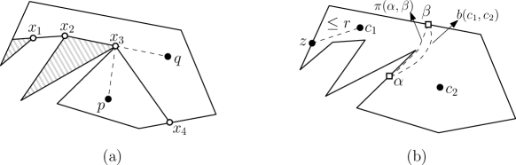
Figure 1: (a) The bisector of $p$ and $q$ contains two 2-dimensional regions (two dashed triangles). We have two line segments $x_{1}x_{2}$ and $x_{3}x_{4}$ after removing two 2-dimensional regions. Here, $b(p,q)=x_{3}x_{4}$. (b) For any point $z$ in $C[\alpha,\beta]$, we have $d(z,c_{1})\leq r$ for any radius $r$ for the geodesic disks containing $P$ centered at $c_{1}$ and $c_{2}$, where $\alpha$ and $\beta$ are the endpoints of $b(c_{1},c_{2})$.

3 The partition by a $2$-center

Although there may exist more than one geodesic $2$-center of $P$, the radius of any geodesic $2$-center is the same. Let $(c_{1}^{*},c_{2}^{*})$ be a geodesic $2$-center and $r^{*}=r_{P}(c_{1}^{*},c_{2}^{*})$. For any two points $\alpha$ and $\beta$ on $\partial P$, let $r_{\mathrm{max}}{(\alpha,\beta)}=\max\{r({\alpha},{\beta}),r({\beta},{\alpha})\}$. We say that two geodesic disks cover $P$ if the union of the two geodesic disks coincides with $P$.

Lemma 1

[19, Lemma 1] Let $a,b$ and $c$ be points in $P$. As $x$ varies along $\pi(b,c)$, $d(a,x)$ is a convex function of $d(b,x)$, and $d(a,x)\leq\max\{d(a,b),d(a,c)\}$.

Lemma 2

If $P$ is covered by two geodesic disks centered at points in $P$ with radius $r$, then there are two points $x,y\in\partial P$ with $r_{\mathrm{max}}{(x,y)}\leq r$.

Proof.  Let $c_{1}$ and $c_{2}$ be the centers of the two geodesic disks with radius $r$ covering $P$. Let $\alpha$ and $\beta$ be the two endpoints of the bisecting curve $b(c_{1},c_{2})$. We will argue that $r_{\mathrm{max}}{(\alpha,\beta)}\leq r$.

Without loss of generality, assume that $c_{1}$ lies in the subpolygon of $P$ bounded by $b(c_{1},c_{2})$ and $C[\alpha,\beta]$. Let $z$ be any point on $C[\alpha,\beta]$. See Figure 1(b). Since $P$ coincides with $D_{r}(c_{1})\cup D_{r}(c_{2})$, we have $\min\{d(z,c_{1}),d(z,c_{2})\}\leq r$. Also, since $z$ and $c_{1}$ lie in the same side of $b(c_{1},c_{2})$, we have $d(z,c_{1})\leq d(z,c_{2})$. Therefore, $d(z,c_{1})=\min\{d(z,c_{1}),d(z,c_{2})\}\leq r$.

Moreover, for any point $p\in\pi(\alpha,\beta)$, it holds that $d(c_{1},p)\leq\max\{d(c_{1},\alpha),d(c_{1},\beta)\}$ by Lemma 1. Then, since $\alpha$ and $\beta$ are the endpoints of $b(c_{1},c_{2})$, we find $\max\{d(c_{1},\alpha),d(c_{1},\beta)\}\leq r$, from which $d(c_{1},p)\leq r$. Therefore, the boundary of $P[\alpha,\beta]$ is contained in $D_{r}(c_{1})$ and so is $P[\alpha,\beta]$ by the geodesic convexity of $P[\alpha,\beta]$.

Similarly, we can show that $P[\beta,\alpha]$ is contained in $D_{r}(c_{2})$. Consequently, $r_{\mathrm{max}}{(\alpha,\beta)}\leq r$.    

For any $2$-set $(c_{1},c_{2})$ in $P$ and any radius $r$, we call a pair $(\alpha,\beta)$ of points on $\partial P$ a point-partition of $P$ with respect to $(c_{1},c_{2},r)$ if $d(c_{1},x)\leq r$ and $d(c_{2},y)\leq r$ for all points $x\in P[\alpha,\beta]$ and $y\in P[\beta,\alpha]$. Note that a point-partition with respect to $(c_{1},c_{2},r)$ does not exist if $r<r_{P}(c_{1},c_{2})$. A pair $(e,e^{\prime})$ of edges is called an edge-partition with respect to $(c_{1},c_{2},r)$ if there is a point-partition $(\alpha,\beta)$ with respect to $(c_{1},c_{2},r)$ for $\alpha\in e$ and $\beta\in e^{\prime}$. A point-partition and an edge-partition with respect to $(c_{1}^{*},c_{2}^{*},r^{*})$ are said to be optimal. By Lemma 2, there always exist an optimal point-partition and an optimal edge-partition in a simple polygon. Note that a point-partition and an edge-partition with respect to $(c_{1},c_{2},r)$ are not necessarily unique if $\min\{d(c_{1},\alpha),d(c_{1},\beta)\}<r$, where $\alpha$ and $\beta$ are the two endpoints of $b(c_{1},c_{2})$. If an optimal point-partition $(\alpha,\beta)$ of $P$ is given, we can compute a $2$-center in linear time using the algorithm in [1, 2].

Our general strategy is to first compute a set of pairs of edges, which we call candidate edge pairs, containing at least one optimal edge-partition. For each candidate edge pair $(e_{i},e_{j})$, we compute a $2$-center $(c_{1},c_{2})$ restricted to $(e_{i},e_{j})$. That is, a $2$-set $(c_{1},c_{2})$ such that $c_{1}$ and $c_{2}$ are the $1$-centers of $P[\alpha,\beta]$ and $P[\beta,\alpha]$, respectively, where $(\alpha,\beta)$ is the pair realizing $\inf_{(x,y)\in e_{i}\times e_{j}}r_{\mathrm{max}}{(x,y)}$.

3.1 Computing a set of candidate edge pairs

In this section, we define candidate edge pairs and describe how to find the set of all candidate edge pairs in $O(n^{2}\log n)$ time. Let $f(\cdot)$ be the function which maps each vertex $v$ of $P$ to the set of vertices $v^{\prime}$ of $P$ that minimize $r_{\mathrm{max}}{(v,v^{\prime})}$. It is possible that there are more than one vertex $v^{\prime}$ that minimizes $r_{\mathrm{max}}{(v,v^{\prime})}$. Moreover, such vertices appear on the boundary of $P$ consecutively. This is because the function $r({v},{x})$ is non-decreasing and $r({x},{v})$ is non-increasing as $x$ moves clockwise from $v$ along $\partial P$.

We use $f_{cw}(v)$ to denote the set of all vertices on $\partial P$ that come after $v$ and before any vertex in $f(v)$ in clockwise order. Similarly, we use $f_{ccw}(v)$ to denote the set of all vertices on $\partial P$ that come after $v$ and before any vertex in $f(v)$ in counterclockwise order. Refer to Figure 2. The three sets $f_{ccw}(v)$, $f(v)$ and $f_{cw}(v)$ are pairwise disjoint by the fact that $v\notin f(v)$ and by the monotonicity of $r({v},{x})$ and $r({x},{v})$.

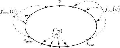
Figure 2: For a vertex $v$, we define $f_{ccw}(v)$, $f_{cw}(v)$ and $f(v)$.

Given two points $\alpha,\beta\in\partial P$, recall that we set $r({\alpha},{\beta})=r(P[\alpha,\beta])$.

Lemma 3

Given a vertex $v$ of $P$, it holds that $r({v},{w})<r({w},{v})$ for any vertex $w\in f_{cw}(v)$ and $r({v},{w})>r({w},{v})$ for any vertex $w\in f_{ccw}(v)$.

Proof.  Let us focus on the first inequality. Assume to the contrary that $r({v},{w})\geq r({w},{v})$ for some vertex $w\in f_{cw}(v)$. Let $v^{\prime}$ be a vertex in $f(v)$. Since $r({v},{v^{\prime}})\geq r({v},{w})$ and $r({w},{v})\geq r({v^{\prime}},{v})$, we have $r({v},{v^{\prime}})\geq r({v^{\prime}},{v})$. Thus $r_{\mathrm{max}}{(v,v^{\prime})}=r({v},{v^{\prime}})\geq r({v},{w})=r_{\mathrm{max}}{(v,w)}$, which contradicts the fact that $f(v)\cap f_{cw}(v)=\phi$.

We can prove the second inequality in a similar way.    

Lemma 4

Let $v$ be a vertex of $P$. For a vertex $w\in f_{cw}(v)$, it holds that $f(w)\cap C[v_{cw},w]\neq\phi$, where $v_{cw}$ is the last vertex of $f_{cw}(v)$ from $v$ in clockwise order.

Proof.  Let $w^{\prime}$ be the last vertex of $f(w)$ from $w$ in clockwise order. We show that $w^{\prime}\in C[v_{cw},w]$, which implies the lemma.

Assume to the contrary that $w^{\prime}\in C[w,v_{cw}]\setminus\{w,v_{cw}\}$. By Lemma 3 and the monotonicity of the functions $r({\cdot},{w^{\prime}})$ and $r({w^{\prime}},{\cdot})$, we have $r({w},{w^{\prime}})\leq r({v},{w^{\prime}})<r({w^{\prime}},{v})\leq r({w^{\prime}},{w})$. Similarly, we get $r({w},{v_{cw}})\leq r({v},{v_{cw}})<r({v_{cw}},{v})\leq r({v_{cw}},{w})$. Thus, $r_{\mathrm{max}}{(w,v_{cw})}=r({v_{cw}},{w})\leq r({w^{\prime}},{w})=r_{\mathrm{max}}{(w,w^{\prime})}$ by the monotonicity of $r({\cdot},{w})$. This contradicts the fact that $w^{\prime}$ is the last vertex of $f(w)$ from $w$ in clockwise order.    

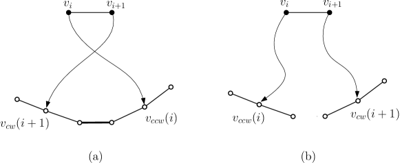
Figure 3: According to the relative positions for $v_{cw}(i+1)$ and $v_{ccw}(i)$, the candidate edges of $e_{i}$ are defined. (a) Four candidate edges of type (1) and one candidate edge of type (2). (b) Four candidate edges of type (1).

Given an edge $e_{i}=v_{i}v_{i+1}$, an edge $e_{j}=v_{j}v_{j+1}$ is called a candidate edge of $e_{i}$ if it belongs one of the following two types. For a vertex $v_{k}$, let $v_{cw}(k)$ be the last vertex of $f_{cw}(v_{k})$ from $v_{k}$ in clockwise order and $v_{ccw}(k)$ be the first vertex of $f_{ccw}(v_{k})$ from $v_{k}$ in counterclockwise order. Refer to Figure 3.

1. $v_{j}$ (or $v_{j+1}$) is $v_{ccw}(i)$ or $v_{cw}(i+1)$.

2. $e_{j}$ has both endpoints in the interior of $C[v_{ccw}(i),v_{cw}(i+1)]$ and $v_{ccw}(i)$ comes before $v_{cw}(i+1)$ from $v_{i}$ in clockwise order along $\partial P$. The edge marked with thick line segment in Figure 3(a) satisfies this condition.

A pair $(e_{i},e_{j})$ of edges is called a candidate edge pair if $e_{j}$ is a candidate edge of $e_{i}$.

Lemma 5

There is an optimal edge-partition in the set of all candidate edge pairs.

Proof.  By Lemma 2, there exists an optimal point-partition. Among all optimal point-partitions, let $(\alpha,\beta)$ be one such that $(\alpha,\beta^{\prime})$ is not an optimal point-partition for any $\beta^{\prime}\in C[\alpha,\beta]\setminus\{\beta\}$. Let $(e_{i},e_{j})$ be an optimal edge-partition with $\alpha\in e_{i}$ and $\beta\in e_{j}$. If $\beta$ is a vertex, let $e_{j}$ be an edge such that $\beta=v_{j+1}$ (so that in all cases, the counterclockwise neighbor of $\beta$ is $v_{j}$). Our goal is to show that if there is no candidate edge pair of type (1), then $(e_{i},e_{j})$ is a candidate edge pair of type (2). Thus, we need to locate $e_{j}$ with respect to $v_{ccw}(i)$ and $v_{cw}(i+1)$.

Assume that $(e_{i},e_{j})$ is not a candidate edge pair of type (1). We claim the followings.

• $v_{ccw}(i)\in C[v_{i+1},v_{j+1}]$

• $v_{cw}(i+1)\in C[v_{j},v_{i}]$

Suppose these two claims are true. Then, $v_{cw}(i+1)$ appears after $v_{ccw}(i)$ as we move clockwise from $v_{i}$ along $\partial P$ since we assume that $(e_{i},e_{j})$ is not a candidate edge pair of type (1). Moreover, $e_{j}$ has both endpoints in the interior of $C[v_{ccw}(i),v_{cw}(i+1)]$. Therefore, $(e_{i},e_{j})$ is a candidate edge pair of type (2).

It remains to prove the two claims. We start with the first one. The strategy is to show that if the first claim is not true, there is another optimal edge-partition belonging to type (1). Let $x_{i}^{\prime}\in\partial P$ be the last clockwise point from $v_{i}$ which minimizes $r_{\mathrm{max}}{(v_{i},x_{i}^{\prime})}$. By the definitions of $x_{i}^{\prime}$ and $(\alpha,\beta)$, we have

$$r_{\mathrm{max}}{(v_{i},x_{i}^{\prime})} =r(v_{i},x_{i}^{\prime}) =r(x_{i}^{\prime},v_{i}),$$

$$r_{\mathrm{max}}{(\alpha,\beta)} =r(\alpha,\beta) =r(\beta,\alpha).$$

Since $(\alpha,\beta)$ is an optimal point-partition, we have

$$r(x_{i}^{\prime},v_{i})=r_{\mathrm{max}}{(v_{i},x_{i}^{\prime})}\geq r_{\mathrm{max}}{(\alpha,\beta)}=r(\beta,\alpha).$$ (1)

If our first claim is not true, then $v_{ccw}(i)$ comes after $v_{j+1}$ in clockwise order from $v_{i}$. This implies that $x_{i}^{\prime}$ comes after $v_{j+1}$ in clockwise order from $v_{i}$. We show that $r_{\mathrm{max}}{(v_{i},x_{i}^{\prime})}=r_{\mathrm{max}}{(\alpha,\beta)}$. If not, we would have $r(x_{i}^{\prime},v_{i})>r(\beta,\alpha)$, from which, by the monotonicity of the functions $r(\beta,\cdot)$ and $r(\cdot,v_{i})$,

$$r(x_{i}^{\prime},v_{i})>r(\beta,\alpha)\geq r(\beta,v_{i})\geq r(x_{i}^{\prime},v_{i}),$$

which is a contradiction. Therefore, $r(x_{i}^{\prime},v_{i})=r(\beta,\alpha)$, which means that $(v_{i},x_{i}^{\prime})$ is an optimal point-partition since we now have $r_{\mathrm{max}}{(v_{i},x_{i}^{\prime})}=r(x_{i}^{\prime},v_{i})=r(\beta,\alpha)=r_{\mathrm{max}}{(\alpha,\beta)}$.

Let us redefine $\alpha$ as $v_{i}$ and $\beta$ as $x_{i}^{\prime}$. We also redefine $(e_{i},e_{j})$ as an optimal edge-partition such that $v_{i}=\alpha$ and $\beta\in e_{j}$ (if $\beta$ is a vertex, we choose $e_{j}$ such that $\beta=v_{j+1}$). In this way, $v_{ccw}(i)$ remains the same. Thus $v_{ccw}(i)$ is the counterclockwise neighbor of $x_{i}^{\prime}$. Therefore, $(e_{i},e_{j})$ is a candidate pair of type (1).

We now prove the second claim. The second claim can be proved in a similar way. Assume to the contrary that $v_{cw}(i+1)\in C[v_{i},v_{j}]\setminus\{v_{i},v_{j}\}$. Then $v_{cw}(i+1)$ comes before $v_{j}$ from $v_{i+1}$ in clockwise order. Let $x_{i+1}^{\prime}$ be the first clockwise point from $v_{i+1}$ that minimizes $r_{\mathrm{max}}{(v_{i+1},x_{i+1}^{\prime})}$. Thus, $x_{i+1}^{\prime}$ comes before $\beta$ from $v_{i+1}$ in clockwise order. Then the following holds:

$$r_{\mathrm{max}}{(v_{i+1},x_{i+1}^{\prime})}=r(v_{i+1},x_{i+1}^{\prime})\leq r(v_{i+1},\beta)\leq r(\alpha,\beta)=r_{\mathrm{max}}{(\alpha,\beta)}.$$

This implies that $(v_{i+1},x_{i+1}^{\prime})$ is also an optimal point-partition. We redefine $\alpha$ as $v_{i+1}$ and $\beta$ as $x_{i+1}^{\prime}$. We also redefine $e_{i}$ and $e_{j}$ accordingly. This pair $(e_{i},e_{j})$ is a candidate edge pair of type (1).

Therefore, we have an optimal edge-partition in the set of all candidate edge pairs.    

Figure 4: Two candidate edge pairs $(e_{i},e_{k})$ and $(e_{j},e_{k})$ of type (2). $e_{i}$ comes before $e_{j}$ from $e_{k}$.

Lemma 6

There are $O(n)$ candidate edge pairs.

Proof.  Since $v_{ccw}(i)$ and $v_{cw}(i)$ are uniquely defined for any vertex $v_{i}$ of $P$, the total number of candidate edge pairs of type (1) is at most $4n$.

Now we consider the candidate edge pairs which have not been counted yet. Assume that for an edge $e_{k}$ there are two distinct candidate edge pairs, say $(e_{i},e_{k})$ and $(e_{j},e_{k})$, of type (2). Without loss of generality, we assume that $e_{i}$ comes before than $e_{j}$ in clockwise order from $e_{k}$. Since they are candidate edge pairs of type (2), $e_{k}$ is contained in the intersection of $C[v_{ccw}(i),v_{cw}(i+1)]$ and $C[v_{ccw}(j),v_{cw}(j+1)]$.

We now argue that $v_{j}$ lies on $C[v_{i+1},v_{cw}(i+1)]$. Suppose that $v_{j}\in C[v_{cw}(i+1),v_{i+1}]\setminus\{v_{cw}(i+1),v_{i+1}\}$ for the sake of a contradiction. Then, since $e_{k}$ is contained in $C[v_{ccw}(i),v_{cw}(i+1)]$, the vertex $v_{j}$ lies in the interior of $C[v_{k+1},v_{i+1}]$. This contradicts the fact that $e_{i}$ comes before than $e_{j}$ in clockwise order from $e_{k}$. Therefore, $v_{j}$ lies on $C[v_{i+1},v_{cw}(i+1)]$, which means that $v_{j}\in f_{cw}(v_{i+1})$. Refer to Figure 4.

Consequently, by Lemma 4, $v_{ccw}(j)$ lies in $C[v_{cw}(i+1),v_{j}]$. Since $e_{k}$ is contained in $C[v_{ccw}(i),v_{cw}(i+1)]$, $v_{cw}(i+1)$ lies in $C[v_{k+1},v_{i}]$. This implies that $e_{k}$ is not contained in $C[v_{ccw}(j),v_{cw}(j+1)]$, which is a contradiction.

Therefore, for an edge $e$, there exists at most one edge $e^{\prime}$ such that $(e^{\prime},e)$ is a candidate edge pair of type (2). Thus the number of candidate edge pairs of type (2) is $O(n)$.    

Now we present a procedure for finding the set of all candidate edge pairs. For each index $i$, we compute $v_{cw}(i)$ and $v_{ccw}(i)$ in $O(n\log n)$ time. To find $v_{cw}(i)$, we apply binary search on the vertices of $P$ using Lemma 3 and a linear-time algorithm [1, 2] that computes the center of a simple polygon. We can find $v_{ccw}(i)$ in a similar way. This takes $O(n^{2}\log n)$ time in total.

Then, we compute the set of all candidate edge pairs based on the information we just computed. For each edge $e_{i}$, we consider the edges lying between $v_{ccw}(i)$ and $v_{cw}(i+1)$ if $v_{ccw}(i)$ comes before $v_{cw}(i+1)$ from $v_{i}$ in clockwise order. Otherwise, we consider the four edges incident to $v_{ccw}(i)$ and $v_{cw}(i+1)$. In total, this takes time linear to the number of candidate edge pairs, which is $O(n)$ by Lemma 6.

Lemma 7

The set of all candidate edge pairs can be computed in $O(n^{2}\log n)$ time.

4 A decision algorithm for a candidate edge pair

We say that a point-partition $(\alpha,\beta)$ is restricted to $(e_{i},e_{j})$ if $\alpha\in e_{i}$ and $\beta\in e_{j}$. We say that a triplet $(c_{1},c_{2},r)$ consisting of a $2$-set $(c_{1},c_{2})$ and a radius $r$ is restricted to $(e_{i},e_{j})$ if some point-partitions with respect to $(c_{1},c_{2},r)$ are restricted to $(e_{i},e_{j})$. We consider $r_{\mathrm{max}}{(\alpha,\beta)}$ as a function whose variables are $\alpha\in e_{i}$ and $\beta\in e_{j}$. Since the function is continuous and the domain is bounded, there exist two points, $\alpha^{*}\in e_{i}$ and $\beta^{*}\in e_{j}$, that minimize the function. We call $(c_{1}^{*},c_{2}^{*})$ a $2$-center restricted to $(e_{i},e_{j})$ if $c_{1}^{*}$ and $c_{2}^{*}$ are the $1$-centers of $P[\alpha^{*},\beta^{*}]$ and $P[\beta^{*},\alpha^{*}]$, respectively. By Lemma 5, there is a $2$-center restricted to a candidate edge pair which is a $2$-center (without any restriction).

In this section, we present a decision algorithm for a candidate edge pair $(e_{i},e_{j})$. Let $r_{ij}^{*}$ be the radius of a $2$-center restricted to $(e_{i},e_{j})$. Let $r$ be an input of the algorithm. The decision algorithm in this section returns “yes” if $r\geq r_{ij}^{*}$. Additionally, it returns a $2$-center restricted to $(e_{i},e_{j})$ with radius $r$. It returns “no”, otherwise.

Throughout this section, we assume that $r({v_{i+1}},{v_{j}})\leq r<r({v_{i}},{v_{j+1}})$ and $r({v_{j+1}},{v_{i}})\leq r<r({v_{j}},{v_{i+1}})$ because the other cases can be handled easily: if $r({v_{j+1}},{v_{i}})>r$ or $r({v_{i+1}},{v_{j}})>r$, we return “no”. For the remaining cases, we return “yes”.

The decision algorithm first assumes that $r\geq r_{ij}^{*}$ and constructs a $2$-center restricted to $(e_{i},e_{j})$ with radius $r$. The $2$-center produced by the algorithm is valid if and only if $r\geq r_{ij}^{*}$. Therefore, the algorithm can then decide whether $r\geq r_{ij}^{*}$ by checking whether the $2$-center is valid. Thus, from now on, we assume that $r\geq r_{ij}^{*}$. Let $(c_{1},c_{2},r)$ be a triplet consisting of a $2$-set $(c_{1},c_{2})$ and radius $r$ which is restricted to $(e_{i},e_{j})$, and $(\alpha,\beta)$ be a point-partition with respect to $(c_{1},c_{2},r)$ which is restricted to $(e_{i},e_{j})$. Without loss of generality, we assume that $D_{r}(c_{1})$ contains $P[\alpha,\beta]$ and $D_{r}(c_{2})$ contains $P[\beta,\alpha]$.

4.1 Computing the intersection of geodesic disks

The first step of the decision algorithm is to compute the intersection $I_{1}$ of the geodesic disks of radius $r$ centered at $v\in C[v_{i+1},v_{j}]$ and the intersection $I_{2}$ of the geodesic disks of radius $r$ centered at $v\in C[v_{j+1},v_{i}]$, that is, $I_{1}=\cap_{k=i+1}^{j}{D_{r}(v_{k})}$ and $I_{2}=\cap_{k=j+1}^{i}{D_{r}(v_{k})}$. Clearly, $c_{1}\in I_{1}$ and $c_{2}\in I_{2}$.

We compute $I_{1}$ and $I_{2}$ by constructing the farthest-point geodesic Voronoi diagrams, denoted by $\mathsf{FV}_{1}$ and $\mathsf{FV}_{2}$, of the vertices in $C[v_{i+1},v_{j}]$ and the vertices in $C[v_{j+1},v_{i}]$, respectively. For the case that the sites are on the vertices of $P$, the diagram can be computed in $O(n\log\log n)$ time [18].

A cell in $\mathsf{FV}_{1}$ associated with a site $t$ consists of the points $p\in P$ such that $t$ is the site farthest from $p$ among all sites. A refined cell in $\mathsf{FV}_{1}$ associated with site $t$ is obtained by further subdividing the cell associated with site $t$ such that all points in the same refined cell have the same combinatorial structure of the shortest paths from their common farthest site. While constructing $\mathsf{FV}_{1}$ and $\mathsf{FV}_{2}$, the algorithm [18] computes all refined cells. For each refined cell, we can store the information of the common farthest site $t$ of the refined cell and the anchor of $\pi(t,p)$ closest to $p$ for a point $p$ in the refined cell.

Then we compute circular arcs of $\partial I_{1}$ and $\partial I_{2}$ contained in a refined cell in time linear to the number of circular arcs in that refined cell plus the complexity of the refined cell. By traversing all refined cells, we can compute all circular arcs in $O(n)$ time by the following lemma.

Lemma 8

The total number of circular arcs in $\partial I_{1}$ and $\partial I_{2}$ is $O(n)$.

Proof.  We prove the lemma only for $\partial I_{1}$. The case for $\partial I_{2}$ can be proven analogously. The size of the (refined) farthest-point geodesic Voronoi diagram of $n$ sites in a simple polygon with $n$ vertices is $O(n)$ [3]. In other words, there are $O(n)$ refined cells and edges of the Voronoi diagram.

Let $s$ be a circular arc of $\partial I_{1}$. The center $c_{s}$ of the geodesic disk containing $s$ on its boundary lies in $C[v_{i+1},v_{j}]$. Note that $c_{s}$ is unique by the general position assumption. Every geodesic disk whose center is a vertex in $C[v_{i+1},v_{j}]\setminus\{c_{s}\}$ with radius $r$ contains $s$ in its interior. This means that, for any point $x\in s$, the farthest vertex from $x$ in $C[v_{i+1},v_{j}]$ is $c_{s}$. Moreover, the combinatorial structures of the geodesic paths from the center $c_{s}$ to points on the circular arc $s$ are the same. Thus each circular arc $s$ is contained in a refined cell of $\mathsf{FV}_{1}$ whose site is $c_{s}$. Moreover, each endpoint of the circular arc lies in the boundary of the refined cell containing it (including the boundary of $P$.) Each edge of the diagram is intersected by at most one circular arc of $\partial I_{1}$. Therefore, the number of circular arcs in $\partial I_{1}$ is $O(n)$ by the fact that the size of the refined farthest-point geodesic Voronoi diagram is $O(n)$.    

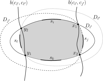
Figure 5: The center of $D_{i^{\prime}}$ must lie to either the right of $b(c_{i^{\prime}},c_{j^{\prime}})$ or the left of $b(c_{i^{\prime}},c_{\ell^{\prime}})$.

Lemma 9

Let $\mathcal{D}=\{D_{1},\ldots,D_{k}\}$ be a set of geodesic disks with the same radius and let $I$ be the intersection of all geodesic disks in $\mathcal{D}$. Let $S=\langle s_{1},\ldots,s_{k^{\prime}}\rangle$ be the cyclic sequence of the circular arcs of $\partial I$ along its boundary in clockwise order. For any integer $i\in[1,k]$, the circular arcs in $\partial I\cap\partial D_{i}$ are consecutive in $S$.

Proof.  Assume to the contrary that there are four circular arcs $s_{i},s_{j},s_{k},s_{\ell}$ in $S$ with $i<j<k<\ell$ such that $s_{i},s_{k}\subset\partial D_{i^{\prime}}$, $s_{j}\subset\partial D_{j^{\prime}}$ and $s_{\ell}\subset\partial D_{\ell^{\prime}}$ for three distinct geodesic disks $D_{i^{\prime}},D_{j^{\prime}},D_{\ell^{\prime}}\in\mathcal{D}$. See Figure 5. Let $c_{i^{\prime}},c_{j^{\prime}},c_{\ell^{\prime}}$ be the centers of the disks $D_{i^{\prime}},D_{j^{\prime}},D_{\ell^{\prime}}$, respectively. Then the bisecting curve of $c_{i^{\prime}}$ and $c_{j^{\prime}}$ intersects $\partial(D_{i^{\prime}}\cup D_{j^{\prime}})$ exactly twice. Let $x_{1}$ and $x_{2}$ be these two intersection points such that $s_{j}$ is contained in the region bounded by $b(c_{i^{\prime}},c_{j^{\prime}})$ and the part of $\partial D_{i^{\prime}}$ from $x_{1}$ to $x_{2}$ in clockwise order. Similarly, the bisecting curve of $c_{i^{\prime}}$ and $c_{\ell^{\prime}}$ intersects $\partial(D_{i^{\prime}}\cup D_{\ell^{\prime}})$ exactly twice. Let $y_{1}$ and $y_{2}$ be these intersection points such that $s_{\ell}$ is contained in the region bounded by $b(c_{i^{\prime}},c_{\ell^{\prime}})$ and the part of $\partial D_{i^{\prime}}$ from $y_{1}$ to $y_{2}$ in clockwise order. When we traverse $\partial I$ clockwise starting from $s_{i}$, we encounter $x_{1}$, $\mathrm{int}(s_{j})$, $x_{2}$, $\mathrm{int}(s_{k})$, $y_{1}$ $\mathrm{int}(s_{\ell})$, and $y_{2}$ in order, where $\mathrm{int}(s)$ is the circular arc $s$ excluding its endpoints for a circular arc $s$.

The center $c_{i^{\prime}}$ lies in the subset $P_{1}\subset D_{i^{\prime}}$ bounded by $b(c_{i^{\prime}},c_{j^{\prime}})$ and the part of $\partial I$ from $x_{1}$ to $x_{2}$ in clockwise order. On the other hand, $c_{i^{\prime}}$ lies in the subset $P_{2}\subset D_{i^{\prime}}$ bounded by $b(c_{i^{\prime}},c_{\ell^{\prime}})$ and the part of $\partial I$ from $y_{1}$ to $y_{2}$ in clockwise order. Thus, $c_{i^{\prime}}\in P_{1}\cap P_{2}$. Therefore, $P_{1}$ and $P_{2}$ must intersect. Since $c_{i^{\prime}}$ lies in the interior of $D_{i^{\prime}}$, $b(c_{i^{\prime}},c_{\ell^{\prime}})$ and $b(c_{i^{\prime}},c_{j^{\prime}})$ must intersect in the interior of $D_{i^{\prime}}$. In order to satisfy the order of appearances of $x_{1}$, $x_{2}$, $y_{1}$ and $y_{2}$ along $\partial I$, $b(c_{i^{\prime}},c_{\ell^{\prime}})$ and $b(c_{i^{\prime}},c_{j^{\prime}})$ must intersect an even number of times in the interior of $D_{i^{\prime}}$. This is impossible since $b(x,y)$ and $b(x,z)$ cross each other at most once for any three points $x,y,z$ in $P$. Thus $P_{1}\cap P_{2}=\phi$, which is a contradiction.    

Note that $\partial I_{1}$ and $\partial I_{2}$ consist of $O(n)$ circular arcs and (possibly incomplete) edges of $\partial P$ in total. Let $S_{1}$ and $S_{2}$ be the unions of the circular arcs of $\partial I_{1}$ and $\partial I_{2}$, respectively. By the following lemma, it is sufficient to choose two points, one from $S_{1}$ and one from $S_{2}$, in order to find a $2$-center restricted to $(e_{i},e_{j})$ with radius $r$.

Lemma 10

If $r_{ij}^{*}\leq r\leq\min\{r({v_{i}},{v_{j+1}}),r({v_{j}},{v_{i+1}})\}$, there is a triplet $(c_{1},c_{2},r)$ restricted to $(e_{i},e_{j})$ such that $c_{1}\in S_{1}$ and $c_{2}\in S_{2}$.

Proof.  Since $r_{ij}^{*}\leq r$, there is a triplet $(c_{1}^{\prime},c_{2}^{\prime},r)$ made of a $2$-set $(c_{1}^{\prime},c_{2}^{\prime})$ and a radius $r$ restricted to $(e_{i},e_{j})$. Let $(\alpha,\beta)$ be a point-partition with respect to $(c_{1}^{\prime},c_{2}^{\prime},r)$ with $\alpha\in e_{i}$ and $\beta\in e_{j}$. Without loss of generality, we assume that $c_{1}^{\prime}\in P[\alpha,\beta]$ and $c_{2}^{\prime}\in P[\beta,\alpha]$.

Consider $c_{1}^{\prime}$ first. Let $x\in e_{i}$ be the point closest to $v_{i}$ among the points satisfying $d(x,c_{1}^{\prime})\leq r$. Similarly, let $y\in e_{j}$ be the point closest to $v_{j+1}$ among the points satisfying $d(y,c_{1}^{\prime})\leq r$. Then we have $r({x},{y})\leq r$. As we move $x$ from its current position to $v_{i}$ along $e_{i}$, $r({x},{y})$ increases. We move $x$ until $r({x},{y})=r$ or $x$ reaches $v_{i}$. If $x$ reaches $v_{i}$, we move $y$ from the current position to $v_{j+1}$ until $r({x},{y})=r$. This is always possible to find such $x$ and $y$ since, by the assumption, we have $r({v_{i}},{v_{j+1}})\geq r$.

Now we consider the subpolygon $P[x,y]$. Let $c_{1}$ be the center of $P[x,y]$. If there is a vertex $v\in C[x,y]$ with $d(v,c_{1})=r$, then $c_{1}$ lies in $S_{1}$ and $D_{r}(c_{1})$ contains $D_{r}(c_{1}^{\prime})$, thus we are done. Otherwise, $c_{1}$ is the midpoint of $\pi(x,y)$. But then, since $D_{r}(c_{2}^{\prime})$ contains $x$ and $y$, this means that $c_{2}^{\prime}=c_{1}$, which is a contradiction. Thus, the pair $(c_{1},c_{2}^{\prime})$ is a $2$-center restricted to $(e_{i},e_{j})$ and $c_{1}\in S_{1}$.

Similarly, we can find $c_{2}$ lying in $S_{2}$ with $D_{r}(c_{2}^{\prime})\subset D_{r}(c_{2})$.    

4.2 Subdividing the edges and the boundaries of the intersections

The shortest path map rooted at $x$ is the subdivision of $P$ consisting of triangular cells such that every point $p$ in the same cell has the same combinatorial structure of $\pi(p,x)$. The map can be obtained by extending the edges of the shortest path tree rooted at $x$ towards their descendants [11]. Let $\mathsf{SPM}_{k}$ denote the shortest path map rooted at $v_{k}$. We compute the shortest path maps $\mathsf{SPM}_{i}$ and $\mathsf{SPM}_{i+1}$.

By overlaying the two shortest path maps with $\partial I_{1}$, we obtain the set of $O(n)$ finer arcs of $\partial I_{1}$ as follows. We find any cell of $\mathsf{SPM}_{i}$ intersecting $\partial I_{1}$, and traverse to the neighboring cells along $\partial I_{1}$. Whenever we cross an edge of the cell along an arc of $\partial I_{1}$, we compute the intersection between the edge of the cell and the arc of $\partial I_{1}$. We can check in constant time whether a given arc of $\partial I_{1}$ crosses an edge of a given cell in $\mathsf{SPM}_{i}$ since every cell is a triangle. While traversing $\partial I_{1}$, we cross each edge of $\mathsf{SPM}_{i}$ at most twice by the geodesic convexity of $I_{1}$. Thus, in total, it is sufficient to traverse $\partial I_{1}$ once and cross each edge in $\mathsf{SPM}_{i}$ at most twice. Similarly, we compute the intersections between $\partial I_{1}$ and $\mathsf{SPM}_{i+1}$. From now on, we treat $\partial I_{1}$ as the sequence of $O(n)$ finer arcs.

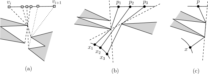
Figure 6: (a) By extending the edges of the shortest path trees rooted at $v_{i}$ and rooted at $v_{i+1}$, we obtain subedges of $e_{i}=v_{i}v_{i+1}$. The endpoints of the subedges are marked with squares. (b) If the geodesic path $\pi(x,p)$ is elementary, there are at most three different combinatorial structures of $\pi(x,p)$ depending on $x$ and $p$. (c) For any point $x$ in the finer circular arc and any point $p$ in the subedge, the combinatorial structures of $\pi(x,p)$ are the same for all $x$ and $p$.

We also subdivide the polygon edge $e_{i}$ into $O(n)$ subedges by overlaying the extensions of the edges in the shortest path trees rooted at $v_{i}$ and $v_{i+1}$ towards their parents with $e_{i}$. See Figure 6(a). Let $\mathcal{L}_{i}$ be the set of intersections of the extensions of the edges in the shortest path trees of $v_{i}$ and $v_{i+1}$ with $e_{i}$. While computing $\mathcal{L}_{i}$, we sort them along $e_{i}$ from $v_{i+1}$. This takes $O(n\log n)$ time. We compute $\mathcal{L}_{j}$ similarly, which is the set of the intersections of the extensions of the edges in $\mathsf{SPM}_{j}$ and $\mathsf{SPM}_{j+1}$ with $e_{j}$, and sort them along $e_{j}$ from $v_{j}$.

We say that a geodesic path between two points is elementary if the number of line segments in the geodesic path is at most two. If $\pi(x,p)$ is elementary for all points $x$ on the same finer arc of $\partial I_{1}$ and all points $p$ on the same subedge, there are at most three possible distinct combinatorial structures as shown in Figure 6(b). However, the combinatorial structures of $\pi(x,p)$ are the same for any point $x$ on the same finer circular arc and any point $p$ on the same subedge if $\pi(x,p)$ is not elementary for all $x$ and $p$. Refer to Figure 6(c).

4.3 Four coverage functions and their extrema

In this section, we will subdivide $\partial I_{1}$ and $\partial I_{2}$ into $O(1)$ subchains (refer to Subsection 4.3.2). Then for every pair of subchains, one from $\partial I_{1}$ and one from $\partial I_{2}$, we will explain how to decide whether there is a $2$-center $(c_{1},c_{2})$ restricted to a candidate edge pair lying on the two subchains in Section 4.4. To this end, in the following subsection, we define four functions $\phi_{t}(x)$ and $\psi_{t}(x)$ for $t=1,2$.

4.3.1 Four coverage functions

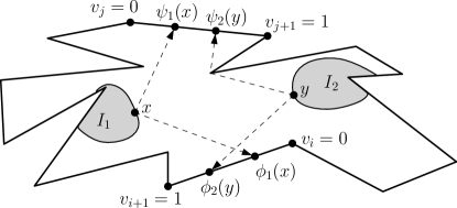
Figure 7: For a point $x\in\partial I_{t}$, it holds that $d(\phi_{t}(x),x)=r$ and $d(\psi_{t}(x),x)=r$ if $d(v_{i},x)\geq r$ and $d(v_{j+1},x)\geq r$ for $t=1,2$.

We represent each point $p\in e_{i}$ as a real number in $[0,1]$: A point $x\in e_{i}$ (and $y\in e_{j}$) is represented as $\|v_{i}-p\|/\|v_{i}-v_{i+1}\|$ in $[0,1]$, where $\|x-y\|$ is the Euclidean distance between two points $x$ and $y$. Similarly, we represent each point $q\in e_{j}$ as $\|v_{j}-q\|/\|v_{j}-v_{j+1}\|$. We use a real number in $[0,1]$ and its corresponding point interchangeably. Recall that $S_{1}$ and $S_{2}$ are the unions of the circular arcs of $\partial I_{1}$ and $\partial I_{2}$, respectively.

Let us define the four functions $\phi_{t}(x)$ and $\psi_{t}(x)$ for $t=1,2$ as follows. Refer to Figure 7.

• The function $\phi_{1}:S_{1}\rightarrow[0,1]$ maps $x\in S_{1}$ to the infimum of the numbers which represent the points in $D_{r}(x)\cap e_{i}$.

• The function $\phi_{2}:S_{2}\rightarrow[0,1]$ maps $x\in S_{2}$ to the supremum of the numbers which represent the points in $D_{r}(x)\cap e_{i}$.

• The function $\psi_{1}:S_{1}\rightarrow[0,1]$ maps $x\in S_{1}$ to the supremum of the numbers which represent the points in $D_{r}(x)\cap e_{j}$.

• The function $\psi_{2}:S_{2}\rightarrow[0,1]$ maps $x\in S_{2}$ to the infimum of the numbers which represent the points in $D_{r}(x)\cap e_{j}$.

In the following, let $t$ be $1$ or $2$. Our goal is to split $S_{t}$ into subchains such that $\phi_{t}$ and $\psi_{t}$ are monotone when their domain is restricted to each subchain. However, $S_{t}$ is not necessarily a connected subset of $\partial I_{t}$. Thus, to simplify the description of the split, we define four continuous functions $\phi^{\prime}_{t},\psi^{\prime}_{t}$ : $\partial I_{t}\rightarrow[0,1]$ by interpolating $\phi_{t}$ and $\psi_{t}$ on $\partial I_{t}$:

$$\phi^{\prime}_{t}(x)=\begin{cases}\phi_{t}(x)&\quad\text{if }x\in S_{t}\\ \frac{d_{c}(x_{1},x)}{d_{c}(x_{2},x_{1})}\phi_{t}(x_{1})+\frac{d_{c}(x_{2},x)}{d_{c}(x_{2},x_{1})}\phi_{t}(x_{2})&\quad\text{otherwise,}\\ \end{cases}$$

where $x_{1}$ and $x_{2}$ are the first and the last points of $S_{t}$ along $\partial I_{t}$ from $x$ in clockwise order, respectively, and $d_{c}(x^{\prime},y^{\prime})$ denotes the length of a chain $C[x^{\prime},y^{\prime}]$. The function $\psi_{t}^{\prime}$ is defined similarly.

Lemma 11

The functions $\phi^{\prime}_{t}$ and $\psi^{\prime}_{t}$ for $t=1,2$ are well-defined.

Proof.  Here we prove the lemma only for $\phi^{\prime}_{1}$. For the other functions, the lemma can be proved analogously.

If $\phi_{1}(x)$ is well-defined, so is $\phi_{1}^{\prime}(x)$. Thus, we show that $\phi_{1}(x)$ is well-defined. The set $S_{1}$ is the domain of $\phi_{1}$ and $e_{i}$ is the range of $\phi_{1}$. Since $D_{r}(v_{i+1})$ contains all points in $S_{1}$, $D_{r}(x)$ contains $v_{i+1}$ for all $x\in S_{1}$. For each point $x\in S_{1}$, there are two cases: $D_{r}(x)$ intersects $e_{i}$ or contains $v_{i}$. For the first case, $\phi_{1}(x)$ represents the point closest to $v_{i}$ among the points $p\in e_{i}$ with $d(x,p)=r$. For the second case, $\phi_{1}(x)$ is $1$, which represents $v_{i+1}$. Thus, $\phi_{1}(x)$ is uniquely defined for a point $x\in S_{1}$, which means that it is well-defined.    

We choose any two points $w_{1}\in\partial I_{1}$ and $w_{2}\in\partial I_{2}$ which are endpoints of some circular arcs of $\partial I_{1}$ and $\partial I_{2}$, respectively, such that $d(w_{t},v_{i})<r$ and $d(w_{t},v_{j+1})<r$. Such points always exist by the assumption that $r(v_{i},v_{j+1})<r$. We use them as reference points for $\partial I_{1}$ and $\partial I_{2}$. We write $p\prec q$ for any two points $p\in\partial I_{t}$ and $q\in\partial I_{t}$, if $p$ comes before than $q$ when we traverse $\partial I_{t}$ in clockwise order from the reference point $w_{t}$ for $t=1,2$. We consider $\partial I_{1}$ and $\partial I_{2}$ as chains of circular and linear arcs starting from $w_{1}$ and $w_{2}$, respectively.

In the following, we consider the local extrema of the four functions. For the function $\phi_{t}^{\prime}$, let $N_{\max}$ be the set of points $x^{\prime}\in I_{t}\setminus\{w_{t}\}$ such that $\phi_{t}^{\prime}(x)$ has a local maximum at $x=x^{\prime}$. Similarly, let $N_{\min}$ be the set of points $x^{\prime}\in I_{t}\setminus\{w_{t}\}$ such that $\phi_{t}^{\prime}(x)$ has a local minimum at $x=x^{\prime}$. Then the following lemma holds.

Lemma 12

Both $N_{\max}$ and $N_{\min}$ are connected.

Proof.  We first consider the case that $\phi_{1}^{\prime}(x)\neq 1$ for some $x\in N_{\max}$. The boundary of $D_{r}(\phi_{1}^{\prime}(x))$ intersects $\partial I_{1}$ at $x$. Moreover, there exists a connected region $N(x)\subset\partial I_{1}$ containing $x$ such that $D_{r}(\phi_{1}^{\prime}(x))\cap N(x)=\{x\}$. Together with Lemma 9, this implies that $D_{r}(\phi_{1}^{\prime}(x))$ does not contain any point other than $x$. Thus, $x$ is the only point contained in $N_{\max}$.

For the remaining case that $\phi_{1}^{\prime}(x)=1$ for any point $x$ in $N_{\max}$, Lemma 9 implies that $D_{r}(\phi_{1}^{\prime}(x))\cap\partial I_{1}$ is connected. By definition, $N_{\max}=D_{r}(\phi_{1}^{\prime}(x))\cap\partial I_{1}$, which is connected.

Similarly, we can prove that $N_{\min}$ is connected.    

Let $x_{\max}$ and $x_{\min}$ be any two points in $N_{\max}$ and $N_{\min}$, respectively. To make the description easier, we assume that $x_{\max}\prec x_{\min}$.

The following corollary states Lemma 11 from a different point of view.

Corollary 13

The function $\phi_{1}$ is monotonically increasing in the domain $\{x\in S_{1}:x\prec x_{\max}\}$ and in the domain $\{x\in S_{1}:x_{\min}\prec x\}$ and monotonically decreasing in the domain $\{x\in S_{1}:x_{\max}\prec x\prec x_{\min}\}$.

4.3.2 Subdividing the chains with respect to local extrema

We first compute one local maximum and one local minimum for each function. Here we describe a way to find a local maximum of $\phi_{1}^{\prime}$ lying on $S_{1}$. For a point $x$ lying on $S_{1}$, it holds that $\phi_{1}^{\prime}(x)=\phi_{1}(x)$ by definition. Consider the sequence of the endpoints of the finer circular arcs starting from the reference point $w_{1}$. There are $O(n)$ endpoints. First we choose the median $w$ of the endpoints. Let $w^{\prime}$ be the endpoint adjacent to $w$ on $S_{1}$ such that $w^{\prime}\prec w$. Then we compute $\phi_{1}(w)$ and $\phi_{1}(w^{\prime})$. This takes $O(\log^{2}n)$ time by the following lemma.

Lemma 14

For a given point $x\in S_{1}$, $\phi_{1}(x)$ can be computed in $O(\log^{2}n)$ time once the shortest path trees rooted at $v_{i}$ and $v_{i+1}$ are constructed.

Proof.  The function $d(z,x)$ for $z\in e_{i}$ is convex for a fixed point $x$ by Lemma 1. Moreover, $d(v_{i},x)\leq r$ and $d(v_{i+1},x)\geq r$ since $\phi_{1}$ is well-defined. As we saw before, $\mathcal{L}_{i}$ subdivides the edge $e_{i}$ into $O(n)$ subedges. For any point $p$ on the same subedge, the combinatorial structure of the geodesic path $\pi(p,x)$ is the same.

To compute $\phi_{1}(x)$, we apply binary search on $\mathcal{L}_{i}$. First, we choose the median $p_{\mathrm{med}}$ of $\mathcal{L}_{i}$. If $d(p_{\mathrm{med}},x)>r$, then $\phi_{1}(x)$ lies between $v_{i}$ and $p_{\mathrm{med}}$, and we search the points in $\mathcal{L}_{i}$ lying between them. Otherwise, $\phi_{1}(x)$ lies between $v_{\mathrm{med}}$ and $v_{i+1}$. In either way, we can ignore half of the current search space. After $O(\log n)$ iterations, we can narrow the search space into the subedge containing $\phi_{1}(x)$. Once we find the subedge which contains $\phi_{1}(x)$, we can find the point in constant time.

Since computing the geodesic distance between two points takes $O(\log n)$ time and the number of iterations is $O(\log n)$, the time complexity for computing $\phi_{1}(x)$ is $O(\log^{2}n)$ for a point in $S_{1}$.    

If $\phi_{1}(w)=1$, $w$ is a local maximum of $\phi_{1}^{\prime}$ lying on $S_{1}$. If $\phi_{1}(w_{1})<\phi_{1}(w^{\prime})<\phi_{1}(w)$, then a local maximum comes after $w^{\prime}$. Thus, we only consider the endpoints which come after $w^{\prime}$. Otherwise, a local maximum comes before $w$ by Corollary 13. After $O(\log n)$ iterations, we can find the finer circular arc $s_{\max}$ in $S_{1}$ which contains a local maximum point.

The remaining step is to find a local maximum point on the finer circular arc $s_{\max}$. Now, we search the edge $e_{i}$ to find the interval of $\mathcal{L}_{i}$ containing a local maximum of $\phi^{\prime}_{1}$. Let $p$ be the median of $\mathcal{L}_{i}$. If $D_{r}(p)$ contains or intersects $s_{\max}$, we search further the points of $\mathcal{L}_{i}$ which come after $p$. Otherwise, we search the points of $\mathcal{L}_{i}$ which come before $p$. By the construction of $\mathcal{L}_{i}$, the number of different combinatorial structures of $\pi(x,p)$ for a point $x$ in the same circular arc and a point $p$ in the same subedge is at most three (see Figure 6). Thus, in constant time, we can check whether $D_{r}(p)$ contains or intersects $s_{\max}$.

After $O(\log n)$ iterations, we find the subedge that contains a local maximum of $\phi_{1}^{\prime}$. Then we find a local maximum in the finer circular arc in constant time. Similarly, we compute a local maximum and a local minimum for the other functions.

Therefore, we have the following lemma.

Lemma 15

A local maximum and a local minimum for $\phi_{t}^{\prime}$ (or $\psi_{t}^{\prime}$) can be computed in $O(\log^{3}n)$ time.

These local extrema subdivide $\partial I_{1}$ into at most five subchains $c_{1,k}$ for $k\in\{1,2,\ldots,5\}$ as follows. Let $x_{1},x_{2},x_{3}$ and $x_{4}$ be the local maxima and the local minima of $\phi_{1}^{\prime}$ and $\psi_{1}^{\prime}$ with $x_{1}\prec x_{2}\prec x_{3}\prec x_{4}$. The subchain $c_{1,k}$ is the set of points $x\in\partial I_{1}$ with $x_{k-1}\prec x\prec x_{k}$ for $k\in\{1,2,\ldots,5\}$, where we set $x_{0}=x_{5}=w_{1}$. After subdividing $\partial I_{1}$, $\phi_{1}$ and $\psi_{1}$ are monotone when the domain is restricted to $c_{1,k}\cap S_{1}$ for $k\in\{1,2,\ldots,5\}$. Similarly, the local extrema of $\phi_{2}^{\prime}$ and $\psi_{2}^{\prime}$ subdivide the chain $\partial I_{2}$ into five subchains $c_{2,\ell}$ ($\ell\in\{1,2,\ldots,5\}$ ). The functions $\phi_{2}$ and $\psi_{2}$ restricted to $c_{2,\ell}\cap S_{2}$ for $\ell\in\{1,2,\ldots,5\}$ are monotone.

4.4 Computing a $2$-center restricted to a pair of subchains

We consider a pair $(c_{1,k},c_{2,\ell})$ of subchains for $k\in\{1,2,\ldots,5\}$ and $\ell\in\{1,2,\ldots,5\}$. Let $s_{1,k}=S_{1}\cap c_{1,k}$ and $s_{2,\ell}=S_{2}\cap c_{2,\ell}$. We find a $2$-center with radius $r$ that is restricted to $(e_{i},e_{j})$, if it exists, where one center is on $s_{1,k}$ and the other is on $s_{2,\ell}$. Assume that $\phi_{1}$ and $\psi_{1}$ are decreasing when their domains are restricted to $s_{1,k}$. That is, for any two points $x$ and $x^{\prime}$ in $S_{1,k}$ with $x\prec x^{\prime}$, it holds that $\phi_{1}(x^{\prime})\leq\phi_{1}(x)$ and $\psi_{1}(x^{\prime})\leq\psi_{1}(x)$. Similarly, assume that $\phi_{2}$ and $\psi_{2}$ are decreasing when their domains are restricted to $s_{2,\ell}$. The other cases where some functions are increasing and the others are decreasing can be handled in a similar way.

We define two new functions $\mu_{1}:s_{1,k}\rightarrow s_{2,\ell}$ and $\mu_{2}:s_{1,k}\rightarrow s_{2,\ell}$. For a point $x\in s_{1,k}$, $\mu_{1}(x)$ denotes the last clockwise point in $s_{2,\ell}$ which is contained in $D_{r}(\phi_{1}(x))$. Similarly, for a point $x\in s_{1,k}$, $\mu_{2}(x)$ denotes the first clockwise point in $s_{2,\ell}$ which is contained in $D_{r}(\psi_{1}(x))$. If every point in $s_{2,\ell}$ is contained in $D_{r}(\phi_{1}(x))$, then $\mu_{1}(x)$ is the last clockwise point of $s_{2,\ell}$. Notice that $\mu_{1}(x)$ and $\mu_{2}(x)$ are increasing on $s_{1,k}$. If there is a point $x\in s_{1,k}$ such that $\mu_{2}(x)\prec\mu_{1}(x)$, the triplet $(x,\mu_{1}(x),r)$ is restricted to $(e_{i},e_{j})$. Moreover, for a 2-center $(c_{1},c_{2})$ restricted to $(e_{i},e_{j})$ with $c_{1}\in s_{1,k}$ and $c_{2}\in s_{2,\ell}$, it holds that $\mu_{2}(c_{1})\prec c_{2}\prec\mu_{1}(c_{1})$. Thus, we are going to find a point $x\in s_{1,k}$ such that $\mu_{2}(x)\prec\mu_{1}(x)$.

To check whether there exists such a point, we traverse $c_{1,k}$ twice. In the first traversal, we pick $O(n)$ points, which are called event points. While picking such points, we compute $\mu_{1}(x)$ and $\mu_{2}(x)$ for every event point $x$ in linear time. Then we traverse the two subchains again and find a $2$-center using the information we just computed.

Definition of the event points on $c_{1,k}$.

We explain how we define the event points on $c_{1,k}$. The set of event points of $c_{1,k}$ is the subset of $c_{1,k}$ consisting of points belonging to one of the three types defined below.

• (T1) The endpoints of all finer arcs. Recall that the subchain $c_{1,k}\subseteq\partial I_{1}$ consists of circular arcs and line segments, and it is subdivided into finer arcs by the four shortest path maps in Section 4.2.

• (T2) The points $x\in s_{1,k}$ such that $d(x,p)=r$ for some $p\in\mathcal{L}_{i}$

• (T3) The points $x\in s_{1,k}$ such that $d(x,p)=r$ for some $p\in\mathcal{L}_{j}$

Let $\mathcal{E}_{1}$, $\mathcal{E}_{2}$ and $\mathcal{E}_{3}$ be the sets of event points of types T1, T2 and T3, respectively. Let $\mathcal{E}=\mathcal{E}_{1}\cup\mathcal{E}_{2}\cup\mathcal{E}_{3}$. We say $\eta\in\mathcal{E}$ is caused by $p$ if $d(\eta,p)=r$ for $p\in\mathcal{L}_{i}\cup\mathcal{L}_{j}$.

Recall that $\mathcal{L}_{i}$ is the set of intersection points of the extensions of the edges in the two shortest path trees rooted at $v_{i}$ and rooted at $v_{i+1}$ with $e_{i}$, which has already been constructed in a previous step. Let $\mathcal{L}_{i}=\{v_{i}=p_{1},\ldots,p_{m}=v_{i+1}\}$, where the points are labeled in clockwise order from $v_{i}$.

Computation of the event points on $c_{1,k}$.

Since we already maintain the arcs of $c_{1,k}$ in clockwise order, we already have $\mathcal{E}_{1}$. In the following, we show how to compute all T2 points. In a similar way, we compute all T3 points.

Initially, $\mathcal{E}_{2}$ is set to be empty. Assume that we have reached an event point $\eta\in\mathcal{E}_{1}\cup\mathcal{E}_{2}$ and have already computed all T2 points on the subchain lying before $\eta$. Let $\eta^{\prime}$ be the T1 point next to $\eta$. We find all T2 points on the subchain lying between $\eta$ and $\eta^{\prime}$ by walking the subchain from $\eta$ to $\eta^{\prime}$ once. If $\eta$ lies in $c_{1,k}\setminus s_{1,k}$, it is contained on $\partial P$. In this case, let $h(\eta)$ be the last T2 point in $s_{1,k}$ in clockwise order with $h(\eta)\prec\eta$. Otherwise, let $h(\eta)=\eta$. While computing all T2 points, we also compute $\phi_{1}(h(\eta))$ and maintain $\pi(\eta,\phi_{1}(h(\eta)))$ for every event point $\eta\in\mathcal{E}_{1}\cup\mathcal{E}_{2}$.

We have two cases; the subchain connecting $\eta$ and $\eta^{\prime}$ is contained in $\partial P$ or contained in a circular arc of $c_{1,k}$. This is because $\eta^{\prime}$ is a T1 point, an endpoint of a finer arc. To handle these cases, we need the following two lemmas.

Lemma 16

Let $x_{1}$ and $x_{2}$ be any two points in the same finer arc of $c_{1,k}$. Once we have $\pi(x_{1},p)$ for some point $p\in e_{i}$ and the finer arc of $c_{1,k}$ containing $x_{1}$ and $x_{2}$, we can compute $\pi(x_{2},p)$ in constant time.

Proof.  Since we subdivide $I_{1}$ into finer arcs using the shortest path trees rooted at $v_{i}$ and at $v_{i+1}$, $\pi(x_{1},v_{i})$ and $\pi(x_{2},v_{i})$ have the same combinatorial structure. Similarly, $\pi(x_{1},v_{i+1})$ and $\pi(x_{2},v_{i+1})$ have the same combinatorial structure.

If $\pi(x_{1},p)$ is not elementary, $\pi(x_{1},p)$ and $\pi(x_{2},p)$ have the same combinatorial structure. So, we can compute $\pi(x_{2},p)$ in constant time.

If $\pi(x_{1},p)$ is elementary, $\pi(x_{1},p)$ and $\pi(x_{2},p)$ may have distinct combinatorial structures. But in this case, $\pi(x_{2},p)$ is also elementary. Moreover, it consists of a line segment, or two line segments whose common endpoint is the anchor of $\pi(v_{i},x_{2})$ or $\pi(v_{i+1},x_{2})$ closest to $x_{2}$. Note that the anchor of $\pi(v_{i},x)$ closest to $x$ is the same for every point $x$ in the same cell in $\mathsf{SPM}_{i}$. We can compute this information while subdividing $\partial I_{1}$ into finer arcs. Thus, we may assume that we already have the anchors of $\pi(v_{i},x)$ and of $\pi(v_{i+1},x)$ closest to $x$. Thus, we can compute $\pi(x_{2},p)$ in constant time.

Therefore, in any case, we can compute $\pi(x_{2},p)$ in constant time.    

Lemma 17

Let $p$ and $p^{\prime}$ be any two points lying in the same subedge of $e_{i}$. Once we have $\pi(p,x)$ for some point $x\in c_{1,k}$ and the finer arc of $c_{1,k}$ containing $x$, we can compute $\pi(p^{\prime},x)$ in constant time.

Proof.  By the construction of $\mathcal{L}_{i}$, $\pi(p,v)$ and $\pi(p^{\prime},v)$ have the same combinatorial structure for any vertex $v$ of $P$. Thus, if $\pi(p,x)$ is not elementary, $\pi(p,x)$ and $\pi(p^{\prime},x)$ have the same combinatorial structure.

If $\pi(p,x)$ is elementary, $\pi(p^{\prime},x)$ is also elementary, but their combinatorial structures may be different. In this case, $\pi(p^{\prime},x)$ consists of a line segment, or two line segments whose common endpoint is the anchor of $\pi(v_{i},x)$ or $\pi(v_{i+1},x)$ closest to $x$. We already have the cells of $\mathsf{SPM}_{i}$ and $\mathsf{SPM}_{i+1}$ containing $x$ because we have the finer arc of $c_{1,k}$ containing $x$, which is the assumption of the lemma. Thus, we can compute $\pi(p^{\prime},x)$ in constant time.

Therefore, in any case, we can compute $\pi(p^{\prime},x)$ in constant time.    

Now, we show how to handle the cases. Here, we assume that we already have $\pi(\eta,\phi_{1}(h(\eta)))$.

Case 1. The subchain is contained in $\partial P$.

If the subchain of $c_{1,k}$ connecting $\eta$ and $\eta^{\prime}$ is contained in $\partial P$, there is no T2 point lying between $\eta$ and $\eta^{\prime}$. Thus $\eta^{\prime}$ is the event point next to $\eta$ and we simply compute $\phi_{1}(h(\eta^{\prime}))$ and $\pi(\eta^{\prime},\phi_{1}(h(\eta^{\prime})))$.

If $\eta^{\prime}\notin s_{1,k}$, we have $h(\eta^{\prime})=h(\eta)$. We compute $\pi(\eta^{\prime},\phi_{1}(h(\eta)))$, which takes constant time by Lemma 16.

If $\eta^{\prime}\in s_{1,k}$, we have $h(\eta^{\prime})=\eta^{\prime}$. To compute $\pi(\eta^{\prime},\phi_{1}(\eta^{\prime}))$, we first compute $\pi(\eta^{\prime},p_{i^{\prime}})$ and $d(\eta^{\prime},p_{i^{\prime}})$, where $p_{i^{\prime}}p_{i^{\prime}+1}$ is the subedge of $e_{i}$ which contains $\phi_{1}(h(\eta))$. They can be computed in constant time by Lemma 16 and Lemma 17. Since $\phi_{1}$ is decreasing, $\phi_{1}(\eta^{\prime})$ lies on $C[v_{i},\phi_{1}(h(\eta))]$. If $d(\eta^{\prime},p_{i^{\prime}})>r$, then $\phi_{1}(h(\eta))$ does not lie on $C[p_{i^{\prime}},\phi_{1}(h(\eta))]$, and we skip $p_{i^{\prime}}$. We check each subedge of $e_{i}$ from $p_{i^{\prime}}$ in counterclockwise order until we find the subedge containing $\phi_{1}(\eta^{\prime})$. Then we compute the geodesic path $\pi(\eta^{\prime},\phi_{1}(\eta^{\prime}))$ for $\phi_{1}(\eta^{\prime})$ on the subedge. This takes time linear to the number of subedges we traverse on $e_{i}$ by Lemma 16 and Lemma 17.

Case 2. The subchain is contained in a circular arc of $c_{1,k}$.

In this case, we first compute $\pi(\eta^{\prime},p_{i^{\prime}})$ and $d(\eta^{\prime},p_{i^{\prime}})$, where $p_{i^{\prime}}p_{i^{\prime}+1}$ is the subedge of $e_{i}$ which contains $\phi_{1}(h(\eta))=\phi_{1}(\eta)$. This takes constant time by Lemma 16 and Lemma 17.

If $d(\eta^{\prime},p_{i^{\prime}})$ is at least $r$, then $\phi_{1}(\eta^{\prime})$ lies between $\phi_{1}(\eta)$ and $p_{i^{\prime}}$. In this case, there is no T2 point lying between $\eta$ and $\eta^{\prime}$. If $d(\eta^{\prime},p_{i^{\prime}})$ is less than $r$, then there is an event point caused by $p_{i^{\prime}}$ lying between $\eta$ and $\eta^{\prime}$. It can be computed in constant time. Moreover, it is the first T2 point from $\eta$. Then, we have to compute $\pi(\eta^{\prime\prime},\phi(\eta_{1}(\eta^{\prime\prime})))$ for the first T2 point $\eta^{\prime\prime}$ from $\eta$. We can do this in constant time as we did for Case 1.

Definition and computation of the event points on $c_{2,\ell}$.

The event points on $c_{2,\ell}$ are defined similarly. Each event point is a point on $c_{2,\ell}$ belonging to one of the three types defined below.

• (T1) The endpoints of all finer arcs of $c_{2,\ell}$.

• (T2) The points $x\in s_{2,\ell}$ such that $d(x,p)=r$ for some $p\in\mathcal{L}_{i}^{\prime}$, where $\mathcal{L}_{i}^{\prime}$ is the set of all points in $\mathcal{L}_{i}$ and all points $p\in e_{i}$ with $d(\eta,\phi_{1}(\eta))=r$ for some $\eta\in\mathcal{E}_{1}$.

• (T3) The points $x\in s_{2,\ell}$ such that $d(x,p)=r$ for some $p\in\mathcal{L}_{j}^{\prime}$, where $\mathcal{L}_{j}^{\prime}$ is the set of all points in $\mathcal{L}_{j}$ and all points $p\in e_{j}$ with $d(\eta,\psi_{1}(\eta))=r$ for some $\eta\in\mathcal{E}_{1}$.

We already have $\mathcal{L}_{i}^{\prime}$ and $\mathcal{L}_{j}^{\prime}$, and the elements are sorted along the edges $e_{i}$ and $e_{j}$, respectively.

The event points on $c_{2,\ell}$ can be computed in a way similar to the event points on $c_{1,k}$ in linear time. Thus, we have the following lemma.

Lemma 18

The event points on $c_{1,k}$ and $c_{2,\ell}$ can be computed in $O(n)$ time.

Traversal for finding a restricted 2-center.

Using the event points on $c_{1,k}$ and $c_{2,\ell}$, we can compute $\mu_{1}(x)$ and $\mu_{2}(x)$ for all $x\in\mathcal{E}$ in linear time. Then, we can find a $2$-center restricted to $(e_{i},e_{j})$ with radius $r$ by traversing $c_{1,k}$ as follows. For every two consecutive event points $\eta,\eta^{\prime}$ on $c_{1,k}$, we check whether there exists a point $x$ with $\eta\prec x\prec\eta^{\prime}$ such that $\mu_{2}(x)\prec\mu_{1}(x)$ using the following lemma.

Lemma 19

Let $\eta$ and $\eta^{\prime}$ in $\mathcal{E}$ be two consecutive event points along $s_{1,k}$. We can determine whether there is a point $\eta\prec x\prec\eta^{\prime}$ such that $\mu_{2}(x)\prec\mu_{1}(x)$ in time linear to the number of event points lying between $\mu_{2}(\eta)$ and $\mu_{1}(\eta^{\prime})$ if $\mu_{1}(\eta)\prec\mu_{2}(\eta)\prec\mu_{1}(\eta^{\prime})\prec\mu_{2}(\eta^{\prime})$. Otherwise, we can determine whether there is such a point in constant time.

Proof.  By the construction, $\phi_{1}(x)$ lies in the same subedge induced by $\mathcal{L}_{i}$ for all $\eta\prec x\prec\eta^{\prime}$, and so does $\phi_{2}(x)$ by $\mathcal{L}_{j}$. Moreover, $\mu_{1}(x)$ lies between $\mu_{1}(\eta)$ and $\mu_{1}(\eta^{\prime})$, and $\mu_{2}(x)$ lies between $\mu_{2}(\eta)$ and $\mu_{2}(\eta^{\prime})$.

Consider the case where $\mu_{1}(\eta)\prec\mu_{2}(\eta)\prec\mu_{1}(\eta^{\prime})\prec\mu_{2}(\eta^{\prime})$. For a point $x$ with $\eta\prec x\prec\eta^{\prime}$, it holds that $\mu_{1}(x)\prec\mu_{2}(x)$ if and only if there is a point $y$ with $\mu_{2}(\eta)\prec y\prec\mu_{1}(\eta^{\prime})$ and $\max\{d(\phi_{1}(x),y),d(\phi_{2}(x),y)\}\leq r$. Note that for two consecutive event points $\nu$ and $\nu^{\prime}$ on $s_{2,\ell}$, $d(\phi_{1}(x),y)$ and $d(\phi_{2}(x),y)$ are algebraic functions of constant degree for $\nu\prec y\prec\nu^{\prime}$ and $\eta\prec x\prec\eta^{\prime}$. Moreover, we can find the algebraic functions while computing the event points. Thus, in constant time, we can determine whether there exists such a pair $(x,y)$ such that $y$ lies between given two consecutive event points in $s_{2,\ell}$.

We do this for every two consecutive event points lying between $\mu_{2}(\eta)$ and $\mu_{1}(\eta^{\prime})$, which takes time linear to the number of event points lying between them.

For the remaining case, we can answer “yes” or “no” in constant time. To see this, consider three possible subcases; $\mu_{2}(\eta)\prec\mu_{1}(\eta)$, $\mu_{2}(\eta^{\prime})\prec\mu_{2}(\eta^{\prime})$ or $\mu_{1}(\eta^{\prime})\prec\mu_{2}(\eta)$.

If $\mu_{2}(\eta)\prec\mu_{1}(\eta)$ or $\mu_{2}(\eta^{\prime})\prec\mu_{2}(\eta^{\prime})$, the answer is clearly “yes.” If $\mu_{1}(\eta^{\prime})\prec\mu_{2}(\eta)$, the answer is “no” because it holds that $\mu_{1}(\eta)\prec\mu_{1}(x)\prec\mu_{1}(\eta^{\prime})\prec\mu_{2}(\eta)\prec\mu_{2}(x)\prec\mu_{2}(\eta^{\prime})$ for every point $x$ lying between $\eta$ and $\eta^{\prime}$.    

If $r\geq r_{ij}^{*}$, there exists a $2$-set $(c_{1},c_{2})$ with radius $r$ such that $c_{1}\in S_{1}$ and $c_{2}\in S_{2}$ by Lemma 10. We have $\mu_{2}(c_{1})\prec c_{2}\prec\mu_{1}(c_{1})$. Thus, the algorithm always find a 2-center with radius $r$.

We analyze the running time for traversing the chain $c_{1,k}$. There are two types of a pair $(\eta,\eta^{\prime})$ of consecutive event points; $\mu_{1}(\eta)\prec\mu_{2}(\eta)\prec\mu_{1}(\eta^{\prime})\prec\mu_{2}(\eta^{\prime})$ or not. The running time for handling two consecutive event points belonging to the first case is linear to the number of event points lying between $\mu_{2}(\eta)$ and $\mu_{1}(\eta^{\prime})$. For the second case, the running time is constant.

Here, for the pairs $(\eta,\eta^{\prime})$ belonging to the first case, their corresponding subchains $\{y:\mu_{2}(\eta)\prec y\prec\mu_{1}(\eta^{\prime})\}$ are pairwise disjoint. This implies that the total running time is linear to the number event points on $c_{1,k}$ and on $c_{2,\ell}$, which is $O(n)$.

Lemma 20

Given two sets of all event points on $c_{1,k}$ and of all event points on $c_{2,\ell}$, a 2-center with radius $r$ restricted to $(e_{i},e_{j})$ can be computed in $O(n)$ time.

4.5 The analysis of the decision algorithm

Now we analyze the running time of the algorithm. In the first step described in Section 5.1, we compute the intersection of the geodesic disks. Once we have the farthest-point geodesic Voronoi diagram, this step takes linear time.

In the second step described in Section 4.2, we subdivide the edges and the boundaries of the intersections. For subdividing the edges, we compute the four shortest path trees in linear time  [11], and compute the intersections of the edges $e_{i}$ and $e_{j}$ with the extensions of the edges in the trees. Then we sort them along the edges, which takes $O(n\log n)$ time. For subdividing the boundaries of the intersections $I_{1}$ and $I_{2}$, we traverse the shortest path map along $\partial I_{1}$ (or $\partial I_{2}$) once, which takes $O(n)$ time by Lemma 8.

In the third step described in Section 4.3, we find one local minimum and one local maximum of each function. Then we subdivide $\partial I_{1}$ and $\partial I_{2}$ into $O(1)$ subchains. This takes $O(\log^{3}n)$ time by Lemma 15.

In the last step described in Section 4.4, we consider $O(1)$ subchain pairs. For a given subchain pair $(c_{1,k},c_{2,\ell})$, we compute all event points on the subchains and traverse the two subchains once. This takes linear time as we have shown.

Therefore, we have the following lemma.

Lemma 21

For a candidate edge pair $(e_{i},e_{j})$ and a radius $r$, we can decide whether $r\geq r_{ij}^{*}$ in $O(n)$ time, once we have $\mathcal{L}_{i}$ and $\mathcal{L}_{j}$ and the farthest-point geodesic Voronoi diagrams of the vertices of $C[v_{j+1},v_{i}]$ and of the vertices of $C[v_{i+1},v_{j}]$ are computed. In the same time, if $r\geq r_{ij}^{*}$, we can compute a $2$-center with radius $r$ restricted to $(e_{i},e_{j})$.

Here, we do not consider the time for computing $\mathcal{L}_{i}$ and $\mathcal{L}_{j}$ and the farthest-point geodesic Voronoi diagrams because they do not depend on input radius $r$. In the overall algorithm, this decision algorithm will be executed repeatedly with different input radius $r$. In this case, we do not need to recompute $\mathcal{L}_{i}$ and $\mathcal{L}_{j}$ and the farthest-point geodesic Voronoi diagrams.

5 An optimization algorithm for a candidate edge pair

The geodesic $1$-center of a simple polygon is determined by at most three convex vertices of $P$ that are farthest from the center. For a given geodesic $2$-center $(c_{1}^{*},c_{2}^{*})$ with radius $r^{*}=r(c^{*}_{1},c^{*}_{2})$, a similar argument applies.

Lemma 2 and its proof imply that there are three possible configurations for a $2$-center as follows. Let $\alpha^{*}$ and $\beta^{*}$ be the two endpoints of $b(c_{1}^{*},c_{2}^{*})$.

1. $d(c_{t}^{*},\alpha^{*})<r^{*}$ and $d(c_{t}^{*},\beta^{*})<r^{*}$ for $t=1,2$.

2. Either $d(c_{1}^{*},\alpha^{*})=d(c_{2}^{*},\alpha^{*})=r^{*}$ or $d(c_{1}^{*},\beta^{*})=d(c_{2}^{*},\beta^{*})=r^{*}$.

3. $d(c_{1}^{*},\alpha^{*})=d(c_{2}^{*},\alpha^{*})=d(c_{1}^{*},\beta^{*})=d(c_{2}^{*},\beta^{*})=r^{*}$.

For Configuration 1, a $2$-center $(c_{1}^{*},c_{2}^{*})$ restricted to $(e_{i},e_{j})$ can be computed in $O(n)$ time because $c_{1}^{*}$ is the 1-center of $P[v_{i+1},v_{j}]$ and $c_{2}^{*}$ is the 1-center of $P[v_{j+1},v_{i}]$. Thus we only focus on Configurations 2 and 3.

In this section, we present an algorithm for computing a 2-center restricted to a given candidate edge pair $(e_{i},e_{j})$. We apply the parametric searching technique [15] to extend the decision algorithm in Section 4 into an optimization algorithm. We use the decision algorithm for two different purposes. We simulate the decision algorithm with the optimal solution $r_{ij}^{*}$ (without explicitly computing $r_{ij}^{*}$.) While simulating the decision algorithm with $r_{ij}^{*}$, we use the decision algorithm as a subprocedure with an explicit input $r$.

In the following, we show how to simulate the decision algorithm with the optimal solution $r_{ij}^{*}$, and finally compute the optimal solution.

5.1 Constructing the intersections of geodesic disks

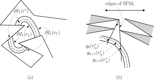
Figure 8: (a) For all $r_{L}\leq r\leq r_{U}$, the combinatorial structures of $\partial I_{1}(r)$ are the same. (b) The points $g_{k}(r_{ij}^{*})$ and $g_{k+2}(r_{ij}^{*})$ are intersections of $\partial I_{1}(r_{ij}^{*})$ and edges of $\mathsf{SPM}_{i}$. The point $g_{k+1}(r_{ij}^{*})$ is an endpoint of a finer arc of $\partial I_{1}(r_{ij}^{*})$.

We compute the farthest-point geodesic Voronoi diagrams, denoted by $\mathsf{FV}_{1}$ and $\mathsf{FV}_{2}$, of the vertices in $C[v_{i+1},v_{j}]$ and $C[v_{j+1},v_{i}]$ in $O(n\log\log n)$ time, respectively, as we did in the decision algorithm (refer to Section 4.1). Let $I_{1}(r)=\cap_{k=i+1}^{j}{D_{r}(v_{k})}$ and $I_{2}(r)=\cap_{k={j+1}}^{i}{D_{r}(v_{k})}$. Instead of computing $\partial I_{1}(r_{ij}^{*})$ and $\partial I_{2}(r_{ij}^{*})$ explicitly, we compute the combinatorial structures of $\partial I_{1}(r_{ij}^{*})$ and $\partial I_{2}(r_{ij}^{*})$. Here, the combinatorial structures of $\partial I_{1}(r_{ij}^{*})$ and $\partial I_{2}(r_{ij}^{*})$ are the cyclic sequences of edges of the farthest-point geodesic Voronoi diagram intersecting $\partial I_{1}(r_{ij}^{*})$ and $\partial I_{2}(r_{ij}^{*})$ in clockwise order, respectively.

For each vertex $v_{f}$ in $\mathsf{FV}_{1}$ and $\mathsf{FV}_{2}$, we compute $d(v_{f},t)$ for all sites $t$ of the cells incident to $v_{f}$. Let $\mathcal{R}$ be the set of these distances. Then we have $|\mathcal{R}|=O(n)$. We sort those distances in increasing order and apply binary search on $\mathcal{R}$ to find the largest value $r_{U}\in\mathcal{R}$ and the smallest values $r_{L}\in\mathcal{R}$ satisfying $r_{ij}^{*}\in[r_{L},r_{U}]$ using the decision algorithm. We have already constructed $\mathsf{FV}_{1}$ and $\mathsf{FV}_{2}$. And we compute $\mathcal{L}_{i}$ and $\mathcal{L}_{j}$, which are independent of $r$. Then the decision algorithm takes linear time. Thus, this procedure takes $O(n\log n)$ time.

Then, for any radius $r\in[r_{L},r_{U}]$, the combinatorial structure of $\partial I_{1}(r)$ is the same. See Figure 8(a). Thus, by computing $\partial I_{1}(r_{L})$, we can obtain the combinatorial structure of $\partial I_{1}(r_{ij}^{*})$. Note that each endpoint of the arcs of $\partial I_{1}(r)$ can be represented as algebraic functions of $r$ with constant degree for $r\in[r_{L},r_{U}]$.

5.2 Subdividing the intersections of geodesic disks

In the following, we let $t$ be $1$ or $2$. We subdivide $\partial I_{t}(r_{ij}^{*})$ by overlaying $\mathsf{SPM}_{i}$, $\mathsf{SPM}_{i+1}$, $\mathsf{SPM}_{j}$, and $\mathsf{SPM}_{j+1}$ with $\partial I_{t}(r_{ij}^{*})$. Instead of computing it explicitly, we compute the combinatorial structure of the subdivision of $\partial I_{t}(r_{ij}^{*})$.

First we compute the shortest path map $\mathsf{SPM}_{i}$. The annulus $I_{t}(r_{U})\setminus\mathrm{int}(I_{t}(r_{L}))$ does not contain any vertex of the shortest path map. Thus the edges of $\mathsf{SPM}_{i}$ intersecting the curve $\partial I_{t}(r)$ can be ordered along the curve $\partial I_{t}(r_{U})$ in clockwise fashion for any $r\in[r_{L},r_{U}]$. Moreover, the order of these edges is the same for any $r\in[r_{L},r_{U}]$. Thus, this order can be computed in linear time by traversing $\partial I_{t}(r_{U})$ and $\mathsf{SPM}_{i}$ as we did in Section 4.3.2. We do this also for $\mathsf{SPM}_{i+1}$, $\mathsf{SPM}_{j}$, and $\mathsf{SPM}_{j+1}$.

Consider an edge $e$ of $\mathsf{SPM}_{i}$ intersecting $\partial I_{t}(r)$ for $r\in[r_{L},r_{U}]$. Then the intersection can be represented as an algebraic function of $r$. We compute such an algebraic function for each edge of $\mathsf{SPM}_{i}$, $\mathsf{SPM}_{i+1}$, $\mathsf{SPM}_{j}$, and $\mathsf{SPM}_{j+1}$ and merge them with the set of the endpoints of the arcs in $\partial I_{t}(r)$ for $r\in[r_{L},r_{U}]$ computed in Section 5.1. Let $\mathcal{A}$ denote the merged set. There are $O(n)$ elements in $\mathcal{A}$ each of which is an algebraic function of the variable $r$. They can be sorted in clockwise order along $\partial I_{t}(r_{ij}^{*})$ in $O(n\log^{2}n)$ time by Lemma 22. See Figure 8. Let $\mathcal{A}=\{g_{1}(r),\ldots,g_{m}(r)\}$. The elements are the endpoints of finer arcs of $\partial I_{t}(r)$. Let $\{g^{\prime}_{1}(r),\ldots,g^{\prime}_{m^{\prime}}(r)\}$ be the sorted list of the endpoints of finer arcs of $\partial I_{2}(r)$ for $r\in[r_{L},r_{U}]$.

Lemma 22

The sorted list $\mathcal{A}$ can be computed in $O(n\log^{2}n)$ time.

Proof.  As described above, we can compute all elements of $\mathcal{A}$ in linear time. In the following, we show that they can be sorted in $O(n\log^{2}n)$ time. Sorting $O(n)$ elements can be done in $O(T_{\textnormal{c}}\log n)$ time using $O(n)$ processors [8], where $T_{\textnormal{c}}$ is the time for comparing two elements. To compare two elements, that is, to determine the order for the two elements along $\partial I_{t}(r_{ij}^{*})$ with respect to the reference point for $\partial I_{t}(r_{ij}^{*})$, we do the followings. Let $h_{1}(r_{ij}^{*})$ and $h_{2}(r_{ij}^{*})$ be two elements of $\mathcal{A}$. Here, $h_{1}(r)$ and $h_{2}(r)$ are algebraic functions of variable $r\in\mathbb{R}$, and we want to determine the order for them when $r=r_{ij}^{*}$. We first find the roots of $h_{1}(r)=h_{2}(r)$. Let $c$ be the number of roots, which is a constant. We apply the decision algorithm $c$ times with the roots. Then we can compare $h_{1}(r_{ij}^{*})$ and $h_{2}(r_{ij}^{*})$ in $O(n)$ time, which is the time for applying the decision algorithm $c$ times. In other words, $T_{\textnormal{c}}=O(n)$ for our case. Note that we have already constructed the farthest-point geodesic Voronoi diagrams.

We apply parametric search [15] with this parallel sorting algorithm. In each iteration of the sorting, we need to do $O(n)$ comparisons, which are done in different processors in the parallel sorting algorithm. That means each of them is independent of the others. Thus, in each iteration, we find $O(n)$ roots for all functions. Then we sort them and apply binary search on $O(n)$ roots using the decision algorithm. Each iteration takes $O(n\log n)$ time, thus the total time complexity is $O(n\log^{2}n)$ time.    

This section can be summarized as follows.

Lemma 23

The set of endpoints of the finer arcs of $\partial I_{1}(r)$ and $\partial I_{2}(r)$ can be computed in $O(n\log^{2}n)$ time for $r\in[r_{L},r_{U}]$.

5.3 Computing the coverage function values

Recall that the function $\phi_{1}(p)$ maps a point $p\in P$ to the infimum of the numbers which represent the points in $D_{r}(p)\cap e_{i}$. We find the subedge that contains $\phi_{1}(g_{k}(r_{ij}^{*}))$ for each index $k\in[1,m]$ in $O(n\log^{2}n)$ time. In the decision algorithm, this can be done in $O(n)$ time. However, each comparison in the decision algorithm depends on the results of the comparisons in the previous steps, thus this algorithm cannot be parallelized. Therefore, we devise an alternative algorithm which can be parallelized by allowing more comparison steps.

Lemma 24

For an index $k\in[1,m]$, the subedge of $e_{i}$ containing $\phi_{1}(g_{k}(r_{ij}^{*}))$ can be computed in $O(n\log n)$ time.

Proof.  For a fixed $r$, we can compute $\phi_{1}(g_{k}(r))$ in $O(\log^{2}n)$ time by Lemma 14. However, since we do not know the exact value $r_{ij}^{*}$, we cannot apply the algorithm of Lemma 14. Instead, we again apply parametric search.

The first step of the algorithm for finding $\phi_{1}(x)$ in Lemma 14 is to compute $d(p_{\mathrm{med}},x)$, where $p_{\mathrm{med}}$ is the median of $\mathcal{L}_{i}$. Since $g_{k}(r)$ is contained in the same cell of $\mathsf{SPM}_{i}$ and in the same cell of $\mathsf{SPM}_{i+1}$ for all $r\in[r_{L},r_{U}]$, the combinatorial structures of $\pi(p_{\mathrm{med}},g_{k}(r))$ are the same for all $r\in[r_{L},r_{U}]$. To determine whether $p_{\mathrm{med}}$ comes before or after $\phi_{1}(g_{k}(r_{ij}^{*}))$ from $v_{i}$ in $\mathcal{L}_{i}$, we check the sign of the value $r_{ij}^{*}-d(p_{\mathrm{med}},g_{k}(r_{ij}^{*}))$. If it is positive, then $p_{\mathrm{med}}$ comes before $\phi_{1}(g_{k}(r_{ij}^{*}))$. If it is negative, then $p_{\mathrm{med}}$ comes after $\phi_{1}(g_{k}(r_{ij}^{*}))$. Otherwise, $p_{\mathrm{med}}$ equals $\phi_{1}(g_{k}(r_{ij}^{*}))$. We compute the roots of $r-d(p_{\mathrm{med}},g_{k}(r))=0$ and apply the decision algorithm in Section 4 to the roots. Since the farthest-point geodesic Voronoi diagrams have already been constructed, the running time for each call of the decision algorithm is $O(n)$. Then we can determine the sign of the value in $O(n)$ time even though we still do not know the exact value $r_{ij}^{*}$.

After repeating this step $O(\log n)$ times, we can finally find the subedge of $e_{i}$ containing $\phi_{1}(g_{k}(r_{ij}^{*}))$ in $O(n\log n)$ time.    

Since the total number of indices is $m=O(n)$, we can compute the subedge of $e_{i}$ containing $\phi_{1}(g_{k}(r_{ij}^{*}))$ for all indices $k\in[1,m]$ in $O(n^{2}\log n)$ time. To compute them efficiently, we parallelize this procedure using $O(n)$ processors. A processor is assigned to each index. In each iteration, we compute the roots of $r-d(p_{k},g_{k}(r))=0$ for all indices $k\in[1,m]$ and sort them, where $p_{k}$ is the median of the current search space of an index $k$. There are $O(n)$ roots. We apply binary search on the roots using our decision algorithm and find the interval that containing $r_{ij}^{*}$. Then in $O(n\log n)$ time, we can finish the comparisons in each iteration as we did in the proof of Lemma 22. We need $O(\log n)$ iterations to find the subedges, so we can compute the subedges for all indices in $O(n\log^{2}n)$ time. We do this also for $\psi_{1}(x)$. Similarly, we compute the subedges containing the function values $\phi_{2}(x),\psi_{2}(x)$ for all endpoints $x$ in $\partial I_{2}(r_{ij}^{*})$ in $O(n\log^{2}n)$ time.

Then, we compute the algebraic functions $\phi_{1}(g_{k}(r))$ and $\phi_{2}(g^{\prime}_{k^{\prime}}(r))$ for all indices $k\in[1,m]$ and all indices $k^{\prime}\in[1,m^{\prime}]$. Then we sort the points in $\mathcal{L}_{i}$ and the points $\phi_{1}(g_{k}(r_{ij}^{*})),\phi_{2}(g^{\prime}_{k^{\prime}}(r_{ij}^{*}))$ for all indices $k\in[1,m]$ and all indices $k^{\prime}\in[1,m^{\prime}]$ in $O(n\log^{2}n)$ time using a way similar to the algorithm in Lemma 22.

Lemma 25

The points $\phi_{1}(g_{k}(r_{ij}^{*}))$ and $\phi_{2}(g^{\prime}_{k^{\prime}}(r_{ij}^{*}))$ for all indices $k\in[1,m]$ and $k^{\prime}\in[1,m^{\prime}]$, and the points in $\mathcal{L}_{i}$ can be sorted in $O(n\log^{2}n)$ time.

5.4 Constructing quadruples consisting of two cells and two subedges

Consider a quadruple $(x_{1},x_{2},y_{1},y_{2})$, where $x_{t}$ is a finer arc of $\partial I_{t}(r_{ij}^{*})$ for $t=1,2$, and $y_{1}$ and $y_{2}$ are subedges in $e_{i}$ and $e_{j}$, respectively. We say the quadruple $(x_{1},x_{2},y_{1},y_{2})$ is optimal if there is a $2$-center $(c_{1},c_{2})$ such that $c_{1}\in x_{1},c_{2}\in x_{2}$ and $\alpha\in y_{1},\beta\in y_{2}$ for some point-partition $(\alpha,\beta)$ with respect to $(c_{1},c_{2},r_{ij}^{*})$. Given an optimal quadruple, we can compute $c_{1}$ and $c_{2}$ in constant time by the following lemma.

Lemma 26

Given an optimal $4$-tuple $(x_{1},x_{2},y_{1},y_{2})$, a $2$-center $(c_{1},c_{2})$ restricted to the candidate edge pair $(e_{i},e_{j})$ can be computed in constant time.

Proof.  Let $(c_{1}^{*},c_{2}^{*})$ be the $2$-center corresponding to the given $4$-tuple. Consider the subdivision $\mathcal{M}_{t}$ which is the overlay of the graph obtained by extending the edges of the shortest path trees rooted at ${v_{i}}$, ${v_{i+1}}$, ${v_{j}}$, ${v_{j+1}}$ in both directions with $\mathsf{FV}_{t}$ for $t=1,2$. (We do not construct $\mathcal{M}_{1}$ and $\mathcal{M}_{2}$ explicitly. We introduce these subdivisions to make it easier to understand the analysis of our algorithm.) By the construction of finer arcs and subedges, $x_{t}$ is contained in a cell of $\mathcal{M}_{t}$ for $t=1,2$. Moreover, each endpoint of a finer arc lies either on an edge of a shortest path map or on an edge of a farthest-point geodesic Voronoi diagram. Let $f_{t}$ be the site of the cell of $\mathsf{FV}_{t}$ containing $x_{t}$. Let $w_{1}^{*},w_{2}^{*},w_{3}^{*}$ and $w_{4}^{*}$ be the points that minimize the following function $g(w_{1},w_{2},w_{3},w_{4})$ for $w_{1}\in x_{1},w_{2}\in x_{2},w_{3}\in y_{1}$, and $w_{4}\in y_{2}$.

$$g(w_{1},w_{2},w_{3},w_{4})=\max\{d(w_{1},f_{1}),d(w_{1},w_{3}),d(w_{1},w_{4}),d(w_{2},f_{2}),d(w_{2},w_{3}),d(w_{2},w_{4})\}$$

Then $(w_{1}^{*},w_{2}^{*})$ is the $2$-center restricted to $(e_{i},e_{j})$.

Since each element of the quadruple is fully contained in some cell of $\mathcal{M}_{1}$ or $\mathcal{M}_{2}$, $g(w_{1},w_{2},w_{3},w_{4})$ is the maximum of the six algebraic functions of constant degree. Thus we can find the minimum of $g(w_{1},w_{2},w_{3},w_{4})$ in constant time.    

However, there are more than quadratic number of such quadruples. Instead of considering all of them, we construct a set of quadruples with size $O(n)$ containing at least one optimal quadruple as follows.

We first compute the event points on $\partial I_{t}(r_{ij}^{*})$. An event point on $\partial I_{t}(r_{ij}^{*})$ is a point $x$ with $d(x,p)=r_{ij}^{*}$ for some point $p\in\mathcal{L}_{i}$. We do not need to compute the exact positions for event points. Instead, we compute their relative positions, i.e., we implicitly maintain those points sorted in clockwise order along $\partial I_{t}(r_{ij}^{*})$. We can do this in $O(n\log^{2}n)$ time as we did in the proof of Lemma 25.

Now we have all the event points that subdivide the chain $\partial I_{1}(r_{ij}^{*})$ and $\partial I_{2}(r_{ij}^{*})$ into $O(n)$ subarcs. Moreover, we have subdivided the edges $e_{i}$ and $e_{j}$ into $O(n)$ subedges (refer to Section 4.4). Then, we construct the set of quadruples $(x_{1},x_{2},y_{1},y_{2})$ such that there are event points $p(r)\in x_{1}$ and $q(r)\in x_{2}$, which are indeed algebraic functions, satisfying $\phi_{1}(p(r_{ij}^{*}))\in y_{1}$, $\psi_{1}(p(r_{ij}^{*}))\in y_{2}$, $\phi_{2}(q(r_{ij}^{*}))\in y_{1}$ and $\psi_{2}(q(r_{ij}^{*}))\in y_{2}$. Note that each event point $p(r)$ lies in the same cell of $\mathcal{M}_{t}$ for all $r\in[r_{L},r_{U}]$ by the construction. Using the information we computed before, we can construct the set of those quadruples in time linear to the size of the set, which is $O(n)$,

Moreover, since we consider all quadruples one of which is an optimal $4$-tuple, we can find a $2$-center restricted to $(e_{i},e_{j})$ using the procedure in this section in $O(n\log^{2}n)$ time. The following lemma and theorem summarize the our result.

Lemma 27

A $2$-center restricted to a candidate edge pair can be computed in $O(n\log^{2}n)$ time.

Theorem 28

For a simple polygon $P$ with $n$ vertices, a $2$-center of $P$ can be computed in $O(n^{2}\log^{2}n)$ time.

References

- [1] Hee-Kap Ahn, Luis Barba, Prosenjit Bose, Jean-Lou De Carufel, Matias Korman, and Eunjin Oh. A linear-time algorithm for the geodesic center of a simple polygon. In 31st International Symposium on Computational Geometry (SoCG 2015), 2015.
- [2] Hee-Kap Ahn, Luis Barba, Prosenjit Bose, Jean-Lou De Carufel, Matias Korman, and Eunjin Oh. A linear-time algorithm for the geodesic center of a simple polygon. Discrete & Computational Geometry, 56(4):836–859, 2016.
- [3] Boris Aronov, Steven Fortune, and Gordon Wilfong. The furthest-site geodesic voronoi diagram. Discrete & Computational Geometry, 9(1):217–255, 1993.
- [4] Tetsuo Asano and Godfried T. Toussaint. Computing geodesic center of a simple polygon. Technical Report SOCS-85.32, McGill University, 1985.
- [5] Magdalene G. Borgelt, Marc Van Kreveld, and Jun Luo. Geodesic disks and clustering in a simple polygon. International Journal of Computational Geometry & Applications, 21(06):595–608, 2011.
- [6] Timothy M. Chan. More planar two-center algorithms. Computational Geometry, 13(3):189–198, 1999.
- [7] Hsien-Chih Chang, Jeff Erickson, and Chao Xu. Detecting weakly simple polygons. In Proceedings of the Twenty-Sixth Annual ACM-SIAM Symposium on Discrete Algorithms (SODA 2015), pages 1655–1670, 2015.
- [8] Richard Cole. Parallel merge sort. SIAM Journal on Computing, 17(4):770–785, 1988.
- [9] Herbert Edelsbrunner and Ernst Peter Mücke. Simulation of simplicity: A technique to cope with degenerate cases in geometric algorithms. ACM Transactions on Graphics, 9(1):66–104, 1990.
- [10] Tomás Feder and Daniel H. Greene. Optimal algorithms for approximate clustering. In Proceedings of 20th ACM Symposium on Theory of Computing (STOC 1988), pages 434–444, 1988.
- [11] Leonidas Guibas, John Hershberger, Daniel Leven, Micha Sharir, and RobertE. Tarjan. Linear-time algorithms for visibility and shortest path problems inside triangulated simple polygons. Algorithmica, 2(1-4):209–233, 1987.
- [12] R.Z. Hwang, R.C.T. Lee, and R.C. Chang. The slab dividing approach to solve the Euclidean -center problem. Algorithmica, 9(1):1–22, 1993.
- [13] A. K. Jain, M. N. Murty, and P. J. Flynn. Data clustering: a review. ACM Computing Surveys, 31(3):264–323, 1999.
- [14] Sung Kwon Kim and Chan-Su Shin. Efficient algorithms for two-center problems for a convex polygon. In Proceedings of the 6th International Computing and Combinatorics Conference (COCOON 2000), pages 299–309, 2000.
- [15] Nimrod Megiddo. Applying parallel computation algorithms in the design of serial algorithms. Journal of ACM, 30(4):852–865, 1983.
- [16] Nimrod Megiddo. Linear-time algorithms for linear programming in and related problems. SIAM J. Comput., 12(4):759–776, 1983.
- [17] Nimrod Megiddo. On the ball spanned by balls. Discrete & Computational Geometry, 4(1):605–610, 1989.
- [18] Eunjin Oh, Luis Barba, and Hee-Kap Ahn. The farthest-point geodesic Voronoi diagram of points on the boundary of a simple polygon. In Proceedings of the 32nd International Symposium on Computational Geometry (SoCG 2016), pages 56:1–56:15, 2016.
- [19] R. Pollack, M. Sharir, and G. Rote. Computing the geodesic center of a simple polygon. Discrete & Computational Geometry, 4(1):611–626, 1989.
- [20] Ivo Vigan. Packing and covering a polygon with geodesic disks, 2013. http://arxiv.org/abs/arXiv:1311.6033.