Optimization of population annealing Monte Carlo for large-scale spin-glass simulations

Abstract

Population annealing Monte Carlo is an efficient sequential algorithm for simulating $k$-local Boolean Hamiltonians. Because of its structure, the algorithm is inherently parallel and therefore well suited for large-scale simulations of computationally hard problems. Here we present various ways of optimizing population annealing Monte Carlo using $2$-local spin-glass Hamiltonians as a case study. We demonstrate how the algorithm can be optimized from an implementation, algorithmic accelerator, as well as scalable parallelization points of view. This makes population annealing Monte Carlo perfectly suited to study other frustrated problems such as pyrochlore lattices, constraint-satisfaction problems, as well as higher-order Hamiltonians commonly found in, e.g., topological color codes.

I Introduction

Monte Carlo algorithms are widely used in many areas of science, engineering, and mathematics. These approaches are of paramount importance for problems where no analytical solutions are possible. For example, the class of Ising-like Hamiltonians can only be solved analytically in few exceptionally rare cases. The vanilla Ising model can only be solved analytically in one, two, as well as infinite space dimensions. A solution in three space dimensions remains to be found to date Ising (1925); Huang (1987). Therefore, simulations are necessary to understand these systems in three space dimensions. The situation is far more dire when more complex interactions—such as $k$-local terms rather than the usual quadratic or $2$-local terms—are used. Similarly, the inclusion of disorder allows for analytical solutions only in the mean-field regime Edwards and Anderson (1975); Parisi (1979); Sherrington and Kirkpatrick (1975); Binder and Young (1986); Stein and Newman (2013). These spin-glass problems, a subset of frustrated and glassy systems, represent the easiest $2$-local Hamiltonian that is computationally extremely hard. A combination of diverging algorithmic timescales (with the size of the input) due to rough energy landscapes and the need for configurational (disorder) averages to compute thermodynamic quantities makes them the perfect benchmark problem to study novel algorithms. Finally, computing ground states of spin glasses on nonplanar graphs is an NP-hard problem where Monte Carlo methods have been known to be efficient heuristics Katzgraber et al. (2005); Wang et al. (2015a); Zhu et al. (2015a) and where only few efficient exact methods exist for small system sizes.

It is therefore of much importance to design or improve efficient algorithms either to save computational effort or have better quality data with the same computational effort when studying these complex systems. Two popular algorithms that are currently in use (for both thermal sampling, as well as optimization) are parallel tempering (PT) Monte Carlo Geyer (1991); Hukushima and Nemoto (1996) and population annealing Monte Carlo (PAMC) Hukushima and Iba (2003); Zhou and Chen (2010); Machta (2010); Wang et al. (2015b).

Although both PT and PAMC are extended ensemble Monte Carlo methods, PAMC is a sequential Monte Carlo algorithm, in contrast to PT, which is a (replica-exchange) Markov-chain Monte Carlo method. PAMC is a population-based Monte Carlo method and thus well suited for implementations on multicore high-performance computing machines. PAMC is similar to simulated annealing Kirkpatrick et al. (1983), however, with an extra resampling step when the temperature is reduced to maintain thermal equilibrium. PT has been intensively optimized and has been to date the work horse in statistical physics and is equally efficient in simulating spin glasses when compared to PAMC Wang et al. (2015b). PAMC, on the other hand, remains a relatively new simulation method. Although careful systematic studies of PAMC Wang et al. (2014, 2015b) exist, and the method has been applied broadly Wang et al. (2015a); Borovský, M. and Weigel, M. and Barash, Lev Yu. and Žukovič, M. (2016); Barash, Lev Yu. and Weigel, M. and Shchur, Lev N. and Janke, W. (2017); Callaham and Machta (2017), little effort has been made to thoroughly optimize the algorithm. Here we focus on this problem and study various approaches to improve the efficiency of PAMC for large-scale simulations. While some approaches improve PAMC, others have little to no effect. Note that related optimization ideas are explored in Ref. Amey and Machta (2018).

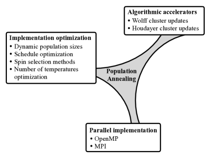
Figure 1: Diagram outlining the different optimizations we have implemented for population annealing Monte Carlo. These range from optimizations in the implementation, such as efficient spin selection techniques, to algorithmic accelerators (e.g., the inclusion of cluster updates), as well as parallel implementations. See the main text for details.

Our strategy to optimize PAMC is three pronged, as illustrated in Fig. 1. First, we study different implementation optimizations. Here we discuss dynamic population sizes that vary with the temperature during the anneal, as well as the optimization of different annealing schedules. We also investigate different spin selection methods (order of spin updates in the simulation) such as random, sequential and checkerboard. While for disordered systems sequential updates are commonplace, random updates are needed for nonequilibrium studies. In the case of bipartite lattices, a checkerboard spin-update technique can be used, which is perfectly suited for parallelization. Furthermore, we discuss how to determine the optimum number of temperatures for a given simulation. Second, we analyze the effects of algorithmic accelerators by adding cluster updates to PAMC. We have studied Wolff cluster updates Wolff (1989), as well as Houdayer cluster updates Houdayer (2001), and isoenergetic cluster moves Zhu et al. (2015a). Third, we discuss different parallel implementations using both OpenMP (ideal for shared-memory machines Wang et al. (2014, 2015b); com (a)) and MPI com (b) with load balancing (ideal for scalable massively parallel implementations). Note that PAMC implemented on graphics processing units has been discussed extensively in Refs. Borovský, M. and Weigel, M. and Barash, Lev Yu. and Žukovič, M. (2016); Barash et al. (2017).

The paper is structured as follows. We first introduce in Sec. II some concepts needed in this study, such as the case study Hamiltonian and outline the PAMC algorithm. Implementation optimizations are presented in Sec. III, algorithmic accelerators via cluster updates in Sec. IV, and parallel implementations are discussed in Sec. V, followed by concluding remarks.

II Preliminaries

In this section we introduce some concepts needed for the PAMC optimization in the subsequent section. In particular, we introduce the Ising spin-glass Hamiltonian (our case study), as well as PAMC and different algorithmic accelerators.

II.1 Case study: Spin glasses

We study the zero-field two-dimensional (2D) and 3D Edwards-Anderson Ising spin glass Edwards and Anderson (1975) given by the Hamiltonian

$$H=-\sum_{\langle ij\rangle}J_{ij}S_{i}S_{j},$$ (1)

where $S_{i}=\pm 1$ are Ising spins and the sum is over the nearest neighbors on a $D$-dimensional lattice of linear size $L$ with $N_{\rm spin}=L^{D}$ spins. The random couplings $J_{ij}$ are chosen from a Gaussian distribution with mean zero and variance $1$. We refer to each disorder realization as an “instance.” The model has no phase transition to a spin-glass phase in 2D Singh and Chakravarty (1986), while in 3D there is a spin-glass phase transition at $T_{\rm c}\approx 0.96$ Katzgraber et al. (2006) for Gaussian disorder.

II.2 Outline of population annealing Monte Carlo

Population annealing Monte Carlo Hukushima and Iba (2003); Zhou and Chen (2010); Machta (2010); Wang et al. (2015b) is similar to simulated annealing (SA) Kirkpatrick et al. (1983) in many ways. For example, both methods are sequential. However, the most important differentiating aspect between PAMC and SA is the addition of a population of replicas that are resampled when the temperature is lowered in the annealing schedule.

PAMC Wang et al. (2015b) starts with a large population of $R$ replicas at a high temperature, where thermalization is easy. In our simulations, we initialize replicas randomly at the inverse temperature $\beta=1/T=0$. The population traverses an annealing schedule with $N_{T}$ temperatures and maintains thermal equilibrium to a low target temperature, $T_{\rm{min}}=1/\beta_{\rm{max}}$. When the temperature is lowered from $\beta$ to $\beta^{\prime}$, the population is resampled. The mean number of the copies of replica $i$ is proportional to the appropriate reweighting factor, $\exp[-(\beta^{\prime}-\beta)E_{i}]$. The constant of proportionality is chosen such that the expectation value of the population size at the new temperature is $R(\beta^{\prime})$. Note that $R(\beta^{\prime})$ is usually kept close to $R$; however, this is not a necessary condition. Indeed, in our dynamical population size implementation, we let $R$ change as a function of $\beta$ and seek better algorithmic efficiency in the number of spin updates. The resampling is followed by $N_{\rm S}=10$ Monte Carlo sweeps (one Monte Carlo sweep represents $N_{\rm spin}$ attempted spin updates) for each replica of the new population using the Metropolis algorithm. We keep $N_{\rm S}=10$ without loss of generality, because the performance of PAMC is mostly sensitive to the product of $N_{\rm S}N_{T}$ near optimum. For example, two PAMC simulations with $\{N_{\rm S}=10,N_{T}\}$ and $\{N_{\rm S}=1,10N_{T}\}$ are similar in efficiency, if $N_{T}$ is reasonably large. The amount of work of a PAMC simulation in terms of sweeps is $W=RN_{\rm S}N_{T}$, where $R$ is the average population size.

As shown in Ref. Wang et al. (2015b), the quality of thermalization of any thermodynamic observable is in direct correlation with the family entropy $S_{\rm f}$ and the entropic family size $\rho_{\rm s}$. The systematic errors, on the other hand, are controlled by the equilibrium population size $\rho_{\rm f}$. What we here refer to as “efficiency” or “speed-up” relates to reducing the statistical as well as the systematic errors while keeping the computational effort constant. Thus, it would be reasonable to use these quantities as measures of optimality for various PAMC implementations. $S_{\rm f}$, $\rho_{\rm s}$, and $\rho_{\rm f}$ are defined as

$$S_{\rm f} = -\sum_{i}\nu_{i}\ln\nu_{i},$$ (2)

$$\rho_{\rm s} = \lim_{R\rightarrow\infty}R/e^{S_{\rm f}},$$ (3)

$$\rho_{\rm f} = \lim_{R\rightarrow\infty}R\times\rm{var}(\beta F),$$ (4)

where $\nu_{i}$ is the fraction of the population that has descended from replica $i$ in the initial population, and $\beta$ and $F$ are the inverse temperature and free energy of the system, respectively. The free energy is measured using the free-energy perturbation method. Intuitively, $\exp(S_{\rm f})$ characterizes the number of surviving families and $\rho_{\rm s}$ the average surviving family size. For a set of simulation parameters, the larger $\rho_{\rm s}$ and $\rho_{\rm f}$, or the smaller $S_{\rm f}$, the computationally harder the instance. Keep in mind that $\rho_{\rm f}$ is computationally more expensive to measure, because many independent runs (at least $10$) are needed to measure the variance of the free energy. Note that $S_{\rm f}$ is “extensive” and asymptotically grows as $\log(R)$, while both $\rho_{\rm s}$ and $\rho_{\rm f}$ are “intensive” quantities, growing asymptotically independent of $R$ when $R$ is sufficiently large. In our simulations, these metrics are estimated using finite but large-enough $R$ values such that the systematic errors are negligible.

It can be shown Wang et al. (2015b); Amey and Machta (2018) that the systematic errors in any population annealing observable at the limit of large $R$ are proportional to ${\rm var}(\beta F)$. Therefore, in order to ensure that the simulations are not affected by the systematic errors, one needs to make certain that the quantity $\rho_{\rm f}/R$ is sufficiently small. When well defined, $\rho_{\rm s}$ is strongly correlated with $\rho_{\rm f}$ Wang et al. (2015b) as it is the case for the majority of the spin-glass instances that we study in this paper. Hence, we may alternatively minimize $\rho_{\rm s}/R$ or equivalently maximize $S_{\rm f}$ as a proxy for the quality of equilibration. In our simulations, we ensure that $S_{\rm f}\gtrsim 2$ for all the instances.

Table 1: Simulation parameters for various experiments to optimize PAMC: Spin selection methods (SSM), annealing schedules (AS), number of temperatures tuning (NT), dynamic population size experiment (DPS), and cluster algorithms (CA). $D$ is the space dimension, $L$ is the linear system size, $R$ is the population size, $T_{\rm{min}}=1/\beta_{\rm{max}}$ is the lowest temperature simulated, $N_{T}$ is the number of temperatures, and $M$ is the number of disorder realizations studied. The label “Schedule” refers to the annealing schedule used, such as the linear-in-$\beta$ (LB) or the linear-in-$\beta$ linear-in-$T$ (LBLT) schedules. $N_{\rm S}=10$ sweeps are applied to each replica at each temperature. Note that in the case of dynamic population sizes (DPS), $R$ is the mean population size. See the text for more details.

Technique	$D$	$L$	$R$	$T_{\rm{min}}$	$N_{T}$	Schedule	$M$
SSM	$3$	$4$	$5\times 10^{4}$	$0.2$	$101$	LB	$1000$
SSM	$3$	$6$	$2\times 10^{5}$	$0.2$	$101$	LB	$1000$
SSM	$3$	$8$	$5\times 10^{5}$	$0.2$	$201$	LB	$1000$
SSM	$3$	$10$	$1\times 10^{6}$	$0.2$	$301$	LB	$1000$
AS	$3$	$8$	$5\times 10^{5}$	$0.2$	$201$	All	$1000$
AS	$3$	$10$	$1\times 10^{6}$	$0.2$	$301$	All	$1000$
NT	$2$	$8$	$5\times 10^{4}$	$0.2$	variable	LBLT	$100$
NT	$2$	$16$	$2\times 10^{5}$	$0.2$	variable	LBLT	$100$
NT	$2$	$25$	$5\times 10^{5}$	$0.2$	variable	LBLT	$100$
NT	$2$	$32$	$1\times 10^{6}$	$0.2$	variable	LBLT	$100$
NT	$3$	$4$	$5\times 10^{4}$	$0.2$	variable	LBLT	$100$
NT	$3$	$6$	$2\times 10^{5}$	$0.2$	variable	LBLT	$100$
NT	$3$	$8$	$5\times 10^{5}$	$0.2$	variable	LBLT	$100$
NT	$3$	$10$	$1\times 10^{6}$	$0.2$	variable	LBLT	$100$
DPS	$3$	$6$	$2\times 10^{5}$	$0.2$	$101$	LB	$1000$
DPS	$3$	$8$	$5\times 10^{5}$	$0.2$	$201$	LB	$1000$
DPS	$3$	$10$	$1\times 10^{6}$	$0.2$	$301$	LB	$1000$
CA	$2$	$8$	$5\times 10^{4}$	$0.2$	$101$	LB/LBLT	$1000$
CA	$2$	$16$	$2\times 10^{5}$	$0.2$	$101$	LB/LBLT	$1000$
CA	$2$	$25$	$5\times 10^{5}$	$0.2$	$201$	LB/LBLT	$1000$
CA	$2$	$32$	$1\times 10^{6}$	$0.2$	$301$	LB/LBLT	$1000$
CA	$3$	$4$	$5\times 10^{4}$	$0.2$	$101$	LB/LBLT	$1000$
CA	$3$	$6$	$2\times 10^{5}$	$0.2$	$101$	LB/LBLT	$1000$
CA	$3$	$8$	$5\times 10^{5}$	$0.2$	$201$	LB/LBLT	$1000$
CA	$3$	$10$	$1\times 10^{6}$	$0.2$	$301$	LB/LBLT	$1000$

II.3 Outline of cluster updates used

Having outlined PAMC, we now briefly introduce the different cluster algorithms we have experimented with in order to speed up thermalization.

II.3.1 Wolff cluster algorithm

The Wolff algorithm Wolff (1989) greatly speeds up simulations of Ising systems without frustration near the critical point. It is well known that the Wolff algorithm does not work well for spin glasses in 3D Kessler and Bretz (1990) because the cluster size grows too quickly with $\beta$. Nevertheless, we revisit this algorithm systematically in both 2D and 3D. The idea is that even if the cluster size grows too quickly when $\beta$ is still relatively small, the mean cluster size (normalized by the number of spins $N_{\rm spins}$) is still a continuous function in the range $[0,1]$ when $\beta$ grows from $\beta=0$ to $\infty$. Therefore, it is a reasonable question to ask if there would be some speed-up when restricting the algorithm to the temperature range where the normalized mean cluster size is neither too larger nor too small, for example, in the range $[0.1,0.9]$.

In the ferromagnetic Ising model, where $J_{ij}=J=1$, one adds a neighboring spin $S_{j}$ when it is parallel to a spin $S_{i}$ in the cluster with probability $p_{\rm{c}}=1-\exp(-2J\beta)$. In spin glasses, this is generalized as follows: One adds a neighboring spin $S_{j}$ to $S_{i}$ when the bond between the two spins is satisfied and with probability $p_{\rm{c}}=1-\exp(-2|J_{ij}|\beta)$. This can be compactly written as $p_{\rm{c}}=\max[0,1-\exp(-2\beta J_{ij}S_{i}S_{j})]$ Kessler and Bretz (1990). Note that from $p_{\rm{c}}$, there are two interesting limits for the mean cluster size. In the limit $\beta\rightarrow 0$, the average cluster size is clearly $0$, and in the limit $\beta\rightarrow\infty$, the normalized cluster size tends to $1$, because in the ground state each spin has at least one satisfied bond with its neighbors and all the spins would be added to the cluster. From the expression for $p_{\rm{c}}$ one can see that frustration actually makes the cluster size grow slower as a function of $\beta$. However, frustration also significantly reduces the transition temperature, which is the primary reason why the Wolff algorithm is less efficient for spin glasses. Finally, note that the Wolff algorithm is both ergodic and satisfies detailed balance.

II.3.2 Houdayer cluster algorithm

Designed for spin glasses, the Houdayer cluster algorithm Houdayer (2001) or its generalization, the isoenergetic cluster moves (ICM) Zhu et al. (2015b), greatly improves the sampling for parallel tempering in 2D, while less so in 3D. ICM in 3D, like the Wolff algorithm, is restricted to a temperature window where the method is most efficient Zhu et al. (2015b). ICM works by updating two replicas at the same time. First, an overlap between the two replicas is constructed, which naturally forms positive and negative islands. One island is selected, and the spin configurations of the island in both replicas are flipped.

In its original implementation, the spin down sector is always used to construct the cluster. In the implementation of Zhu et al. a full replica is flipped if the chosen island is in the positive sector to make it negative Zhu et al. (2015b) and therefore reduce the size of the clusters. Here, we improve on this implementation by allowing the chosen island to be either positive or negative, and flipping the spins of the island in both replicas. Therefore, we never flip a full replica. This saves computational time and also has the advantage that it does not artificially make the spin overlap function symmetric. ICM satisfies detailed balance but is not ergodic. Therefore, the algorithm is usually combined with an ergodic method such as the Metropolis algorithm. ICM greatly improves the thermalization time, and also slightly improves the autocorrelation time in parallel tempering. Because PAMC is a sequential method, there is no thermalization stage. We therefore focus on whether the algorithm reduces correlations, i.e., systematic and statistical errors. Our implementation of PAMC with ICM is as follows: First, after each resampling step, we do regular Monte Carlo sweeps and ICM updates alternately. We first do $N_{\rm S}/2$ lattice sweeps for each replica, followed by $R$ ICM updates done by randomly pairing two replicas in the population, followed by another $N_{\rm S}/2$ lattice sweeps. Second, for each ICM update, we choose an island from the spin sector with the smaller number of spins. Then the spin configurations of the island in both replicas are flipped. This effectively means that the spin configurations associated with the selected island are either exchanged or flipped depending on the sign of the island being negative in the former or positive in the latter. Note that the combined energy of the two replicas is conserved in both cases, therefore making the algorithm rejection free.

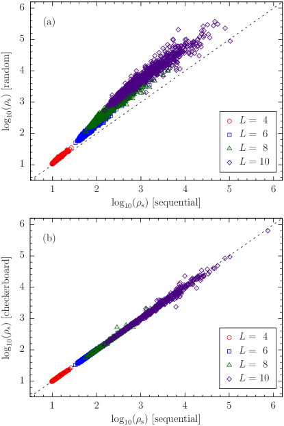
Figure 2: Comparison of the entropic population size $\rho_{\rm s}$ for different spin selection methods: random, sequential and checkerboard updates in three space dimensions. Sequential and checkerboard updates have similar efficiency (b), and both are more efficient than random updates (a).

III Implementation optimizations

In this section, we present our implementation improvement to the population annealing algorithm. We first present spin selection methods, followed by experiments using different annealing schedules, numbers of temperatures, and the use of a dynamic population. The simulation parameters are summarized in Table 1.

III.1 Comparison of spin selection methods

We have studied three spin selection methods: sequential, random, and checkerboard. We have carried out a large-scale simulation in 3D to compare these methods for $L=4$, $6$, $8$, and $10$, with $1000$ instances for each system size. We first run the simulations using the parameters in Table 1. To measure $S_{\rm f}$ or $\rho_{\rm s}$ reliably, we require $S_{\rm f}\gtrsim 2$ Wang et al. (2015b). When this is not satisfied for a particular instance, we rerun it with a larger population size. We then compare $\rho_{\rm s}$ at the lowest temperature between different spin selection methods. Figure 2 shows scatter plots comparing $\rho_{\rm s}$ instance by instance for different system sizes and using different spin selections methods. Figure 2(a) compares random to sequential updates, whereas Fig. 2(b) compares checkerboard to sequential updates. Interestingly, sequential and checkerboard updates have similar efficiency (the data lie on the diagonal), whereas both sequential and checkerboard are more efficient than random updates. This is particularly visible for the larger system sizes, e.g., $L=10$. The random selection method is therefore the least efficient update technique for disordered Boolean problems, keeping in mind that it requires the computation of an additional random number for each attempted spin update thus slowing down the simulation. We surmise that a sequential updating of the spins accelerates the mobility of domain walls in most cases. However, in some pathological examples, such as the one-dimensional Ising chain random updating is needed for Monte Carlo to be ergodic.

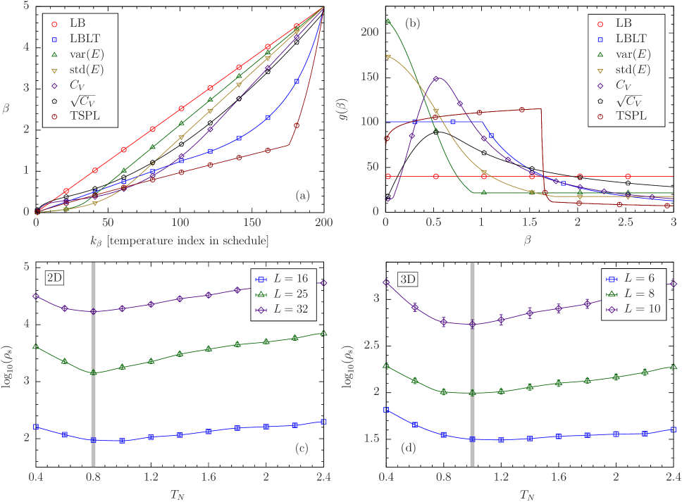
Figure 3: Panel (a) shows the $\beta$ values as a function of the inverse temperature index $k_{\beta}$ for the different schedules experimented with and panel (b) shows the resulting $\beta$ densities $g(\beta)$ (the data are cut off at $\beta=3$ for clarity). Note that both TSPL and LBLT schedules have more temperatures at high $T$. Panels (c) and (d) show $\rho_{\rm s}$ as a function of $T_{N}$ for 2D and 3D simulations, respectively. The vertical shaded line marks the optimum. See the main text for details.

III.2 Optimizing annealing schedules

Most early population annealing simulations used a simple linear-in-$\beta$ (LB) schedule where the change in $\beta$ in the annealing schedule is constant as a function of the temperature index. This, however, is not necessarily the most optimal schedule to use. We use two approaches to optimize the annealing schedules and the number of temperatures: One approach uses a mathematical model with free parameters to be optimized and the other includes adaptive schedules based on a guiding function, e.g., the energy fluctuations or the specific heat. For the parametric schedules we introduce a linear-in-$\beta$ linear-in-$T$ (LBLT) and a two-stage power-law schedule (TSPL). For the LBLT schedule there is one parameter to tune, namely a tuning temperature $T_{N}$ com (c). In this schedule, half of the temperatures above $T_{N}$ are linear in $\beta$, while the other half below $T_{N}$ are linear in $T$. For the TSPL schedule we define a rescaled annealing time $\tau=k_{\beta}/(N_{T}-1)\in[0,1]$, where $k_{\beta}$ is the annealing step (or temperature index) $0$, …, $N_{T}-1$. The TSPL schedule is modeled as

$$\beta(\tau)=a\tau^{\alpha_{1}}\theta(\tau_{0}-\tau)+b\tau^{\alpha_{2}}\theta(\tau-\tau_{0}),$$ (5)

where $\theta$ is the Heaviside step function. Here $\alpha_{1}$ and $\alpha_{2}$ are free parameters. $a$ and $b$ enforce continuity and the final annealing temperature. $\tau_{0}$ is selected to enforce a switch-over temperature $\beta_{0}$. We optimize the LBLT schedule with a simple scan of the parameter $T_{N}$. The optimum value of $T_{N}$ (where $\rho_{\rm s}$ is minimal) is shown in Fig. 3(c) for 2D ($T_{N}\approx 0.8$, marked with a vertical shaded area) and Fig. 3(d) for 3D ($T_{N}\approx 1.0$, marked with a vertical shaded area).

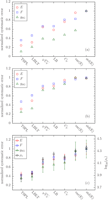
Figure 4: Comparison of the systematic errors for various annealing schedules. The studied observables are energy ($E$), free energy ($F$), and the spin glass Binder cumulant ($g_{\rm SG}$) for the system size $L=10$. Panels (a) and (b) show the systemic errors for two randomly chosen hard instances, whereas panel (c) illustrates the systematic errors averaged over 100 of the hardest instances. Systematic errors of different observable often have magnitudes largely apart. For this reason, the errors in each observable have been normalized relative to the maximum error across all schedules. For instance, in the top panel the ${\rm std}(E)$ schedule which has the greatest systematic error is normalized to 1 while the rest of the schedules lie below 1. It is seen from the plots that the TSPL schedule is the most efficient. The LBLT schedule, although conveniently simple, competes well with the optimal schedule. Note that we also show $\rho_{s}$ (as a dual $y$-axis) in panel (c). We observe that $\rho_{s}$ greatly correlates with the systematic errors justifying the use of it as an effective optimization criterion.

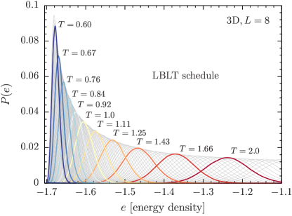
Figure 5: Energy density distribution of the LBLT annealing schedule for $L=8$ in three space dimensions. Thinner curves show the histograms at all temperatures whereas the thicker ones are drawn at every $10$ temperature steps. There are $200$ temperature steps in total. The histograms overlap considerably.

The TSPL schedule, however, has more parameters that have to be tuned. Therefore, we have used the Bayesian optimization package Spearmint Snoek et al. (2012); Adams et al. (2016) rather than a full grid scan in the entire parameter space. We find numerically that the parameters $\alpha_{1}=\exp(-0.0734)$, $\alpha_{2}=\exp(2.15)$, and $\beta_{0}=1.63$ work well. However, we note that there is no guarantee of global optimality. For the adaptive schedules, we optimize using information provided by energy fluctuations, because energy is directly related to the resampling of the population. We therefore define a density of inverse temperature $\beta$, $g(\beta)$, and study the following adaptive schemes.

1. var($E$) schedule with $g(\beta)\sim{\rm{var}}(E)$,

2. std($E$) schedule with $g(\beta)\sim\sqrt{\rm{var}(E)}$,

3. $C_{V}$ schedule with $g(\beta)\sim C_{V}(\beta)$,

4. $\sqrt{C_{V}}$ schedule with $g(\beta)\sim\sqrt{C_{V}(\beta)}$,

where $C_{V}$ is the specific heat of the system. Note that the functions are disorder averaged, and the proportionality is determined by the number of temperatures. Because $g(\beta)$ may become extremely small, we have replaced all the function values that are less than $10\%$ of $\max(g)$ by $0.1\times\max(g)$ to prevent large temperature leaps. With this small modification, we generate $N_{T}$ temperatures according to the above density functions. The shapes and $\beta$ densities of all schedules are shown in Figs. 3(a) and 3(b), respectively. There are clear differences between the different schedules, especially in comparison to the traditionally used LB schedule. We compare the efficiency of these different schedules in Fig. 4 by analyzing the systematic errors in a number of paradigmatic observables. We have studied the internal energy ($E$), free energy ($F$), and the spin-glass Binder cumulant Binder (1981) for the system size $L=10$. To overcome the scale difference when showing the systematic errors for these observables in one plot, we have normalized the errors with respect to the schedule that has the greatest error. Therefore, all the errors will be relative to that of the worst schedule. In Figs. 4(a) and 4(b) we show the normalized systematic errors for two randomly chosen and extremely hard instances. In Fig. 4(c) we show the disorder averaged systematic errors calculated from $100$ of the hardest instances. It can be readily seen from the plots that the LBLT and TSPL schedules yield the best efficiencies among all the experimented schedules with TSPL slightly more efficient. Both LBLT and TSPL schedules place more temperatures at high temperature values (smaller $\beta$ values), presumably because the Metropolis dynamics is more effective at high temperatures. Additionally, in Fig. 4(c) we have shown $\rho_{s}$ for various schedules. We observe great correlation between $\rho_{s}$ and the systematic errors which corroborates the use of $\rho_{s}$ as a good measure of efficiency.

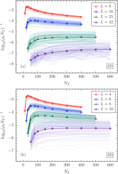
Figure 6: Optimization of the number of annealing steps $N_{T}$ in two space dimensions [2D, panel (a)] and three space dimensions [3D, panel (b)]. To maximize sampling efficiency, one needs to optimize $1/(\rho_{\rm s}N_{T})$ with respect to $N_{T}$. In both panels the points and the solid curves show the disorder average while the dashed envelopes display all $100$ studied instances. For smaller system sizes the peak (optimum) is sharp, whereas for systems with more than approximately $1000$ spins the peak is broadened, especially in two dimensions. The reason for this broadening can be understood by noticing the increase in the density of chaotic samples as the system grows in size (wiggly lines).

We stress that the optimum schedule depends on the choice of the number of sweeps at each anneal step $N_{\rm S}$, because $N_{T}$ and $N_{\rm S}$ are exchangeable when $N_{T}$ is large enough. In our approach, we have fixed $N_{\rm S}$. It is therefore possible that other techniques may result in different optimal schedules. For instance, one may use the energy distribution overlaps at two temperatures to define the optimum schedule Amey and Machta (2018); Barash et al. (2017), which only depends on the thermodynamic properties of the system. As an example, in Fig. 5 we show the energy distributions of the LBLT schedule for $L=8$ in 3D. The energy histograms overlap considerably up to several temperature steps. Within this framework, the optimization is transferred to the distribution of sweeps. However, the density of work (the product of density of $\beta$ and density of sweeps) should be similar in the two different approaches. In our implementation as the number of sweeps is constant, the density of work is the same as the density of $\beta$.

III.3 Optimization of the number of temperatures

To optimize the number of temperatures and their range, we use the LBLT schedule as it is easy to implement and very close to optimal. Our figure of merit is to maximize the number of independent measurements $R/\rho_{\rm s}$ for constant work $W=RN_{\rm S}N_{T}$. We define efficiency as $\gamma=R/(\rho_{\rm s}W)$ by tuning $N_{T}$ for a constant $W$. Because $N_{\rm S}=10$ is fixed, we need to maximize $1/(\rho_{\rm s}N_{T})$ by tuning $N_{T}$. In the limit $R\rightarrow\infty$, $\rho_{\rm s}$ and the efficiency $\gamma$ are independent of the population size. This is expected as $\gamma$ is an intensive quantity. Therefore, to measure $\gamma$, we only need to make sure $R$ is sufficiently large such that $\rho_{\rm s}$ has converged. It is not necessary to use the same $W$ for different $N_{T}$.

The results for both two- and three-dimensional systems are shown in Figs. 6(a) and 6(b), respectively. The solid curves show the disorder average while the dashed envelopes are the instance-by-instance results. It is interesting to note that for relatively smaller system sizes we observe a pronounced peak. The existence of an optimum number of temperatures can be intuitively understood in the following way: For a fixed amount of computational effort, if $N_{T}$ is too small, then the annealing or resampling would become too stochastic, which is inefficient. On the other hand, if the annealing is too slow ($N_{T}$ is too large) this becomes unnecessary and keeping a larger population size is more efficient. Therefore, the optimum comes from a careful balance between $N_{T}$ and $R$. However as the system size grows, the optimum peak starts to flatten out due to the onset of temperature chaos Ney-Nifle and Young (1997); Aspelmeier et al. (2002); Jönsson et al. (2002); Katzgraber and Krzakala (2007); Fernandez et al. (2013); Wang et al. (2015c); Zhu et al. (2016). This can be seen in Fig. 6 as a discernible increase in the density of instances with irregular oscillatory behavior. Thus we conclude that the optimization presented here, although capturing the bulk of the instances, might not be reliable in case of extremely hard (chaotic) instances. Instead one may consider performing more Metropolis sweeps rather than merely increasing the temperature steps or the population size. This is especially relevant if memory (which correlates to $R$) becomes a concern for the hardest instances.

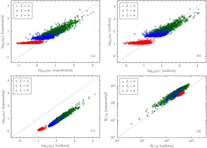
Figure 7: Instance-by-instance comparison for a PAMC simulation with fixed and dynamic population sizes. With a dynamic population size, $\rho_{\rm s}$ and $\rho_{\rm f}$ are well correlated, similarly to the case of uniform population. $\rho_{\rm s}$ is greatly reduced, suggesting that the simulation is much better at the level of averaging over all temperatures. The dynamic population size is also more efficient than the uniform one using the worst-case measure. Here $R_{\rm f}$ is the final population size.

III.4 Dynamic population sizes

The reason the LBLT schedule is more efficient than a simple LB schedule is because the Metropolis dynamics is less effective at low temperatures, and therefore using more “hotter” temperatures is more efficient. Here we investigate another technique, namely a variable number of replicas that depends on the annealing temperature, thus having a similar effect to having more temperatures at higher values. Regular PAMC is designed to have an approximately uniform population size as a function of temperature. Here we allow the population size to change with $\beta$. Because most families are removed at a relatively early stage of the anneal, transferring some replicas from low temperatures to high temperatures may increase the diversity of the final population, even though the final population size would be smaller com (d).

We study a simple clipped exponential population schedule where the population starts as a constant $R_{0}$ until $\beta=\beta_{0}$, and then decreases exponentially to $R_{\rm f}=R_{0}/r$ at $\beta=\beta_{\rm{max}}$,

$$R(\beta)=\begin{cases}R_{0}&\!\!\!\beta\leq\beta_{0}\\ aR_{0}/\left[(r-1)(e^{\beta S}-e^{\beta_{0}S})+a\right]&\!\!\!\beta>\beta_{0},\end{cases}$$ (6)

where $a=\exp(\beta_{\rm{max}}S)-\exp(\beta_{0}S)$. The free parameters to tune are $S$, $\beta_{0}$, and $r$. $S$ is chosen such that the function is continuous and naturally characterizes the slope of the curve. Once the parameters are optimized, we can scale the full function to have a comparable average population size to that of the uniform schedule. The optimization is again done using Bayesian statistics, and we obtain $\beta_{0}=0.9$, $r=33.8$, and $S=\exp(-2.52)$.

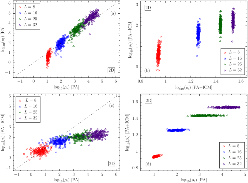
Figure 8: Population annealing with ICM updates in 2D. Note that replica family is not well defined when ICM updates are included. Therefore, we use $\rho_{\rm f}$ to characterize speed-up. Significant speed-up is observed in 2D.

It is noteworthy to mention that there are two different measures to detect efficiency when the population size is allowed to change. For the same average population size, the dynamic population schedule is always better at high temperature. However, at low temperature, a smaller $\rho_{\rm s}$ does not justify that the number of independent measurements is larger, because $R$ is also smaller. It is thus reasonable to optimize the parameters using $\rho_{\rm s}$, and then also to compare to $R/\rho_{\rm s}$. Note that we use the local population size $R$ at each temperature to compute $\rho_{\rm s}$. The correlations and comparisons of $\rho_{\rm s}$ and $\rho_{\rm f}$ are also studied. With the optimum parameters, we compare the efficiency of the dynamic and uniform population sizes. The results are shown in Fig. 7. We see that $\rho_{\rm s}$ and $\rho_{\rm f}$ are well correlated for the dynamic population size. $\rho_{\rm s}$ is greatly reduced, suggesting that the simulation is much better at the level of averaging over all temperatures. We also see that even using the worst-case measure, the dynamic population size is more efficient than the uniform one. Note, however, that the peak memory use of the dynamic population size is larger due to the nonuniformity of the number of replicas as a function of $\beta$.

IV Algorithmic accelerators

We now turn our attention to algorithmic accelerators by including cluster updates in the simulation. The simulation parameters are summarized in Table 1.

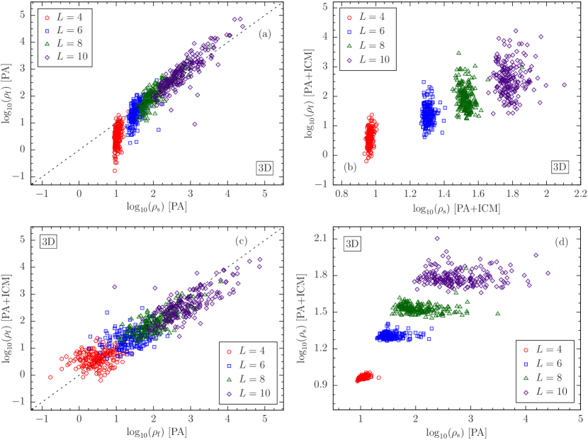
Figure 9: Population annealing with ICM updates in 3D. Note that replica family is not well defined when ICM updates are included. Therefore, we use $\rho_{\rm f}$ to characterize speed-up. Modest speed-up is observed in 3D.

IV.1 Isoenergetic cluster updates

Here we study PAMC with ICM updates. In 3D, similarly to the Wolff algorithm, there is an effective temperature range where ICM (see Ref. Zhu et al. (2015b) for more details) is efficient. In ICM, two replicas are updated simultaneously. This process uses the detailed structure of the two replica configurations, and it is natural to question if the family of a replica is still well defined. For example, occasionally, two replicas may merely exchange their configurations. This is equivalent to exchanging their family names which potentially increases the diversity of the population at little cost. To resolve and investigate this issue, we have therefore measured the (computationally more expensive) equilibration population size $\rho_{\rm f}$ as well, which unlike $\rho_{\rm s}$, does not depend on the definition of the families. Our results are shown in Fig. 8 and Fig. 9, for 2D and 3D, respectively. We find that $\rho_{\rm s}$ is indeed artificially reduced by the cluster updates. In both 2D and 3D, $\rho_{\rm f}$ has a wide distribution, while $\rho_{\rm s}$ is almost identical for all instances. Furthermore, $\rho_{\rm s}$ and $\rho_{\rm f}$ are strongly correlated for regular PAMC, but the correlation is poor when ICM is turned on. Therefore, we conclude that $\rho_{\rm s}$ is no longer a good equilibration metric for PAMC when combined with ICM. Using $\rho_{\rm f}$, we find that similar to PT Zhu et al. (2015b), there is clear speed-up in 2D. In 3D, however, the speed-up becomes again marginal. This is in contrast to the discernible speed-up for PT with the inclusion of ICM in 3D. The results suggest that ICM is mostly efficient in 2D and likely quasi-2D lattices, reducing both thermalization times (PT) and correlations (PAMC and PT). In 3D, ICM merely reduces thermalization times, while marginally influencing correlations.

IV.2 Wolff cluster updates

Wolff cluster updates are not effective in spin-glass simulations. We, nevertheless, have revisited this type of cluster update in the context of PAMC for the sake of completeness. More details can be found in Appendix A.

V Parallel Implementation

Population annealing is especially well suited for parallel computing because operations on the replicas can be carried out independently and communication is minimal. Since OpenMP is a shared-memory parallelization library, it is limited to the resources available on a single node of a high-performance computing system. Although modern compute nodes have many cores and large amounts of RAM, these are considerably smaller than the number of available nodes by often several orders of magnitude. To benefit from machines with multiple compute nodes and therefore simulate larger problem sizes, we now present an MPI implementation of PAMC which can utilize resources up to the size of the cluster. While for typical problem sizes single-node OpenMP implementations might suffice for the bulk of the studied instances, hard-to-thermalize instances could then be simulated using a massively parallel MPI implementation with extremely large population sizes. Although the exact run time depends on many variables such as the simulation parameters, architecture, code optimality, compiler, etc., here we show some example of a typical simulation time with the parameters listed in Table 1. On a 20-core node with Intel Xeon E5-2670 v2 2.50 GHz processors, it takes approximately $1.3$, $12$, and $75$ minutes to simulate an instance in 3D with $N=216$, $512$, and $1000$ spins, respectively.

V.1 Massively parallel MPI implementation

The performance and scaling of our MPI implementation for 3D Edwards-Anderson spin glasses is shown in Fig. 10. Note that the wall time scales $\sim 1/N$ with $N$ the number of cores for less than $1000$ cores. In our implementation, the population is partitioned equally between MPI processes (ranks). Each rank is assigned an index $k$ with I/O operations occurring on the 0th rank. A rank has a local population on which the Monte Carlo sweeps and resampling are carried out. We also define a global index $G$ which is the index of a replica as if it were in a single continuous array. In practice, the global index $G$ of a replica $j$ on a rank $k$ is computed as the sum of the local populations $r_{i}$ on the preceding ranks plus the local index $j$, i.e.,

$$G=j+\sum\limits_{i=0}^{k-1}r_{i}.$$ (7)

The global index for a particular replica varies as its position in the global population changes.

Load balancing is carried out when a threshold percentage between the minimum and maximum local populations is exceeded. In our implementation, all members of a family must be in a continuous range of global indices to allow for efficient computation of the family entropy and the overlap function of the replicas. Therefore, load balancing must maintain adjacency. The destination rank $k$ of a replica is determined by evenly partitioning the global population such that each rank has approximately the same number of replicas, i.e.,

$$k=\lfloor G/\left(\tfrac{R}{N}\right)\rfloor,$$ (8)

where $N$ is the number of ranks (cores).

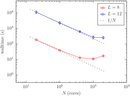
Figure 10: Scaling of the total wall time as a function of the number of processors $N$ for two system sizes $L=8$ and $L=12$. Launching and initialization time are not included. Note that the efficiency becomes better for larger and harder problems. For $L=12$, the scaling remains $1/N$ up to about 1000 processors. The efficiency then decreases when the time for collecting observables becomes dominant. Note that resampling still takes a relatively small time.

Measurement of most observables is typically an efficient accumulation operation, i.e.,

$$\langle\mathcal{A}\rangle=\frac{1}{R}\sum\limits_{k}^{N}\sum\limits_{j}^{r_{k}}\mathcal{A}_{j,k}.$$ (9)

On the other hand, measuring observables such as the spin-glass overlap is more difficult and only done at select temperatures. Sets of replicas are randomly sampled from a rank’s local population and copies are sent to the range of ranks $[(k+N/4)\mod N,(k+3N/4)\mod N]$ with periodic boundary conditions to ensure that the overlap is not computed between correlated replicas. The resulting histograms are merged in an accumulation operation similar to regular observables.

Improving scaling with process count will require a lower overhead implementation of the spin overlap measurements—a problem we intend to tackle in the near future.

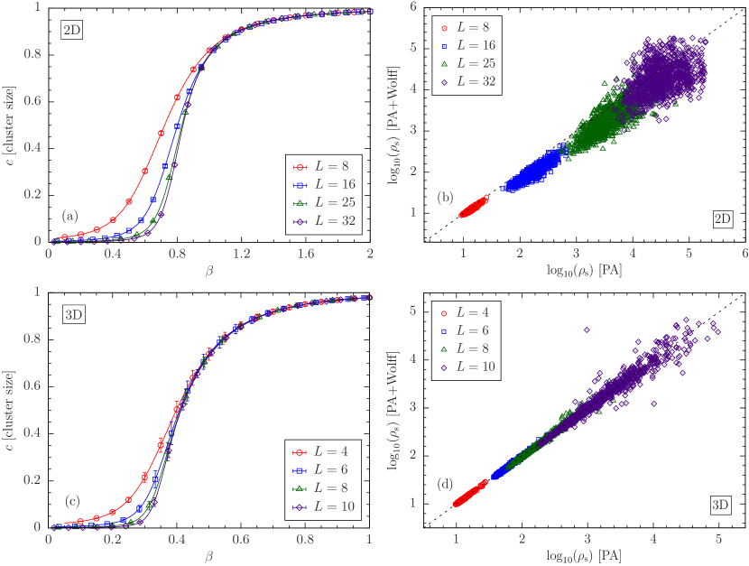
Figure 11: Mean normalized cluster size as a function of $\beta$ for the Wolff algorithm [(a) and (c)] as well as the performance of the algorithm in both 2D and 3D. There is marginal speed-up in 2D (b) and no discernible speed-up in 3D (d).

VI Conclusions and future challenges

We have investigated various ways to optimize PAMC, ranging from optimizations in the implementation, to the addition of accelerators, as well as massively parallel implementations. Many of these optimizations lead to often considerable speed-ups. We do emphasize that these approaches and even the ones that showed only marginal performance improvements for spin glasses in 2D and 3D might be applied to other approaches to simulate statistical physics problems potentially generating sizable performance boosts. The reduction in thermal error studied in this work can most directly be applied to the study of spin glasses by providing more CPU time for disorder averaging.

For the study of spin glasses, our results show that the best performance for PAMC is obtained by selecting the spins in a fixed order, i.e., sequentially or from a checkerboard pattern. Similarly, LBLT and TSPL schedules yield the best performance with LBLT having the least parameters to tune and thus easier to implement. The number of temperatures needed for annealing is remarkably robust for large system sizes. Hence, in order to tackle hard instances, it is often convenient to increase the number of sweeps rather than merely using more temperatures. Dynamic population sizes are desirable, albeit at the cost of a larger memory footprint. However, this can be easily mitigated via massively parallel MPI implementations. In conjunction with Ref. Amey and Machta (2018), and as far as we know, this study represents the first analysis of PAMC from an implementation point of view.

Recently, we learned com (e) that the equilibration population size $\rho_{\rm f}$ can be measured in a single run using a blocking method. It would be interesting to further investigate and test this idea thoroughly in the future. With an optimized PAMC implementation, it would be interesting to also perform large-scale spin-glass simulations to answer some of the unresolved problems in the field, such as the nature of the spin-glass state in three and four dimensions. We plan to address these problems in the near future.

Appendix A Wolff cluster updates

For the Wolff algorithm, we first measure the mean cluster size per spin, as shown in Figs. 11(a) and 11(c) for the 2D and 3D cases, respectively. Note the smooth transition of the mean cluster size from $0$ to $1$. We identify a temperature range where the mean cluster size is in the window $[0.1,0.9]$ com (f). We perform Wolff updates in this temperature range, i.e., we perform $10$ Wolff updates in addition to the $10$ regular Metropolis lattice sweeps for each replica. The comparison of $\rho_{\rm s}$ with regular PAMC is shown in Figs. 11(b) and 11(d). While the Wolff algorithm speeds up ferromagnetic Ising model simulations in 2D, the speed-up is marginal for 2D spin glasses because of the zero-temperature phase transition. In 3D, the Gaussian spin glass has a phase transition near $T_{\rm c}\approx 0.96$, but the temperature window where the Wolff algorithm is effective is much higher than $T_{\rm c}$. The speed-up is therefore almost entirely eliminated, presumably because the Metropolis algorithm is already sufficient for these high temperatures. The fact that the Wolff algorithm is more efficient in 2D than 3D is because clusters percolate faster in 3D, again rendering the effective temperature range higher in 3D. Therefore, Wolff updates constitute unnecessary overhead in the simulation of spin glasses in conjunction with PAMC.

Even though PAMC with the Wolff algorithm does not appear to work very well for spin glasses, this does not mean they cannot be used together. For example, in two-dimensional spin glasses, adding the Wolff algorithm still has marginal benefits. The combination of PAMC and the Wolff cluster updates can be used for ferromagnetic Ising models for the purpose of parallel computing, because parallelizing the Wolff algorithm while doable, is challenging. In population annealing, however, this can be easily parallelized at the level of replicas, and not within the Wolff algorithm itself.

References

- Ising (1925) E. Ising, Beitrag zur Theorie des Ferromagnetismus, Z. Phys. 31, 253 (1925).
- Huang (1987) K. Huang, Statistical Mechanics (Wiley, New York, 1987).
- Edwards and Anderson (1975) S. F. Edwards and P. W. Anderson, Theory of spin glasses, J. Phys. F: Met. Phys. 5, 965 (1975).
- Parisi (1979) G. Parisi, Infinite number of order parameters for spin-glasses, Phys. Rev. Lett. 43, 1754 (1979).
- Sherrington and Kirkpatrick (1975) D. Sherrington and S. Kirkpatrick, Solvable model of a spin glass, Phys. Rev. Lett. 35, 1792 (1975).
- Binder and Young (1986) K. Binder and A. P. Young, Spin Glasses: Experimental Facts, Theoretical Concepts and Open Questions, Rev. Mod. Phys. 58, 801 (1986).
- Stein and Newman (2013) D. L. Stein and C. M. Newman, Spin Glasses and Complexity, Primers in Complex Systems (Princeton University Press, Princeton NJ, 2013).
- Katzgraber et al. (2005) H. G. Katzgraber, M. Körner, F. Liers, M. Jünger, and A. K. Hartmann, Universality-class dependence of energy distributions in spin glasses, Phys. Rev. B 72, 094421 (2005).
- Wang et al. (2015a) W. Wang, J. Machta, and H. G. Katzgraber, Comparing Monte Carlo methods for finding ground states of Ising spin glasses: Population annealing, simulated annealing, and parallel tempering, Phys. Rev. E 92, 013303 (2015a).
- Zhu et al. (2015a) Z. Zhu, A. J. Ochoa, and H. G. Katzgraber, Efficient Cluster Algorithm for Spin Glasses in Any Space Dimension, Phys. Rev. Lett. 115, 077201 (2015a).
- Geyer (1991) C. Geyer, in 23rd Symposium on the Interface, edited by E. M. Keramidas (Interface Foundation, Fairfax Station, VA, 1991), p. 156.
- Hukushima and Nemoto (1996) K. Hukushima and K. Nemoto, Exchange Monte Carlo method and application to spin glass simulations, J. Phys. Soc. Jpn. 65, 1604 (1996).
- Hukushima and Iba (2003) K. Hukushima and Y. Iba, in The Monte Carlo method in the physical sciences: celebrating the 50th anniversary of the Metropolis algorithm, edited by J. E. Gubernatis (AIP, Los Alamos, New Mexico (USA), 2003), vol. 690, p. 200.
- Zhou and Chen (2010) E. Zhou and X. Chen, in Proceedings of the 2010 Winter Simulation Conference (WSC) (Springer, New York, 2010), p. 1211.
- Machta (2010) J. Machta, Population annealing with weighted averages: A Monte Carlo method for rough free-energy landscapes, Phys. Rev. E 82, 026704 (2010).
- Wang et al. (2015b) W. Wang, J. Machta, and H. G. Katzgraber, Population annealing: Theory and application in spin glasses, Phys. Rev. E 92, 063307 (2015b).
- Kirkpatrick et al. (1983) S. Kirkpatrick, C. D. Gelatt, Jr., and M. P. Vecchi, Optimization by simulated annealing, Science 220, 671 (1983).
- Wang et al. (2014) W. Wang, J. Machta, and H. G. Katzgraber, Evidence against a mean-field description of short-range spin glasses revealed through thermal boundary conditions, Phys. Rev. B 90, 184412 (2014).
- Borovský, M. and Weigel, M. and Barash, Lev Yu. and Žukovič, M. (2016) Borovský, M. and Weigel, M. and Barash, Lev Yu. and Žukovič, M., GPU-Accelerated Population Annealing Algorithm: Frustrated Ising Antiferromagnet on the Stacked Triangular Lattice, EPJ Web of Conferences 108, 02016 (2016).
- Barash, Lev Yu. and Weigel, M. and Shchur, Lev N. and Janke, W. (2017) Barash, Lev Yu. and Weigel, M. and Shchur, Lev N. and Janke, W., Exploring first-order phase transitions with population annealing, Eur. Phys. J. Special Topics 226, 595 (2017).
- Callaham and Machta (2017) J. Callaham and J. Machta, Population annealing simulations of a binary hard-sphere mixture, Phys. Rev. E 95, 063315 (2017).
- Amey and Machta (2018) C. Amey and J. Machta, Analysis and optimization of population annealing, Phys. Rev. E 97, 033301 (2018).
- Wolff (1989) U. Wolff, Collective Monte Carlo updating for spin systems, Phys. Rev. Lett. 62, 361 (1989).
- Houdayer (2001) J. Houdayer, A cluster Monte Carlo algorithm for 2-dimensional spin glasses, Eur. Phys. J. B. 22, 479 (2001).
- com (a) see http://www.openmp.org.
- com (b) see, for example, https://www.open-mpi.org.
- Barash et al. (2017) L. Y. Barash, M. Weigel, M. Borovský, W. Janke, and L. N. Shchur, GPU accelerated population annealing algorithm, Comp. Phys. Comm. 220, 341 (2017).
- Singh and Chakravarty (1986) R. R. P. Singh and S. Chakravarty, Critical behavior of an Ising spin-glass, Phys. Rev. Lett. 57, 245 (1986).
- Katzgraber et al. (2006) H. G. Katzgraber, M. Körner, and A. P. Young, Universality in three-dimensional Ising spin glasses: A Monte Carlo study, Phys. Rev. B 73, 224432 (2006).
- Kessler and Bretz (1990) D. A. Kessler and M. Bretz, Unbridled growth of spin-glass clusters, Phys. Rev. B 41, 4778 (1990).
- Zhu et al. (2015b) Z. Zhu, A. J. Ochoa, and H. G. Katzgraber, Efficient Cluster Algorithm for Spin Glasses in Any Space Dimension (2015b), (cond-mat/1501.05630).
- com (c) It is worth noting that optimizing for various annealing schedules is not necessary because is a monotonically-increasing function of the temperature. Thus, a higher with the same number of temperature steps trivially results in a better thermalization.
- Snoek et al. (2012) J. Snoek, H. Larochelle, and R. P. Adams, in Proceedings of the 25th International Conference on Neural Information Processing Systems (Curran Associates Inc., Lake Tahoe, Nevada, USA, 2012), NIPS’12, p. 2951.
- Adams et al. (2016) R. P. Adams, M. Gelbart, and J. Snoek, Spearmint, Git Repository, github.com/HIPS/Spearmint, commit ffbab66 (2016).
- Binder (1981) K. Binder, Critical properties from Monte Carlo coarse graining and renormalization, Phys. Rev. Lett. 47, 693 (1981).
- Ney-Nifle and Young (1997) M. Ney-Nifle and A. P. Young, Chaos in a two-dimensional Ising spin glass, J. Phys. A 30, 5311 (1997).
- Aspelmeier et al. (2002) T. Aspelmeier, A. J. Bray, and M. A. Moore, Why Temperature Chaos in Spin Glasses Is Hard to Observe, Phys. Rev. Lett. 89, 197202 (2002).
- Jönsson et al. (2002) P. E. Jönsson, H. Yoshino, and P. Nordblad, Symmetrical Temperature-Chaos Effect with Positive and Negative Temperature Shifts in a Spin Glass, Phys. Rev. Lett. 89, 097201 (2002).
- Katzgraber and Krzakala (2007) H. G. Katzgraber and F. Krzakala, Temperature and Disorder Chaos in Three-Dimensional Ising Spin Glasses, Phys. Rev. Lett. 98, 017201 (2007).
- Fernandez et al. (2013) L. A. Fernandez, V. Martin-Mayor, G. Parisi, and B. Seoane, Temperature chaos in 3D Ising spin glasses is driven by rare events, Europhys. Lett. 103, 67003 (2013).
- Wang et al. (2015c) W. Wang, J. Machta, and H. G. Katzgraber, Chaos in spin glasses revealed through thermal boundary conditions, Phys. Rev. B 92, 094410 (2015c).
- Zhu et al. (2016) Z. Zhu, A. J. Ochoa, F. Hamze, S. Schnabel, and H. G. Katzgraber, Best-case performance of quantum annealers on native spin-glass benchmarks: How chaos can affect success probabilities, Phys. Rev. A 93, 012317 (2016).
- com (d) Note that the uniform population size is a special case of this generalized population size schedule.
- com (e) Martin Weigel, private communication.
- com (f) We have also experimented with other ranges, such as or . They consistently gave a similar or slightly worse speed-up.