Topological origins of bound states in the continuum for systems with conical intersections

Abstract

Bound states in the continuum (BSCs) were reported in a linear vibronic coupling model with a conical intersection (CI)Cederbaum et al. Phys. Rev. Lett. 90, 013001 (2003). It was also found that these states are destroyed within the Born-Oppenheimer approximation (BOA). We investigate whether a nontrivial topological or geometric phase (GP) associated with the CI is responsible for BSCs. To address this question we explore modifications of the original two-dimensional two-state linear vibronic coupling model supporting BSCs. These modifications either add GP effects after the BOA or remove the GP within a two-state problem. Using the stabilization graph technique we shown that the GP is crucial for emergence of BSCs.

Introduction: In most quantum mechanical problems, the bound states emerged in the continuum of unbound states become resonances with a finite lifetime when their interaction with the continuum is accounted. However, from the dawn of quantum theory, von Neumann and Wignervon Neumann and Wigner (1929) discovered potentials that support spatially bounded, discrete states with energies within the continuum. Later, such bound states in the continuum (BSCs) were found not only in the time-independent Schrödinger equation but also in the wave equation,Capasso et al. (1992); Hsu et al. (2013); Kodigala et al. (2017); Moiseyev (2009); Sadrieva et al. (2017) where they gave rise to nanophotonic applications in lasing, sensing, and filtering.Hsu et al. (2016)

In 2003, BSCs were also found in a nonadiabatic model relevant to molecular dissociation.Cederbaum et al. (2003) Cederbaum et al. considered a two-dimensional two-state linear vibronic coupling HamiltonianCederbaum et al. (2003)

$$H_{\rm dia}={T_{N}}{\mathbf{1}}_{2}+\begin{pmatrix}V_{b}&V_{bc}\\ V_{bc}&V_{c}\end{pmatrix},$$ (1)

where $T_{N}$ = $-\frac{1}{2}(\omega_{x}\partial^{2}_{x}+\omega_{y}\partial^{2}_{y})$ is the nuclear kinetic energy operator (atomic units are used throughout), $V_{b}$ and $V_{c}$ are the bound and unbound potentials

$$V_{b}={} \frac{\omega_{x}}{2}x^{2}+\frac{\omega_{y}}{2}y^{2},$$ (2)

$$V_{c}={} \epsilon e^{-\beta\left(x+\delta\right)}+\frac{\omega_{y}}{2}y^{2}$$ (3)

coupled by a linear potential $V_{bc}=\lambda y$. The coordinates $x$ and $y$ can be thought as mass and frequency weighted, the parameters were set to $\omega_{x}$= 0.015, $\omega_{y}$=0.009, $\lambda=0.01$, $\epsilon$ = 0.04, $\beta$ = 0.5, and $\delta$ = 0.5. Even though all vibrational states of the $V_{b}$ are coupled with continuum states of $V_{c}$, it was discovered that the lowest state of the $V_{b}$ gives rise to a BSC. A simple way to understand this result is to inspect what continuum states can be coupled with the ground state of $V_{b}$. Due to the linear dependence of $V_{bc}$ and separable $x$ and $y$ components of $V_{c}$, all such states can be denoted as $(k,1)$, where $k$ is the quantum number along the $x$-direction and $1$ is the vibrational quantum along the $y$-direction. Comparing the energy of the $V_{b}$ ground state, $(\omega_{x}+\omega_{y})/2=0.012$, with the lowest energy of the $(k,1)$ manifold, $3~{}\omega_{y}/2=0.0135$, a gap that makes the bound ground state off-resonance from states of the coupled $(k,1)$ continuum becomes evident. This gap lifts the edge of the coupled continuum above the energy of the bound state and thus effectively breaks the state emergence in the continuum.

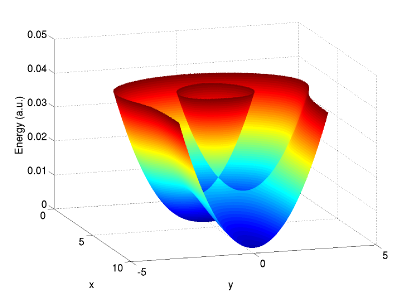
Figure 1: Model potentials in the adiabatic representation.

Transforming the problem to the adiabatic representation gives rise to a CI (Fig. 1). Considering that CI’s energy ($E_{\rm CI}\approx 0.015$) is higher than the energy of the ground state of the $V_{b}$ potential ($0.012$), one can conclude that the Born-Oppenheimer approximation (BOA) may be quite adequate at least for this state. It turns out that switching to the BOA destroys the bound state and gives rise to a resonance state. This shows that purely energetic consideration is not accurate in this case and some symmetry is broken when the BOA is introduced.

Generally, conical intersections (CIs) not only promote transitions between different electronic states but also introduce Berry or geometric phase (GP).Longuet-Higgins et al. (1958); Berry (1984); Ryabinkin, Joubert-Doriol, and Izmaylov (2017) The manifestation of GP is in changing a sign of the electronic wavefunction upon a continuous evolution along a closed path encircling a CI. To ensure that the total wavefunction is single-valued, the nuclear wavefunction must also change the sign. This sign change can be introduced via a phase factor that is position-dependent and constitutes exponential function of the GP. GP is a feature of the adiabatic representation and does not appear in the diabatic representation. In several instances GP played a crucial role in obtaining qualitatively correct results when problems were considered in the adiabatic representationRyabinkin and Izmaylov (2013); Kendrick (1997); Ham (1987); Xie et al. (2016, 2017); Xie and Guo (2017); Xie, Yarkony, and Guo (2017). Therefore, it is quite natural to inquire whether the GP is the reason for appearance of BSCs in this system.

Methods: To investigate the role of the GP we will consider time-independent Schrödinger equation for four Hamiltonians. The original diabatic Hamiltonian $H_{\rm dia}$ [Eq. (1)] is used as a reference that includes all contributions: nonadiabatic transitions and GP effects. In contrast, the Born-Oppenheimer (BO) Hamiltonian $H_{\rm BO}$ does not have any of these effects. Formally, to obtain $H_{\rm BO}$ one needs to diagonalize the potential matrix in $H_{\rm dia}$ using the unitary matrix

$$U=\begin{pmatrix}\cos\theta&\sin\theta\\ -\sin\theta&\cos\theta\end{pmatrix}$$ (4)

where angle $\theta$ is

$$\theta(x,y)=\frac{1}{2}\arctan\dfrac{2\,V_{bc}}{V_{c}-V_{b}}.$$ (5)

Removing the high energy electronic state and nonadiabatic couplings gives

$$H_{\rm BO}=T_{N}+W_{-},$$ (6)

where

$$W_{-}=\frac{1}{2}\left(V_{b}+V_{c}\right)-\frac{1}{2}\sqrt{\left(V_{b}-V_{c}\right)^{2}+4V_{bc}^{2}}.$$ (7)

To include GP in the BO representation we use the Mead and Truhlar approachMead and Truhlar (1979), where the double-valued projector $e^{-i\theta}$ is applied to $H_{\rm BO}$ to avoid working with double-valued nuclear wavefunctions. This results in our third Hamiltonian

$$H^{\rm GP}_{\rm BO} = e^{i\theta}H_{\rm BO}e^{-i\theta}$$ (8)

$$= T_{N}+\tau_{\rm GP}+W_{-},$$

where

$$\tau_{\rm GP}=\frac{\left(\nabla\theta\right)^{2}}{2}+i\nabla\theta\nabla+\frac{i}{2}\nabla^{2}\theta,$$ (9)

and $\nabla=(\sqrt{\omega_{x}}\partial_{x},\sqrt{\omega_{y}}\partial_{y})$. $H^{\rm GP}_{\rm BO}$ includes only the GP effects but excludes all nonadiabatic transitions.

Finally, to obtain a picture where nonadiabatic transitions are preserved but GP effects are removed, we use the diabatic Hamiltonian identical to $H_{\rm dia}$ but with modified $V_{bc}=c|y|$. Introducing the absolute value function in the coupling was shown to remove the GP when the diabatic-to-adiabatic transformation is done.Izmaylov, Li, and Joubert-Doriol (2016) We will refer to this Hamiltonian as $H_{\rm dia}^{\rm noGP}$. An alternative to $H_{\rm dia}^{\rm noGP}$ can be a Hamiltonian obtained by transforming $H_{\rm dia}$ to the adiabatic representation and ignoring the double-valued boundary conditions introduced by this transformation. The main advantage of $H_{\rm dia}^{\rm noGP}$ is numerical robustness of the diabatic representation.

To determine if an eigenstate is a bound or resonant state, its lifetime is calculated using the stabilization method.Mandelshtam, Ravuri, and Taylor (1993) Stabilization graphs are used to obtain complex energies in the form $E=E_{R}-i\Gamma/2$, where $E_{R}$ is the real part and $\Gamma$ is inversely proportional to the lifetime of the state.Moiseyev (2011) A finite lifetime of the state is an indication of its resonance character.

Figure 2: Stabilization graphs for the lowest localized state of various Hamiltonians: a) $H_{\rm dia}$, b) $H_{\rm BO}$, c) $H_{\rm BO}^{\rm GP}$, and d) $H_{\rm dia}^{\rm noGP}$.

All Hamiltonians are transformed to matrices using static basis functions. The same product basis of functions in $x$ and $y$ directions was used for the two electronic states of the diabatic Hamiltonians as well as for the single electronic state adiabatic Hamiltonians. Particle in a box (PB) eigenfunctions were used in the $x$-direction. These functions introduce the length of the box as a natural stabilization parameter for the stabilization method.Mandelshtam, Ravuri, and Taylor (1993) The box interval $[-4,L]$ chosen to cover both bound and continuum parts of the potential (Eqs. (2) and (3)). Harmonic oscillator eigenfunctions were used in the $y$-direction. Energy of low lying states for all Hamiltonians converged within $10^{-6}$ a.u. with 150 PB and 20 harmonic oscillator eigenfunctions.

Results: Table 1 and Figs. 2 and 3 summarize results of stabilization calculations for the lowest localized states of the four Hamiltonians. The Hamiltonians accounting for GP effects have only real components of energy up to a numerical error, while removing GP effects leads to a resonance character of the lowest localized state. Thus, the BSC can be clearly related to the presence of the GP. An intuitive picture of this relation is that in the absence of the GP the nuclear wave-packet can tunnel through a barrier separating the bound part of the $W_{-}$ potential from its unbound counterpart, whereas addition of the GP creates destructive interference between the parts of the wave-packet that tunnel through the barrier on different sides of the CI.

Table 1: The energies of the lowest localized state of different Hamiltonians (in $10^{-3}$ a.u.).

$H_{\rm dia}$	$H_{\rm BO}$	$H_{\rm BO}^{\rm GP}$	$H_{\rm dia}^{\rm noGP}$
$10.29$	$9.23-i0.10$	$10.23$	$10.02-i0.04$

The absolute overlap of the $H_{\rm dia}$ and $H_{\rm BO}^{\rm GP}$ wavefunctions, $|\langle\Psi_{\rm dia}|\Psi_{\rm BO}^{\rm GP}\rangle|$ is 0.93, which is relatively large considering that the total probability to find the system described by $|\Psi_{\rm dia}\rangle$ in the ground electronic electronic state is 0.97 (see also Fig. 3 (a) and (c)).

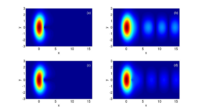
Figure 3: Contour of the square root of the ground electronic state nuclear probability density of the lowest localized state for different Hamiltonians with box length $20.4$ a.u.: a) $H_{\rm dia}$, b) $H_{\rm BO}$, c) $H_{\rm BO}^{\rm GP}$, and d) $H_{\rm dia}^{\rm noGP}$.

In conclusion, we have unambiguously shown that the nontrivial GP is the reason for bound states in the continuum in the considered model problem. This result is yet another illustration that inclusion of the GP can qualitatively change results in nonadiabatic problems and cannot be ignored a priori. The current result is a direct analog of GP induced localization obtained in the double-well potential problemRyabinkin and Izmaylov (2013); Joubert-Doriol and Izmaylov (2017). As in the double-well case, one can expect that there is a certain range of parameters of the linear vibronic model that supports the BSC. This is in accord with previous works on GP effects in tunneling that did not find BSCs for a very similar model with different values of corresponding parametersXie and Guo (2017); Xie, Yarkony, and Guo (2017). Yet, one can hope that it is possible to engineer a molecular system where GP will not only slow down the tunneling process but will completely freeze it by giving rise to BSCs.

Acknowledgements: The authors thank Ilya Ryabinkin and Loïc Joubert-Doriol for helpful discussions. This work was supported by a Sloan Research Fellowship, Natural Sciences and Engineering Research Council of Canada (NSERC), and an Ontario Graduate Scholarship (OGS).

References

- von Neumann and Wigner (1929) J. von Neumann and E. Wigner, Phys. Z. 30, 465 (1929).
- Capasso et al. (1992) F. Capasso, C. Sirtori, J. Faist, D. L. Sivco, S.-N. G. Chu, and A. Y. Cho, Nature 358, 565 (1992).
- Hsu et al. (2013) C. W. Hsu, B. Zhen, J. Lee, S.-L. Chua, S. G. Johnson, J. D. Joannopoulos, and M. Soljacic, Nature 499, 188 (2013).
- Kodigala et al. (2017) A. Kodigala, T. Lepetit, Q. Gu, B. Bahari, Y. Fainman, and B. Kanté, Nature 541, 196 (2017).
- Moiseyev (2009) N. Moiseyev, Phys. Rev. Lett. 102, 167404 (2009).
- Sadrieva et al. (2017) Z. F. Sadrieva, I. S. Sinev, K. L. Koshelev, A. Samusev, I. V. Iorsh, O. Takayama, R. Malureanu, A. A. Bogdanov, and A. V. Lavrinenko, ACS Photonics 4, 723 (2017).
- Hsu et al. (2016) C. W. Hsu, B. Zhen, A. D. Stone, J. D. Joannopoulos, and M. Soljac̆ić, Nat. Rev. Mater. 1, 16048 (2016).
- Cederbaum et al. (2003) L. Cederbaum, R. Friedman, V. Ryaboy, and N. Moiseyev, Phys. Rev. Lett. 90, 013001 (2003).
- Longuet-Higgins et al. (1958) H. C. Longuet-Higgins, U. Opik, M. H. L. Pryce, and R. A. Sack, Proc. R. Soc. A 244, 1 (1958).
- Berry (1984) M. V. Berry, Proc. R. Soc. A 392, 45 (1984).
- Ryabinkin, Joubert-Doriol, and Izmaylov (2017) I. G. Ryabinkin, L. Joubert-Doriol, and A. F. Izmaylov, Acc. Chem. Res. 50, 1785 (2017).
- Ryabinkin and Izmaylov (2013) I. G. Ryabinkin and A. F. Izmaylov, Phys. Rev. Lett. 111, 220406 (2013).
- Kendrick (1997) B. Kendrick, Phys. Rev. Lett. 79, 2431 (1997).
- Ham (1987) F. S. Ham, Phys. Rev. Lett. 58, 725 (1987).
- Xie et al. (2016) C. Xie, J. Ma, X. Zhu, D. R. Yarkony, D. Xie, and H. Guo, J. Am. Chem. Soc. 138, 7828 (2016).
- Xie et al. (2017) C. Xie, B. K. Kendrick, D. R. Yarkony, and H. Guo, J. Chem. Theory Comput. 13, 1902 (2017).
- Xie and Guo (2017) C. Xie and H. Guo, Chem. Phys. Lett. 683, 222 (2017).
- Xie, Yarkony, and Guo (2017) C. Xie, D. R. Yarkony, and H. Guo, Phys. Rev. A 95, 022104 (2017).
- Mead and Truhlar (1979) C. A. Mead and D. G. Truhlar, J. Chem. Phys. 70, 2284 (1979).
- Izmaylov, Li, and Joubert-Doriol (2016) A. F. Izmaylov, J. Li, and L. Joubert-Doriol, J. Chem. Theory Comput. 12, 5278 (2016).
- Mandelshtam, Ravuri, and Taylor (1993) V. A. Mandelshtam, T. R. Ravuri, and H. S. Taylor, Phys. Rev. Lett. 70, 1932 (1993).
- Moiseyev (2011) N. Moiseyev, Non-Hermitian Quantum Mechanics (Cambridge University Press, Cambridge, 2011).
- Joubert-Doriol and Izmaylov (2017) L. Joubert-Doriol and A. F. Izmaylov, Chem. Commun. 53, 7365 (2017).