Overview of the Incompressible Navier–Stokes simulation capabilities in the MOOSE Framework

Abstract

The Multiphysics Object Oriented Simulation Environment (MOOSE) framework is a high-performance, open source, C⁺⁺ finite element toolkit developed at Idaho National Laboratory. MOOSE was created with the aim of assisting domain scientists and engineers in creating customizable, high-quality tools for multiphysics simulations. While the core MOOSE framework itself does not contain code for simulating any particular physical application, it is distributed with a number of physics “modules” which are tailored to solving e.g. heat conduction, phase field, and solid/fluid mechanics problems. In this report, we describe the basic equations, finite element formulations, software implementation, and regression/verification tests currently available in MOOSE’s navier_stokes module for solving the Incompressible Navier–Stokes (INS) equations.

1 Introduction

The MOOSE framework [1], which has been under development since 2008 and LGPL-2.1 licensed open source software on GitHub since March 2014 [2], was originally created to facilitate the development of sophisticated simulation tools by domain experts in fields related to nuclear power generation (neutron transport, nuclear fuel performance, mesoscale material modeling, thermal hydraulics, etc.) who were not necessarily experts in computational science. A guiding principle in the development of the MOOSE framework is: by lowering the typical computational science-related barriers of entry, e.g. knowledge of low-level programming languages, familiarity with parallel programming paradigms, and complexity/lack of interfaces to existing numerical software libraries, one can substantially increase the number and quality of scientific contributions to the aforementioned fields in a cost-effective, sustainable, and scientifically sound manner.

The generality and applicability of MOOSE stems directly from that of the finite element method (FEM) itself. MOOSE relies on the libMesh [3] library’s mesh handling, geometric/finite element families, and numerical linear algebra library [4] interfaces to avoid code duplication, and focuses on providing a consistent set of interfaces which allow users to develop custom source code and input file syntax into application-specific simulation tools. In the research and development environment, one frequently simulates physics involving the combination of a well-established mathematical model (heat conduction, solid mechanics, etc.) alongside a new or as-yet-untested collection of models. The MOOSE physics modules were created to help ensure that these types of combinations were not only possible, but also relatively painless to create.

There are currently in the neighborhood of a dozen actively developed MOOSE physics modules. The heat_conduction module, for example, can be used to solve the transient solid heat conduction equation,

$$\rho c_{p}\frac{\partial T}{\partial t} =\nabla\cdot k\nabla T+f$$ (1)

where $\rho$, $c_{p}$, and $k$ are the density, specific heat, and thermal conductivity, respectively, of the medium, $T$ is the unknown temperature, and $f$ is a volumetric heat source term. This module supports both single- and multi-domain solves using Lagrange multiplier and gap heat transfer finite element formulations. The tensor_mechanics module focuses on solving linear elastic and finite strain solid mechanics equations of the form

$$\nabla\cdot\left(\bm{\sigma}+\bm{\sigma}_{0}\right)+\vec{b}=\vec{0}$$ (2)

where $\bm{\sigma}$ is the Cauchy stress tensor, $\bm{\sigma}_{0}$ is an “extra” stress due to e.g. coupling with other physics, and $\vec{b}$ is a possibly temperature-dependent body force which can be used to couple together the tensor_mechanics and heat_conduction modules. Likewise, the phase_field module can be used to solve the Allen–Cahn [5] and Cahn–Hilliard [6, 7] equations:

$$\frac{\partial\eta_{j}}{\partial t} =-L_{j}\frac{\delta F}{\delta\eta_{j}}$$ (3)

$$\frac{\partial c_{i}}{\partial t} =\nabla\cdot\left(M_{i}\nabla\frac{\delta F}{\delta c_{i}}\right)$$ (4)

for the non-conserved ($\eta_{j}$) and conserved ($c_{i}$) order parameters, where the free energy functional $F$ can depend on both the temperature $T$ and stress field $\bm{\sigma}$ computed by the heat_conduction and tensor_mechanics modules, respectively.

MOOSE’s navier_stokes module, which is the subject of the present work, is capable of solving both the compressible and incompressible Navier–Stokes equations using a variety of Petrov–Galerkin, discontinuous Galerkin (DG), and finite volume (implemented as low-order DG) discretizations. Here, we focus only on the incompressible version of the Navier–Stokes equations, since the numerical techniques used for the compressible version are significantly different and will be discussed in a future publication. One of the more compelling reasons for developing an INS solver capability as a MOOSE module is the potential for coupling it to the MOOSE modules just listed, as well as others: fluid-structure interaction problems could eventually be tackled via coupling to the tensor_mechanics module, immiscible fluid interface topology tracking with realistic divergence-free flow fields could be implemented via coupling to the level_set module, and chemically-reacting flows could be investigated by coupling to the chemical_reactions module.

The INS equations are an important tool for investigating many types of physical applications where viscous effects cannot readily be neglected, including aerodynamic drag calculations, turbulence modeling, industrial lubrication, boundary layers, and pipe flows, to name just a few. A number of classic textbooks [8, 9, 10, 11] have been written on the historical development and present-day understanding of incompressible flow models. The widespread use of the FEM for simulating incompressible flow problems postdates its use as the tool of choice for structural analysis problems, but relatively recent theoretical, numerical, and computational advances from the 1980s to the present day have led to a dramatic increase in its popularity. The numerical methods employed in the navier_stokes module generally follow well-established trends in the field at large and are based largely on the many reference texts [12, 13, 14, 15, 16, 17] available in this area. The intent of this article is therefore not to describe new developments in the field of finite element modeling for incompressible fluids, but rather to elucidate an open, extensible, community-developed approach for applying established and proven techniques.

The rest of this paper is arranged as follows: in §2 the relevant forms of the governing equations are briefly described, and in §3 details of the numerical method employed in the navier_stokes module are discussed, including weak formulations, stabilized FEM, time discretizations, and solvers. In §4 we describe in more detail the overarching design of the MOOSE framework itself and the implications of that design in the development of the navier_stokes module. In §5, several of the verification tests which form the backbone of our regression testing and continuous integration based software development process are characterized, and finally, in §6 we discuss some representative applications which demonstrate the effectiveness and usefulness of the software.

2 Governing equations

The navier_stokes module in MOOSE can be used to solve the INS equations of fluid flow in 2D and 3D Cartesian coordinates as well as 2D-axisymmetric (referred to as “RZ” in the code) coordinates. Two variants of the governing equations, the so-called “traction” and “Laplace” forms, are supported. The two forms differ primarily in the constant viscosity assumption, and the resulting form of the natural boundary conditions [18]. Detailed descriptions are provided in §2.1 and §2.2, respectively.

2.1 Traction form

The “traction” form of the INS equations, so-called because the natural boundary condition involves the surface traction vector, can be expressed in the following compact form:

$$\vec{R}(\vec{U})=\vec{0}$$ (5)

where $\vec{U}\equiv(\vec{u},p)$ is a vector composed of the velocity and pressure unknowns, and

$$\vec{R}(\vec{U})\equiv\begin{bmatrix}\rho\left(\displaystyle\frac{\partial\vec{u}}{\partial t}+(\vec{u}\cdot\text{grad}\,\!)\vec{u}\right)-\text{div}\,\bm{\sigma}-\vec{f}\\[12.0pt] \text{div}\,\vec{u}\end{bmatrix}$$ (6)

where $\rho$ is the (constant) fluid density, $\vec{f}$ is a body force per unit volume, and $\bm{\sigma}$ is the total stress tensor, defined by:

$$\bm{\sigma} \equiv-p\bm{I}+\bm{\tau}$$

$$=-p\bm{I}+\mu\left(\text{grad}\,\vec{u}+(\text{grad}\,\vec{u})^{T}\right)$$ (7)

In (7), $\mu$ is the dynamic viscosity, $\bm{I}$ is the identity matrix, and $\bm{\tau}$ is the viscous stress tensor. In the present work, we consider only Newtonian fluids, but the extension of our formulation to other types of fluids is straightforward. In (7), we have a priori neglected the dilatational viscosity contribution, $\lambda\left(\text{div}\,\vec{u}\right)\bm{I}$, where the second coefficient of viscosity $\lambda=-\frac{2\mu}{3}$ [19]. This term is dropped based on the divergence-free constraint (second row of (6)), but it could be retained, and in fact it is connected to a particular form of numerical stabilization that will be discussed in §3.2.3. Finally, we note that while variants of the convective operator in (6), including $\text{curl}\,\vec{u}\times\vec{u}+\frac{1}{2}\text{grad}\,|\vec{u}|^{2}$ (rotation form) and $\frac{1}{2}\left((\vec{u}\cdot\text{grad}\,\!)\vec{u}+\text{div}\,\vec{u}\vec{u}\right)$ (skew-symmetric form), can be useful under certain circumstances [20], only the form shown in (6) is implemented in the navier_stokes module.

2.2 Laplace form

As mentioned previously, the density $\rho$ of an incompressible fluid is, by definition, a constant, and therefore can be scaled out of the governing equations without loss of generality. In the navier_stokes module, however, $\rho$ is maintained as an independent, user-defined constant and the governing equations are solved in dimensional form. Although there are many benefits to using non-dimensional formulations, it is frequently more convenient in practice to couple with other simulation codes using a dimensional formulation, and this motivates the present approach.

The remaining material property, the dynamic viscosity $\mu$, is also generally constant for isothermal, incompressible fluids, but may depend on temperature, especially in the case of gases. In the navier_stokes module, we generally allow $\mu$ to be non-constant in (7), but if $\mu$ is constant, we can make the following simplification:

$$\text{div}\,\bm{\sigma} =\text{div}\,\left(-p\bm{I}+\mu\left(\text{grad}\,\vec{u}+(\text{grad}\,\vec{u})^{T}\right)\right)$$

$$=-\text{grad}\,p+\mu\left(\text{div}\,\text{grad}\,\vec{u}+\text{div}\,(\text{grad}\,\vec{u})^{T}\right)$$

$$=-\text{grad}\,p+\mu\left(\text{grad}\,(\text{div}\,\vec{u})+\text{div}\,(\text{grad}\,\vec{u})^{T}\right)$$

$$=-\text{grad}\,p+\mu\,\text{div}\,(\text{grad}\,\vec{u})^{T}$$

$$=-\text{grad}\,p+\mu\,\text{Lap}\,\vec{u}$$ (8)

where $\text{Lap}\,\vec{u}\equiv\text{div}\,(\text{grad}\,\vec{u})^{T}$ is the vector Laplacian operator (which differs from component-wise application of the scalar Laplacian operator in e.g. cylindrical coordinates). Note that in the derivation of (8) we also assumed sufficient smoothness in $\vec{u}$ to interchange the order of differentiation in the third line, and we used the incompressibility constraint to drop the first term in parentheses on line 4. The “Laplace” form of (5) is therefore given by:

$$\vec{R}_{L}(\vec{U})=\vec{0}$$ (9)

where

$$\vec{R}_{L}(\vec{U})\equiv\begin{bmatrix}\rho\left(\displaystyle\frac{\partial\vec{u}}{\partial t}+(\vec{u}\cdot\text{grad}\,\!)\vec{u}\right)+\text{grad}\,p-\mu\,\text{Lap}\,\vec{u}-\vec{f}\\[12.0pt] \text{div}\,\vec{u}\end{bmatrix}$$ (10)

In the continuous setting, Eqn. (9) is equivalent to (5) provided that the constant viscosity assumption is satisfied. In the discrete setting, when the velocity field is not necessarily pointwise divergence-free, the approximate solutions resulting from finite element formulations of the two equation sets will not necessarily be the same. In practice, we have observed significant differences in the two formulations near outflow boundaries where the natural boundary condition is weakly imposed. The navier_stokes module therefore implements both (5) and (9), and the practitioner must determine which is appropriate in their particular application.

Equations (5) and (9) are valid in all of the coordinate systems mentioned at the beginning of this section, provided that the proper definitions of the differential operators “grad” and “div” are employed. The governing equations are solved in the spatiotemporal domain $(\vec{x},t)\in\Omega\times(0,T)$ where $\Omega$ has boundary $\Gamma$ and outward unit normal $\hat{n}$, and the full specification of the problem is of course incomplete without the addition of suitable initial and boundary conditions. In the navier_stokes module, we support the usual Dirichlet ($\vec{u}=\vec{g}\in\Gamma_{D}\subset\Gamma$) and surface traction ($\hat{n}\cdot\bm{\sigma}=\vec{s}\in\Gamma_{N}\subset\Gamma$) boundary conditions, as well as several others that are applicable in certain specialized situations. Initial conditions on the velocity field, which must satisfy the divergence-free constraint, are also required, and may be specified as constants, data, or in functional form.

3 Numerical method

The navier_stokes module solves the traction (5) and Laplace (9) form of the INS equations, plus initial and boundary conditions, using a stabilized Petrov–Galerkin FEM. The development of this FEM follows the standard recipe: first, weak formulations are developed for prototypical boundary conditions in §3.1, then the semi-discrete stabilized finite element formulation is introduced in §3.2, followed by the time discretization in §3.3. Finally, in §3.4 some details on the different types of preconditioners and iterative solvers available in the navier_stokes module are provided.

3.1 Weak formulation

To develop a weak formulation for (5), we consider the combined Dirichlet/flux boundary and initial conditions

$$\vec{u} =\vec{g} \;\in\Gamma_{D}$$ (11)

$$\hat{n}\cdot\bm{\sigma} =\vec{s} \;\in\Gamma_{N}$$ (12)

$$\vec{u} =\vec{u}_{0} \;\in\Omega\text{ at }t=0$$ (13)

where $\vec{g}$ and $\vec{s}$ are given (smooth) boundary data, and $\Gamma=\Gamma_{D}\cup\Gamma_{N}$ is the entire boundary of $\Omega$. The weak formulation of (5) with conditions (11)–(13) is then: find $\vec{U}\in\mathcal{S}$ such that

$$a(\vec{U},\vec{V})=0$$ (14)

holds for every $\vec{V}\in\mathcal{V}$, where

$$a(\vec{U},\vec{V}) \equiv\int_{\Omega}\left[\rho\left(\frac{\partial\vec{u}}{\partial t}+(\vec{u}\cdot\text{grad}\,\!)\vec{u}\right)\cdot\vec{v}-p\,\text{div}\,\vec{v}+\bm{\tau}:\text{grad}\,\vec{v}-\vec{f}\cdot\vec{v}\right]\text{d}\Omega$$

$$\qquad-\int_{\Gamma_{N}}\vec{s}\cdot\vec{v}\;\text{d}\Gamma-\int_{\Omega}q\,\text{div}\,\vec{u}\;\text{d}\Omega$$ (15)

and the relevant function spaces are

$$\mathcal{S} =\{\vec{U}=(\vec{u},p):u_{i},p\in H^{1}(\Omega)\times C^{0}(0,T),\,\vec{u}=\vec{g}\in\Gamma_{D}\}$$ (16)

$$\mathcal{V} =\{\vec{V}=(\vec{v},q):v_{i},q\in H^{1}(\Omega)\times C^{0}(0,T),\,\vec{v}=\vec{0}\in\Gamma_{D}\}$$ (17)

where $\Omega\subset\mathbb{R}^{n_{s}}$, $n_{s}$ is the spatial dimension of the problem, $H^{1}(\Omega)$ is the Hilbert space of functions with square-integrable generalized first derivatives defined on $\Omega$, and the colon operator denotes tensor contraction, i.e. $\bm{A}\colon\!\!\bm{B}\equiv A_{ij}B_{ij}$. We remark that this weak formulation can be derived by dotting (5) with a test function $\vec{V}\equiv(\vec{v},q)$, integrating over $\Omega$, and applying the following identity/divergence theorem:

$$\int_{\Omega}\vec{v}\cdot\text{div}\,\bm{S}\;\text{d}{\Omega} =\int_{\Omega}\text{div}\,(\bm{S}\vec{v})\;\text{d}{\Omega}-\int_{\Omega}\bm{S}^{T}\colon\text{grad}\,\vec{v}\;\text{d}{\Omega}$$

$$=\int_{\Gamma}(\bm{S}\vec{v})\cdot\hat{n}\;\text{d}{\Gamma}-\int_{\Omega}\bm{S}^{T}\colon\text{grad}\,\vec{v}\;\text{d}{\Omega}$$

$$=\int_{\Gamma}(\hat{n}\cdot\bm{S})\cdot\vec{v}\;\text{d}{\Gamma}-\int_{\Omega}\bm{S}^{T}\colon\text{grad}\,\vec{v}\;\text{d}{\Omega}$$ (18)

which holds for the general (not necessarily symmetric) tensor $\bm{S}$. In the development of the FEM, we will extract the individual component equations of (15) by considering linearly independent test functions $\vec{V}=(v\hat{e}_{i},0)$, $i=1,\ldots,n_{s}$, where $\hat{e}_{i}$ is a unit vector in $\mathbb{R}^{n_{s}}$, and $\vec{V}=(\vec{0},q)$.

For the “Laplace” version (9) of the governing equations, we consider the same Dirichlet and initial conditions as before, and a slightly modified version of the flux condition (12) given by

$$\hat{n}\cdot\left(\mu\left(\text{grad}\,\vec{u}\right)^{T}-p\bm{I}\right) =\vec{s}\;\in\Gamma_{N}$$ (19)

The weak formulation for the Laplace form of the governing equations is then: find $\vec{U}\in\mathcal{S}$ such that

$$a_{L}(\vec{U},\vec{V})=0$$ (20)

holds for every $\vec{V}\in\mathcal{V}$, where

$$a_{L}(\vec{U},\vec{V}) \equiv\int_{\Omega}\left[\rho\left(\frac{\partial\vec{u}}{\partial t}+(\vec{u}\cdot\text{grad}\,\!)\vec{u}\right)\cdot\vec{v}-p\,\text{div}\,\vec{v}+\mu\left(\text{grad}\,\vec{u}:\text{grad}\,\vec{v}\right)-\vec{f}\cdot\vec{v}\right]\text{d}\Omega$$

$$\qquad-\int_{\Gamma_{N}}\vec{s}\cdot\vec{v}\;\text{d}\Gamma-\int_{\Omega}q\,\text{div}\,\vec{u}\;\text{d}\Omega$$ (21)

The main differences between (21) and (15) are thus the form of the viscous term in the volume integral (although both terms are symmetric) and the definition of the Neumann data $\vec{s}$. Both (15) and (21) remain valid in any of the standard coordinate systems, given suitable definitions for the “grad,” “div,” and integration operations. As a matter of preference and historical convention, we have chosen the sign of the $q\,\text{div}\,\vec{u}$ term in both (15) and (21) to be negative. This choice makes no difference in the weak solutions $(\vec{u},p)$ which satisfy (15) and (21), but in the special case of Stokes’ flow (in which the convective term $(\vec{u}\cdot\text{grad}\,\!)\vec{u}$ can be neglected), it ensures that the stiffness matrices resulting from these weak formulations are symmetric.

3.1.1 Boundary conditions

A few notes on boundary conditions are also in order. In the case of a pure Dirichlet problem, i.e. when $\Gamma_{D}=\Gamma$ and $\Gamma_{N}=\emptyset$, the pressure $p$ in both the strong and weak formulations is only determined up to an arbitrary constant. This indeterminacy can be handled in a variety of different ways, for instance by requiring that a global “mean-zero pressure” constraint [21], $\int_{\Omega}p\;\text{d}\Omega=0$, hold in addition to the momentum balance and mass conservation equations discussed already, or by using specialized preconditioned Krylov solvers [22, 23] for which the non-trivial nullspace of the operator can be pre-specified. A more practical/simplistic approach is to specify a single value of the pressure at some point in the domain, typically on the boundary. This approach, which we generally refer to as “pinning” the pressure, is frequently employed in the navier_stokes module to avoid the difficulties associated with the non-trivial nullspace of the operator.

In both (15) and (21), we have applied the divergence theorem to (integrated by parts) the pressure term as well as the viscous term. While this is the standard approach for weak formulations of the INS equations, it is not strictly necessary to integrate the pressure term by parts. Not integrating the pressure term by parts, however, both breaks the symmetry of the Stokes problem discussed previously, and changes the form and meaning of the Neumann boundary conditions (12) and (19). In particular, the “combined” boundary condition formulation of the problem is no longer sufficient to constrain away the nullspace of constant pressure fields, and one must instead resort to either pressure pinning or one of the other approaches discussed previously. Nevertheless, there are certain situations where the natural boundary condition imposed by not integrating the pressure term by parts is useful in simulation contexts, and therefore the navier_stokes module provides the user-selectable boolean flag integrate_p_by_parts to control this behavior.

It is common for applications with an “outflow” boundary to employ the so-called “natural” boundary condition, which corresponds to setting $\vec{s}=\vec{0}$, where $\vec{s}$ is defined in (12) and (19) for the traction and Laplace forms, respectively. A drawback to imposing the natural boundary condition is that, unless the flow is fully developed, this condition will influence the upstream behavior of the solution in a non-physical way. In order to avoid/alleviate this issue, one can artificially extend the computational domain until the flow either becomes fully developed or the upstream influence of the outlet boundary is judged to be acceptably small.

Another alternative is to employ the so-called “no-BC” boundary condition described by Griffiths [24]. In the no-BC boundary condition, the residual contribution associated with the boundary term is simply computed and accumulated along with the other terms in the weak form. The no-BC boundary condition is therefore distinct from the natural boundary condition, and can be thought of as not specifying any “data” at the outlet, which is not strictly valid for uniformly elliptic partial differential equations (PDE). Nevertheless, Griffiths showed, for the 1D scalar advection-diffusion equation discretized with finite elements, that the no-BC boundary condition appears to influence the upstream behavior of the solution less than the natural boundary condition. The navier_stokes module includes both traction and Laplace forms of the no-BC boundary condition via the INSMomentumNoBCBCTractionForm and INSMomentumNoBCBCLaplaceForm classes, respectively.

3.2 Stabilized finite element method

To construct the FEM, we discretize $\Omega$ into a non-overlapping set of elements $\mathcal{T}^{h}$ and introduce the approximation spaces $\mathcal{S}^{h}\subset\mathcal{S}$ and $\mathcal{V}^{h}\subset\mathcal{V}$, where

$$\mathcal{S}^{h} =\{\vec{U}_{h}=(\vec{u}_{h},p_{h}):{u}^{h}_{i}\in\mathcal{G}^{k},p_{h}\in\mathcal{G}^{r},\,\vec{u}_{h}=\vec{g}\in\Gamma_{D}\}$$ (22)

$$\mathcal{V}^{h} =\{\vec{V}_{h}=(\vec{v}_{h},q_{h}):{v}^{h}_{i}\in\mathcal{G}^{k},q_{h}\in\mathcal{G}^{r},\,\vec{v}_{h}=\vec{0}\in\Gamma_{D}\}$$ (23)

and

$$\mathcal{G}^{k}\equiv\{w\in C^{0}(\Omega)\times C^{0}(0,T),\,\left.w\right|_{\Omega_{e}}\in\mathcal{P}^{k}(\Omega_{e}),\;\forall\,\Omega_{e}\in\mathcal{T}^{h}\}$$ (24)

where ${u}^{h}_{i}$ is the $i$th component of $\vec{u}_{h}$, and $\mathcal{P}^{k}(\Omega_{e})$ is either the space of complete polynomials of degree $k$ (on triangular and tetrahedral elements) or the space of tensor products of polynomials of degree $k$ (on quadrilateral and hexahedral elements) restricted to element $\Omega_{e}$. For brevity we shall subsequently follow the standard practice and refer to discretizations of the former type as “$P^{k}P^{r}$ elements” and the latter as “$Q^{k}Q^{r}$ elements.” Although it is generally possible to employ non-conforming velocity elements and constant or discontinuous ($\subset L^{2}(\Omega)$) pressure elements [25], we have not yet implemented such discretizations in the navier_stokes module, and do not describe them in detail here.

The spatially-discretized (continuous in time) version of the weak formulation (14) is thus: find $\vec{U}_{h}\in\mathcal{S}^{h}$ such that

$$a(\vec{U}_{h},\vec{V}_{h})=0$$ (25)

holds for every $\vec{V}_{h}\in\mathcal{V}^{h}$. The semi-discrete weak formulation for the Laplace form (20) is analogous. Not all combinations of polynomial degrees $k$ and $r$ generate viable (i.e. Ladyzhenskaya–Babuška–Brezzi (LBB) stable [26, 27, 28]) mixed finite element formulations. A general rule of thumb is that the velocity variable’s polynomial degree must be at least one order higher than that of the pressure, i.e. $k\geq r+1$; however, we will discuss equal-order discretizations in more detail momentarily.

In addition to instabilities arising due to incompatibilities between the velocity and pressure approximation spaces, numerical approximations of the INS equations can also exhibit instabilities in the so-called advection-dominated regime. The INS equations are said to be advection-dominated (in the continuous setting) when $\text{Re}\gg 1$, where $\text{Re}\equiv\frac{\rho|\vec{u}|L}{\mu}$ is the Reynolds number based on a characteristic length scale $L$ of the application. Galerkin finite element approximations such as (25) are known to produce highly-oscillatory solutions in the advection-dominated limit, and are therefore of severely limited utility in many real-world applications. To combat each of these types of instabilities, we introduce the following stabilized weak statement associated with (25): find $\vec{U}_{h}\in\mathcal{S}^{h}$ such that

$$a(\vec{U}_{h},\vec{V}_{h})+\int_{\Omega^{\prime}}\vec{S}(\vec{U}_{h},\vec{V}_{h})\cdot\vec{R}(\vec{U}_{h})\;\text{d}\Omega^{\prime}=0$$ (26)

holds for every $\vec{V}_{h}\in\mathcal{V}^{h}$, where

$$\vec{S}(\vec{U}_{h},\vec{V}_{h})\equiv\begin{bmatrix}\tau_{\text{SUPG}}\,(\vec{u}_{h}\cdot\text{grad}\,\!)\vec{v}_{h}+\rho^{-1}\,\tau_{\text{PSPG}}\,\text{grad}\,q_{h}\\[12.0pt] \rho\,\tau_{\text{LSIC}}\,(\text{div}\,\vec{v}_{h})\end{bmatrix}$$ (27)

is the stabilization operator, $\Omega^{\prime}$ is the union of element interiors,

$$\int_{\Omega^{\prime}}\;\text{d}\Omega^{\prime}\equiv\sum_{\Omega_{e}\in\mathcal{T}^{h}}\int_{\Omega_{e}}\;\text{d}\Omega_{e}$$ (28)

and $\tau_{\text{SUPG}}$, $\tau_{\text{PSPG}}$, and $\tau_{\text{LSIC}}$ are mesh- and solution-dependent coefficients corresponding to Streamline-Upwind Petrov–Galerkin (SUPG), Pressure-Stabilized Petrov–Galerkin (PSPG), and Least-Squares Incompressiblity Constraint (LSIC) techniques, respectively. The stabilized weak formulation for the Laplace form (9) is analogous: $\vec{S}$ remains unchanged, $a_{L}$ replaces $a$, and $\vec{R}_{L}$ replaces $\vec{R}$.

The development of (26) and (27) has spanned several decades, and is summarized succinctly by Donea [29] and the references therein. An important feature of this approach is that it is “consistent,” which in this context means that, if the true solution $\vec{U}$ is substituted into (26), then the $\vec{R}(\vec{U})$ term vanishes, and we recover (25), the original weak statement of the problem. A great deal of research [30, 31, 32, 33, 34] has been conducted over the years to both generalize and unify the concepts of residual-based stabilization methods such as (26) and (27), and current efforts are focused around so-called Variational Multiscale (VMS) and Subgrid Scale (SGS) methods. The three distinct contributions to the stabilization operator used in the present work are briefly summarized below.

3.2.1 SUPG stabilization

The SUPG term introduces residual-dependent artificial viscosity to stabilize the node-to-node oscillations present in Galerkin discretizations of advection-dominated flow [35, 36, 37, 38, 39, 40, 41]. This type of stabilization can be employed independently of the LBB stability of the chosen velocity and pressure finite element spaces. The coefficient $\tau_{\text{SUPG}}$ must have physical units of time so that the resulting term is dimensionally consistent with the momentum conservation equation to which it is added.

Most definitions of $\tau_{\text{SUPG}}$ stem from analysis of one-dimensional steady advection-diffusion problems. For example, the original form of $\tau_{\text{SUPG}}$ for the 1D linear advection-diffusion equation [35] is given by:

$$\tau_{\text{SUPG,opt}} =\frac{h}{2|\vec{u}|}\left(\coth(\text{Pe})-\frac{1}{\text{Pe}}\right)$$ (29)

where $|\vec{u}|$ is the advective velocity magnitude, $h$ is the element size, $\text{Pe}\equiv\frac{|\vec{u}|h}{2k}$ is the element Peclet number, and $k$ is the diffusion coefficient. For piecewise linear elements, this formulation for $\tau_{\text{SUPG}}$ yields a nodally exact solution. An alternative form of $\tau_{\text{SUPG}}$ which yields fourth-order accuracy for the 1D linear advection-diffusion equation [37] is given by:

$$\tau_{\text{SUPG,mod}}=\left[\left(\frac{2|\vec{u}|}{h}\right)^{2}+9\left(\frac{4k}{h^{2}}\right)^{2}\right]^{-\frac{1}{2}}$$ (30)

Note that neither the nodally exact (29) nor the fourth-order accurate (30) forms of the stabilization parameter are directly applicable to 2D/3D advection-diffusion problems or the INS equations. Nevertheless, Eqn. (30) does motivate the $\tau_{\text{SUPG}}$ implementation used in the navier_stokes module, which is given by

$$\tau_{\text{SUPG}}=\alpha\left[\left(\frac{2}{\Delta t}\right)^{2}+\left(\frac{2|\vec{u}|}{h}\right)^{2}+9\left(\frac{4\nu}{h^{2}}\right)^{2}\right]^{-\frac{1}{2}}$$ (31)

where $\Delta t$ is the discrete timestep size (see §3.3), $\nu=\frac{\mu}{\rho}$ is the kinematic viscosity, and $0\leq\alpha\leq 1$ is a user selectable parameter which, among other things, allows the value of $\tau_{\text{SUPG}}$ to be tuned for higher-order elements [42].

3.2.2 PSPG stabilization

The PSPG method was originally introduced [43, 44, 45, 46, 47] in the context of Stokes flow with the aim of circumventing instabilities arising from the use of LBB-unstable element pairs. The motivation for its introduction stems from the fact that LBB-stable finite element pairs, such as the well-known “Taylor–Hood” ($Q^{2}Q^{1}$) element, are often more expensive or simply less convenient to work with than equal-order discretizations. PSPG stabilization is required for LBB-unstable element pairs regardless of whether the flow is advection-dominated.

In the case of Stokes flow, the stabilization parameter $\tau_{\text{PSPG}}$ is given by:

$$\tau_{\text{PSPG}}=\beta\frac{h^{2}}{4\nu}$$ (32)

where $0\leq\beta\leq 1$ is a user-tunable parameter. Decreasing $\beta$ improves the convergence rate of the pressure error in the $L^{2}(\Omega)$ norm, however, using too small a value for $\beta$ will eventually cause equal-order discretizations to lose stability. When this happens, spurious modes (such as the “checkerboard” mode) pollute the discrete pressure solution and produce higher overall error.

Numerical experiments suggest that an optimal value is $\beta\approx 1/3$. Substituting $\beta=1/3$ into (32) yields an expression for $\tau_{\text{PSPG}}$ equivalent to (31) in the case of steady Stokes flow. Consequently, to generalize PSPG stabilization to problems involving advection, we use the same expression for both $\tau_{\text{SUPG}}$ and $\tau_{\text{PSPG}}$, namely (31), in the navier_stokes module. The coefficient $\tau_{\text{PSPG}}$ therefore also has physical units of time, and the $\rho^{-1}$ factor in (27) ensures that the resulting term is dimensionally consistent with the mass conservation equation to which it is added.

3.2.3 LSIC stabilization

The LSIC stabilization term [48, 49, 25, 50] arises naturally in Galerkin Least-Squares (GLS) formulations of the INS equations, and a number of authors have reported that its use leads to improved accuracy and conditioning of the linear systems associated with both LBB-stable and equal-order discretizations. As mentioned when the viscous stress tensor was first introduced in (7), a contribution of the form $-\frac{2\mu}{3}\left(\text{div}\,\vec{u}\right)\bm{I}$ was neglected. Had we retained this term, the weak formulation (15) would have had an additional term of the form

$$\int_{\Omega}-\frac{2\mu}{3}\left(\text{div}\,\vec{u}\right)\left(\text{div}\,\vec{v}\right)\text{d}\Omega$$ (33)

Note the sign of this term, which is the same as that of the pressure term. On the other hand, the $\tau_{\text{LSIC}}$ term implied by (26) is

$$\int_{\Omega^{\prime}}\rho\,\tau_{\text{LSIC}}\left(\text{div}\,\vec{u}_{h}\right)\left(\text{div}\,\vec{v}_{h}\right)\text{d}\Omega^{\prime}$$ (34)

Therefore, we can think of neglecting the $-\frac{2\mu}{3}\left(\text{div}\,\vec{u}\right)\bm{I}$ contribution as effectively introducing a least-squares incompressibility stabilization contribution “for free” with $\tau_{\text{LSIC}}=\frac{2\nu}{3}$.

Implementing the general LSIC stabilization term gives one the flexibility of choosing $\tau_{\text{LSIC}}$ independently of the physical value of $\nu$, but, as discussed by Olshanskii [25], choosing too large a value can cause the corresponding linear algebraic systems to become ill-conditioned. Furthermore, it appears that the “optimal” value of $\tau_{\text{LSIC}}$ depends on the LBB stability constant, and is therefore problem-dependent and difficult to compute in general. The coefficient $\tau_{\text{LSIC}}$ has physical units of (length)²/time, the same as e.g. kinematic viscosity, and therefore the coefficient $\rho$ in (27) ensures dimensional consistency when this term is added to the momentum conservation equation. Unlike the PSPG and SUPG stabilization contributions, the LSIC term has not yet been implemented in the navier_stokes module, however we plan to do so in the near future.

3.3 Time discretization

To complete the description of the discrete problem, we introduce the usual polynomial basis functions $\{\varphi_{i}\}_{i=1}^{N}$ which span the velocity component spaces of $\mathcal{V}^{h}$, and $\{\psi_{i}\}_{i=1}^{M}$ which span the pressure part of $\mathcal{V}^{h}$. These are the so-called “global” basis functions that are induced by the discretization of $\Omega$ into elements. Taking, alternately, $\vec{V}_{h}=(\varphi_{i}\hat{e}_{k},0)$, $k=1,\ldots,n_{s}$ and $\vec{V}_{h}=(\vec{0},\psi_{i})$, the stabilized weak formulation (26) and (27) leads to the component equations

$$\int_{\Omega^{\prime}}\left[\rho\left(\frac{\partial{u}^{h}_{k}}{\partial t}+\vec{u}_{h}\cdot\text{grad}\,{u}^{h}_{k}\!\right)\varphi_{i}+\bm{\sigma}_{h}\colon\text{grad}\,\!\left(\varphi_{i}\hat{e}_{k}\right)-f_{k}\varphi_{i}\right]\text{d}\Omega^{\prime}-\int_{\Gamma_{N}}s_{k}\varphi_{i}\;\text{d}\Gamma$$

$$\qquad+\int_{\Omega^{\prime}}\tau_{\text{SUPG}}\,(\vec{u}_{h}\cdot\text{grad}\,\varphi_{i})\left[\rho\left(\frac{\partial{u}^{h}_{k}}{\partial t}+\vec{u}_{h}\cdot\text{grad}\,{u}^{h}_{k}\!\right)-\hat{e}_{k}\cdot\text{div}\,\bm{\sigma}_{h}-f_{k}\right]\text{d}\Omega^{\prime}$$

$$\qquad+\int_{\Omega^{\prime}}\rho\,\tau_{\text{LSIC}}\left(\text{div}\,\varphi_{i}\hat{e}_{k}\right)\left(\text{div}\,\vec{u}_{h}\right)\text{d}\Omega^{\prime}=0,\hskip 80.00012pt\left\{\begin{array}[]{c}i=1,\ldots,N\\ k=1,\ldots,n_{s}\end{array}\right.$$ (37)

$$\int_{\Omega^{\prime}}\rho^{-1}\,\tau_{\text{PSPG}}\,\text{grad}\,\psi_{i}\cdot\left[\rho\left(\frac{\partial\vec{u}_{h}}{\partial t}+(\vec{u}_{h}\cdot\text{grad}\,\!)\vec{u}_{h}\right)-\text{div}\,\bm{\sigma}_{h}-\vec{f}\,\right]\text{d}\Omega^{\prime}$$

$$\qquad-\int_{\Omega^{\prime}}\psi_{i}\,\text{div}\,\vec{u}_{h}\;\text{d}\Omega^{\prime}=0,\hskip 160.00024pti=1,\ldots,M$$ (38)

where ${u}^{h}_{k}$ indicates the $k$th component of the vector $\vec{u}_{h}$ (similarly for $s_{k}$ and $f_{k}$), and $\bm{\sigma}_{h}$ is the total stress tensor evaluated at the approximate solution $(\vec{u}_{h},p_{h})$. Since we are now in the discrete setting, it is also convenient to express all of the integrals as discrete sums over the elements. Equations (37) and (38) also remain valid in any of the standard coordinate systems since we have retained the generalized definitions of div  and grad . The component equations for the Laplace version of (26) and (27) are derived analogously.

Equations (37) and (38) are also still in semi-discrete form due to the presence of the continuous time derivative terms, so the next step in our development is to discretize them in time using a finite difference method. Writing ${u}^{h}_{k}(\vec{x},t_{n})\equiv u_{k}^{n}$ and $p_{h}(\vec{x},t_{n})\equiv p^{n}$ for the finite element solutions at time $t=t_{n}$ and applying the $\theta$-method [51] to (37) and (38) results in the system of equations:

$$\int_{\Omega^{\prime}}\left[\rho\left(\frac{u_{k}^{n+1}-u_{k}^{n}}{\Delta t}\right)\widetilde{\varphi}_{i}^{\,n+\theta}\right]\text{d}\Omega^{\prime}+b_{k}(\vec{U}^{n+\theta},\varphi_{i}) =0,\hskip 10.00002pt\left\{\begin{array}[]{c}i=1,\ldots,N\\ k=1,\ldots,n_{s}\end{array}\right.$$ (41)

$$\int_{\Omega^{\prime}}\left[\tau^{n+\theta}_{\text{PSPG}}\,\text{grad}\,\psi_{i}\cdot\left(\frac{\vec{u}^{\,n+1}-\vec{u}^{\,n}}{\Delta t}\right)\right]\text{d}\Omega^{\prime}+c(\vec{U}^{n+\theta},\psi_{i}) =0,\hskip 25.00003pti=1,\ldots,M$$ (42)

to be solved for $\vec{U}^{n+1}$, where

$$\widetilde{\varphi}_{i}^{\,n}\equiv\varphi_{i}+\tau^{n}_{\text{SUPG}}\,(\vec{u}^{\,n}\cdot\text{grad}\,\varphi_{i})$$ (43)

is the $i$th upwind velocity test function evaluated at time $t_{n}$, and

$$b_{k}(\vec{U}^{n},\varphi_{i}) \equiv\int_{\Omega^{\prime}}\Big{[}\left(\rho\vec{u}^{\,n}\cdot\text{grad}\,u_{k}^{n}-f_{k}^{n}\right)\widetilde{\varphi}_{i}^{\,n}+\bm{\sigma}^{n}\colon\text{grad}\,\!\left(\varphi_{i}\hat{e}_{k}\right)\Big{]}\,\text{d}\Omega^{\prime}$$

$$-\int_{\Omega^{\prime}}\tau^{n}_{\text{SUPG}}\,(\vec{u}^{\,n}\cdot\text{grad}\,\varphi_{i})\left(\hat{e}_{k}\cdot\text{div}\,\bm{\sigma}^{n}\right)\text{d}\Omega^{\prime}$$

$$+\int_{\Omega^{\prime}}\rho\,\tau^{n}_{\text{LSIC}}\left(\text{div}\,\varphi_{i}\hat{e}_{k}\right)\left(\text{div}\,\vec{u}^{\,n}\right)\text{d}\Omega^{\prime}-\int_{\Gamma_{N}}s^{n}_{k}\varphi_{i}\;\text{d}\Gamma$$ (44)

$$c(\vec{U}^{n},\psi_{i}) \equiv\int_{\Omega^{\prime}}\left[\rho^{-1}\,\tau^{n}_{\text{PSPG}}\,\text{grad}\,\psi_{i}\cdot\left(\rho(\vec{u}^{\,n}\cdot\text{grad}\,\!)\vec{u}^{\,n}-\text{div}\,\bm{\sigma}^{n}-\vec{f}^{\,n}\right)-\psi_{i}\,\text{div}\,\vec{u}^{\,n}\right]\text{d}\Omega^{\prime}$$ (45)

The intermediate time $t_{n+\theta}$ and solution $\vec{U}^{n+\theta}$ are defined as

$$t_{n+\theta} \equiv t_{n}+\theta\Delta t$$ (46)

$$\vec{U}^{n+\theta} \equiv\theta\vec{U}^{n+1}+(1-\theta)\vec{U}^{n}$$ (47)

Setting the parameter $\theta=1$ in (41) and (42) results in the first-order accurate implicit Euler method, while setting $\theta=1/2$ corresponds to the second-order accurate implicit midpoint method. Setting $\theta=0$ results in the explicit Euler method, but because this scheme introduces severe stability-related timestep restrictions, we do not regularly use it in the navier_stokes module. Other time discretizations, such as diagonally-implicit Runge-Kutta schemes, are also available within the MOOSE framework and can be used in the navier_stokes module, but they have not yet been tested or rigorously verified to work with the INS equations.

If we express the finite element solutions at time $t_{n+1}$ as linear combinations of their respective basis functions according to:

$$u_{k}^{n+1} =\sum_{j=1}^{N}u_{k_{j}}(t_{n+1})\varphi_{j}(\vec{x}),\qquad k=1,\ldots,n_{s}$$ (48)

$$p^{n+1} =\sum_{j=1}^{M}p_{j}(t_{n+1})\psi_{j}(\vec{x})$$ (49)

where $u_{k_{j}}(t_{n+1}),\,p_{j}(t_{n+1})\in\mathbb{R}$ are unknown coefficients, then (41) and (42) represent a fully-discrete (when the integrals are approximated via numerical quadrature) nonlinear system of equations in $O(n_{s}N+M)$ unknowns (depending on the boundary conditions). This nonlinear system of equations must be solved at each timestep, typically using some variant of the inexact Newton method [52], in order to advance the approximate solution forward in time.

3.4 Preconditioning and solvers

Computationally efficient implementation of the inexact Newton method requires parallel, sparse, preconditioned iterative solvers [53] such as those implemented in the high-performance numerical linear algebra library, PETSc [4]. The preconditioning operator is related to the Jacobian of the system (41) and (42), and the navier_stokes module gives the user the flexibility to choose between computing and storing the full Jacobian matrix, or approximating its action using the Jacobian-free Newton–Krylov [54] method. The full details of selecting the preconditioning method, Krylov solver, relative and absolute convergence tolerances, etc. are beyond the scope of this discussion, but the navier_stokes module contains a number of working examples (see §5 and §6) that provide a useful starting point for practitioners. In addition, we briefly describe a field-split preconditioning method which is available in the navier_stokes module below.

For convenience, let us write the discrete system of nonlinear equations (41) and (42) as:

$$\vec{F}(\vec{y})=\vec{0}$$ (50)

where $\vec{F}$ is a vector of nonlinear equations in the generic unknown $\vec{y}$. When (50) is solved via Newton’s method, a linear system of equations involving the Jacobian of $\vec{F}$ must be solved at each iteration. These linear systems are typically solved using Krylov subspace methods such as GMRES [55, 53], since these methods have been shown to scale well in parallel computing environments, but the effectiveness of Krylov methods depends strongly on the availability of a good preconditioner.

In Newton’s method, the new iterate $\vec{y}^{\,(\ell+1)}$ is obtained by an update of the form

$$\vec{y}^{\,(\ell+1)}=\vec{y}^{\,(\ell)}+\alpha^{(\ell)}\delta\vec{y}^{\,(\ell)}$$ (51)

where $\alpha^{(\ell)}\in\mathbb{R}$ is a scale factor computed by a line search method [56]. In MOOSE, different line search schemes can be selected by setting the line_search_type parameter to one of {basic, bt, cp, l2}. These options correspond to the line search options available in PETSc; the reader should consult Section 5.2.1 of the PETSc Users Manual [4] for the details of each. The update vector $\delta\vec{y}^{\,(\ell)}$ is computed by solving the linear system

$$\bm{J}(\vec{y}^{\,(\ell)})\delta\vec{y}^{\,(\ell)}=-\vec{F}(\vec{y}^{\,(\ell)})$$ (52)

where $\bm{J}(\vec{y}^{\,(\ell)})$ is the Jacobian of $\vec{F}$ evaluated at iterate $\vec{y}^{\,(\ell)}$. Since the accuracy of $\bm{J}$ (we shall henceforth omit the $\vec{y}^{\,(\ell)}$ argument for simplicity) has a significant impact on the convergence behavior of Newton’s method, multiple approaches for computing $\bm{J}$ are supported in MOOSE. One approach is to approximate the action of the Jacobian without explicitly storing it. The action of $\bm{J}$ on an arbitrary vector $\vec{v}$ can be approximated via the finite difference formula

$$\bm{J}(\vec{y})\vec{v}\approx\frac{\vec{F}(\vec{y}+\varepsilon\vec{v})-\vec{F}(\vec{y})}{\varepsilon}$$ (53)

where $\varepsilon\in\mathbb{R}$ is a finite difference parameter whose value is adjusted dynamically based on several factors [57]. As mentioned previously, a good preconditioner is required for efficiently solving (52). The (right-) preconditioned version of (52), again omitting the dependence on $\vec{y}^{\,(\ell)}$, is

$$\bm{J}\bm{B}^{-1}\bm{B}\delta\vec{y}=-\vec{F}$$ (54)

where $\bm{B}$ is a preconditioning matrix. When the Jacobian-free approach (53) is employed (solve_type = PJFNK in MOOSE), then $\bm{B}$ need only be an approximation to $\bm{J}$ which is “good enough” to ensure convergence of the Krylov subspace method. When the Jacobian is explicitly formed (solve_type = NEWTON in MOOSE), it makes sense to simply use $\bm{B}=\bm{J}$. We note that it is generally not necessary to explicitly form $\bm{B}^{-1}$ in order to compute its action on a vector, although this approach is supported in MOOSE, and may be useful in some scenarios.

While there is no single preconditioner which is “best” for all INS applications, the preconditioning approaches which are known to work well can be broadly categorized into the “fully-coupled” and “field-split” types. These two types are distinguished by how the velocity and pressure “blocks” of the Jacobian matrix are treated. In the fully-coupled preconditioner category, there are several popular preconditioners, such as the Additive Schwarz (-pc_type asm) [58, 59, 60], Block Jacobi (-pc_type bjacobi), and Incomplete LU (-pc_type ilu) [53] methods, which are directly accessible from within the navier_stokes module.

Field-split preconditioners, on the other hand, take the specific structure of $\bm{B}$ into account. The linear system (52) has the block structure:

$$\begin{bmatrix}\bm{B}_{uu}&\bm{B}_{up}\\[6.0pt] \bm{B}_{pu}&\bm{B}_{pp}\end{bmatrix}\begin{bmatrix}\delta\vec{y}_{u}\\[6.0pt] \delta\vec{y}_{p}\end{bmatrix}=-\begin{bmatrix}\vec{F}_{u}\\[6.0pt] \vec{F}_{p}\end{bmatrix}$$ (55)

where the subscripts $u$ and $p$ refer to (all components of) the velocity and the pressure, respectively, and $\bm{B}_{pp}$ is zero unless the PSPG formulation is employed. $\bm{B}_{uu}$ corresponds to the diffusive, advective, and time-dependent terms of the momentum conservation equation, $\bm{B}_{up}$ corresponds to the momentum equation pressure term, and $\bm{B}_{pu}$ corresponds to the continuity equation divergence term. Several variants of the field-split preconditioner for the INS equations are derived from the “LDU” block factorization of $\bm{B}$, which is given by

$$\begin{bmatrix}\bm{B}_{uu}&\bm{B}_{up}\\[6.0pt] \bm{B}_{pu}&\bm{B}_{pp}\end{bmatrix}=\begin{bmatrix}\bm{I}&\bm{0}\\[6.0pt] \bm{B}_{pu}\bm{B}_{uu}^{-1}&\bm{I}\end{bmatrix}\begin{bmatrix}\bm{B}_{uu}&\bm{0}\\[6.0pt] \bm{0}&\bm{S}\end{bmatrix}\begin{bmatrix}\bm{I}&\bm{B}_{uu}^{-1}\bm{B}_{up}\\[6.0pt] \bm{0}&\bm{I}\end{bmatrix}$$ (56)

where $\bm{S}\equiv\bm{B}_{pp}-\bm{B}_{pu}\bm{B}_{uu}^{-1}\bm{B}_{up}$ is the Schur complement. The first matrix on the right-hand side of (56) is block-lower-triangular, the second matrix is block-diagonal, and the third is block-upper-triangular.

The primary challenge in applying the field-split preconditioner involves approximating $\bm{S}$, which is generally dense due to its dependence on $\bm{B}_{uu}^{-1}$, a matrix which is usually not explicitly formed. A comprehensive description of advanced techniques for approximating $\bm{S}$ is beyond the scope of this work; interested readers should refer to [61, 62, 63] for more information. The navier_stokes module currently supports several choices for approximating $\bm{S}$ via the PETSc command line option

-pc_fieldsplit_schur_precondition {a11, selfp, user, full}

The different options are:

• a11: $\bm{S}=\bm{B}_{pp}$. This approach requires PSPG stabilization, otherwise $\bm{B}_{pp}$ is zero.

• selfp: $\bm{S}=\bm{B}_{pp}-\bm{B}_{pu}\text{diag}(\bm{B}_{uu})^{-1}\bm{B}_{up}$. Only considers the diagonal when approximating $\bm{B}_{uu}^{-1}$.

• user: Use the user-provided matrix as $\bm{S}$. Supports the construction of application-specific preconditioners.

• full: $\bm{S}$ is formed exactly. This approach is typically only used for debugging due to the expense of computing $\bm{B}_{uu}^{-1}$.

By default, all factors on the right-hand side of (56) are used in constructing the preconditioner, but we can instead compute a simplified representation, which ignores some of the factors, by using the PETSc command line option

-pc_fieldsplit_schur_fact_type {diag, lower, upper, full}

An advantage of the field-split preconditioner approach is that one of the fully-coupled preconditioners mentioned previously can be applied to compute the action of $\bm{B}^{-1}_{uu}$ or $\bm{S}$ directly, and is likely to perform better than if it were applied directly to $\bm{B}$. An INS example which demonstrates the use of field-split preconditioners for a simple problem can be found in the pressure_channel test directory of the navier_stokes module in the open_bc_pressure_BC_fieldSplit.i input file.

4 Software implementation

The MOOSE framework is a general purpose toolkit in the vein of other popular, customizable C⁺⁺ FEM libraries such as deal.II [64], DUNE [65], GRINS [66], FreeFem⁺⁺ [67], OpenFOAM [68], and the computational back end of FEniCS, DOLFIN [69]. Generally speaking, these libraries are designed to enable practitioners who are familiar with the engineering and applied mathematics aspects of their application areas (that is, who already have a mathematical model and associated variational statement) to translate those methods from “pen and paper” descriptions into portable, extensible, well supported, high performance software. The libraries differ in their approaches to this translation; various techniques include user-developed/library-assisted hand written C⁺⁺, automatic low-level code generation based on domain specific languages, and reconfigurable, extensible pre-developed software modules for specific applications.

The MOOSE framework employs a combination of hand written code and pre-developed modules in its “method translation” approach. Rather than developing custom software configuration management code and low-level meshing, finite element, and numerical linear algebra library interfaces, MOOSE relies on the libMesh [3] finite element library’s implementation of these features. The MOOSE application programming interface focuses on several high level “Systems” which map to standard concepts in finite element programming, including: weak form representation (Kernels), auxiliary variable calculation (AuxKernels), boundary/initial conditions, program flow control (Executioners), material properties, data transfers, and postprocessors. In the rest of this section, we describe how these systems are leveraged within the navier_stokes module using examples based on the numerical method for the INS equations described in §3.

4.1 Sample Kernel: INSMomentumTimeDerivative

To connect the INS finite element formulation of §3 to the software in the navier_stokes module, we consider, in detail, the time-dependent term from the semi-discrete momentum component equation (37):

$$F_{i}\equiv\int_{\Omega^{\prime}}\rho\frac{\partial{u}^{h}_{k}}{\partial t}\varphi_{i}\;\text{d}\Omega^{\prime}$$ (57)

In order to compute $F_{i}$, several key ingredients are required:

1. A loop over the finite elements.

2. A loop over the quadrature points on each element.

3. Access to the constant value $\rho$, which can be set by the user.

4. A characterization of the $\frac{\partial{u}^{h}_{k}}{\partial t}$ term consistent with the chosen time integration scheme.

Without much loss of generality, in this discussion we will assume the approximate time derivative can be written as a linear function of the finite element solution, i.e.

$$\frac{\partial{u}^{h}_{k}}{\partial t}=\sigma_{1}u_{k}^{h}+\sigma_{2}$$ (58)

where $\sigma_{1}$ and $\sigma_{2}$ are coefficients that may depend on the current timestep, the solution from the previous timestep, and other factors. Then, the term (57) implies the nested summation

$$F_{i}=\sum_{e}\sum_{q}|J_{e}(\vec{x}_{q})|w_{q}\Big{(}\rho\left(\sigma_{1}u_{k}^{h}(\vec{x}_{q})+\sigma_{2}\right)\varphi^{e}_{i}(\vec{x}_{q})\Big{)}$$ (59)

over the elements $e$ and quadrature points $q$ on each element, where $w_{q}$ is a quadrature weight, $\varphi^{e}_{i}$ represents the restriction of global basis function $\varphi_{i}$ to element $\Omega_{e}$, $|J_{e}|$ is the determinant of the Jacobian of the mapping between the physical element $\Omega_{e}$ and the reference element $\hat{\Omega}_{e}$, and each of the terms is evaluated at the quadrature point $\vec{x}_{q}$. The corresponding Jacobian contribution for this term is given by:

$$J_{ij}=\sum_{e}\sum_{q}|J_{e}(\vec{x}_{q})|w_{q}\,\rho\,\sigma_{1}\varphi^{e}_{j}(\vec{x}_{q})\,\varphi^{e}_{i}(\vec{x}_{q})$$ (60)

In MOOSE, the element loop, quadrature loop, and multiplication by the element Jacobian and quadrature weight in (59) and (60) are handled by the framework, and the user is responsible for writing C⁺⁺ code which multiplies together the remaining terms. That is, the hand written code is effectively the body of a loop, and the framework both controls when the loop is called and prepares the values which are to be used in the calculation. In MOOSE terminology, this loop body is referred to as a Kernel, and the various types of Kernels, such as the time-dependent Kernel shown here, are all derived (in the sense of C⁺⁺ inheritance) from a common base class which resides in the framework. This relationship is depicted graphically in Fig. 1 for MOOSE’s TimeDerivative class, which is the base class for the navier_stokes module’s INSMomentumTimeDerivative class.

Figure 1: Inheritance diagram for the TimeDerivative Kernel. Arrows point from child (derived) classes to parent (base) classes. Multiply-inherited classes with the Interface suffix are used to append functionality to derived classes, while singly-inherited classes are used to override base class functionality, two standard object-oriented programming techniques.

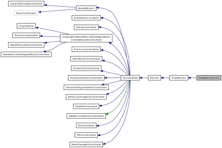
The diagram in Fig. 1 also shows the extensive use of inheritance, especially multiple inheritance for interfaces, employed by the MOOSE framework. In this context, the “interface” classes have almost no data, and are used to provide access to the various MOOSE systems (Functions, UserObjects, Postprocessors, pseudorandom numbers, etc.) within Kernels. Each Kernel also “is a” (in the object-oriented sense) MooseObject, which allows it to be stored polymorphically in collections of other MooseObjects, and used in a generic manner. Finally, we note that inheriting from the Coupleable interface allows Kernels for a given equation to depend on the other variables in the system of equations, which is essential for multiphysics applications.

⬇

1// framework/include/kernels/TimeDerivative.h

2class TimeDerivative : public TimeKernel

3{

4public:

5 TimeDerivative(const InputParameters & parameters);

6 virtual void computeJacobian() override;

7protected:

8 virtual Real computeQpResidual() override;

9 virtual Real computeQpJacobian() override;

10};

Listing 1: TimeDerivative base class public and protected interfaces.

The public and protected interfaces for the TimeDerivative base class are shown in Listing 1. There are three virtual interfaces which override the behavior of the parent TimeKernel class: computeJacobian(), computeQpResidual(), and computeQpJacobian(). The latter two functions are designed to be called at each quadrature point (as the names suggest) and have default implementations which are suitable for standard finite element problems. As will be discussed momentarily, these functions can also be customized and/or reused in specialized applications.

The computeJacobian() function, which is shown in abbreviated form in Listing 2, consists of the loops over shape functions and quadrature points necessary for assembling a single element’s Jacobian contribution into the ke variable. This listing shows where the computeQpJacobian() function is called in the body of the loop, as well as where the element Jacobian/quadrature weight (_JxW), and coordinate transformation value (_coord, used in e.g. axisymmetric simulations) are all multiplied together. Although this assembly loop is not typically overridden in MOOSE codes, the possibility nevertheless exists to do so.

⬇

1// framework/src/kernels/TimeDerivative.C

2void

3TimeDerivative::computeJacobian()

4{

5 DenseMatrix<Number> & ke = _assembly.jacobianBlock(_var.number(), _var.number());

6

7 for (_i = 0; _i < _test.size(); _i++)

8 for (_j = 0; _j < _phi.size(); _j++)

9 for (_qp = 0; _qp < _qrule->n_points(); _qp++)

10 ke(_i, _i) += _JxW[_qp] * _coord[_qp] * computeQpJacobian();

11}

Listing 2: TimeDerivative::computeJacobian() definition.

Moving on to the navier_stokes module, we next consider the implementation of the INSMomentumTimeDerivative class itself, which is shown in Listing 3. From the listing, we observe that this class inherits the TimeDerivative class from the framework, and overrides three interfaces from that class: computeQpResidual(), computeQpJacobian(), and computeQpOffDiagJacobian(). These overrides are the mechanism by which the framework implementations are customized to simulate the INS equations. Since (59) and (60) also involve the fluid density $\rho$, this class manages a constant reference to a MaterialProperty, _rho, that can be used at each quadrature point.

⬇

1// modules/navier_stokes/include/kernels/INSMomentumTimeDerivative.h

2class INSMomentumTimeDerivative : public TimeDerivative

3{

4public:

5 INSMomentumTimeDerivative(const InputParameters & parameters);

6

7protected:

8 virtual Real computeQpResidual() override;

9 virtual Real computeQpJacobian() override;

10 virtual Real computeQpOffDiagJacobian(unsigned jvar) override;

11

12 // Parameters

13 const MaterialProperty<Real> & _rho;

14};

Listing 3: INSMomentumTimeDerivative class methods.

The implementation of the specialized computeQpResidual() and computeQpJacobian() functions of the INSMomentumTimeDerivative class are shown in Listing 4. The only difference between the base class and specialized implementations is multiplication by the material property $\rho$, so the derived class implementations are able to reuse code by calling the base class methods directly. Although this example is particularly simple, the basic ideas extend to the other Kernels, boundary conditions, Postprocessors, etc. used in the navier_stokes module. In §4.2, we go into a bit more detail about the overall design of the INS Kernels, while continuing to highlight the manner in which C⁺⁺ language features are used to encourage code reuse and minimize code duplication.

⬇

1// modules/navier_stokes/src/kernels/INSMomentumTimeDerivative.C

2Real

3INSMomentumTimeDerivative::computeQpResidual()

4{

5 return _rho[_qp] * TimeDerivative::computeQpResidual();

6}

7

8Real

9INSMomentumTimeDerivative::computeQpJacobian()

10{

11 return _rho[_qp] * TimeDerivative::computeQpJacobian();

12}

Listing 4: INSMomentumTimeDerivative implementations showing relation to the base TimeDerivative class methods.

4.2 Navier–Stokes module Kernel design

All INS kernels, regardless of whether they contribute to the mass or momentum equation residuals, inherit from the INSBase class whose interface is partially shown in Listing 5. This approach reduces code duplication since both the momentum and mass equation stabilization terms (SUPG and PSPG terms, respectively) require access to the strong form of the momentum equation residual.

Residual contributions which have been integrated by parts are labeled with the “weak” descriptor in the INSBase class, while the non-integrated-by-parts terms have the “strong” descriptor. Methods with a “d” prefix are used for computing Jacobian contributions. Several of the INSBase functions return RealVectorValue objects, which are vectors of length $n_{s}$ that have mathematical operations (inner products, norms, etc.) defined on them.

⬇

1// modules/navier_stokes/include/kernels/INSBase.h

2class INSBase : public Kernel

3{

4public:

5 INSBase(const InputParameters & parameters);

6

7protected:

8 virtual RealVectorValue convectiveTerm();

9 virtual RealVectorValue dConvecDUComp(unsigned comp);

10

11 virtual RealVectorValue strongViscousTermLaplace();

12 virtual RealVectorValue strongViscousTermTraction();

13 virtual RealVectorValue dStrongViscDUCompLaplace(unsigned comp);

14 virtual RealVectorValue dStrongViscDUCompTraction(unsigned comp);

15

16 virtual RealVectorValue weakViscousTermLaplace(unsigned comp);

17 virtual RealVectorValue weakViscousTermTraction(unsigned comp);

18 virtual RealVectorValue dWeakViscDUCompLaplace();

19 virtual RealVectorValue dWeakViscDUCompTraction();

20

21 virtual RealVectorValue strongPressureTerm();

22 virtual Real weakPressureTerm();

23 virtual RealVectorValue dStrongPressureDPressure();

24 virtual Real dWeakPressureDPressure();

25};

Listing 5: Partial listing of INSBase class methods.

The inheritance diagram for the INSBase class is shown in Fig. 2. The Advection, AdvectionSUPG, and BodyForceSUPG Kernels are specific to the scalar advection equation, while the INSMass and INSMomentumBase classes are used in simulations of the INS equations. INSMomentumBase is not invoked directly in applications, instead one of the four subclasses, INSMomentumLaplaceForm, INSMomentumTractionForm, INSMomentumLaplaceFormRZ, and INSMomentumTractionFormRZ must be used, depending on what coordinate system and viscous term form is employed. INSMomentumBase is a so-called abstract base class, which is indicated by the =0 syntax on various functions in Listing 6.

Figure 2: Inheritance diagram for INS Kernels in the navier_stokes module.

⬇

1// modules/navier_stokes/include/kernels/INSMomentumBase.h

2class INSMomentumBase : public INSBase

3{

4public:

5 INSMomentumBase(const InputParameters & parameters);

6

7protected:

8 virtual Real computeQpResidual();

9 virtual Real computeQpJacobian();

10 virtual Real computeQpOffDiagJacobian(unsigned jvar);

11 virtual Real computeQpResidualViscousPart() = 0;

12 virtual Real computeQpJacobianViscousPart() = 0;

13 virtual Real computeQpOffDiagJacobianViscousPart(unsigned jvar) = 0;

14};

Listing 6: Partial listing of INSMomentumBase class members.

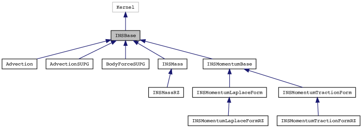
Recalling (15) and (21), the main difference between the Laplace and traction forms of the momentum equation are in the viscous term. Therefore, computeQpResidualViscousPart(), computeQpJacobianViscousPart(), and computeQpOffDiagJacobianViscousPart() are left unspecified in the INSMomentumBase class. The basic idea behind this design is to let the derived classes, INSMomentumLaplaceForm and INSMomentumTractionForm, specialize these functions. The specialized functions for the Laplace version are shown in Listing 7. We note in particular that the off-diagonal contribution (Jacobian contributions due to variables other than the one the current Kernel is acting on) is zero for this form of the viscous term.

⬇

1// modules/navier_stokes/src/kernels/INSMomentumLaplaceForm.C

2Real

3INSMomentumLaplaceForm::computeQpResidualViscousPart()

4{

5 return _mu[_qp] * (_grad_u[_qp] * _grad_test[_i][_qp]);

6}

7

8Real

9INSMomentumLaplaceForm::computeQpJacobianViscousPart()

10{

11 return _mu[_qp] * (_grad_phi[_j][_qp] * _grad_test[_i][_qp]);

12}

13

14Real

15INSMomentumLaplaceForm::computeQpOffDiagJacobianViscousPart(unsigned /*jvar*/)

16{

17 return 0.;

18}

Listing 7: Pure virtual INSMomentumBase members overridden by the INSMomentumLaplaceForm subclass.

Finally, as will be discussed in §6.2, the INSMassRZ, INSMomentumLaplaceFormRZ, and INSMomentumTractionFormRZ Kernels implement additional terms which appear in the axisymmetric form of the governing equations. In this case, the object of the inheritance structure shown in Fig. 2 is not for derived classes to override their base class functionality, but instead to append to it. The implementation is therefore analogous to the way in which the INSMomentumTimeDerivative class explicitly calls methods from the base TimeDerivative class.

4.3 Sample input file

The primary way in which users construct and customize MOOSE-based simulations is by creating and modifying text-based input files. These files can be developed using either a text editor (preferably one which can be extended to include application-specific syntax highlighting and keyword suggestion/auto completion such as Atom) or via the MOOSE GUI, which is known as Peacock. In this section, we describe in some detail the structure of an input file that will be subsequently used in §6.3 to compute the three-dimensional flow field over a sphere.

The first part of the input file in question is shown in Listing 8. The file begins by defining the mu and rho variables which correspond to the viscosity and density of the fluid, respectively, and can be used to fix the Reynolds number for the problem. These variables, which do not appear in a named section (regions demarcated by square brackets) are employed in a preprocessing step by the input file parser based on a syntax known as “dollar bracket expressions” or DBEs. As we will see subsequently in Listing 10, the expressions ${mu} and ${rho} are replaced by the specified numbers everywhere they appear in the input file, before any other parsing takes place.

⬇

1# Automatic substitution variables

2mu=4e-3

3rho=1

4

5[GlobalParams]

6 # Variable coupling and naming

7 u = vel_x

8 v = vel_y

9 w = vel_z

10 p = p

11

12 # Stabilization parameters

13 supg = true

14 pspg = true

15 alpha = 1e0

16

17 # Problem coefficients

18 gravity = ’0 0 0’

19

20 # Weak form customization

21 convective_term = true

22 integrate_p_by_parts = true

23 transient_term = true

24 laplace = true

25[]

Listing 8: [GlobalParams] section for the “flow over a sphere” problem solved in §6.3. This initial part of the input file is used to customize the weak form that will be solved and set constants common to all other input file sections.

The substitution variables are followed by the [GlobalParams] section, which contains key/value pairs that will be used (if applicable) in all of the other input file sections. In this example, we use the [GlobalParams] section to turn on the SUPG and PSPG stabilization contributions, declare variable coupling which is common to all Kernels, and customize the weak formulation by e.g. turning on/off the convective and transient terms, and toggling whether the pressure gradient term in the momentum equations is integrated by parts. Specifying the variable name mapping, i.e. u = vel_x, gives the user control over the way variables are named in output files, and the flexibility to couple together different sets of equations while avoiding name collisions and the need to recompile the code.

⬇

1[Kernels]

2 # continuity equation

3 [./mass]

4 type = INSMass

5 variable = p

6 [../]

7

8 # x1-momentum equation

9 [./x_time]

10 type = INSMomentumTimeDerivative

11 variable = vel_x

12 [../]

13 [./x_momentum_space]

14 type = INSMomentumLaplaceForm

15 variable = vel_x

16 component = 0

17 [../]

18

19 # additional kernels...

20[]

Listing 9: Kernels for the “flow over a sphere” problem described in §6.3.

The next input file section, [Kernels], is shown in Listing 9. This section controls both which Kernels are built for the simulation, and which equation each Kernel corresponds to. In the navier_stokes module, the temporal and spatial parts of the momentum equations are split into separate Kernels to allow the user to flexibly define either transient or steady state simulations. In each case, the type key corresponds to a C⁺⁺ class name that has been registered with MOOSE at compile time, and the variable key designates the equation a particular Kernel applies to.

The INSMomentumLaplaceForm Kernel also has a component key which is used to specify whether the Kernel applies to the $x_{1}$, $x_{2}$, or $x_{3}$-momentum equation. In this input file snippet, only the Kernel for $x_{1}$-momentum equation is shown; the actual input file has similar sections corresponding to the other spatial directions. This design allows multiple copies of the same underlying Kernel code to be used in a dimension-agnostic way within the simulation. Finally, we note that the size of the input file can be reduced through the use of custom MOOSE Actions which are capable of adding Variables, Kernels, BCs, etc. to the simulation programmatically, although this is an advanced approach which is not discussed in detail here.

Listing 10 shows the [Functions], [BCs], and [Materials] blocks from the same input file. In the [Functions] block, a ParsedFunction named “inlet_func” is declared. In MOOSE, ParsedFunctions are constructed from strings of standard mathematical expressions such as sqrt, *, /, ^, etc. These strings are parsed, optimized, and compiled at runtime, and can be called at required spatial locations and times during the simulation (the characters x, y, z, and t in such strings are automatically treated as spatiotemporal coordinates in MOOSE). In the spherical flow application, inlet_func is used in the vel_z_inlet block of the [BCs] section to specify a parabolic inflow profile in the $x_{3}$-direction. The boundary condition which imposes this inlet profile is of type FunctionDirichletBC, and it acts on the vel_z variable, which corresponds to the $x_{3}$ component of the velocity.

⬇

1[Functions]

2 [./inlet_func]

3 type = ParsedFunction

4 value = ’sqrt((x-2)^2 * (x+2)^2 * (y-2)^2 * (y+2)^2) / 16’

5 [../]

6[]

7

8[BCs]

9 [./vel_z_inlet]

10 type = FunctionDirichletBC

11 function = inlet_func

12 variable = vel_z

13 boundary = inlet

14 [../]

15

16 # additional bcs...

17[]

18

19[Materials]

20 [./const]

21 type = GenericConstantMaterial

22 prop_names = ’rho mu’

23 prop_values = ’${rho} ${mu}’

24 [../]

25[]

Listing 10: [Functions], [BCs], and [Materials] blocks for the “flow over a sphere” problem described in §6.3.

The last section of Listing 10 shows the [Materials] block for the spherical flow problem. In MOOSE, material properties can be understood generically as “quadrature point quantities,” that is, values that are computed independently at each quadrature point and used in the finite element assembly routines. In general they can depend on the current solution and other auxiliary variables computed during the simulation, but in this application the material properties are simply constant. Therefore, they are implemented using the correspondingly simple GenericConstantMaterial class which is built in to MOOSE. GenericConstantMaterial requires the user to provide two input parameter lists named prop_names and prop_values, which contain, respectively, the names of the material properties being defined and their numerical values. In this case, the numerical values are provided by the dollar bracket expressions ${rho} and ${mu}, which the input file parser replaces with the numerical values specified at the top of the file.

Listing 11 details the [Executioner] section of the sphere flow input file. This is the input file section where the time integration scheme is declared and customized, and the solver parameters, tolerances, and iteration limits are defined. For the sphere flow problem, we employ a Transient Executioner which will perform num_steps = 100 timesteps using an initial timestep of $\Delta t=0.5$. Since no specific time integration scheme is specified, the MOOSE default, first-order implicit Euler time integration, will be used. If the nonlinear solver fails to converge for a particular timestep, MOOSE will automatically decrease $\Delta t$ by a factor of $1/2$ and retry the most recent solve until a timestep smaller than dtmin is reached, at which point the simulation will exit with an appropriate error message.

Adaptive timestep selection is controlled by the IterationAdaptiveDT TimeStepper. For this TimeStepper, the user specifies an optimal_iterations number corresponding to their desired number of Newton steps per timestep. If the current timestep requires fewer than optimal_iterations to converge, the timestep is increased by an amount proportional to the growth_factor parameter, otherwise the timestep is shrunk by an amount proportional to the cutback_factor. Use of this TimeStepper helps to efficiently and robustly drive the simulation to steady state, but does not provide any rigorous guarantees of local or global temporal error control.

⬇

1[Executioner]

2 # TimeIntegrator and TimeStepper customization

3 type = Transient

4 num_steps = 100

5 trans_ss_check = true

6 ss_check_tol = 1e-10

7 dtmin = 5e-4

8 dt = .5

9 [./TimeStepper]

10 dt = .5

11 type = IterationAdaptiveDT

12 cutback_factor = 0.4

13 growth_factor = 1.2

14 optimal_iterations = 5

15 [../]

16

17 # Solver tolerances and iteration limits

18 nl_rel_tol = 1e-8

19 nl_abs_tol = 1e-12

20 nl_max_its = 10

21 l_tol = 1e-6

22 l_max_its = 10

23 line_search = ’none’

24

25 # Options passed directly to PETSc

26 petsc_options = ’-snes_converged_reason -ksp_converged_reason’

27 petsc_options_iname = ’-pc_type -pc_factor_shift_type -pc_factor_mat_solver_package’

28 petsc_options_value = ’lu NONZERO superlu_dist’

29[]

Listing 11: The [Executioner] blocks for the “flow over a sphere” problem described in §6.3.

Finally, we discuss a few of the linear and nonlinear solver tolerances that can be controlled by parameters specified in the [Executioner] block. The Newton solver’s behavior is primarily governed by the nl_rel_tol, nl_abs_tol, and nl_max_its parameters, which set the required relative and absolute residual norm reductions (the solve stops if either one of these tolerances is met) and the maximum allowed number of nonlinear iterations, respectively, for the nonlinear solve. The l_tol and l_max_its parameters set the corresponding values for the linear solves which occur at each nonlinear iteration, and the line_search parameter can be used to specify the line searching algorithm employed by the nonlinear solver; the possible options are described in §3.4.

The petsc_options, petsc_options_iname, and petsc_options_value parameters are used to specify command line options that are passed directly to PETSc. The first is used to specify PETSc command line options that don’t have a corresponding value, while the second two are used to specify lists of key/value pairs that must be passed to PETSc together. This particular input file gives the PETSc command line arguments required to set up a specific type of direct solver, but because almost all of PETSc’s behavior is controllable via the command line, these parameters provide a very flexible and traceable (since most input files are maintained with version control software) approach for exerting fine-grained control over the solver.

5 Verification tests

In this section, we discuss several verification tests that are available in the navier_stokes module. These tests were used in the development of the software, and versions of them are routinely run in support of continuous integration testing. The tests described here include verification of the SUPG formulation for the scalar advection equation (§5.1), the SUPG/PSPG stabilized formulation of the full INS equations (§5.2) via the Method of Manufactured Solutions (MMS), and finally, in §5.3, both the PSPG-stabilized and unstabilized formulations of the INS equations based on the classical Jeffery–Hamel exact solution for two-dimensional flow in a wedge-shaped region. The images in this section and §6 were created using the Paraview [70] visualization tool.

5.1 SUPG stabilization: Scalar advection equation

To verify the SUPG implementation in a simplified setting before tackling the full INS equations, a convergence study was first conducted for the scalar advection equation:

$$\vec{a}\cdot\nabla u =f \;\in\Omega$$ (61)

$$u =g \;\in\Gamma$$ (62)

where $\vec{a}$ is a constant velocity vector and $f$ is a forcing function. For the one-dimensional case, $\Omega=[0,1]$, and $\vec{a}$ and $f$ were chosen to be:

$$\vec{a} =(1,0,0)$$ (63)

$$f =1-x^{2}$$ (64)

In two-dimensions, $\Omega=[0,1]^{2}$, and

$$\vec{a} =(1,1,0)$$ (65)

$$f =\frac{1}{10}\left(4\sin\left(\frac{\pi x}{2}\right)+4\sin(\pi y)+7\sin\left(\frac{\pi xy}{5}\right)+5\right)$$ (66)

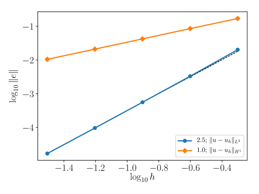
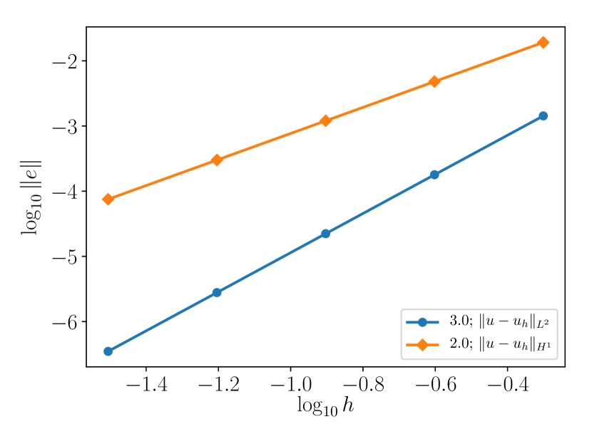
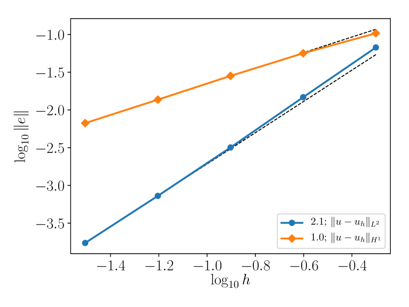
For linear ($P^{1}$) elements in 1D, nodally-exact solutions (superconvergent in the $L^{2}$-norm) are a well-known characteristic of the SUPG method [29]. We observe a convergence rate of 2.5 in this norm (see Fig. 3(a)). For quadratic ($P^{2}$) elements in 1D, convergence in the $L^{2}$-norm is generally 3rd-order unless different forms of $\tau$ are used at the vertex and middle nodes of the elements [42]. Since this specialized form of $\tau$ is currently not implemented in the navier_stokes module, we do indeed observe 3rd-order convergence, as shown in Fig. 3(b). The convergence in the $H^{1}$-norm is standard for both cases, that is, the superconvergence of the $L^{2}$-norm does not carry over to the gradients in the linear element case.

Table 1: Convergence rates, i.e. the exponent $p$ in the $O(h^{p})$ term, for the scalar advection problem with SUPG stabilization on linear and quadratic elements in 1D ($P^{1}$, $P^{2}$) and 2D ($Q^{1}$, $Q^{2}$).

	$\|u-u_{h}\|_{L^{2}(\Omega)}$	$\|u-u_{h}\|_{H^{1}(\Omega)}$
$P^{1}$	2.5	1
$P^{2}$	3	2
$Q^{1}$	2.1	1
$Q^{2}$	3	2

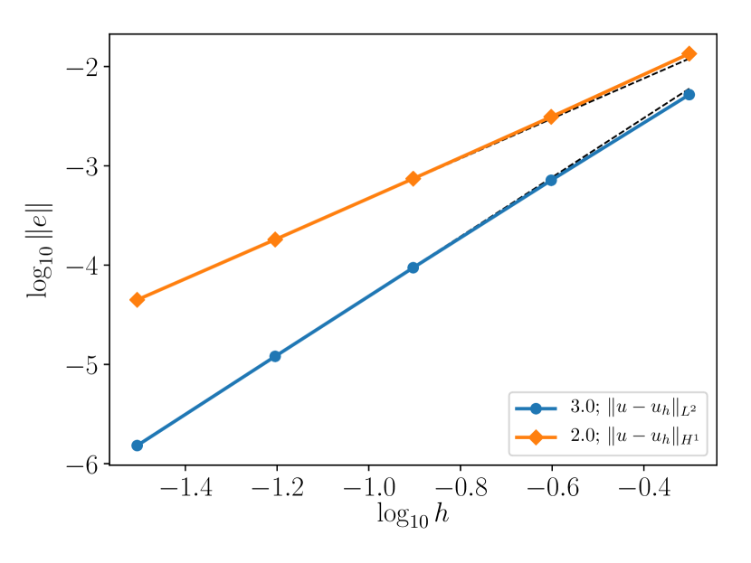
Nodally-exact/superconvergent solutions are also generally not possible in higher spatial dimensions, however the optimal rates, $O(h^{k+1})$ in $L^{2}$ and $O(h^{k})$ in $H^{1}$, are observed for both $Q^{1}$ and $Q^{2}$ elements, as shown in Fig. 4. Table 1 summarizes the convergence rates achieved for the scalar advection problem in both 1D and 2D. Given that each of the tabulated discretizations achieves at least the expected rate of convergence, we are reasonably confident that the basic approach taken in implementing this class of residual-based stabilization schemes is correct.

(a) Linear elements, 1D.

(b) Quadratic elements, 1D.

Figure 3: Convergence rates for (3(a)) $P^{1}$ and (3(b)) $P^{2}$ approximate solutions of the pure advection equation using the problem parameters given in (63) and (64).

(a) Bilinear elements, 2D.

(b) Biquadratic elements, 2D.

Figure 4: Convergence rates for (4(a)) $Q^{1}$ and (4(b)) $Q^{2}$ approximate solutions of the pure advection equation using the problem parameters given in (65) and (66).

5.2 SUPG and PSPG stabilization: INS equations

A 2D convergence verification study of the SUPG and PSPG methods was conducted via the MMS [71] using the following smooth sinusoidal functions for the manufactured solutions:

$$u_{1} =\frac{1}{10}\left(4\sin\left(\frac{\pi x}{2}\right)+4\sin(\pi y)+7\sin\left(\frac{\pi xy}{5}\right)+5\right)$$ (67)

$$u_{2} =\frac{1}{10}\left(6\sin\left(\frac{4\pi x}{5}\right)+3\sin\left(\frac{3\pi y}{10}\right)+2\sin\left(\frac{3\pi xy}{10}\right)+3\right)$$ (68)

$$p =\frac{1}{2}\left(\sin\left(\frac{\pi x}{2}\right)+2\sin\left(\frac{3\pi y}{10}\right)+\sin\left(\frac{\pi xy}{5}\right)+1\right)$$ (69)

in the unit square domain, $\Omega=[0,1]^{2}$, using the steady Laplace form of the governing equations with Dirichlet boundary conditions for all variables (including $p$) on all sides.

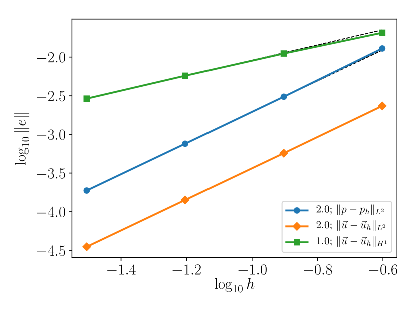
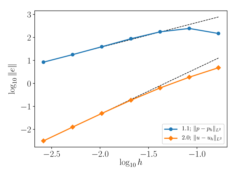
Using $Q^{1}Q^{1}$ elements in advection-dominated flows with combined SUPG and PSPG stabilization yields optimal convergence rates, as shown in the first row of Table 2. When the flow is diffusion-dominated, the pressure converges at first-order (Table 2, row 2), which is consistent with the error analysis conducted in [43] for PSPG-stabilized Stokes flow, where $\|p-p_{h}\|_{H^{1}(\Omega)}=O(h^{k-1})$ was predicted. Plots of the convergence rates for the advection- and diffusion-dominated cases can be found in Figs. 5(a) and 5(b), respectively. The advection- and diffusion-dominated cases used viscosities $\mu=1.5\times 10^{-4}$ and $\mu=15$, respectively. The element Reynolds numbers for the advection-dominated cases ranged from $7.5\times 10^{3}$ down to 469.75 as the mesh was refined, and from $7.5\times 10^{-2}$ down to $4.6875\times 10^{-3}$ for the diffusion-dominated cases.

Table 2: Convergence rates, i.e. the exponent $p$ in the $O(h^{p})$ term, for the MMS problem with SUPG and PSPG stabilization, on $Q^{1}Q^{1}$ and $Q^{2}Q^{1}$ elements, for the advection-dominated (A) and diffusion-dominated (D) problems. The results with asterisks are suboptimal based on the a priori error estimates for the linear advection-diffusion problem.

	$\|\vec{u}-\vec{u}_{h}\|_{L^{2}(\Omega)}$	$\|\vec{u}-\vec{u}_{h}\|_{H^{1}(\Omega)}$	$\|p-p_{h}\|_{L^{2}(\Omega)}$
$Q^{1}Q^{1}$ (A)	2	1	2
$Q^{1}Q^{1}$ (D)	2	1	1
$Q^{2}Q^{1}$ (A)	2∗	1∗	2
$Q^{2}Q^{1}$ (D)	3	2	2

(a) Advection-dominated.

(b) Diffusion-dominated.

Figure 5: Convergence rates for the (5(a)) advection-dominated and (5(b)) diffusion-dominated INS equations using $Q^{1}Q^{1}$ elements with both SUPG and PSPG stabilization.

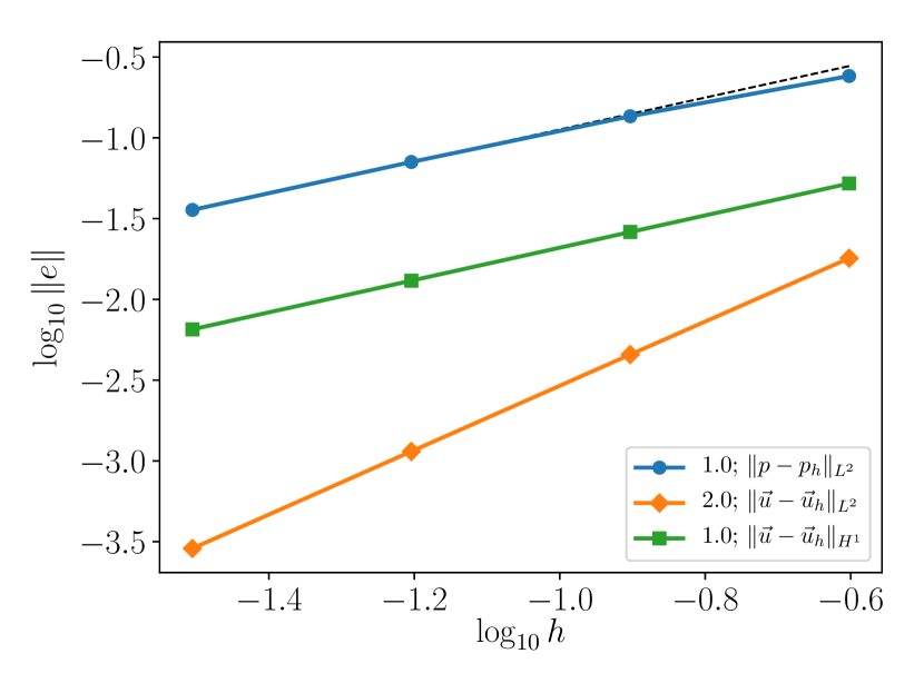
Convergence studies were also conducted using LBB-stable $Q^{2}Q^{1}$ elements with SUPG stabilization. For diffusion-dominated flows, the convergence rates for this element are optimal (Table 2, row 4). For the advection-dominated flow regime, on the other hand, we observe a drop in the convergence rates of all norms of $\|\vec{u}-\vec{u}_{h}\|$ of a full power of $h$ (Table 2, row 3). Johnson [72] and Hughes [73] proved a priori error estimates for SUPG stabilization of the scalar advection-diffusion equation showing a half-power reduction from the optimal rate in the advection-dominated regime, but in cases such as this where the true solution is sufficiently smooth, optimal convergence is often obtained for SUPG formulations. We therefore do not have a satisfactory explanation of these results at the present time. Log-log plots for the $Q^{2}Q^{1}$ elements are given in Fig. 6(a) for the advection-dominated case, and Fig. 6(b) for the diffusion-dominated case.

(a) Advection-dominated.

(b) Diffusion-dominated.

Figure 6: Convergence rates for the (6(a)) advection-dominated and (6(b)) diffusion-dominated INS equations using $Q^{2}Q^{1}$ elements with SUPG stabilization. This element pair is LBB-stable, and therefore PSPG stabilization is not required.

5.3 Jeffery–Hamel flow

Viscous, incompressible flow in a two-dimensional wedge, frequently referred to as Jeffery–Hamel flow, is described in many references including: the original works by Jeffery [74] and Hamel [75], detailed analyses of the problem [76, 77], and treatment in fluid mechanics textbooks [8, 10]. In addition to fundamental fluid mechanics research, the Jeffery–Hamel flow is also of great utility as a validation tool for finite difference, finite element, and related numerical codes designed to solve the INS equations under more general conditions. The navier_stokes module contains a regression test corresponding to a particular Jeffery–Hamel flow configuration, primarily because it provides a verification method which is independent from the MMS described in the preceding sections.

The Jeffery–Hamel solution corresponds to flow constrained to a wedge-shaped region defined by: $r_{1}\leq r\leq r_{2}$, $-\alpha\leq\theta\leq\alpha$. The origin ($r=0$) is a singular point of the flow, and is therefore excluded from numerical computations. The governing equations are the INS mass and momentum conservation equations in cylindrical polar coordinates, under the assumption that the flow is purely radial ($u_{\theta}=0$) in nature. The boundary conditions are no slip on the solid walls ($u_{r}(r,\pm\alpha)=0$) of the wedge, and symmetry about the centerline ($\theta=0$) of the channel. Under these assumptions, it is possible to show [78] that the solution of the governing equations is:

$$u_{r} =\frac{\lambda}{r}f(\eta)$$ (70)

$$p =p^{\ast}+\frac{2\mu\lambda}{r^{2}}(f(\eta)+K)$$ (71)

where $\lambda$ is a constant with units of (length)²/time which is proportional to the centerline (maximum) velocity, $\eta\equiv\frac{\theta}{\alpha}$ is the non-dimensionalized angular coordinate, $p^{\ast}$ is an arbitrary constant, $f(\eta)$ is a dimensionless function that satisfies the third-order nonlinear ordinary differential equation (ODE)

$$f^{\prime\prime\prime}+2\text{Re}\,\alpha f\!f^{\prime}+4\alpha^{2}f^{\prime} =0\quad 0<\eta<1$$ (72)

$$f(0) =1\quad\text{(centerline velocity)}$$ (73)

$$f^{\prime}(0) =0\quad\text{(centerline symmetry)}$$ (74)

$$f(1) =0\quad\text{(no slip)}$$ (75)

where $\text{Re}\equiv\frac{\lambda\alpha}{\nu}$ is the Reynolds number and $K$ is a dimensionless constant which is given in terms of $f$ by

$$K=\frac{1}{4\alpha^{2}}\left(\frac{1}{2}f^{\prime}(1)^{2}-\frac{\alpha\text{Re}}{3}-2\alpha^{2}\right)$$ (76)

Since (72) has no simple closed-form solution in general, the standard practice is to solve this ODE numerically to high accuracy and tabulate the values for use as a reference solution in estimating the accuracy of a corresponding 2D finite element solution. The pressure is only determined up to an arbitrary constant in both the analytical and numerical formulations of this problem (we impose Dirichlet velocity boundary conditions on all boundaries in the finite element formulation). Therefore, in practice we pin a single value of the pressure on the inlet centerline to zero to constrain the non-trivial nullspace. Finally, we note that although the Jeffery–Hamel problem is naturally posed in cylindrical coordinates, we solve the problem using a Cartesian space finite element formulation in the navier_stokes module.

(a) Velocity magnitude and vectors.

(b) Pressure contours.

Figure 7: Plots of Jeffery–Hamel flow showing (7(a)) velocity magnitude and vectors, and (7(b)) pressure contours for the case $\alpha=15^{\circ}$ and $\text{Re}=30$.

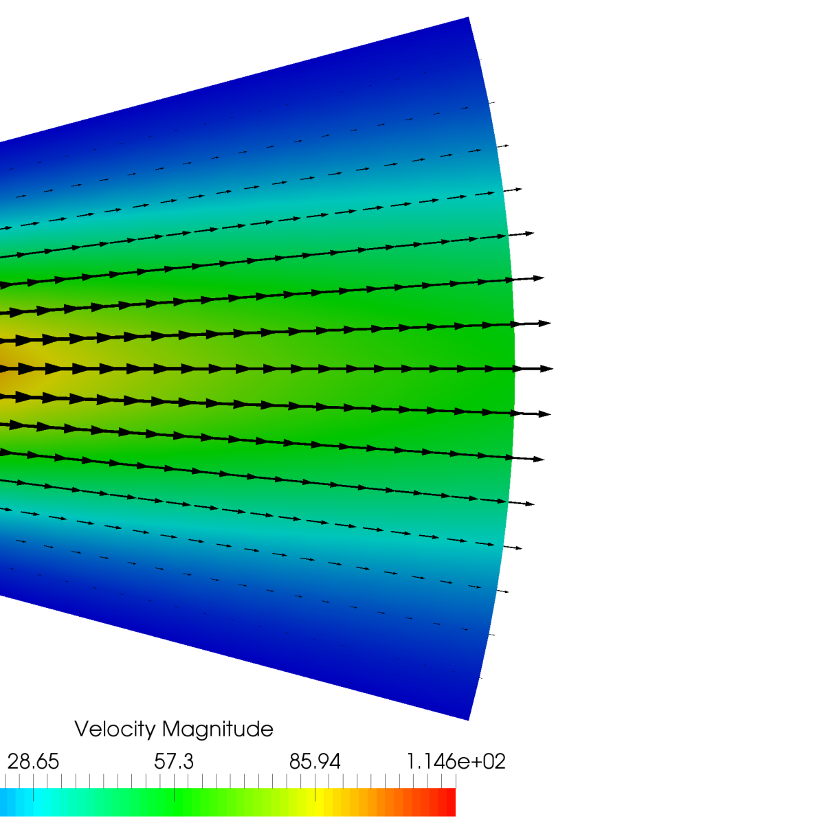
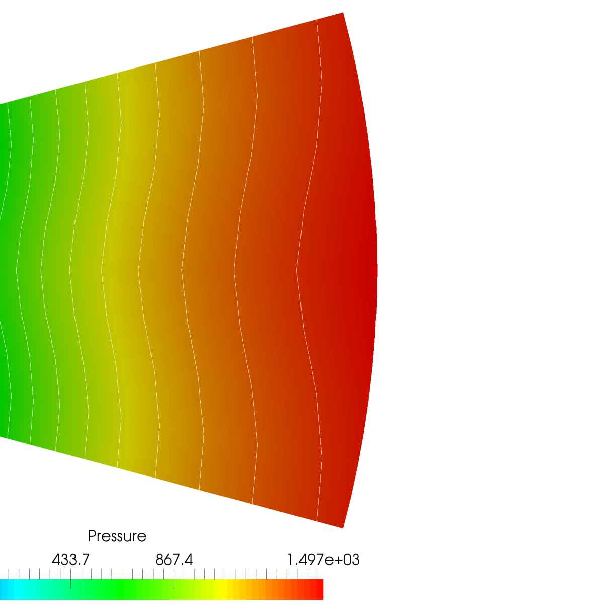
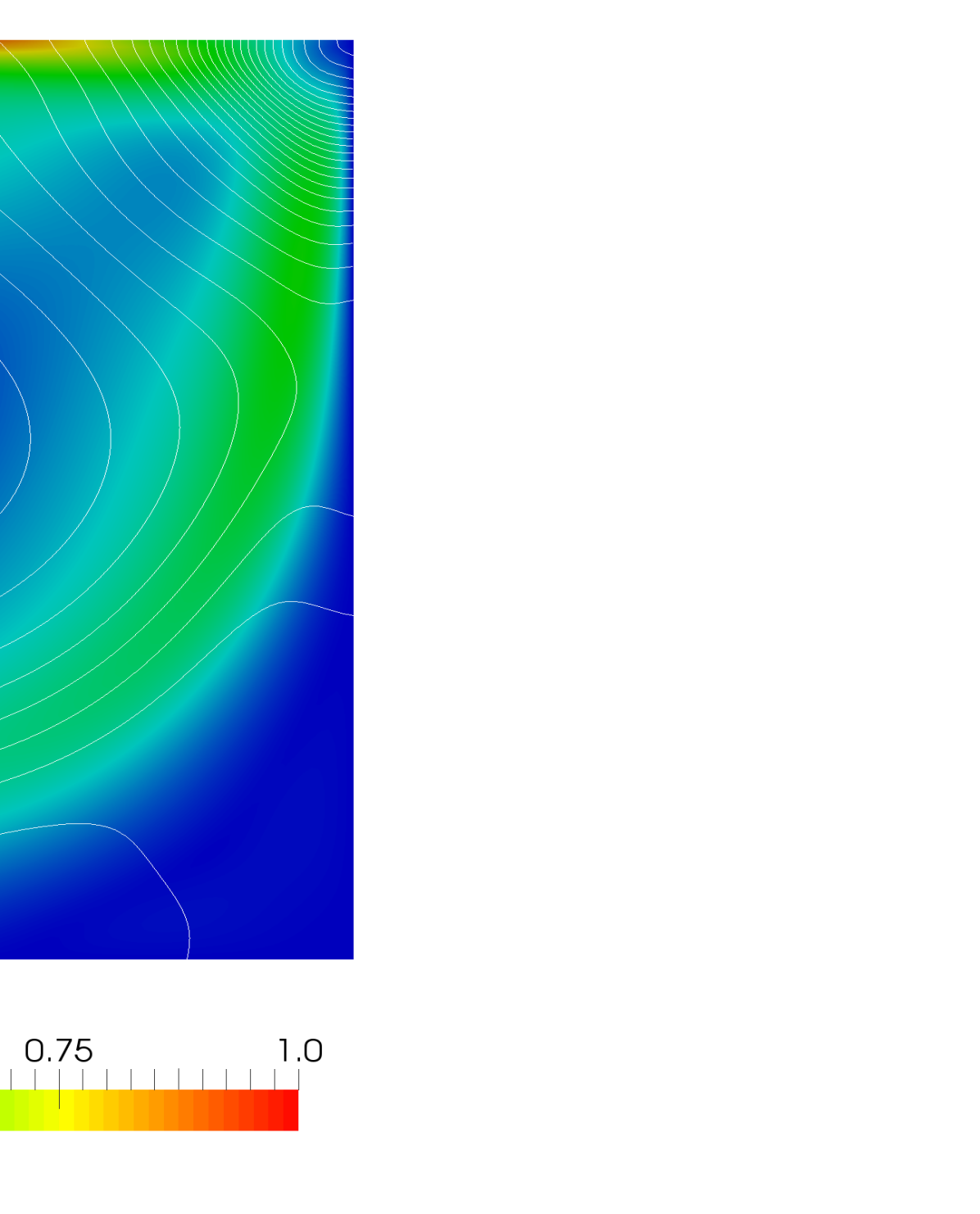
The Jeffery–Hamel velocity and pressure solutions for the particular case $\alpha=15^{\circ}$, $\text{Re}=30$, $r_{1}=1$, and $r_{2}=2$ are shown in Fig. 7. As expected from the exact solution, the flow is radially self-similar, and the centerline maximum value is proportional to $1/r$. The pressure field has a corresponding $-1/r^{2}$ dependence on the radial distance, since $K\approx-9.7822146449$ is negative in this configuration. We note that the radial flow solution is linearly unstable for configurations in which $\text{Re}\,\alpha>10.31$, since the boundary layers eventually separate and recirculation regions form due to the increasingly adverse pressure gradient. Our test case is in the linearly stable regime.

(a) PSPG-stabilized $Q^{1}Q^{1}$ elements.

(b) $Q^{2}Q^{1}$ elements.

Figure 8: Convergence rates of (8(a)) PSPG-stabilized $Q^{1}Q^{1}$ and (8(b)) $Q^{2}Q^{1}$ discretizations of the Jeffery–Hamel problem for $\alpha=15^{\circ}$ and $\text{Re}=30$.

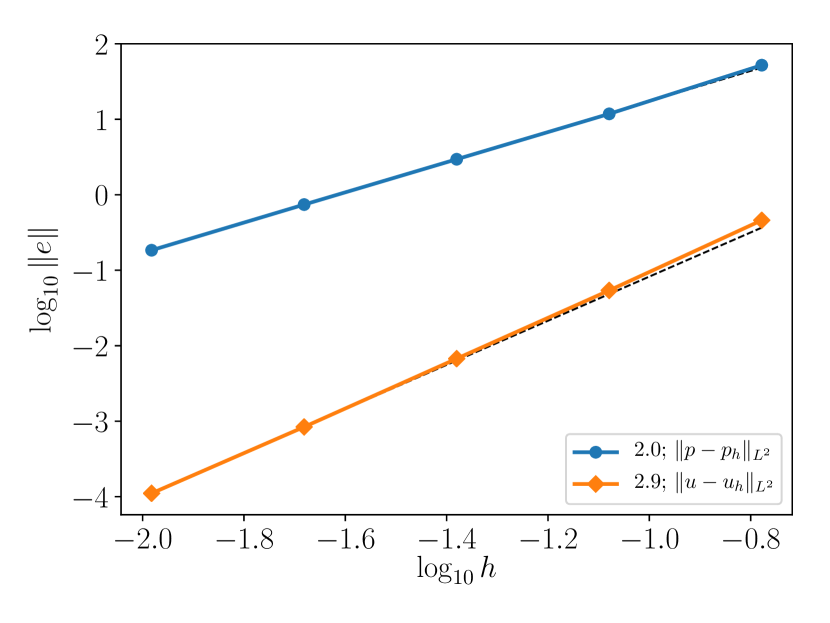
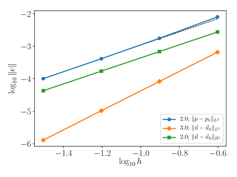
The convergence results for PSPG-stabilized $Q^{1}Q^{1}$ and unstabilized $Q^{2}Q^{1}$ finite element formulations on a sequence of uniformly-refined grids for this problem are shown in Fig. 8. Optimal rates in both the velocity and pressure are obtained for the unstabilized case, which is consistent with the diffusion-dominated results of §5.2. In the PSPG-stabilized case, the velocity converges at the optimal order, while the $\|p-p_{h}\|_{L^{2}}$ norm once again exhibits first-order convergence as in §5.2 for the diffusion-dominated problem. An interesting extension to these results would be to consider converging flow (i.e. choosing $\lambda$ and therefore $\text{Re}<0$). The converging flow configuration is linearly stable for all (negative) Reynolds numbers, and thus, for large enough negative Reynolds numbers, the numerical solution may require SUPG stabilization.

6 Representative results

In this section, we move beyond the verification tests of §5 and employ the various finite element formulations of the navier_stokes module on several representative applications. In §6.1, we report results for a “non-leaky” version of the lid-driven cavity problem at Reynolds numbers 10³ and $5\times 10^{3}$, which are in good qualitative agreement with benchmark results. Then, in §6.2, we introduce a non-Cartesian coordinate system and investigate diffusion and advection-dominated flows in a 2D expanding nozzle. Finally, in §6.3, we solve the classic problem of 3D advection-dominated flow over a spherical obstruction in a narrow channel using a hybrid mesh of prismatic and tetrahedral elements.

6.1 Lid-driven cavity

In the classic lid-driven cavity problem, the flow is induced by a moving “lid” on top of a “box” containing an incompressible, viscous fluid. In the continuous (non-leaky) version of the problem, the lid velocity is set to zero at the top left and right corners of the domain for consistency with the no-slip boundary conditions on the sides of the domain. In the present study, the computational domain is taken to be $\Omega=[0,1]^{2}$, and the lid velocity is set to:

$$u_{1}=4x(1-x)$$ (77)

while the viscosity $\mu$ is varied to simulate flows at different Reynolds numbers. Since Dirichlet boundary conditions are imposed on the entire domain, a single value of the pressure is pinned to zero in the bottom left-hand corner. We consider two representative cases of $\text{Re}=10^{3}$ and $\text{Re}=5\times 10^{3}$ in the present work, and both simulations employ an SUPG/PSPG-stabilized finite element discretization on a structured grid of $Q^{1}Q^{1}$ elements.

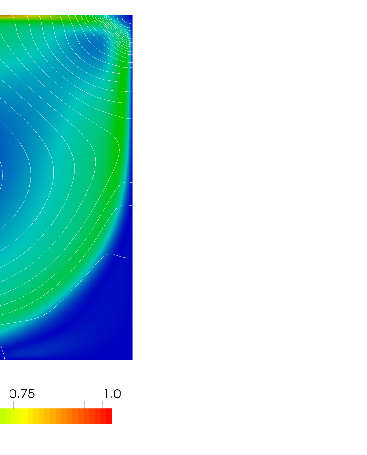
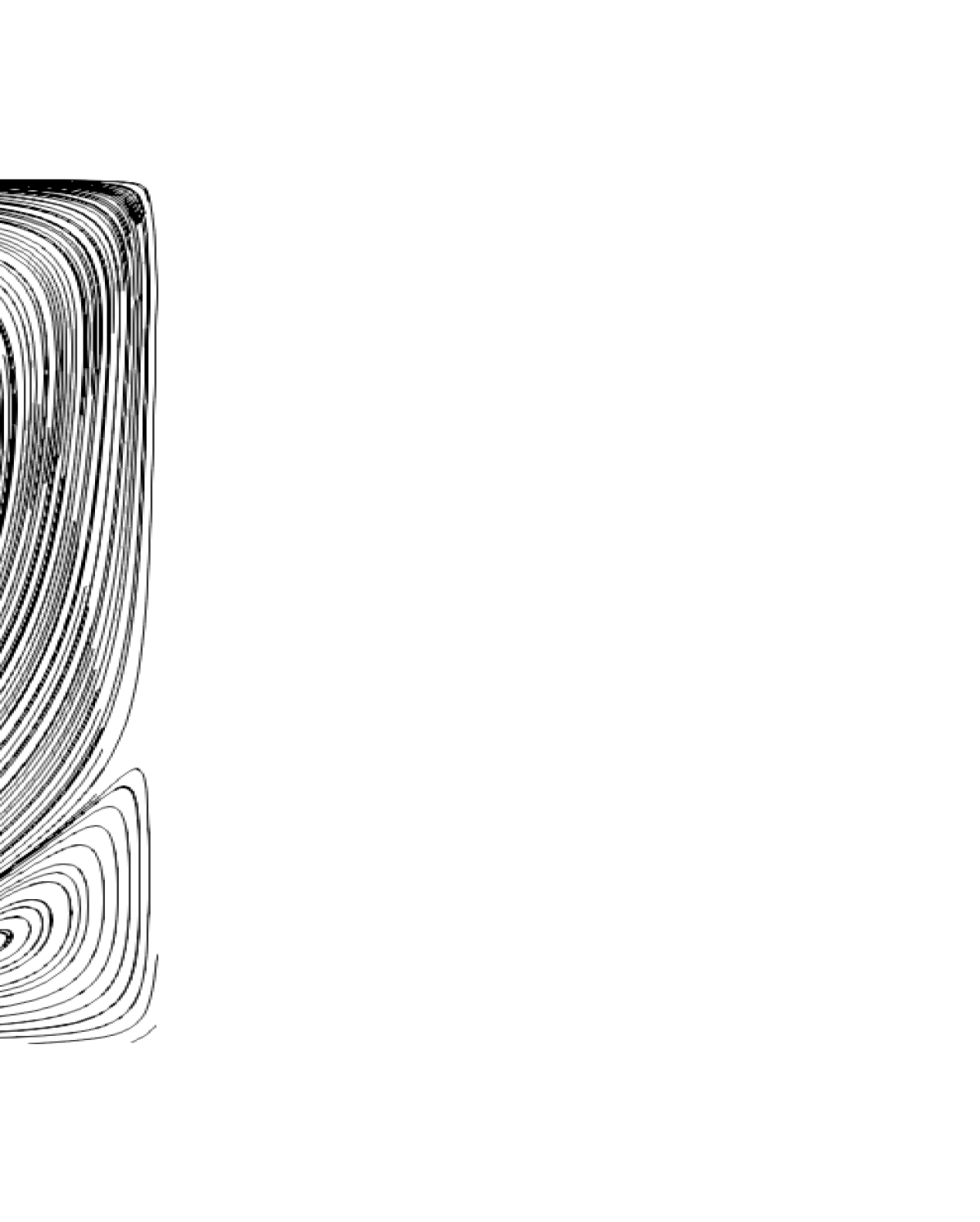
Figs. 9(a) and 9(b) show the velocity magnitude and pressure contours at steady state for the two cases, using a mesh size of $h=1/128$ in the $\text{Re}=10^{3}$ case, and $h=1/256$ in the $\text{Re}=5\times 10^{3}$ case. Solutions of the leaky version of the lid-driven cavity problem exhibit strong pressure singularities (and velocity discontinuities) in the upper corners of the domain. In contrast, for the non-leaky version of the problem solved here, the velocity field is continuous and therefore the solution has higher global regularity. Nevertheless, the pressure still varies rapidly in the upper right-hand corner of the domain (as evidenced by the closely-spaced contour lines), and fine-scale flow structures develop at high Reynolds numbers. Flow streamlines for the two problems are shown in Figs. 10(a) and 10(b). The locations and strengths of the vortices, including the appearance of a third recirculation region at $\text{Re}=5\times 10^{3}$, are consistent with the results reported in [25] and other reference works.

(a) $\text{Re}=10^{3}$, $h=1/128$.

(b) $\text{Re}=5\times 10^{3}$, $h=1/256$.

Figure 9: Pressure isobars overlaid on velocity magnitude contour plots for the lid-driven cavity problem with (9(a)) $\text{Re}=10^{3}$, $h=1/128$, and (9(b)) $\text{Re}=5\times 10^{3}$, $h=1/256$. These results are qualitatively similar to those discussed in [25] and other reference works.

(a) $\text{Re}=10^{3}$, $h=1/128$.

(b) $\text{Re}=5\times 10^{3}$, $h=1/256$.

Figure 10: Streamlines for the lid-driven cavity case with (10(a)) $\text{Re}=10^{3}$, $h=1/128$, and (10(b)) $\text{Re}=5\times 10^{3}$, $h=1/256$. The third region of recirculating flow present in the $\text{Re}=5\times 10^{3}$ result is consistent with other lid-driven cavity reference solutions.

6.2 Axisymmetric channel

To derive the axisymmetric version of the governing equations, we start by defining the vector $\vec{v}$ in cylindrical coordinates as

$$\vec{v}=v_{r}\hat{e}_{r}+v_{\theta}\hat{e}_{\theta}+v_{z}\hat{e}_{z}$$ (78)

for unit vectors $\hat{e}_{r}$, $\hat{e}_{\theta}$, $\hat{e}_{z}$. The divergence and gradient of $\vec{v}$ in cylindrical coordinates are then given by:

$$\text{div}\,\vec{v} \equiv\frac{1}{r}\frac{\partial\left(rv_{r}\right)}{\partial r}+\frac{1}{r}\frac{\partial v_{\theta}}{\partial\theta}+\frac{\partial v_{z}}{\partial z}$$ (79)

$$\text{grad}\,\vec{v} \equiv\begin{bmatrix}\frac{\partial v_{r}}{\partial r}&\frac{1}{r}\left(\frac{\partial v_{r}}{\partial\theta}-v_{\theta}\right)&\frac{\partial v_{r}}{\partial z}\\[6.0pt] \frac{\partial v_{\theta}}{\partial r}&\frac{1}{r}\left(\frac{\partial v_{\theta}}{\partial\theta}+v_{r}\right)&\frac{\partial v_{\theta}}{\partial z}\\[6.0pt] \frac{\partial v_{z}}{\partial r}&\frac{1}{r}\frac{\partial v_{z}}{\partial\theta}&\frac{\partial v_{z}}{\partial z}\end{bmatrix}$$ (80)

while the gradient and Laplacian of a scalar $g$ are given by

$$\text{grad}\,g \equiv\frac{\partial g}{\partial r}\hat{e}_{r}+\frac{1}{r}\frac{\partial g}{\partial\theta}\hat{e}_{\theta}+\frac{\partial g}{\partial z}\hat{e}_{z}$$ (81)

$$\text{Lap}\,g \equiv\frac{1}{r}\frac{\partial}{\partial r}\left(r\frac{\partial g}{\partial r}\right)+\frac{1}{r^{2}}\frac{\partial^{2}g}{\partial\theta^{2}}+\frac{\partial^{2}g}{\partial z^{2}}$$ (82)

respectively. Combining these definitions allows us to define the vector Laplacian operator in cylindrical coordinates as:

$$\text{Lap}\,\vec{u}\equiv\text{div}\,(\text{grad}\,\vec{u})^{T}=\begin{bmatrix}\text{Lap}\,u_{r}\\[6.0pt] \text{Lap}\,u_{\theta}\\[6.0pt] \text{Lap}\,u_{z}\end{bmatrix}+\begin{bmatrix}-\frac{2}{r^{2}}\frac{\partial u_{\theta}}{\partial\theta}-\frac{u_{r}}{r^{2}}\\[6.0pt] \phantom{-}\frac{2}{r^{2}}\frac{\partial u_{r}}{\partial\theta}-\frac{u_{\theta}}{r^{2}}\\[6.0pt] 0\end{bmatrix}$$ (83)

The axisymmetric formulation then proceeds by substituting (78)–(83) into e.g. the semi-discrete component equations (37) and (38) and then assuming the velocity, pressure and body force terms satisfy

$$u_{\theta}=\frac{\partial u_{r}}{\partial\theta}=\frac{\partial u_{z}}{\partial\theta}=\frac{\partial p}{\partial\theta}=f_{\theta}=0$$ (84)

Under these assumptions, we can ignore the $\theta$-component of (37) since it is trivially satisfied. The remaining component equations in Laplace form are (neglecting the stabilization terms and assuming natural boundary conditions for brevity):

$$\int_{\Omega^{\prime}}\left[\rho\left(\frac{\partial u_{r}}{\partial t}+u_{r}\frac{\partial u_{r}}{\partial r}+u_{z}\frac{\partial u_{r}}{\partial z}\right)\varphi_{i}-p\frac{\partial\varphi_{i}}{\partial r}\hbox{\pagecolor{red!50}$\displaystyle\mbox{}-p\frac{\varphi_{i}}{r}$}-f_{r}\varphi_{i}\right.$$

$$\left.\qquad\qquad\mbox{}+\mu\left(\frac{\partial u_{r}}{\partial r}\frac{\partial\varphi_{i}}{\partial r}+\frac{\partial u_{r}}{\partial z}\frac{\partial\varphi_{i}}{\partial z}\hbox{\pagecolor{red!50}$\displaystyle\mbox{}+\frac{u_{r}\varphi_{i}}{r^{2}}$}\right)\right]\text{d}\Omega^{\prime}=0, \quad i=1,\ldots,N$$ (85)

$$\int_{\Omega^{\prime}}\left[\rho\left(\frac{\partial u_{z}}{\partial t}+u_{r}\frac{\partial u_{z}}{\partial r}+u_{z}\frac{\partial u_{z}}{\partial z}\right)\varphi_{i}-p\frac{\partial\varphi_{i}}{\partial z}-f_{z}\varphi_{i}\right.$$

$$\left.\qquad\qquad\mbox{}+\mu\left(\frac{\partial u_{z}}{\partial r}\frac{\partial\varphi_{i}}{\partial r}+\frac{\partial u_{z}}{\partial z}\frac{\partial\varphi_{i}}{\partial z}\right)\right]\text{d}\Omega^{\prime}=0, \quad i=1,\ldots,N$$ (86)

$$\int_{\Omega^{\prime}}\left(\frac{\partial u_{r}}{\partial r}\hbox{\pagecolor{red!50}$\displaystyle\mbox{}+\frac{u_{r}}{r}$}+\frac{\partial u_{z}}{\partial z}\right)\psi_{i}\;\text{d}\Omega^{\prime}=0, \quad i=1,\ldots,M$$ (87)

Upon inspection, we note that (85)–(87) are equivalent to the two-dimensional Cartesian INS equations, except for the three additional terms which have been highlighted in red, and the factor of $r$ which arises from the $\text{d}\Omega^{\prime}=r\,\text{d}r\,\text{d}z$ terms. Therefore, to simulate axisymmetric flow in the navier_stokes module, we simply use the two-dimensional Cartesian formulation, treat the $u_{1}$ and $u_{2}$ components of the velocity as $u_{r}$ and $u_{z}$, respectively, append the highlighted terms, and multiply by $r$ when computing the element integrals.

To test the navier_stokes module’s axisymmetric simulation capability, we consider flow through a conical diffuser with inlet radius $R=1/2$ and specified velocity profile:

$$u_{r} =0$$ (88)

$$u_{z} =1-4r^{2}$$ (89)

The conical section expands to a radius of $R=1$ at $z=1$, and then the channel cross-section remains constant until the outflow boundary at $z=4$. No-slip Dirichlet boundary conditions are applied along the outer ($r=R$) wall of the channel, and a no-normal-flow ($u_{r}=0$) Dirichlet boundary condition is imposed along the channel centerline to enforce symmetry about $r=0$. As is standard for these types of problems, natural boundary conditions ($\vec{s}=\vec{0}$) are imposed at the outlet.

We note that natural boundary conditions are used here for convenience, and not because they are particularly well-suited to modeling the “real” outflow boundary. As discussed in §3.1.1, a more realistic approach would be to employ a longer channel region to ensure that the chosen outlet boundary conditions do not adversely affect the upstream characteristics of the flow. Since our intent here is primarily to demonstrate and exercise the capabilities of the navier_stokes module, no effort is made to minimize the effects of the outlet conditions. As a final verification step, we observe that integrating (89) over the inlet yields a volumetric flow rate of

$$Q=\int_{0}^{2\pi}\!\!\!\int_{0}^{R}\left(1-4r^{2}\right)r\,\text{d}r\,\text{d}\theta=\frac{\pi}{8}$$ (90)

for this case. In this example, we employ a VolumetricFlowRate Postprocessor to ensure that the mass flowing in the inlet exactly matches (to within floating point tolerances) the mass flowing out the outlet, thereby confirming the global conservation property of the FEM for the axisymmetric case.

The characteristics of the computed solutions depend strongly on the Reynolds number for this problem, which is similar in nature to the classic backward-facing step problem [79]. The flow must decelerate as it flows into the larger section of the channel, and this deceleration may be accompanied by a corresponding rise in pressure, also known as an adverse pressure gradient. If the adverse pressure gradient is strong enough (i.e. at high enough Reynolds numbers) the flow will separate from the channel wall at the sharp inlet, and regions of recirculating flow will form. At low Reynolds numbers, on the other hand, the pressure gradient will remain favorable, and flow separation will not occur.

We consider two distinct cases in the present work: a “creeping flow” case with $\text{Re}=0.5$ ($\mu=1$) and an advection-dominated case with $\text{Re}=10^{3}$ ($\mu=0.5\times 10^{-3}$) based on the average inlet velocity and inlet diameter. In the former case, we employ an LBB-stable $P^{2}P^{1}$ finite element discretization on TRI6 elements with SUPG and PSPG stabilization disabled. In the latter case, an equal-order $P^{1}P^{1}$ discretization on TRI3 elements is employed, and both SUPG and PSPG stabilization are enabled. In both cases, unstructured meshes are employed, and no special effort is expended to grade the mesh into the near-wall/boundary layer regions of the channel.

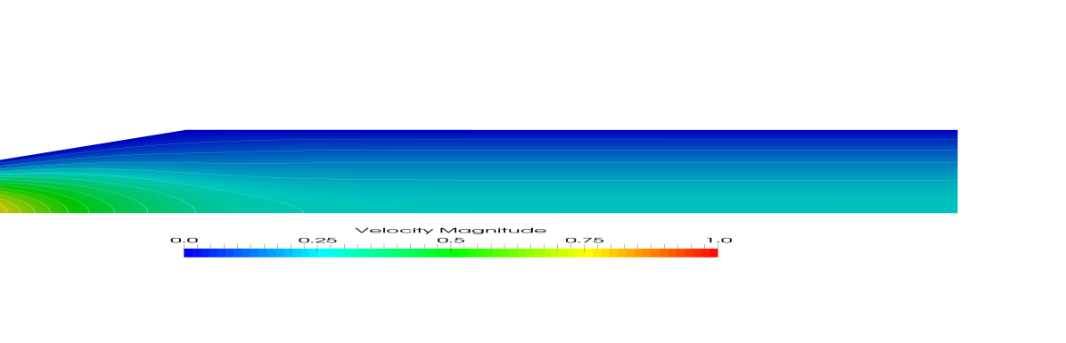
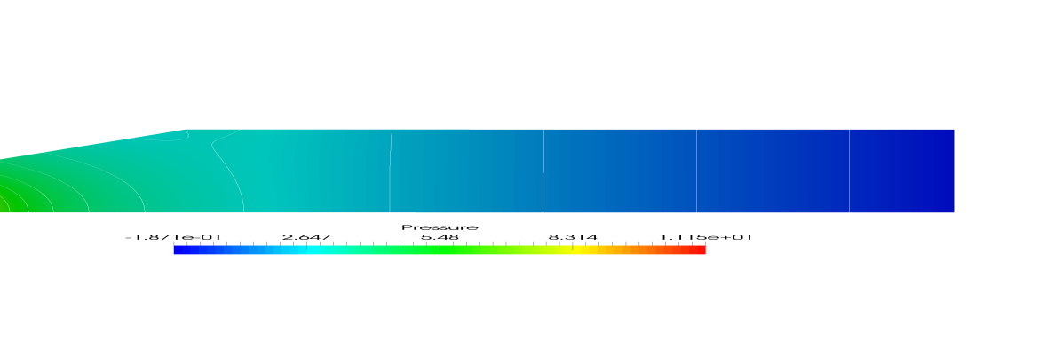
The steady state velocity magnitude and pressure contours for the diffusion-dominated case are shown in Fig. 11. In this case, we observe that the inlet velocity profile diffuses relatively quickly to a quadratic profile at the outlet, and that the flow remains attached throughout the channel. No boundary layers form, and there is a favorable, i.e. $\frac{\partial p}{\partial z}<0$, pressure gradient throughout the channel, which is disturbed only by the pressure singularity which forms at the sharp inlet. This pressure singularity is also a characteristic of backward-facing step flows, and although it reduces the overall regularity of the solution, it does not seem to have any serious negative effects on the convergence of the numerical scheme. We also remark that the downstream natural boundary conditions seem to have little effect, if any, on this creeping flow case, since the flow becomes fully-developed well before reaching the outlet.

(a) Velocity magnitude contours.

(b) Pressure contours.

Figure 11: Visualization of the axisymmetric channel flow problem showing the (11(a)) velocity magnitude and (11(b)) pressure contours for the creeping flow case ($\text{Re}=0.5$) at steady state using an unstabilized $P^{2}P^{1}$ finite element discretization on a mesh with 10102 TRI6 elements and 20513 nodes.

(a) Velocity magnitude and streamtraces.

(b) Pressure contours.

Figure 12: Advection-dominated ($\text{Re}=10^{3}$) axisymmetric channel flow problem visualization of (12(a)) velocity magnitude and streamtraces, and (12(b)) pressure contours at steady state on a mesh with 86212 TRI3 ($P^{1}P^{1}$) elements and 43588 nodes. The region of slow-moving reverse flow near the no-slip wall is clearly visible.

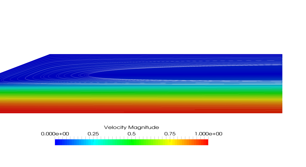
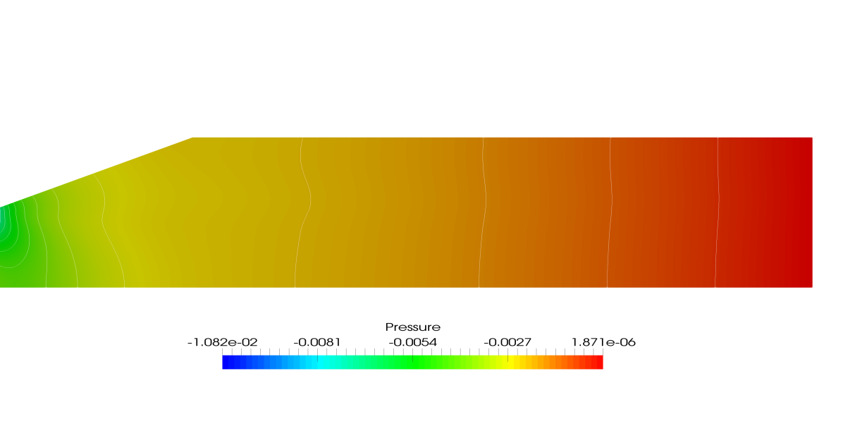
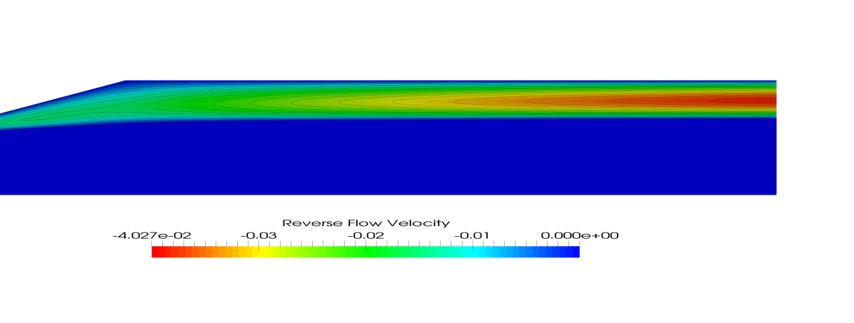
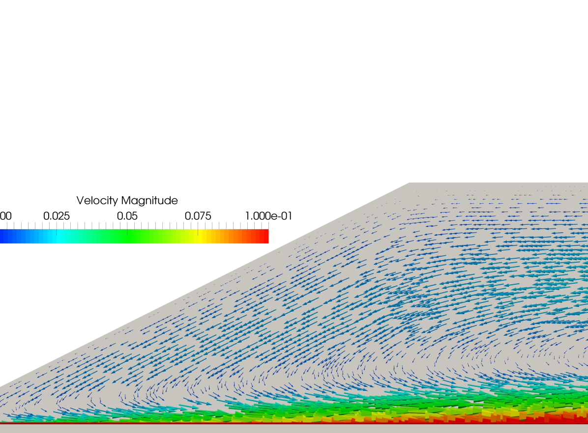
The steady state velocity magnitude, streamtraces, and pressure contours for the advection-dominated ($\text{Re}=10^{3}$) case are shown in Fig. 12. In contrast to the previous case, there is now a large region of slow, recirculating flow near the channel wall, and an adverse pressure gradient. In Fig. 13(a), the region of reversed flow is highlighted with a contour plot showing the negative longitudinal ($u_{z}$) velocities, and it seems clear that the downstream boundary condition has a much larger effect on the overall flow field in this case. In Fig. 13(b), velocity vectors in the upper half of the channel are plotted to aid in visualization of the reverse-flow region.

(a) Contours of reverse longitudinal velocity component.

(b) Near-wall velocity vectors.

Figure 13: Advection-dominated ($\text{Re}=10^{3}$) axisymmetric channel flow problem visualization of (13(a)) reverse flow velocity contours, and (13(b)) velocity vectors near the no-slip wall. Both SUPG and PSPG stabilization are used in this example.

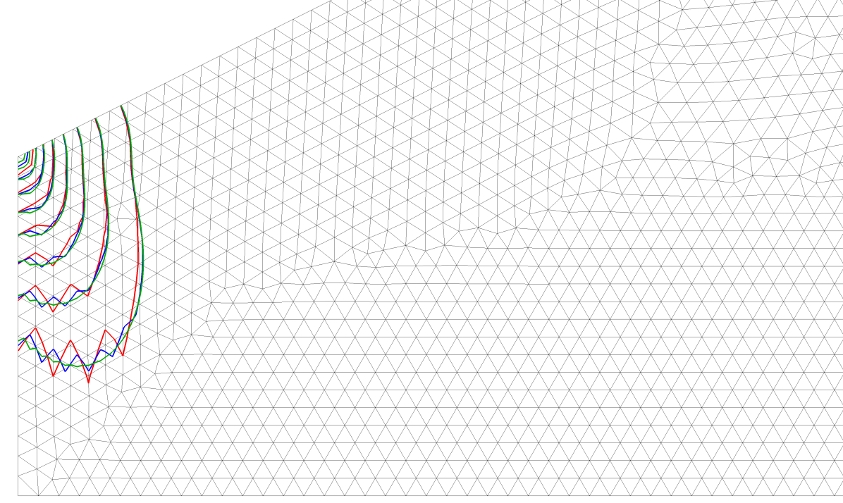
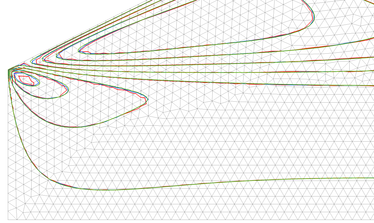
The pressure singularity is still an important characteristic of the flow in the advection-dominated case, and to investigate the error in the finite element solution near this point a small mesh convergence study was conducted on a sequence of grids with 9456, 21543, and 86212 elements. (The results in Figs. 12 and 13 are from the finest grid in this sequence.) Contour plots comparing the pressure and radial velocity near the sharp inlet corner on the different grids are given in Figs. 14(a) and 14(b), respectively. On the coarse grid (red contours) in particular, we observe pronounced non-physical oscillations in the pressure field near the singularity. These oscillations are much less prominent on the finest grid (green contours). The radial velocity contours are comparable on all three meshes, with the largest discrepancy occurring on the channel wall where the boundary layer flow separation initially occurs.

(a) $p$ contours.

(b) $u_{r}$ contours.

Figure 14: Evenly-spaced contours of (14(a)) $p\in[-1.08\times 10^{-2},-4.81\times 10^{-3}]$ and (14(b)) $u_{r}\in[-7.32\times 10^{-3},6.93\times 10^{-3}]$ on meshes with 9456 (red), 21543 (blue), and 86212 (green) elements. Non-physical oscillations can be observed in several of the pressure contours near the sharp inlet corner on the coarser grids, but they are mostly absent in the fine grid results. The velocity contours are all fairly comparable except near the separation point on the upper wall. The background mesh shown corresponds to the coarsest grid level.

6.3 Flow over a sphere

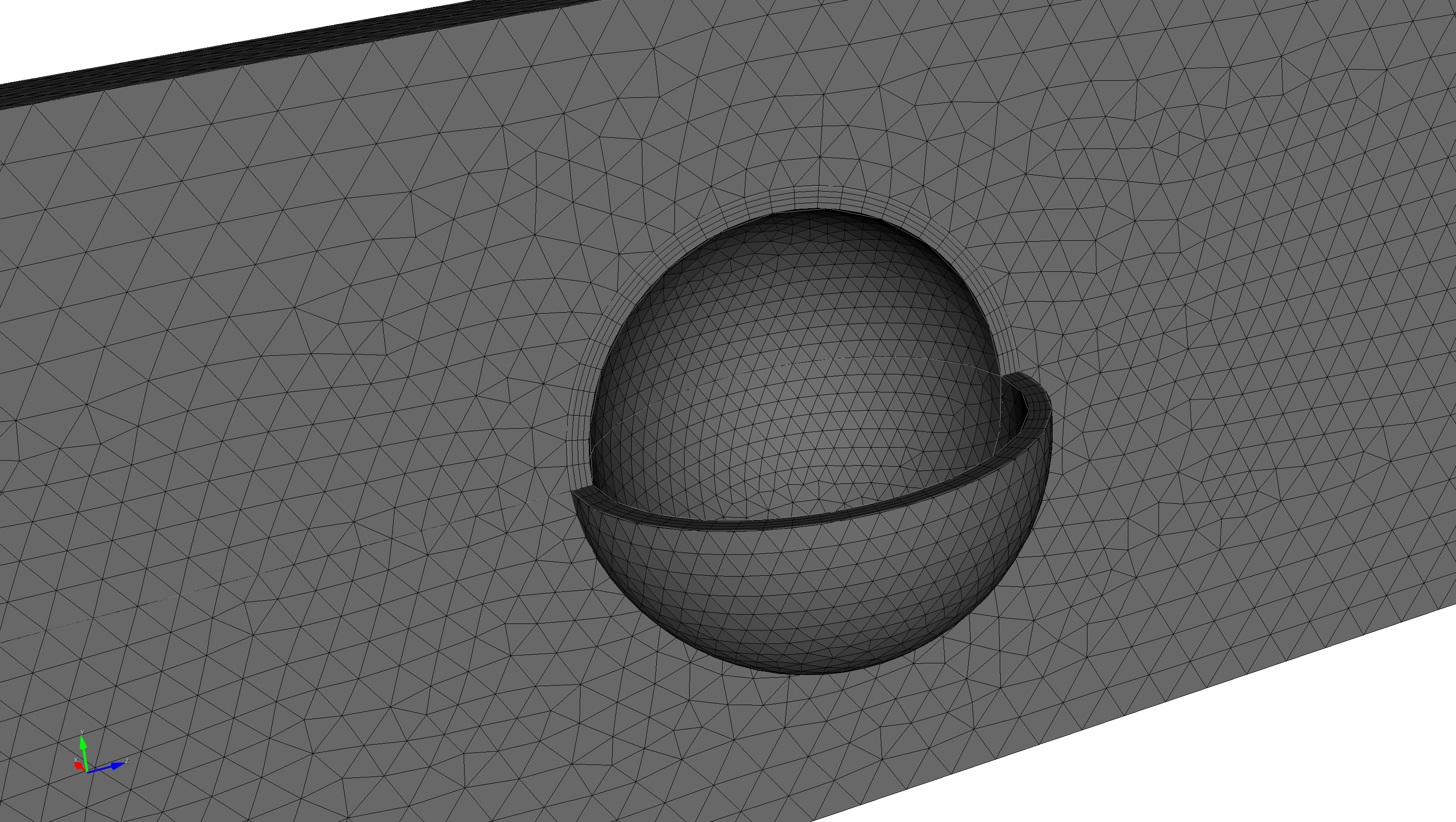
In this example, we simulate flow in the channel $\Omega=[-2,2]^{2}\times[-5,5]$ around a sphere of diameter 2 centered at the origin. The inlet flow profile is given by:

$$u_{1} =u_{2}=0$$ (91)

$$u_{3} =\frac{(4-x^{2})(4-y^{2})}{16}$$ (92)

The Reynolds number based on the maximum inlet velocity, sphere diameter, and viscosity $\mu=4\times 10^{-3}$ is $5\times 10^{2}$. (Based on the area-averaged inlet velocity, the Reynolds number is $\approx 222.22$.) A 3D hybrid mesh, pictured in Fig. 15(a), with 104069 elements (93317 tetrahedra and 10752 prisms) comprising 23407 nodes, which is locally graded near the boundary of the sphere, is used for the calculation. A transient, SUPG/PSPG-stabilized Laplace formulation of the INS equations on equal-order elements (nominally $P^{1}P^{1}$, although the prismatic elements also contain bilinear terms in the sphere-normal direction) is employed, and the equations are stepped to steady state using an implicit (backward Euler) time integration routine with adaptive timestep selection based on the number of nonlinear iterations.

Natural boundary conditions are once again imposed at the outlet. Because of the proximity of the channel walls and the outlet to the sphere, we do not necessarily expect to observe vortex shedding or non-stationary steady states even at this relatively high Reynolds number. The problem was solved in parallel on a workstation with 24 processors using Newton’s method combined with a parallel direct solver (SuperLU_DIST [80]) at each linear iteration, although an inexact Newton scheme based on a parallel Additive Schwarz preconditioner with local ILU sub-preconditioners was also found to work well.

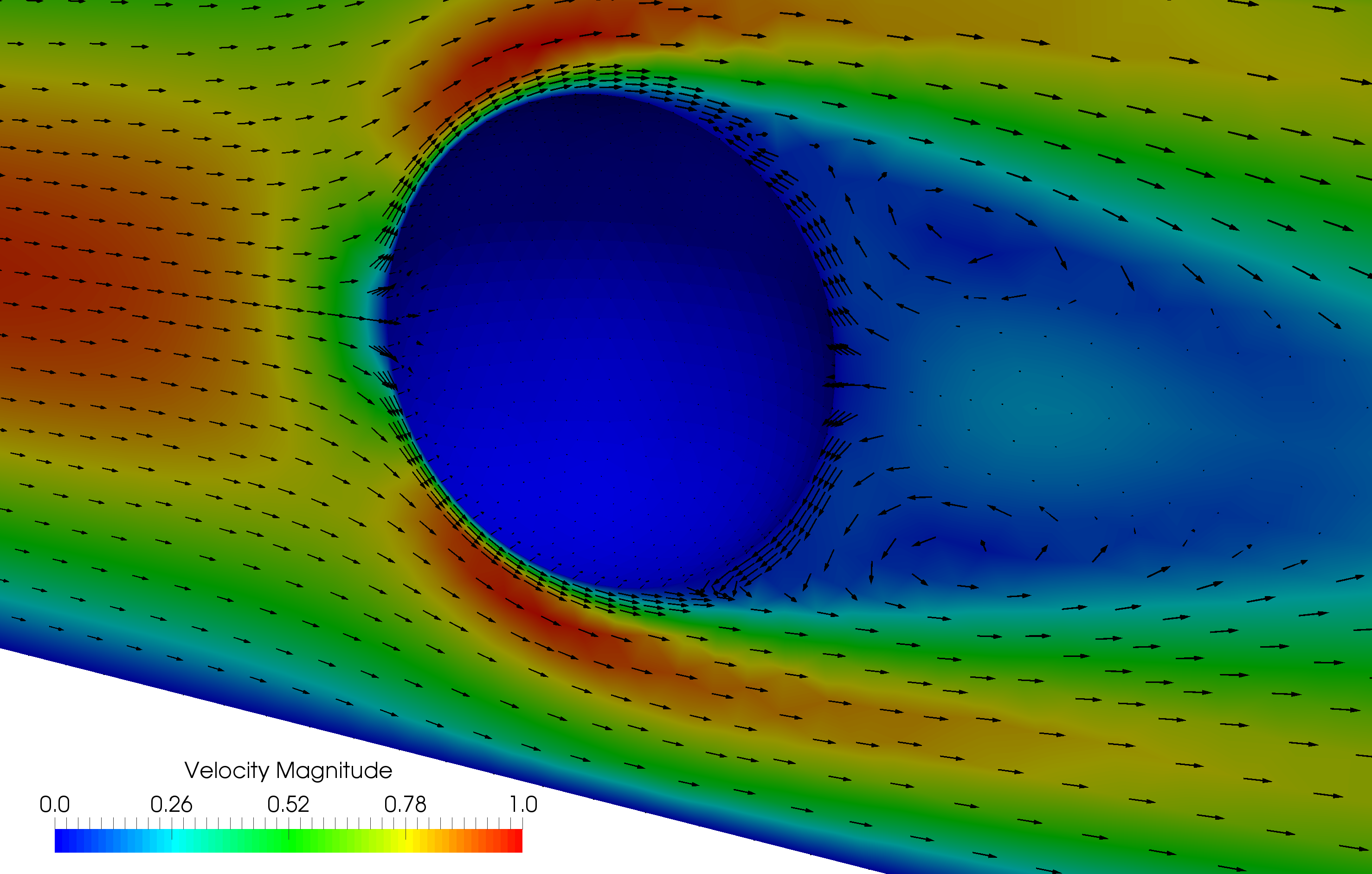
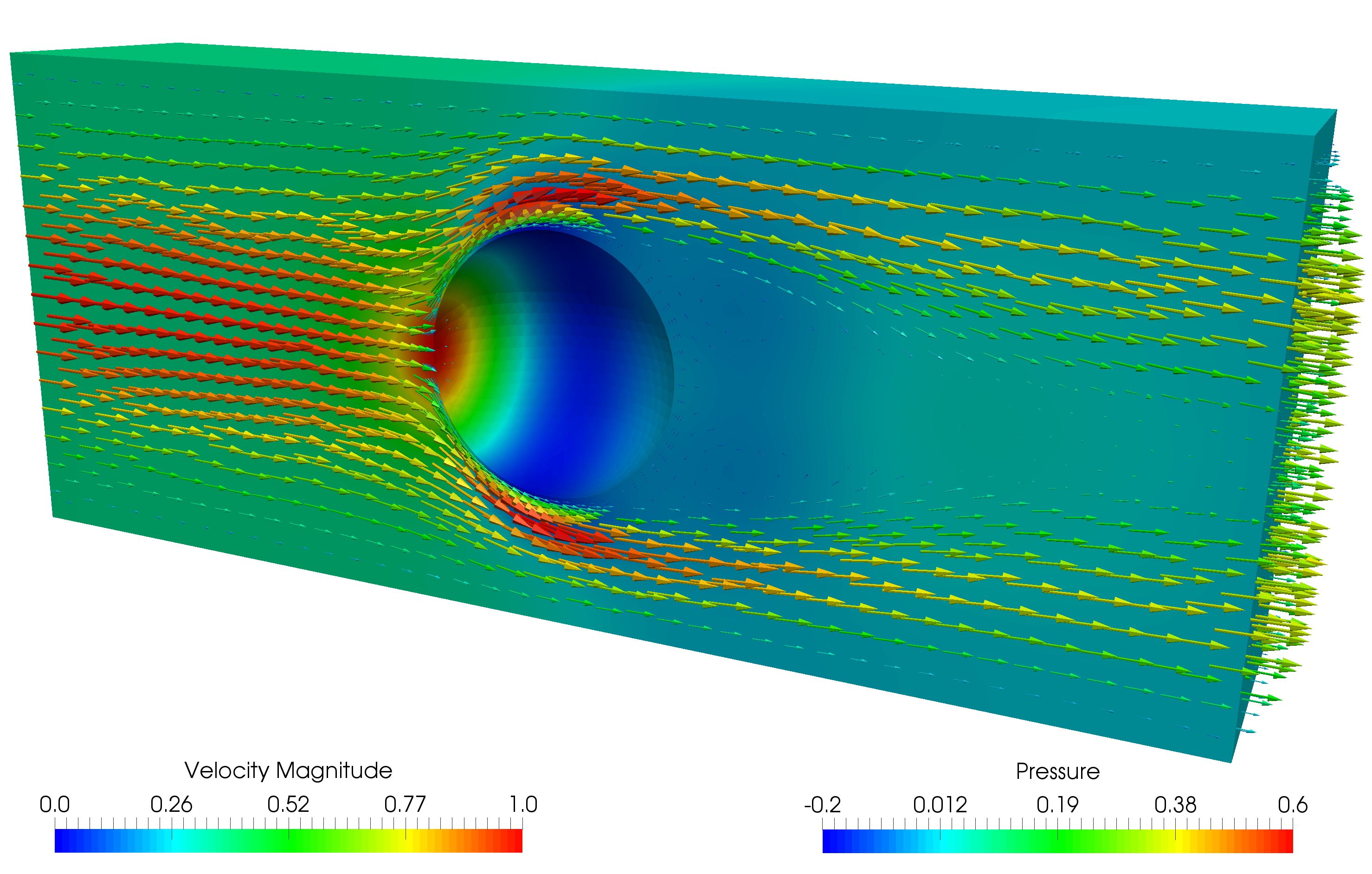
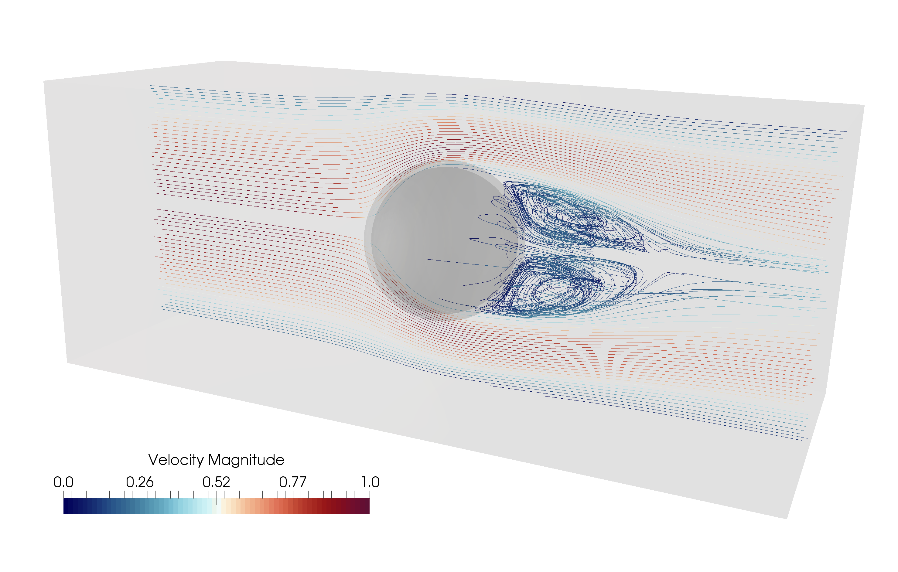
A contour plot of the centerline velocity magnitude and the corresponding (unscaled) velocity vector field at steady state is shown in Fig. 15(b). In this view, the cone-shaped recirculation region behind the sphere is visible, as is the rough location of the boundary layer separation point on the back half of the sphere. The steady state velocity and pressure fields along the channel centerline are shown in Fig. 16(a). In this figure, the velocity vectors are colored and scaled by the velocity magnitude, so the region of slow-moving flow in the wake of the sphere is once again visible. Finally, in Fig. 16(b), streamtraces originating from a line source placed directly behind the sphere are shown. The streamtraces help to visualize the three-dimensional nature of the wake region, and the entrainment of particles from the surrounding flow.

(a) Details of the hybrid mesh surrounding the sphere.

(b) Contour plot of velocity magnitude and (unscaled) velocity vectors.

Figure 15: Plots showing (15(a)) details of the hybrid prismatic/tetrahedral mesh near the sphere, and (15(b)) contour plot of the centerline velocity magnitude combined with unscaled velocity vectors to indicate the direction of the flow field. The approximate location of the boundary layer separation point on the downstream side of the sphere is visible, as are the extent of the recirculation zones in the wake.

(a) Centerline pressure contour plot and velocity vectors colored by magnitude.

(b) Streamtraces showing entrainment behind the sphere.

Figure 16: Plots showing (16(a)) the steady state centerline pressure and velocity vectors colored by $|\vec{u}|$, and (16(b)) streamtraces originating from just downstream of the sphere and colored by the velocity magnitude. In (16(a)) the vector length is proportional to $|\vec{u}|$, so it is difficult to see the three-dimensional nature of the region of recirculating flow directly behind the sphere, but this region is clearly visible in (16(b)).

7 Conclusions and future work

The stabilized finite element formulation of the INS equations in the navier_stokes module of MOOSE is currently adequate for solving small to medium-sized problems over a wide range of Reynolds numbers, on non-trivial 2D and 3D geometries. The software implementation of the INS equations has been verified for a number of simple test problems, and is developed under a modern and open continuous integration workflow to help guarantee high software quality. The navier_stokes module is also easy to integrate (without writing additional code) with existing and new MOOSE-based application codes since it is distributed directly with the MOOSE framework itself: all that should be required is a simple change to the application Makefile.

There are still a number of challenges and opportunities for collaboration to improve the quality and effectiveness of the INS implementation in the navier_stokes module. These opportunities range from the relatively straightforward, such as implementing LSIC stabilization, investigating and developing non-conforming velocity, discontinuous pressure, and divergence-free finite element discretizations, and adding MOOSE Actions to simplify and streamline the input file writing experience, to more involved tasks like implementing a coupled, stabilized temperature convection-diffusion equation and Boussinesq approximation term, implementing and testing turbulence models, and adding support for simulating non-Newtonian fluids. The closely-related low Mach number equations [81] are also of theoretical and practical interest for cases where temperature variations in the fluid are expected to be large, and would be appropriate to include in the navier_stokes module.

The largest outstanding challenges primarily involve improving the basic field-split preconditioning capabilities which are already present in the navier_stokes module, but are not currently widely used due to their cost and the lack of a general and efficient procedure for approximating the action of the Schur complement matrix. In this context, we also note the important role of multigrid methods (both geometric and algebraic variants) in the quest for developing scalable algorithms. The field-split approach, combined with geometric multigrid preconditioners, is probably the most promising avenue for applying the navier_stokes module to larger and more realistic applications. These techniques require a tight coupling between the finite element discretization and linear algebra components of the code, and a deep understanding of the physics involved. We are confident that the navier_stokes module itself will provide a valuable and flexible test bed for researching such methods in the future.

References

- [1] D. R. Gaston, C. J. Permann, J. W. Peterson, A. E. Slaughter, D. Andrš, Y. Wang, M. P. Short, D. M. Perez, M. R. Tonks, J. Ortensi, and R. C. Martineau, “Physics-based multiscale coupling for full core nuclear reactor simulation,” Annals of Nuclear Energy, Special Issue on Multi-Physics Modelling of LWR Static and Transient Behaviour, vol. 84, pp. 45–54, Oct. 2015. https://doi.org/10.1016/j.anucene.2014.09.060.
- [2] A. E. Slaughter, J. W. Peterson, D. R. Gaston, C. J. Permann, D. Andrš, and J. M. Miller, “Continuous integration for concurrent MOOSE framework and application development on GitHub,” Journal of Open Research Software, vol. 3, p. e14 (7 pages), Nov. 2015. https://doi.org/10.5334/jors.bx.
- [3] B. S. Kirk, J. W. Peterson, R. H. Stogner, and G. F. Carey, “libMesh: A C++ library for parallel adaptive mesh refinement/coarsening simulations,” Engineering with Computers, vol. 22, pp. 237–254, Dec. 2006. https://doi.org/10.1007/s00366-006-0049-3.
- [4] S. Balay, S. Abhyankar, M. F. Adams, J. Brown, P. Brune, K. Buschelman, L. Dalcin, V. Eijkhout, W. D. Gropp, D. Kaushik, M. G. Knepley, L. C. McInnes, K. Rupp, B. F. Smith, S. Zampini, H. Zhang, and H. Zhang, “PETSc Users Manual,” Tech. Rep. ANL-95/11 - Revision 3.7, Argonne National Laboratory, 2016. http://www.mcs.anl.gov/petsc.
- [5] S. M. Allen and J. W. Cahn, “Ground state structures in ordered binary alloys with second neighbor interactions,” Acta Metallurgica, vol. 20, pp. 423–433, Mar. 1972. https://doi.org/10.1016/0001-6160(72)90037-5.
- [6] J. W. Cahn and J. E. Hilliard, “Free energy of a nonuniform system: I. Interfacial free energy,” Journal of Chemical Physics, vol. 28, pp. 258–267, Feb. 1958. https://doi.org/10.1063/1.1744102.
- [7] L. Zhang, M. R. Tonks, D. Gaston, J. W. Peterson, D. Andrs, P. C. Millett, and B. S. Biner, “A quantitative comparison between and elements for solving the Cahn–Hilliard equation,” Journal of Computational Physics, vol. 236, pp. 74–80, Mar. 2013. https://doi.org/10.1016/j.jcp.2012.12.001.
- [8] F. M. White, Viscous Fluid Flow. McGraw-Hill, 2nd ed., 1991.
- [9] F. M. White, Fluid Mechanics. McGraw-Hill, 7th ed., 2010.
- [10] R. L. Panton, Incompressible Flow. John Wiley and Sons, 4th ed., 2012.
- [11] B. R. Munson, A. P. Rothmayer, T. H. Okiishi, and W. W. Huebsch, Fundamentals of Fluid Mechanics. John Wiley and Sons, 7th ed., 1998.
- [12] G. F. Carey and J. T. Oden, Finite elements: Fluid mechanics, vol. 6. Prentice Hall, 1986.
- [13] R. H. Gallagher, R. Glowinski, P. M. Gresho, J. T. Oden, and O. C. Zienkiewicz, Finite Elements in Fluids, vol. 7. Wiley-Interscience and New York, 1988.
- [14] P. M. Gresho and R. L. Sani, Incompressible flow and the finite element method. Volume 1: Advection-diffusion. John Wiley and Sons, 1998.
- [15] P. M. Gresho and R. L. Sani, Incompressible flow and the finite element method. Volume 2: Isothermal laminar flow. John Wiley and Sons, 2002.
- [16] R. W. Lewis, P. Nithiarasu, and K. N. Seetharamu, Fundamentals of the finite element method for heat and fluid flow. Wiley, 2004.
- [17] O. C. Zienkiewicz, R. L. Taylor, and P. Nithiarasu, The finite element method for fluid dynamics. Elsevier, 6th ed., 2005.
- [18] C. Taylor, J. Rance, and J. O. Medwell, “A note on the imposition of traction boundary conditions when using the FEM for solving incompressible flow problems,” Communications in Applied Numerical Methods, vol. 1, pp. 113–121, May 1985. https://doi.org/10.1002/cnm.1630010305.
- [19] M. Gad-el-Hak, “Stokes’ hypothesis for a Newtonian, isotropic fluid,” Journal of Fluids Engineering, vol. 117, pp. 3–5, Mar. 1995. https://doi.org/10.1115/1.2816816.
- [20] T. A. Zang, “On the rotation and skew-symmetric forms for incompressible flow simulations,” Applied Numerical Mathematics, vol. 7, pp. 27–40, Jan. 1991. https://doi.org/10.1016/0168-9274(91)90102-6.
- [21] P. Bochev and R. B. Lehoucq, “On the finite element solution of the pure Neumann problem,” SIAM Review, vol. 47, no. 1, pp. 50–66, 2005. https://doi.org/10.1137/S0036144503426074.
- [22] P. E. Gill, W. Murray, D. B. Ponceleon, and M. A. Saunders, “Preconditioners for indefinite systems arising in optimization,” SIAM Journal on Matrix Analysis and Applications, vol. 13, no. 1, pp. 292–311, 1992. https://doi.org/10.1137/0613022.
- [23] M. F. Murphy, G. H. Golub, and A. J. Wathen, “A note on preconditioning for indefinite linear systems,” SIAM Journal on Scientific Computing, vol. 21, no. 6, pp. 1969–1972, 2000. https://doi.org/10.1137/S1064827599355153.
- [24] D. F. Griffiths, “The ‘No Boundary Condition’ outflow boundary condition,” International Journal for Numerical Methods in Fluids, vol. 24, pp. 393–411, Feb. 1997. http://tinyurl.com/y77au2k3.
- [25] M. A. Olshanskii, “A low order Galerkin finite element method for the Navier–Stokes equations of steady incompressible flow: A stabilization issue and iterative methods,” Computer Methods in Applied Mechanics and Engineering, vol. 191, pp. 5515–5536, Nov. 2002. https://doi.org/10.1016/S0045-7825(02)00513-3.
- [26] O. A. Ladyzhenskaya, The mathematical theory of viscous incompressible flow. PO Box 786, Cooper Station, New York, New York 10276: Gordon and Breach Science Publishers, 1969. 2nd edition of the English translation by R. A. Silverman, vol. 2 of the series “Mathematics and its Applications”.
- [27] I. Babuška, “The finite element method with Lagrange multipliers,” Numerische Mathematik, vol. 20, pp. 179–192, June 1973. https://doi.org/10.1007/BF01436561.
- [28] F. Brezzi, “On the existence, uniqueness and approximation of saddle-point problems arising from Lagrangian multipliers,” ESAIM: Mathematical Modelling and Numerical Analysis – Modélisation Mathématique et Analyse Numérique, vol. 8, no. R2, pp. 129–151, 1974. http://tinyurl.com/y9d3v33h.
- [29] J. Donea and A. Huerta, Finite Element Methods for Flow Problems. John Wiley and Sons, 2003.
- [30] F. Brezzi, M. O. Bristeau, L. P. Franca, M. Mallet, and G. Rogé, “A relationship between stabilized finite element methods and the Galerkin method with bubble functions,” Computer Methods in Applied Mechanics and Engineering, vol. 96, pp. 117–129, Apr. 1992. https://doi.org/10.1016/0045-7825(92)90102-P.
- [31] T. J. R. Hughes, “Multiscale phenomena: Green’s functions, the Dirichlet-to-Neumann formulation, subgrid scale models, bubbles, and the origins of stabilized methods,” Computer Methods in Applied Mechanics and Engineering, vol. 127, pp. 387–401, Nov. 1995. https://doi.org/10.1016/0045-7825(95)00844-9.
- [32] F. Brezzi, L. P. Franca, T. J. R. Hughes, and A. Russo, “,” Computer Methods in Applied Mechanics and Engineering, vol. 145, pp. 329–339, June 1997. https://doi.org/10.1016/S0045-7825(96)01221-2.
- [33] R. Codina, “Stabilization of incompressibility and convection through orthogonal sub-scales in finite element methods,” Computer Methods in Applied Mechanics and Engineering, vol. 190, pp. 1579–1599, Dec. 2000. https://doi.org/10.1016/S0045-7825(00)00254-1.
- [34] L. P. Franca, A. L. Madureira, and F. Valentin, “Towards multiscale functions: Enriching finite element spaces with local but not bubble-like functions,” Computer Methods in Applied Mechanics and Engineering, vol. 194, pp. 3006–3021, July 2005. https://doi.org/10.1016/j.cma.2004.07.029.
- [35] A. N. Brooks and T. J. R. Hughes, “Streamline upwind/Petrov–Galerkin formulations for convection dominated flows with particular emphasis on the incompressible Navier–Stokes equations,” Computer Methods in Applied Mechanics and Engineering, vol. 32, pp. 199–259, Sept. 1982. https://doi.org/10.1016/0045-7825(82)90071-8.
- [36] C. Johnson and J. Saranen, “Streamline diffusion methods for the incompressible Euler and Navier–Stokes equations,” Mathematics of Computation, vol. 47, pp. 1–18, July 1986. https://doi.org/10.1090/S0025-5718-1986-0842120-4.
- [37] F. Shakib, T. J. R. Hughes, and Z. Johan, “A new finite element formulation for computational fluid dynamics: X. The compressible Euler and Navier–Stokes equations,” Computer Methods in Applied Mechanics and Engineering, vol. 89, pp. 141–219, Aug. 1991. https://doi.org/10.1016/0045-7825(91)90041-4.
- [38] T. E. Tezduyar, “Stabilized finite element formulations for incompressible flow computations,” Advances in Applied Mechanics, vol. 28, pp. 1–44, 1991. https://doi.org/10.1016/S0065-2156(08)70153-4.
- [39] L. P. Franca and S. L. Frey, “Stabilized finite element methods: II. The incompressible Navier–Stokes equations,” Computer Methods in Applied Mechanics and Engineering, vol. 99, pp. 209–233, Sept. 1992. https://doi.org/10.1016/0045-7825(92)90041-H.
- [40] L. P. Franca and T. J. R. Hughes, “Convergence analyses of Galerkin least-squares methods for symmetric advective-diffusive forms of the Stokes and incompressible Navier–Stokes equations,” Computer Methods in Applied Mechanics and Engineering, vol. 105, pp. 285–298, June 1993. https://doi.org/10.1016/0045-7825(93)90126-I.
- [41] T. E. Tezduyar and Y. Osawa, “Finite element stabilization parameters computed from element matrices and vectors,” Computer Methods in Applied Mechanics and Engineering, vol. 190, pp. 411–430, Oct. 2000. https://doi.org/10.1016/S0045-7825(00)00211-5.
- [42] R. Codina, E. Oñate, and M. Cervera, “The intrinsic time for the Streamline Upwind/Petrov–Galerkin formulation using quadratic elements,” Computer Methods in Applied Mechanics and Engineering, vol. 94, pp. 239–262, Jan. 1992. https://doi.org/10.1016/0045-7825(92)90149-E.
- [43] T. J. R. Hughes, L. P. Franca, and M. Balestra, “A new finite element formulation for computational fluid dynamics: V. Circumventing the Babuška–Brezzi condition: A stable Petrov–Galerkin formulation of the Stokes problem accommodating equal-order interpolations,” Computer Methods in Applied Mechanics and Engineering, vol. 59, pp. 85–99, Nov. 1986. https://doi.org/10.1016/0045-7825(86)90025-3.
- [44] T. J. R. Hughes and L. P. Franca, “A new finite element formulation for computational fluid dynamics: VII. The Stokes problem with various well-posed boundary conditions: Symmetric formulations that converge for all velocity/pressure spaces,” Computer Methods in Applied Mechanics and Engineering, vol. 65, pp. 85–96, Nov. 1987. https://doi.org/10.1016/0045-7825(87)90184-8.
- [45] J. Douglas and J. Wang, “An absolutely stabilized finite element method for the Stokes problem,” Mathematics of Computation, vol. 52, pp. 495–508, Apr. 1989. https://doi.org/10.1090/S0025-5718-1989-0958871-X.
- [46] P. Hansbo and A. Szepessy, “A velocity-pressure streamline diffusion method for the incompressible Navier–Stokes equations,” Computer Methods in Applied Mechanics and Engineering, vol. 84, pp. 175–192, Dec. 1990. https://doi.org/10.1016/0045-7825(90)90116-4.
- [47] T. E. Tezduyar, S. Mittal, S. E. Ray, and R. Shih, “Incompressible flow computations with stabilized bilinear and linear equal-order-interpolation velocity-pressure elements,” Computer Methods in Applied Mechanics and Engineering, vol. 95, pp. 221–242, Mar. 1992. https://doi.org/10.1016/0045-7825(92)90141-6.
- [48] R. Codina and O. Soto, “Finite element solution of the Stokes problem with dominating Coriolis force,” Computer Methods in Applied Mechanics and Engineering, vol. 142, pp. 215–234, Mar. 1997. https://doi.org/10.1016/S0045-7825(96)01141-3.
- [49] R. Codina, “A stabilized finite element method for generalized stationary incompressible flows,” Computer Methods in Applied Mechanics and Engineering, vol. 190, pp. 2681–2706, Feb. 2001. https://doi.org/10.1016/S0045-7825(00)00260-7.
- [50] T. Gelhard, G. Lube, M. A. Olshanskii, and J.-H. Starcke, “Stabilized finite element schemes with LBB-stable elements for incompressible flows,” Journal of Computational and Applied Mathematics, vol. 177, pp. 243–267, May 2005. https://doi.org/10.1016/j.cam.2004.09.017.
- [51] A. Iserles, A First Course in the Numerical Analysis of Differential Equations. Cambridge University Press, 2nd ed., 2009.
- [52] R. S. Dembo, S. C. Eisenstat, and T. Steihaug, “Inexact Newton Methods,” SIAM Journal on Numerical Analysis, vol. 19, no. 2, pp. 400–408, 1982. https://doi.org/10.1137/0719025.
- [53] Y. Saad, Iterative Methods for Sparse Linear Systems. SIAM, 2003.
- [54] P. N. Brown and Y. Saad, “Hybrid Krylov methods for nonlinear systems of equations,” SIAM Journal on Scientific and Statistical Computing, vol. 11, no. 3, pp. 450–481, 1990. https://doi.org/10.1137/0911026.
- [55] Y. Saad and M. H. Schultz, “GMRES: A generalized minimal residual algorithm for solving nonsymmetric linear systems,” SIAM Journal on Scientific and Statistical Computing, vol. 7, no. 3, pp. 856–869, 1986. https://doi.org/10.1137/0907058.
- [56] J. Nocedal and S. J. Wright, Numerical Optimization. Springer, 2006.
- [57] M. Pernice and H. F. Walker, “NITSOL: A Newton iterative solver for nonlinear systems,” SIAM Journal on Scientific Computing, vol. 19, no. 1, pp. 302–318, 1998. https://doi.org/10.1137/S1064827596303843.
- [58] B. F. Smith, P. E. Bjørstad, and W. D. Gropp, Domain Decomposition: Parallel Multilevel Methods for Elliptic Partial Differential Equations. Cambridge University Press, 2004.
- [59] F. Kong and X.-C. Cai, “Scalability study of an implicit solver for coupled fluid-structure interaction problems on unstructured meshes in 3D,” The International Journal of High Performance Computing Applications, pp. 1–13, May 2016. https://doi.org/10.1177/1094342016646437.
- [60] F. Kong and X.-C. Cai, “A scalable nonlinear fluid-structure interaction solver based on a Schwarz preconditioner with isogeometric unstructured coarse spaces in 3D,” Journal of Computational Physics, vol. 340, pp. 498–518, July 2017. https://doi.org/10.1016/j.jcp.2017.03.043.
- [61] H. Elman, V. E. Howle, J. Shadid, R. Shuttleworth, and R. Tuminaro, “A taxonomy and comparison of parallel block multi-level preconditioners for the incompressible Navier–Stokes equations,” Journal of Computational Physics, vol. 227, pp. 1790–1808, Jan. 2008. https://doi.org/10.1016/j.jcp.2007.09.026.
- [62] A. Quarteroni, F. Saleri, and A. Veneziani, “Factorization methods for the numerical approximation of Navier–Stokes equations,” Computer Methods in Applied Mechanics and Engineering, vol. 188, pp. 505–526, July 2000. https://doi.org/10.1016/S0045-7825(99)00192-9.
- [63] P. Wesseling, Principles of Computational Fluid Dynamics. Springer–Verlag New York, Inc., 2009.
- [64] W. Bangerth, R. Hartmann, and G. Kanschat, “deal.II—–A general-purpose object-oriented finite element library,” ACM Transactions on Mathematical Software (TOMS), vol. 33, no. 4, p. 24 (27 pages), 2007. https://doi.org/10.1145/1268776.1268779.
- [65] P. Bastian, M. Blatt, A. Dedner, C. Engwer, R. Klöfkorn, R. Kornhuber, M. Ohlberger, and O. Sander, “A generic grid interface for parallel and adaptive scientific computing. Part II: Implementation and tests in DUNE,” Computing, vol. 82, pp. 121–138, July 2008. https://doi.org/10.1007/s00607-008-0004-9.
- [66] P. T. Bauman and R. H. Stogner, “GRINS: A multiphysics framework based on the libMesh finite element library,” SIAM Journal on Scientific Computing, vol. 38, no. 5, pp. S78–S100, 2016. https://doi.org/10.1137/15M1026110.
- [67] F. Hecht, “New development in FreeFem++,” Journal of Numerical Mathematics, vol. 20, no. 3–4, pp. 251–265, 2012. https://doi.org/10.1515/jnum-2012-0013.
- [68] H. Jasak, A. Jemcov, and Ž. Tuković, “OpenFOAM: A C++ library for complex physics simulations,” in Proceedings of the International Workshop on Coupled Methods in Numerical Dynamics (CMND 2007), (Dubrovnik, Croatia), Sept. 19–21, 2007. http://tinyurl.com/ybvnk7e5.
- [69] A. Logg, K.-A. Mardal, and G. Wells, “Automated solution of differential equations by the finite element method: The FEniCS book,” in Lecture Notes in Computational Science and Engineering, vol. 84, Springer Science & Business Media, 2012. http://tinyurl.com/y9pml5tx.
- [70] A. Henderson, J. Ahrens, C. Law, et al., The ParaView Guide. Clifton Park, NY: Kitware, 2004.
- [71] P. J. Roache, Verification and validation in computational science and engineering. Albuquerque, NM: Hermosa, 1998.
- [72] C. Johnson, U. Nävert, and J. Pitkäranta, “Finite element methods for linear hyperbolic problems,” Computer Methods in Applied Mechanics and Engineering, vol. 45, pp. 285–312, Sept. 1984. https://doi.org/10.1016/0045-7825(84)90158-0.
- [73] T. J. R. Hughes and M. Mallet, “A new finite element formulation for computational fluid dynamics: II. Beyond SUPG,” Computer Methods in Applied Mechanics and Engineering, vol. 54, pp. 341–355, Mar. 1986. https://doi.org/10.1016/0045-7825(86)90110-6.
- [74] G. B. Jeffery, “The two-dimensional steady motion of a viscous fluid,” Philosophical Magazine Series 6, vol. 29, no. 172, pp. 455–465, 1915. https://doi.org/10.1080/14786440408635327.
- [75] G. Hamel, “Spiralförmige Bewegungen zäher Flüssigkeiten,” Jahresbericht der Deutschen Mathematiker Vereinigung, vol. 25, pp. 34–60, 1916.
- [76] L. Rosenhead, “The steady two-dimensional radial flow of viscous fluid between two inclined plane walls,” Proceedings of the Royal Society of London A: Mathematical, Physical and Engineering Sciences, vol. 175, no. 963, pp. 436–467, 1940. https://doi.org/10.1098/rspa.1940.0068.
- [77] P. Haines, R. E. Hewitt, and A. L. Hazel, “The Jeffery–Hamel similarity solution and its relation to flow in a diverging channel,” Journal of Fluid Mechanics, vol. 687, pp. 404–430, Nov. 2011. https://doi.org/10.1017/jfm.2011.362.
- [78] J. W. Peterson and R. H. Stogner, “A -continuous finite element formulation for solving the Jeffery-Hamel boundary value problem.” ArXiv e-print, Dec. 2016. http://arxiv.org/abs/1612.06312.
- [79] P. M. Gresho, D. K. Gartling, J. R. Torczynski, K. A. Cliffe, K. H. Winters, T. J. Garratt, A. Spence, and J. W. Goodrich, “Is the steady viscous incompressible two-dimensional flow over a backward-facing step at stable?,” International Journal for Numerical Methods in Fluids, vol. 17, pp. 501–541, Sept. 1993. https://doi.org/10.1002/fld.1650170605.
- [80] X. S. Li and J. W. Demmel, “SuperLU_DIST: A scalable distributed-memory sparse direct solver for unsymmetric linear systems,” ACM Transactions on Mathematical Software, vol. 29, pp. 110–140, June 2003. https://doi.org/10.1145/779359.779361.
- [81] R. G. Rehm and H. R. Baum, “The equations of motion for thermally driven, buoyant flows,” Journal of Research of the National Bureau of Standards, vol. 83, no. 3, pp. 297–308, 1978. http://tinyurl.com/y87hovk4.