Avoiding Communication in Proximal Methods for Convex Optimization Problems

Abstract

The fast iterative soft thresholding algorithm (FISTA) is used to solve convex regularized optimization problems in machine learning. Distributed implementations of the algorithm have become popular since they enable the analysis of large datasets. However, existing formulations of FISTA communicate data at every iteration which reduces its performance on modern distributed architectures. The communication costs of FISTA, including bandwidth and latency costs, is closely tied to the mathematical formulation of the algorithm. This work reformulates FISTA to communicate data at every “k” iterations and reduce data communication when operating on large data sets. We formulate the algorithm for two different optimization methods on the Lasso problem and show that the latency cost is reduced by a factor of k while bandwidth and floating-point operation costs remain the same. The convergence rates and stability properties of the reformulated algorithms are similar to the standard formulations. The performance of communication-avoiding FISTA and Proximal Newton methods is evaluated on 1 to 1024 nodes for multiple benchmarks and demonstrate average speedups of 3-10$\times$ with scaling properties that outperform the classical algorithms.

I Introduction

Mathematical optimization is one of the main pillars of machine learning, where parameter values are computed based on observed data. Applications in many big data and large-scale scientific computing domains need the solution to convex optimization problems [1]. The performance of these optimization problems is often dominated by communication which is closely tied to the formulation of the algorithms. A popular approach to estimate parameters in convex optimization problems is solving a regularized least square problem that can solve many ill-conditioned systems. L1-regularized least square problems are often solved using the class of proximal methods, called iterative shrinkage-thresholding algorithms (ISTA) [2]. The advantage of ISTA is in its simplicity. However, ISTA has also been recognized as a slow method in terms of convergence rate [3]. It is well known that for large-scale problems first order methods are often the only practical option. Fast iterative shrinkage-thresholding algorithm (FISTA) extends ISTA while preserving the computational simplicity of ISTA and has a global rate of convergence that is significantly better, both theoretically and practically [3]. Another class of widely used proximal methods are proximal Newton-type methods (PNM) that use second order information in their proximal mapping which have a superlinear rate of convergence [4]. Stochastic formulations of FISTA and PNM, abbreviated as SFISTA and SPNM, are often more efficient for processing large data [1] and thus are used as the base algorithms in this work. These methods are iterative by nature, therefore need to communicate data in each iteration. Since communication is more expensive than arithmetic, the scalability and performance of these algorithms are bound by communication costs on distributed architectures.

The performance of an algorithm on modern computing architectures depends on the costs of arithmetic and data communication between different levels of memory and processors over a network. The communication cost of an algorithm is computed by adding bandwidth costs, the time required to move words, and latency costs, the time to communicate messages between processors. On modern computer architectures the cost of communication is often orders of magnitude larger than floating point operation costs and this gap is increasing [5]. Classical formulations of optimization methods are inherently communication-bound. Therefore, to achieve high-performance on modern distributed platforms, optimization methods have to be reformulated to minimize communication and data movement rather than arithmetic complexity [6].

Recent work has developed algorithms to reduce communication in a number of optimization and machine learning methods. Communication efficient optimization libraries such as [7, 8, 9] attempt to reduce communication, though they may change the convergence behavior of the algorithm. For example, CoCoA [7] uses a local solver on each machine and shares information between the solvers with highly flexible communication schemes. HOGWILD! [8] implements stochastic gradient descent (SGD) without locking which achieves a nearly optimal convergence rate (compared to its serial counterpart) only if the optimization problem is sparse. K-AVG [9] modifies SGD by communicating every k iterations. This method changes the convergence behavior of SGD by arguing that frequent synchronization does not always lead to faster convergence. You et. al. [10] present a partitioning algorithm to efficiently divide the training set among processors for support vector machines (SVMs). Their approach works well for SVMs but does not extend to optimization problems in general. P-packSVM [11] uses a similar approach to ours to derive an SGD-based SVM algorithm which communicates every k iterations. Our work extends this technique to proximal least-squares problems solved by FISTA and Newton-type methods.

Standard optimization algorithms are iterative and compute an update direction per iteration by communicating data. Krylov iterative solvers, frequently used to solve linear systems of equations, follow a similar pattern. Efforts to reformulate standard formulations of Krylov solvers by scientific computing practitioners has lead the developed of k-step Krylov solvers [12, 13]. These algorithms compute k basis vectors at-once by unrolling k iterations of the standard algorithm.With careful partitioning of the original data matrix [14, 15], the matrix powers kernel in the reformulated Krylov methods can be optimized to reduce communication costs by O(k) compared to the classical algorithm. k-step methods are powerful as they are arithmetically the same as the standard methods and thus often preserve convergence properties. However, data partitioning costs can be very high in the communication-avoiding implementations of k-step Krylov methods and matrices from many optimization problems are not good candidates for such partitioning. Devarakonda et. al. extend k-step methods to the block coordinate decent (BCD) methods [16]. Their implementation reduces latency costs by a factor k while increasing the bandwidth and floating point operations (flops) costs.

In this work we introduce k-step formulations for the stochastic FISTA (SFISTA) and stochastic proximal Newton-type method (SPNM) algorithms. Unlike the k-step formulations of Krylov methods which avoid communication by partitioning data—such an approach does not work for large matrices in optimization problems—we use randomized sampling to reformulate the classical algorithms and to reduce communication. Randomization enables us to control the communication and computation cost in the reformulated algorithm. Our approach reduces the latency cost without significantly increasing bandwidth costs or flops.

We introduce communication-avoiding implementations of SFISTA (CA-SFISTA) and SPNM (CA-SPNM) to reduce communication by reducing latency costs. Figure 1 shows the execution time of SFISTA for the covtype dataset. SFISTA shows poor scaling properties when the number of processors increase and demonstrates no performance gains on 64 processors vs. one processor. CA-SFISTA can solve the regularized least square problem by iteratively updating the optimization variable every k iterations and reduces the latency cost by a factor of k. CA-SFISTA and CA-SPNM outperform the classical algorithms without changing the convergence behavior. We control randomization by sampling from the distributed data between processors. Random sampling enables us to create sub-samples of data to improve locality and arithmetic costs in each iteration. Unrolling of iterations to reformulate the standard algorithms is also made possible through random sampling.

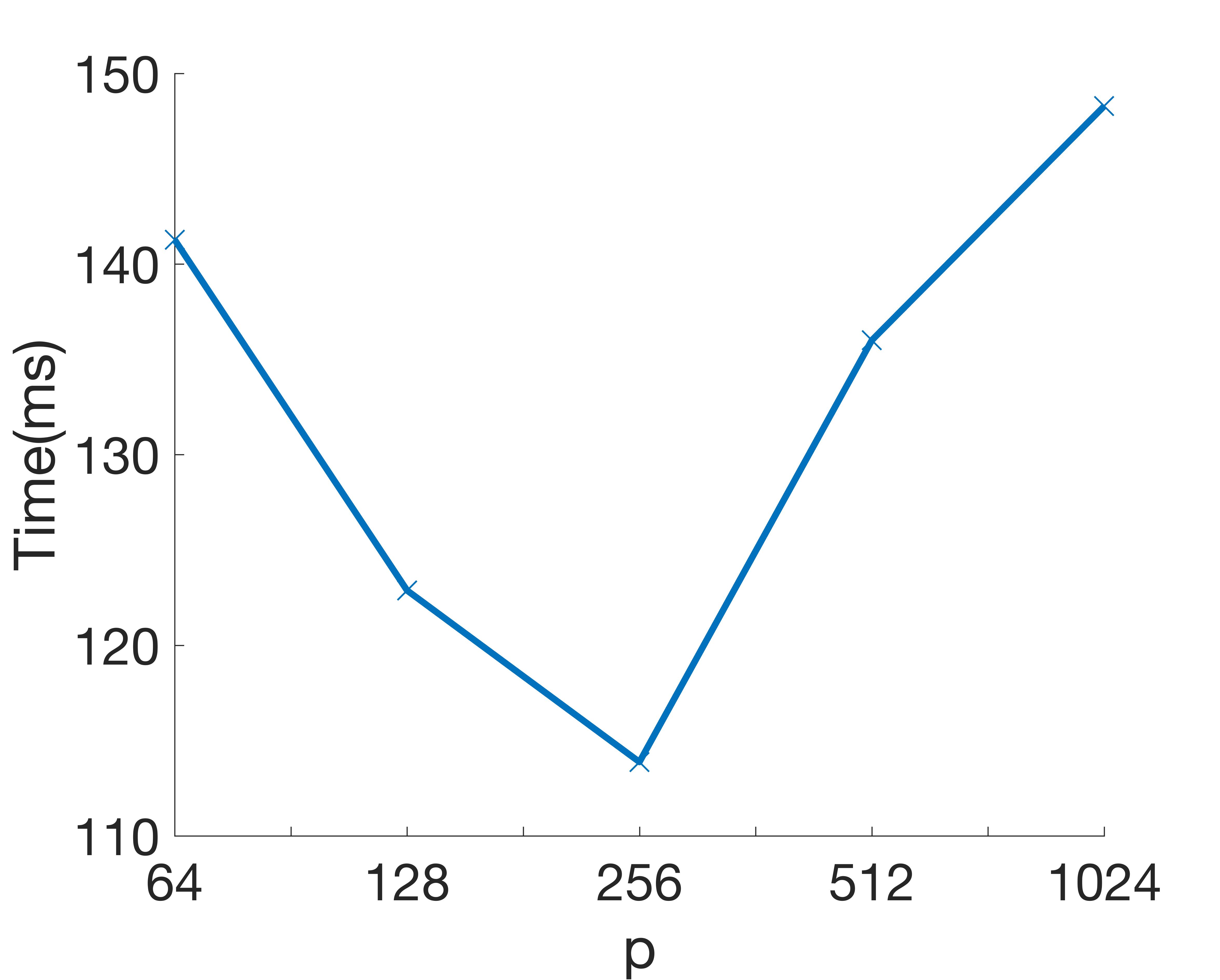
Figure 1: Execution time of SFISTA for the covtype dataset.

The following summarizes the contributions of the work:

• We introduce CA-SFISTA and CA-SPNM that provably reduce the latency cost of two well-known optimization methods used to solve L1-regularized least square problems by a factor of $O(k)$ without changing the convergence behavior of the original algorithms.

• The communication-avoiding algorithms achieve upto 10X speedup on the target supercomputers.

• We develop a randomized sampling strategy that creates samples of data for each processor to facilitate the derivation and implementations of CA-SFISTA and CA-SPNM.

• Computation and communication costs of the classical algorithms as well as the proposed communication-avoiding algorithms are presented. Our analysis shows that CA-SPNM and CA-SFISTA reduce communication costs without changing the floating points operation or bandwidth costs.

II Background

This section introduces the L1-regularized least squares problems and algorithmic approaches for their solution. Details of the communication model used throughout the paper is also provided.

II-A Regularized Least Squares Problem

Consider the following composite additive cost optimization problem of the form

$$\operatornamewithlimits{min}\limits_{w\in\mathbb{R}^{d}}\;{F(w)\equiv f(w)+g(w)}$$ (1)

where $g:\mathbb{R}^{d}\to\mathbb{R}$ is a continuous, convex, possibly nonsmooth function and $f:\mathbb{R}^{d}\to\mathbb{R}$ is a smooth and convex function, with a Lipschitz-continuous gradient. Let $L(f)$ be the Lipschitz constant of the gradient of $f$. This form can represent a large class of regression problems based on different choices of $f$ and $g$. In particular, the L1-regularized least squares problem, a.k.a. the least absolute shrinkage and selection operator (LASSO) problem, is a special case where

$$f(w)=\frac{1}{2n}\|X^{T}w-y\|_{2}^{2},\quad g(w)=\lambda\|w\|_{1},$$

when $X\in\mathbb{R}^{d\times n}$ is the input data matrix, where rows are the features and columns are the samples, $y\in\mathbb{R}^{n}$ holds the labels (or observations), $w\in\mathbb{R}^{d}$ is the optimization variable, and $\lambda\in\mathbb{R}$ is the regularization (penalty) parameter. The parameter $\lambda$ controls the sparsity of the solution, since increasing its value magnifies the effect of the second term $g(w)$, which itself is minimized at $w=0$. In this case, the gradient of $f(w)$ is given by:

$$\nabla f(w)=\frac{1}{n}(XX^{T}w-Xy).\$$ (2)

LASSO problems appear frequently in machine learning applications [17] including learning directed and undirected graphical models [18], online dictionary learning [19], elastic-net regularized problems [20], and feature selection in classification problems and data analysis [21, 22]. Let

$$\hat{w}=\operatornamewithlimits{argmin}\limits_{w}\frac{1}{2n}\|X^{T}w-y\|^{2}+\lambda\|w\|_{1}$$ (3)

be the optimal solution to the LASSO problem. The LASSO objective contains two parts, a quadratic penalty $f$ and the L1-regularization term $g$. Therefore, LASSO has regression characteristics by minimizing a least squares error and has subset selection features by shrinking the optimization variable and setting parts of it to zero.

II-B Solving LASSO

Among the most efficient methods for solving convex optimization problems of the form (1) are first order methods that use a proximal step in order to handle the possibly non-smooth part $g$. In particular, for the LASSO problem, the class of iterative soft thresholding algorithms, recently improved to FISTA [3], have become very popular due to their excellent performance. Each iteration of FISTA, involves computing a gradient followed by a soft thresholding operator. More recently, inspired by first order methods, proximal Newton methods have been introduced that use second order information (hessian) in their proximal part. These methods are globally convergent and could achieve a superlinear rate of convergence in the neighborhood of the optimal solution [4]. The fact that FISTA and proximal Newton methods are key algorithms for solving composite convex optimization problems motivates us to introduce communication-avoiding variants of these methods and discuss their computation and communication complexity.

II-C Communication Model

The cost of an algorithm includes arithmetic and computation. Traditionally, algorithms have been analyzed with floating point operation costs. However, communication costs are a crucial part in analyzing algorithms in large-scale simulations [23]. The cost of floating point operations and communication, including bandwidth and latency, can be combined to obtain the following model:

$$T=\gamma F+\alpha L+\beta W$$ (4)

where $T$ is the overall execution time approximated by a linear function of F, L, and W, which are total number of floating point operations, the number of messages sent, and the number of words moved respectively. Also, $\gamma$, $\alpha$, and $\beta$ are machine-specific parameters that show the cost of one floating point operation, the cost of sending a message, and the cost of moving a word. Among different communication models, the LogP [24] and LogGP [25] models are often used to develop communication models for parallel architectures. The communication model used in this paper is a simplified model known as $\alpha-\beta$ which uses $\gamma$, $\alpha$, and $\beta$ and shows the effect of communication and computation on the algorithm cost.

III Classical Stochastic algorithms

Even though there are some advantages to using batch optimization methods, multiple intuitive, practical, and theoretical reasons exist for using stochastic optimization methods. Stochastic methods can use information more efficiently than batch methods by choosing data randomly from the data matrix. In particular, for large-scale machine learning problems, training sets involve a good deal of (approximate) redundant data which makes batch methods inefficient in-practice. Theoretical analysis also favors stochastic methods for many big data scenarios [1]. This section explains the SFISTA and SPNM algorithms and analyzes their computation and communication costs. The associated costs are derived under the assumption that columns of $X$ are distributed in a way that each processor has roughly the same number of non-zeros. The vector $y$ is distributed among processors while vectors with dimension $d$ such as $v$ and $w$ are replicated on all processors. Finally, we assume that $n\gg d$ which means we are dealing with many observations in the application.

III-A Stochastic Fast Iterative Shrinkage-Thresholding Algorithm (SFISTA)

Computing the gradient in (2) is very expensive since the data matrix $X$ is being multiplied by its transpose. The cost of this operation can be reduced by sampling from the original matrix, leading to a randomized variant of FISTA [26, 27]. If $b$ percent of columns of $X$ are sampled, the new gradient vector is obtained by:

$$\nabla f(w)=\frac{1}{m}(XI_{j}I_{j}^{T}X^{T}w-XI_{j}I_{j}^{T}y)\$$ (5)

where $m=\lfloor bn\rfloor$ and $I_{j}$ is a random matrix containing one non-zero per column representing samples used for computing the gradient. Therefore the generalized gradient update is:

$$w_{j+1}=S_{\lambda t}(w_{j}-t_{j}\nabla f(w_{j}))$$ (6)

where $S_{\lambda}$ is the soft thresholding operator defined as:

$$S_{\lambda}(w)]_{i}=\begin{cases}w_{i}-\lambda&\text{if}\ w_{i}>\lambda\\ 0&\text{if}\ -\lambda\leq w_{i}\leq\lambda\\ w_{i}+\lambda&\text{if}\ w_{i}<-\lambda\par\end{cases}$$ (7)

where $[.]_{i}$ represents the i-th element of a vector. FISTA accelerates the rate of generalized gradient by modifying the update rule as follows:

$$w_{j+1}=S_{\lambda t}(v_{j}-t_{j}\nabla f(w_{j}))$$ (8)

where $v_{j}$ is the auxiliary variable defined as:

$$v_{j}=w_{j}+\frac{j-2}{j}\Delta w_{j}\$$ (9)

and $\Delta w_{j}=w_{j}-w_{j-1}$. Algorithm I shows the SFISTA algorithm for solving the LASSO problem.

III-B Stochastic Proximal Newton Methods (SPNM)

FISTA uses the first order information of $f$ (gradient) to update the optimization variable. However, proximal Newton methods solve the same problem with second order information (Hessian), or an approximation of it, to compute the smooth segment of the composite function (1). Proximal Newton methods achieve a superlinear convergence rate in the vicinity of the optimal solution [4]. As discussed in section II-A, since LASSO starts with an initial condition at $w=0$ and because the optimal solution is typically very sparse, the sequence of $w_{k}$ will be close enough to the optimal solution for different values of k. Therefore, very often proximal Newton methods achieve a superlinear convergence rate and converge faster than FISTA. Proximal Newton methods solve (1) with quadratic approximation to the smooth function $f$ in each iteration [4] as follows:

$$\begin{split}w_{j+1}&=\operatornamewithlimits{argmin}\limits_{y}\nabla f(w_{j})^{T}(y-w_{j})\\ &+\frac{1}{2}(y-w_{j})^{T}H_{j}(y-w_{j})+g(y)\end{split}$$ (10)

where $H_{j}$ is the approximation of the Hessian $f$ at iteration $j$. Since a closed form solution of (10) does not exist, a first order algorithm is often used to solve (10) and to update the optimization variable. Algorithm II shows the stochastic proximal Newton method for solving LASSO. As demonstrated, the SPNM algorithm takes a block of data, approximates the Hessian based on sampled columns, and uses a first order solver to solve (10) in lines 7-10 with $Q$ updates on the optimization variable. Thus, SPNM can be seen as a first order solver operating on blocks of data.

TABLE I: The SFISTA algorithm

1:	Input: $X\in\mathbb{R}^{d\times n}$, $y\in\mathbb{R}^{n}$, $w_{0}\in\mathbb{R}^{d}$, K$>$1 and $b\in\left(0,1\right]$.
2:	set $m=\lfloor bn\rfloor$
3:	for $j=0,1,...,T$ do
4:	Generate $I_{j}=[e_{i_{1}},e_{i_{2}},...,e_{i_{m}}]\in\mathbb{R}^{n\times m}$ where
	$\{i_{h}\in[d]|h=1,...,m\}$ is chosen uniformly at random
5:	$\nabla f(w_{j})=\frac{1}{m}XI_{j}I_{j}^{T}X^{T}w_{j-1}-\frac{1}{m}XI_{j}I_{j}^{T}y$
6:	$v_{j}=w_{j-1}+\frac{j-2}{j}(\Delta w_{j-1})$
7:	$w_{j}=S_{\lambda t_{j}}(v_{j}-t_{j}\nabla f(w_{j}))$
8:	output $w_{T}$

TABLE II: The SPNM algorithm

1:	Input: $X\in\mathbb{R}^{d\times n}$, $y\in\mathbb{R}^{n}$, $w_{0}\in\mathbb{R}^{d}$, K$>$1 and $b\in\left(0,1\right]$.
2:	set $m=\lfloor bn\rfloor$
3:	for $j=0,1,...,T$ do
4:	Generate $I_{j}=[e_{i_{1}},e_{i_{2}},...,e_{i_{m}}]\in\mathbb{R}^{n\times m}$ where
	$\{i_{h}\in[d]|h=1,...,m\}$ is chosen uniformly at random
5:	$\nabla f(w_{j})=\frac{1}{m}XI_{j}I_{j}^{T}X^{T}w_{j-1}-\frac{1}{m}XI_{j}I_{j}^{T}y$
6:	$z_{0}=w_{j-1}$
7:	for $q=1,...,Q$
8:	$z_{q}=S_{\lambda t_{k}}(z_{q-1}-t_{j}\nabla f(z_{q}))$
9:	$q=q+1$
10:	$w_{j}=z_{Q}$
11:	output $w_{T}$

The following theorems analyze the computation and communication costs of SFISTA and SPNM.

Theorem 1. $T$ iterations of SFISTA on $P$ processors over the critical path has following costs: F = $O(\frac{Td^{2}bn}{P})$ flops, W = $O(Td^{2}logP)$ words moved, L = $O(TlogP)$ messages and M = $O(\frac{dn}{P})$ words of memory.
Proof. SFISTA computes the gradient in line 5 which consists of three parts. The first part multiplies $X$ by its transpose in line 5 which requires $O(\frac{d^{2}bn}{P})$ operations and communicates $O(d^{2}logP)$ words and $O(logP)$ messages. Computing the second part which involves multiplying sampled $X$ and $y$, requires $O(\frac{dbn}{P})$ operations and needs $O(dlogP)$ words with $O(logP)$ messages. These two operations dominate other costs of the algorithm. Finally, the algorithm computes the gradient and updates the optimization variable redundantly on processors. Computing the gradient (line 5) requires $O(d^{2})$ operations without any communication between processors. The vector updates need $O(d)$ operations. Therefore, the total cost of SFISTA for $T$ iterations is $O(\frac{Td^{2}bn}{P})$ flops, $O(Td^{2}logP)$ words, and $O(TlogP)$ messages. Each processor needs enough memory to store three parts of $\nabla f$,$v_{j},w_{j}$ and $\frac{1}{P}$-th of $X$. Therefore, it needs $d^{2}+d+d+d+d+\frac{dn}{P}=O(\frac{dn}{P})$ words of memory.

Theorem 2. T iterations of SPNM on $P$ processors over the critical path has the following costs: F = $O(\frac{Td^{2}bn}{P}+\frac{Td^{2}}{\epsilon})$ flops, W = $O(Td^{2}logP)$ words moved, L = $O(TlogP)$ messages, and M = $O(\frac{dn}{P})$ words of memory.
Proof. SPNM solves the minimization problem using the Hessian. This requires $O(\frac{1}{\epsilon})$ inner iterations in order to reach an $\epsilon$-optimal solution. An analysis similar to theorem 1 can be used to prove this theorem.

The communication bottleneck of SFISTA and SPNM: Despite the fact that stochastic implementations of FISTA and proximal Newton methods are more practical for large-scale machine learning applications, they do not scale well on distributed architectures (e.g. Figure 1). In each iteration of both algorithms, the gradient vector has to be communicated at line 5 with an all-reduce operation which leads to expensive communication.

IV Avoiding Communication in SFISTA and SPNM

We reformulate the SFISTA and SPNM algorithms to take k-steps at-once without communicating data. The proposed k-step formulations reduce data communication and latency costs by a factor of k without increasing bandwidth costs and significantly improve the scalability of SFISTA and SPNM on distributed platforms. This section presents our formulations for k-step SFISTA and k-step SPNM, also referred to as communication-avoiding SFISTA (CA-SFISTA) and SPNM (CA-SPNM). We will also introduce a randomized sampling strategy that leverages randomization to generate data partitions for each processor and to make the k-step derivations possible. Communication, memory, bandwidth, and latency costs for the CA algorithms are also presented.

IV-A The CA-SFISTA and CA-SPNM Algorithms

Communication-avoiding SFISTA: Algorithm III shows the CA-SFISTA algorithm. As discussed, the communication bottleneck is at line 5 in Algorithm I, thus for the reformulation we start by unrolling the loop in line 4 of the classical algorithm for k-steps and will sample from the data matrix $X$ to compute the gradient of the objective function. As demonstrated in Algorithm III, a random matrix is produced based on uniform distribution and is used to select columns from of $X$ and $y$ and to compute Gram matrices $G_{j}\in\mathbb{R}^{d\times d}$ and $R_{j}\in\mathbb{R}^{d}$ in line 6. Operations in line 6 are done in k unrolled iterations because every iteration involves a different random matrix $I_{ik+j}$; without randomized sampling we could not unroll these iterations.

These local Gram matrices are concatenated into matrices $G\in\mathbb{R}^{d\times kd}$ and $R\in\mathbb{R}^{d\times k}$ in line 7 which are then broadcasted to all processors. This communication only occurs every k iterations, thus, the CA-SFISTA algorithm reduces latency costs. Also, sending large amounts of data at every k iteration improves bandwidth utilization. Processors do not need to communicate for the updates in lines 9-13 for k iterations. Gram matrices $G$ and $R$ consist of $k$ blocks of size $d\times d$ and $k$ vectors of size $d$ respectively. At every iteration a block of $G$ and one column of $R$ is chosen and is used to compute the gradient in line 10. Each block of $G$ and $R$ comes from sub-sampled data and contributes to computing the gradient. The auxiliary variable is updated in line 12 and the soft thresholding operator updates $w$. To conclude, the CA-SFISTA algorithm only communicates data every k iterations in line 7 which reduces the number of messages communicated between processors by O(k).

TABLE III: The CA-SFISTA Algorithm

1:	Input: $X\in\mathbb{R}^{d\times n}$, $y\in\mathbb{R}^{n}$, $w_{0}\in\mathbb{R}^{d}$, K$>$1, $b\in\mathbb{Z}_{+}$ s.t $b\leq n$
2:	set $m=\lfloor bn\rfloor$
3:	for $i=0,1,...,\frac{T}{s}$ do
4:	for $j=1,...,k$ do
5:	Generate $I_{ik+j}=[e_{i_{1}},e_{i_{2}},...,e_{i_{m}}]\in\mathbb{R}^{n\times m}$ where
	$\{i_{h}\in[d]|h=1,...,m\}$ is chosen uniformly at random
6:	$G_{j}=\frac{1}{m}XI_{ik+j}I_{ik+j}^{T}X^{T},R_{j}=\frac{1}{m}XI_{ik+j}I_{ik+j}^{T}y$
7:	set $G=[G_{1}|G_{2}|...|G_{k}]$ and $R=[R_{1}|R_{2}|...|R_{k}]$
	and send them to all processors.
8:	for $j=1,...,k$ do
9:	$H_{ik+j}$ are $d\times d$ blocks of G
10:	$\nabla f(w_{ik+j})=H_{ik+j}w_{ik+j-1}-R_{ik+j}$
11:	$w_{ik+j}=\operatornamewithlimits{argmin}\limits_{y}\nabla f(w_{ik+j})^{T}(y-w_{ik+j-1})$
	$+\frac{1}{2}(y-w_{ik+j-1})^{T}(y-w_{ik+j-1})+h(y)$
	solve the optimization using FISTA:
12:	$v_{ik+j}=w_{ik+j-1}+\frac{ik+j-2}{ik+j}(w_{ik+j-1}-w_{ik+j-2})$
13:	$w_{ik+j}=S_{\lambda t_{ik+j}}(v_{ik+j}-t_{ik+j}\nabla g(w_{ik+j}))$
14:	output $w_{T}$

Communication-avoiding SPNM: Similar to the CA-SFISTA formulation, CA-SPNM in Algorithm IV is formulated by unrolling iterations in line 4 of the classical SPNM algorithm. Lines 1 through 10 in Algorithm IV follow the same analysis as CA-SFISTA. CA-SPNM solves the inner subproblem inexactly in lines 13-16. It uses a first order method without any communication to get an $\epsilon$-optimal solution for the inner problem. The same blocks of $G$ and $R$ are used in the subproblem until a solution is achieved after $Q$ iterations. The value of $w$ from the previous iteration is used as a warm start initialization in line 13 to improve the convergence rate of the inner iterations and the overall algorithm. The CA-SPNM algorithm only communicates the Gram matrices at line 7 and thus the total number of messages communicated is reduced by a factor of k.

In conclusion, derivations of CA-SFISTA and CA-SPNM start from a randomized variant of the classical algorithm, enabling us to unroll the iterations while maintaining the exact arithmetic of the classical algorithms.

TABLE IV: The CA-SPNM Algorithm

1:	Input: $X\in\mathbb{R}^{d\times n}$, $y\in\mathbb{R}^{n}$, $w_{0}\in\mathbb{R}^{d}$, K$>$1, $b\in\mathbb{Z}_{+}$ s.t $b\leq n$
2:	set $m=\lfloor bn\rfloor$
3:	for $i=0,1,...,\frac{T}{s}$ do
4:	for $j=1,...,k$ do
5:	Generate $I_{ik+j}=[e_{i_{1}},e_{i_{2}},...,e_{i_{m}}]\in\mathbb{R}^{n\times m}$ where
	$\{i_{h}\in[d]|h=1,...,m\}$ is chosen uniformly at random
6:	$G_{j}=\frac{1}{m}XI_{ik+j}I_{ik+j}^{T}X^{T},R_{j}=\frac{1}{m}XI_{ik+j}I_{ik+j}^{T}y$
7:	set $G=[G_{1}|G_{2}|...|G_{s}]$ and $R=[R_{1}|R_{2}|...|R_{s}]$
	and send them to all processors
8:	for $j=1,...,k$ do
9:	$H_{sk+j}$ are $d\times d$ block of G
10:	$\nabla f(w_{ik+j})=H_{ik+j}w_{ik+j-1}-R_{ik+j}$
11:	$w_{ik+j}=\operatornamewithlimits{argmin}\limits_{y}\nabla f(w_{ik+j})^{T}(y-w_{ik+j-1})$
	$+\frac{1}{2}(y-w_{ik+j-1})^{T}H_{ik+j}(y-w_{ik+j-1})+h(y)$
12:	*solve this minimization problem using a first order method
13:	$z_{0}=w_{ik+j-1}$
14:	for $q=1,...,Q$
15:	$z_{q}=S_{\lambda t_{ik+j}}(z_{q-1}-t_{ik+j}\nabla f(z_{q}))$
16:	$q=q+1$
17:	$w_{ik+j}=z_{Q}$
18:	output $w_{T}$

IV-B Using Randomized Sampling to Avoid Communication

We leverage randomized sampling in the stochastic variants of FISTA and proximal Newton methods to derive the communication-avoiding formulations. With randomized sampling, CA-SFISTA and CA-SPNM generate independent samples at each iteration. These randomly selected samples contribute to computing gradient and Hessian matrices and as a result allow us to unroll k iterations of the classical algorithms to avoid communication. We create blocks of the Gram matrices $G$ and $R$ by randomly selecting k different subset of the columns by each processor. Performing one all-reduce operation every k iterations on these Gram matrices is far less expensive than doing an all-reduce operation at every iteration, which enables us to avoid communication.

Algorithm V shows a pseudo implementation of CA-SFISTA (CA-SPNM follows a similar pattern). While the data matrix $X$ is distributed among processors in line 3, randomize sampling is used in line 6 to reduce the cost of the matrix-matrix and matrix-vector operations in line 7, which allows us to control on-node computation and communication costs. We then stack these results in the Gram matrices in line 8 and do an all-reduce operation every k iterations at line 9. Blocks of data from the Gram matrices are selected in line 11 based on the data dimensions and recurrence updates happen at line 12.

TABLE V: Distributed Implementation of CA-SFISTA

1. INPUT: k, T, b, $\lambda$, $t$ and training dataset X, y

2. INITIALIZE: $w_{0}=0$

3. Distribute X column-wise on all processors so each

processor roughly has the same amount of non-zeros

4. for i=0,…,$\frac{T}{k}$ do

5.  for j=1,…,k do on each processor

6.   Randomly select b percent of columns of X and rows of y

7.   compute $XX^{T}$ and $XY$

8.   stack the results in Gram matrices

9.  All-reduce the Gram matrices

10. for j=1,…,k do on each processor

11.  compute gradient using blocks of Gram matrices

12.  update $w$ , $w\leftarrow S_{\lambda t_{j}}(w-t_{j}\nabla f(w))$

13. RETURN $w_{T}$

IV-C Cost of Communication-Avoiding Algorithms

We discuss the computation, storage, and communication costs of CA-SFISTA and CA-SPNM in following theorems and show that these algorithms reduce latency costs while preserving both bandwidth and flops costs.
Theorem 3. $T$ iterations of CA-SFISTA on $P$ processors over the critical path has the following costs: F = $O(\frac{Td^{2}bn}{P})$ flops, W = $O(Td^{2}logP)$ words moved, L = $O(\frac{T}{k}logP)$ messages and M = $O(\frac{dn}{P}+kd^{2})$ words of memory.

Proof. CA-SFISTA computes $G$ which requires $O(\frac{kd^{2}bn}{P})$ operations, communicates $O(kd^{2}logP)$ words, and requires $O(logP)$ messages. Computing $R$ requires $O(\frac{kdbn}{p})$ operations and communicates $O(kdlogP)$ words with $O(logP)$ messages. Then the algorithm computes the gradient and solves the minimization problem redundantly on all processors using a soft thresholding operator which requires $O(kd^{2})$ operations for computing the gradient and $O(kd)$ for the soft thresholding operator without any communication. The vector updates on $w_{ik+j}$ can be done without any communication. Since the critical path occurs every k iteration then the algorithm costs $O(\frac{Td^{2}bn}{P})$ flops, $O(Td^{2}logP)$ words and $O(TlogP)$ messages. Each processor needs to store $G,R,v_{ik+j},w_{ik+j}$, and $\frac{1}{P}$-th of $X$. Therefore, it needs $kd^{2}+sd+d+d+\frac{dn}{P}=O(\frac{dn}{P}+kd^{2})$ words of memory.

Theorem 4. $T$ iterations CA-SPNM on P processors over the critical path has following costs: F = $O(\frac{Td^{2}bn}{P}+\frac{Td^{2}}{\epsilon})$ flops, W = $O(Td^{2}logP)$ words moved, L = $O(\frac{T}{k}logP)$ messages and M = $O(\frac{dn}{P}+kd^{2})$ words.
Proof. CA-SPNM computes $G$ and $R$ and sends them to all processors. Each processors solves the minimization problem redundantly for $k$ iterations. At each inner iteration, the ISTA algorithm solves the minimization problem in $Q$ iterations. In order to get an $\epsilon$-optimal solution, the algorithm needs to run for $O(1/\epsilon)$ iterations; CA-SPNM requires $O(\frac{kd^{2}}{\epsilon})$ operations for this. A analysis similar to the proof to theorem 1 proves this theorem.

Table I shows the summery of costs for the CA algorithms compared to the classical algorithms.

TABLE I: Latency, floating point operations, memory, and bandwidth costs for different algorithms; $d$, $n$, $P$, $k$, and $\epsilon$ represent number of rows, number of columns, number of processors, step parameter, and the accuracy of the first order inner solver.

Algorithm	Latency cost (L)	Ops cost (F)	Memory cost (M)	Bandwidth cost (W)
SFISTA	$O(TlogP)$	$O(\frac{Td^{2}bn}{P})$	$O(\frac{dn}{P})$	$O(Td^{2}logP)$
CA-SFISTA	$O(\frac{T}{k}logP)$	$O(\frac{Td^{2}bn}{P})$	$O(\frac{dn}{P}+kd^{2})$	$O(Td^{2}logP)$
SPNM	$O(TlogP)$	$O(\frac{Td^{2}bn}{P}+\frac{Td^{2}}{\epsilon})$	$O(\frac{dn}{P})$	$O(Td^{2}logP)$
CA-SPNM	$O(\frac{T}{k}logP)$	$O(\frac{Td^{2}bn}{P}+\frac{Td^{2}}{\epsilon})$	$O(\frac{dn}{P}+kd^{2})$	$O(Td^{2}logP)$

V Experimental Results

This section presents experimental setup and performance results. The system setup and datasets as well as algorithm parameter settings are discussed first. We then show the effect of parameters k and b on the algorithms’ convergence rate. Speedup and strong scaling properties of the communication-avoiding algorithms are demonstrated in the last section and are compared to the classical algorithms.

V-A Methodology

Table II shows the datasets used for our experiments. The datasets are from dense and sparse machine learning applications from [28] and vary in size and sparsity. The algorithms are implemented in C/C++ using Intel MKL for (sparse/dense) BLAS routines and MPI for parallel processing. While use a dense data format for our theoretical analysis, we use the compressed sparse row format (CSR) to store the data for sparse datasets. Our experiments are conducted on the XSEDE Comet systems [29].

Selecting $\lambda$: $\lambda$ should be chosen based on the prediction accuracy of the dataset and can affect convergence rates. We tune $\lambda$ for so that our experiments have reasonable running time. The final tuned value for $\lambda$, for all experiments, is 0.1 for abalone and 0.01 for susy and covtype.

Stopping criteria: The stopping condition in CA-SFISTA and CA-SPNM could be set based on two criteria: (i) The algorithms can execute for a pre-specified number of iterations, shown with T in Algorithms III and IV. We use this stopping criteria for our experiments on strong scaling (section V-C2) since the number of operations should remain the same across all processors; (ii) The second stopping criteria is based on the distance to the optimal solution. We define a normalized distance to the optimal solution, called relative solution error obtained via $\frac{\|\hat{w}-w_{op}\|}{\|w_{op}\|}$, where $\|w_{op}\|$ is the optimal solution found using Templates for First-Order Conic Solvers (TFOCS) [30]. TFOCS is a first order method where the tolerance for its stopping criteria is $10^{-8}$. Putting a bound on the stopping criteria enforces the algorithms to run until a solution close enough to optimal is achieved. The CA-SFISTA and CA-SPNM algorithms have to be changed in line 3 to include a while-loop with the condition to exit when the relative solution error becomes smaller than a tolerance tol. The tol parameter for each dataset is chosen to provide a reasonable execution time. This stopping condition is used for the speedup experiments in section V-C1.

Dataset	Row numbers	Column numbers	Percentage of nnz	Size (nnz)
abalone	4177	8	100%	258.7KB
susy	5M	18	25.39%	2.47GB
covtype	581,012	54	22.12%	71.2MB

TABLE II: The datasets.

V-B Convergence Analysis

This section shows the effect of the sampling rate b on convergence. Computation costs of each processor can be significantly reduced with a smaller $b$, however, very small sample sizes can influence stability and convergence. We also demonstrate that changing $k$ in the k-step formulations of SFISTA and SPNM does not affect their convergence and stability behavior compared to the classical algorithms since the k-step formulations are arithmetically the same as the original algorithms. The susy dataset also follows a similar analysis; we did not include its data due to space limitations.

V-B1 Effect of b on Convergence

Figure 2 shows the convergence behavior of CA-SFISTA and CA-SPNM for different sampling rates. The figure shows that for the same parameters, CA-SPNM converges faster than CA-SFISTA for all datasets. Smaller sampling rates reduce the floating point operation costs on each processor and as shown in Figure 2 the convergence rate does change for large values of b. For example, we see that the residual solution error of CA-SFISTA follows the same pattern for both values of $b=0.01$ and $b=0.5$ for covtype. However, if very few columns of the dataset is sampled then the gradient and Hessian may not represent a correct update direction. This gets worse as we get closer to the optimal solution, as shown in Figure 2 for $b=0.01$ on both datasets. For these experiments we set k to 32; following shows the effect of $k$ on convergence.

V-B2 Effect of k on Convergence

Figure 3 shows the convergence behavior of CA-SPNM and CA-SFISTA for two values of $k$ and shows the convergence rate of the classical SPNM and SFISTA algorithms. Since the CA derivations are arithmetically the same as the classical formulations, their convergence is also the same as SPNM and SFISTA. The experiments also demonstrate that changing $k$ does not affect the stability and residual solution error. We tested the convergence rate and stability behavior of the algorithms for up to $k=128$ and a similar trend was observed. For these experiments, $b$ is set to its best value.

(a) abalone

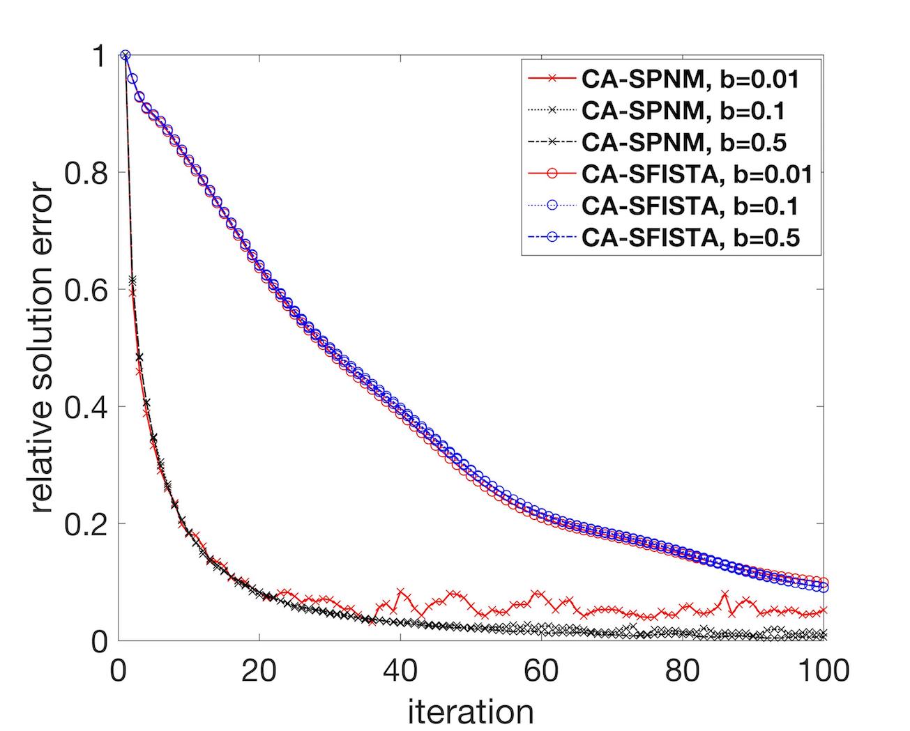
(b) covtype

Figure 2: Effect of $b$ on convergence and stability for abalone and covtype datasets; $k$ is set to 32.

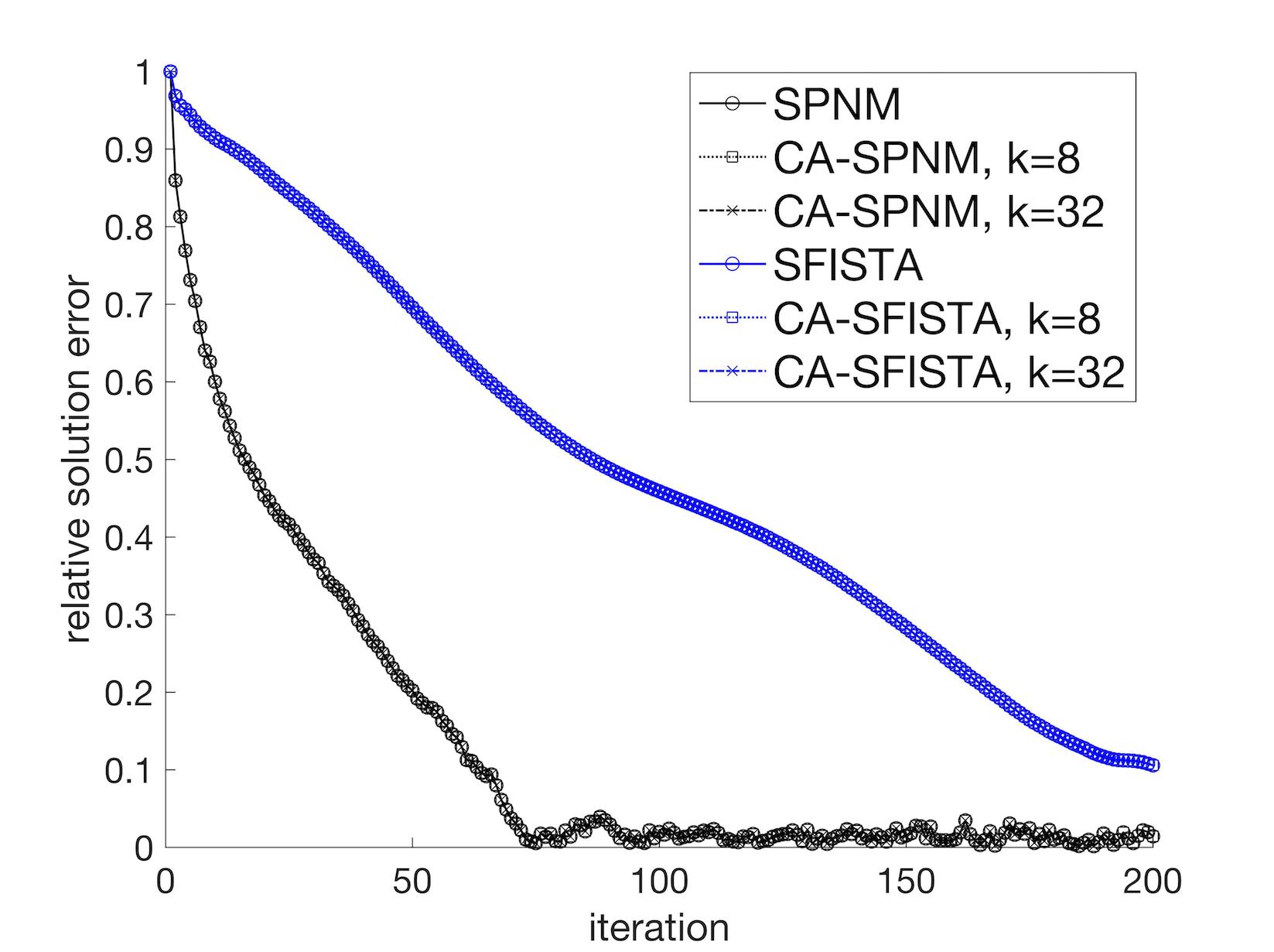
(a) abalone

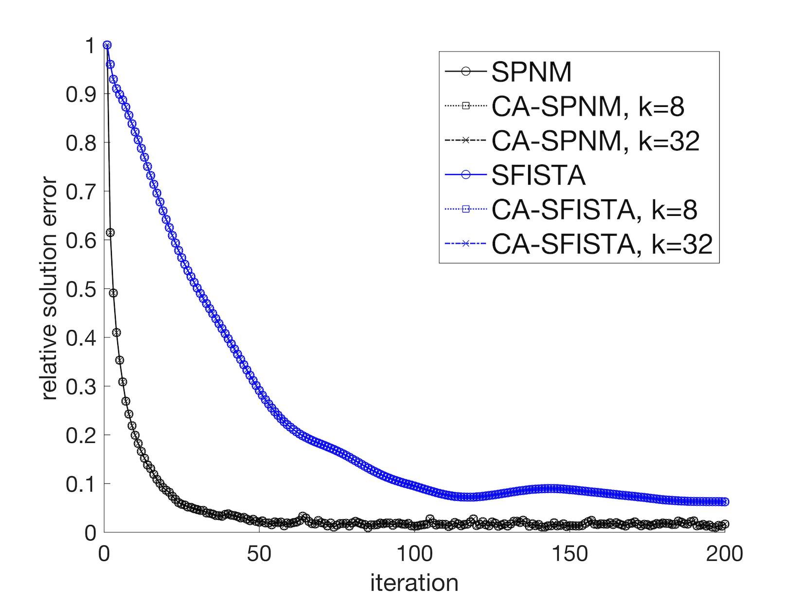
(b) covtype

Figure 3: Effect of $k$ on convergence and stability for abalone and covtype; $b=0.1$ for abalone and $b=0.01$ for covtype.

V-C Performance Experiments

Speedup and scaling results are presented in this section. Speedup results are obtained using the second stopping criteria and the tolerance parameter tol is set to 0.1 for all the experiments. For the scaling experiments, we use the first stopping criteria with 100 iterations to execute the same number of operations across the experiments. The largest dataset susy is executed on upto 1024 processors and the two smaller datasets abalone and covtype are executed on upto 64 and 512 processors respectively to report reasonable scalability based on size.

V-C1 Speedup

Figure 4 shows the speedup for all the datasets for different combinations of nodes (P) and k for CA-SFISTA. All the speedups are normalized over SFISTA. At small scale, for example for $P=8$ and k=32 for abalone in Figure 4a a speedup of 1.79X is achieved, while for the same dataset we can get a speedup of 9.63X on 64 nodes. Increasing $k$ significantly improves the performance of abalone since CA-SFISTA for a larger $k$ increases the ratio of floating point operations to communication for this relatively small data set on more processors.

As shown in the figure, the performance of all datasets almost always improves when increasing the number of nodes or k. For a fixed number of processors increasing $k$ reduces latency costs and communication without changing bandwidth or arithmetic costs. Figure 5 shows the speedup results for the CA-SPNM algorithm and follows a similar trend to CA-SFISTA. Figure 6 shows the speedup of CA-SFISTA and CA-SPNM algorithms on largest number of nodes for each dataset (64 for abalone, 512 for covtype, and 1024 for susy). Increasing k reduces the number of communicated massages and latency costs. Therefore, the speedups improve as k increases.

(a) abalone

(b) covtype

(c) susy

Figure 4: Speedup for CA-SFISTA algorithm on three different datasets.

(a) abalone

(b) covtype

(c) susy

Figure 5: Speedup for CA-SPNM algorithm on three different datasets.

Figure 6: speedups on largest number of nodes.

(a) CA-SFISTA

(b) CA-SPNM

Figure 7: Comparing execution time of CA-SFISA and CA-SPNM with the classical algorithms.

V-C2 Strong Scaling

Figure 7 (a) and Figure 7 (b) show strong scaling results for CA-SFISTA and CA-SPNM. The running times are the average over five runs for 100 iterations of the algorithm. The figures show the scaling behavior of the k-step algorithms for k=32 and compare it to SFISTA and SPNM. As shown in both figures, the classical algorithms do not scale well and their execution times increase when latency costs dominate. For example, for the abalone dataset, SFISTA’s running time increases on more than 8 processors, while CA-SFISTA continues to scale. The communication-avoiding methods are closer to ideal scaling. We intentionally added the $p=1024$ data point for the covtype dataset to Figure 7 to show that the performance of the $k$-step algorithms is bounded by bandwidth. This is because increasing k and the number of processors, increases the number of words to be moved in every k iterations and performance is bounded by the bandwidth of the machine. If the processors had no bandwidth limitations then the algorithms would scale for all increasing k.

VI Conclusion

Existing formulations of stochastic FISTA and proximal newton methods suffer from high communication costs and do not scale well on distributed platforms when operating on large datasets. We reformulate classical algorithms of SFISTA and SPNM to reduce inherent communication in their formulations. Our communication-avoiding algorithms leverage randomized sampling to overlap iterations and reduce communication costs by a factor of k. The proposed k-step algorithms do not change the classical algorithms’ convergence behavior and preserve the overall bandwidth and arithmetic costs. Our experiments show that CA-SFISTA and CA-SPNM provide up to 10X speedup for the tested datasets on distributed platforms.

References

- [1] L. Bottou, F. E. Curtis, and J. Nocedal, “Optimization methods for large-scale machine learning,” arXiv preprint arXiv:1606.04838, 2016.
- [2] I. Daubechies, M. Defrise, and C. De Mol, “An iterative thresholding algorithm for linear inverse problems with a sparsity constraint,” Communications on pure and applied mathematics, vol. 57, no. 11, pp. 1413–1457, 2004.
- [3] A. Beck and M. Teboulle, “A fast iterative shrinkage-thresholding algorithm for linear inverse problems,” SIAM journal on imaging sciences, vol. 2, no. 1, pp. 183–202, 2009.
- [4] J. D. Lee, Y. Sun, and M. Saunders, “Proximal newton-type methods for convex optimization,” in Advances in Neural Information Processing Systems, 2012, pp. 827–835.
- [5] J. Dongarra, J. Hittinger, J. Bell, L. Chacon, R. Falgout, M. Heroux, P. Hovland, E. Ng, C. Webster, and S. Wild, “Applied mathematics research for exascale computing,” Lawrence Livermore National Laboratory (LLNL), Livermore, CA, Tech. Rep., 2014.
- [6] G. Ballard, E. Carson, J. Demmel, M. Hoemmen, N. Knight, and O. Schwartz, “Communication lower bounds and optimal algorithms for numerical linear algebra,” Acta Numerica, vol. 23, pp. 1–155, 2014.
- [7] V. Smith, S. Forte, C. Ma, M. Takac, M. I. Jordan, and M. Jaggi, “Cocoa: A general framework for communication-efficient distributed optimization,” arXiv preprint arXiv:1611.02189, 2016.
- [8] B. Recht, C. Re, S. Wright, and F. Niu, “Hogwild: A lock-free approach to parallelizing stochastic gradient descent,” in Advances in neural information processing systems, 2011, pp. 693–701.
- [9] F. Zhou and G. Cong, “On the convergence properties of a -step averaging stochastic gradient descent algorithm for nonconvex optimization,” arXiv preprint arXiv:1708.01012, 2017.
- [10] Y. You, J. Demmel, K. Czechowski, L. Song, and R. Vuduc, “Ca-svm: Communication-avoiding support vector machines on distributed systems,” in IEEE International Parallel and Distributed Processing Symposium, 2015, pp. 847–859.
- [11] Z. A. Zhu, W. Chen, G. Wang, C. Zhu, and Z. Chen, “P-packSVM: Parallel primal gradient descent kernel svm,” in Proceedings of the 2009 Ninth IEEE International Conference on Data Mining, ser. ICDM ’09. Washington, DC, USA: IEEE Computer Society, 2009, pp. 677–686.
- [12] A. T. Chronopoulos and C. W. Gear, “On the efficient implementation of preconditioned s-step conjugate gradient methods on multiprocessors with memory hierarchy,” Parallel computing, vol. 11, no. 1, pp. 37–53, 1989.
- [13] A. Chronopoulos and C. Swanson, “Parallel iterative s-step methods for unsymmetric linear systems,” Parallel Computing, vol. 22, no. 5, pp. 623 – 641, 1996.
- [14] E. C. Carson, Communication-avoiding Krylov subspace methods in theory and practice. University of California, Berkeley, 2015.
- [15] E. Carson, N. Knight, and J. Demmel, “Avoiding communication in nonsymmetric lanczos-based krylov subspace methods,” SIAM Journal on Scientific Computing, vol. 35, no. 5, pp. S42–S61, 2013.
- [16] A. Devarakonda, K. Fountoulakis, J. Demmel, and M. W. Mahoney, “Avoiding communication in primal and dual block coordinate descent methods,” arXiv preprint arXiv:1612.04003, 2016.
- [17] R. Tibshirani, “Regression shrinkage and selection via the lasso,” Journal of the Royal Statistical Society. Series B (Methodological), pp. 267–288, 1996.
- [18] M. Schmidt, A. Niculescu-Mizil, K. Murphy et al., “Learning graphical model structure using l1-regularization paths,” in AAAI, vol. 7, 2007, pp. 1278–1283.
- [19] J. Mairal, F. Bach, J. Ponce, and G. Sapiro, “Online dictionary learning for sparse coding,” in Proceedings of the 26th annual international conference on machine learning. ACM, 2009, pp. 689–696.
- [20] V. Smith, S. Forte, M. I. Jordan, and M. Jaggi, “L1-regularized distributed optimization: A communication-efficient primal-dual framework,” arXiv preprint arXiv:1512.04011, 2015.
- [21] S. Rendle, D. Fetterly, E. J. Shekita, and B.-y. Su, “Robust large-scale machine learning in the cloud,” in Proceedings of the 22nd ACM SIGKDD International Conference on Knowledge Discovery and Data Mining. ACM, 2016, pp. 1125–1134.
- [22] K. Koh, S.-J. Kim, and S. Boyd, “An interior-point method for large-scale l1-regularized logistic regression,” Journal of Machine learning research, vol. 8, no. Jul, pp. 1519–1555, 2007.
- [23] S. H. Fuller and L. I. Millett, “Computing performance: Game over or next level?” Computer, vol. 44, no. 1, pp. 31–38, 2011.
- [24] D. Culler, R. Karp, D. Patterson, A. Sahay, K. E. Schauser, E. Santos, R. Subramonian, and T. Von Eicken, “Logp: Towards a realistic model of parallel computation,” in ACM Sigplan Notices, vol. 28, no. 7. ACM, 1993, pp. 1–12.
- [25] A. Alexandrov, M. F. Ionescu, K. E. Schauser, and C. Scheiman, “Loggp: incorporating long messages into the logp model—one step closer towards a realistic model for parallel computation,” in Proceedings of the seventh annual ACM symposium on Parallel algorithms and architectures. ACM, 1995, pp. 95–105.
- [26] L. Xiao and T. Zhang, “A proximal stochastic gradient method with progressive variance reduction,” SIAM Journal on Optimization, vol. 24, no. 4, pp. 2057–2075, 2014.
- [27] A. Nitanda, “Stochastic proximal gradient descent with acceleration techniques,” in Advances in Neural Information Processing Systems, 2014, pp. 1574–1582.
- [28] C.-C. Chang and C.-J. Lin, “Libsvm: a library for support vector machines,” ACM transactions on intelligent systems and technology (TIST), vol. 2, no. 3, p. 27, 2011.
- [29] J. Towns, T. Cockerill, M. Dahan, I. Foster, K. Gaither, A. Grimshaw, V. Hazlewood, S. Lathrop, D. Lifka, G. D. Peterson et al., “Xsede: accelerating scientific discovery,” Computing in Science & Engineering, vol. 16, no. 5, pp. 62–74, 2014.
- [30] S. R. Becker, E. J. Candès, and M. C. Grant, “Templates for convex cone problems with applications to sparse signal recovery,” Mathematical programming computation, vol. 3, no. 3, pp. 165–218, 2011.