Cooperative parametric resonance of the spin one half system of the dense atomic gas

Abstract

The cooperative resonance for a spin one half system interacting with dc and ac magnetic field is considered. This interaction in the system collective regime can result in parametic resonance and rapid excitation of the excited spin state of the dense atomic gas. The phenomenon is studied using the density matrix approach. We discuss the implementation of this effect and possible applications of the quantum amplification by superradiant emission of radiation.

I Introduction

The paradigm of two-level systems in an electromagnetic field plays an extremely important role in two quite different branches of physics, quantum optics and magnetic resonance theory. Using mathematical analogy, one can transfer the idea of the effect developed in one branch to another branch and a similar effect to predict. Thus, we have an exciting opportunity and playground for the implementation of proof-of-principle model experiment to demonstrate new effect in the branch where experimenting is easy. In this paper we analyze cooperative resonance in a spin one half system interacting with the magnetic field and demonstrate that this system can exhibit superradiant emission of radiation similar to that of recently discovered for the two-level atomic gas.

The so-called, quantum amplification by superradiant emission of radiation, a new concept of coherent radiation generation, was proposed in Refs.svidzinzki2013 ; genkin00pra ; mos . It is based on the cooperative effects in an ensemble of two-level atoms interacting with a radiation field in the resonator cavity book0 ; book . In order to explain the idea of new effect, we write the density matrix equations as

$$\dot{\rho}_{ab}=i(1-2\rho_{aa})\Omega_{s},$$ (1)

$$\dot{\Omega}_{s}=i\Omega_{a}^{2}\rho_{ab}.$$ (2)

Here $\Omega_{s}=\wp E_{s}/\hbar$ is the Rabi frequency of the radiation field coupled to the atomic ensemble, $\rho_{aa}$ is the atomic population in the excited state, $\rho_{ab}$ is the atomic coherence, and $\Omega_{a}$ is the cooperative frequency defined by

$$\Omega_{a}^{2}=\frac{2\pi}{\hbar}\omega_{ab}\wp^{2}N,$$

$N$ is the density of atoms.

We can represent Eqs. (1) and (2) in the following form:

$$\ddot{\Omega}_{s}+\Omega_{a}^{2}(1-2\rho_{aa})\Omega_{s}=0.$$ (3)

When two-levell atoms are in the excited state ($\rho_{aa}>1/2$), their transition to the ground state leads to the generation of a superradiant pulse dicke .

If the atoms are close to the ground state ($\rho_{aa}<1/2$), then Eq.(3) describes a harmonic oscillator. So far as the energy

$${\cal E}=\left(\hbar\omega_{ab}N\rho_{aa}+{|E_{s}|^{2}\over 4\pi}\right)V_{cavity}$$

stored in the atoms and the laser field is conserved, the radiation oscillates at the cooperative frequency $\Omega_{a}$ and the energy goes from the radiation to excite atoms and back.

The amplitude of this oscillation rapidly increases if the atomic population is modulated as $\rho_{aa}=\rho_{aa}^{0}+\delta\rho_{aa}\cos(2\nu t)$ near the cooperative frequency $\nu\approx\Omega_{a}$. In this case the equation for radiation (3) becomes the Mathieu equation, and we have the parametric resonance leading to the growth of the oscillation field amplitude. The energy increases due to interaction of the atomic gas with the external modulation field, which leads to the population excitation and simultaneously increases the laser field.

The above simple consideration showed that the cooperative resonance is a promising tool for the development of new sources for the coherent radiation generation. However, in order to build more realistic approach in the optical range, we have to take into account the velocity distribution of atoms. The cooperative frequency is not well-defined in this case and to observe the cooperative effects, some additional conditions are required. At the same time, we can develop similar models in the RF (or microwave) range. The interaction of intense ultrashort pulses with atomic system can be studied with RF pulses as a model system HLi10prl . We acknowledge also the ground-breaking experiments performed with RF radiation cohentannoudji . Such experiments in the RF region might furnish physical insight for the development of approaches using the cooperative resonances.

In this paper, we consider the cooperative resonance in the spin one half system coupled to the magnetic ac and dc field. The resonance with the cooperative frequency creates possibility to generate the magnetic field as well as to excite the system of spins. In particular, we consider a gas of two-level atoms in the presence of coherent driving field. The coherent field either has modulation at the cooperative frequency or detune off the resonance at the amount of the cooperative frequency.

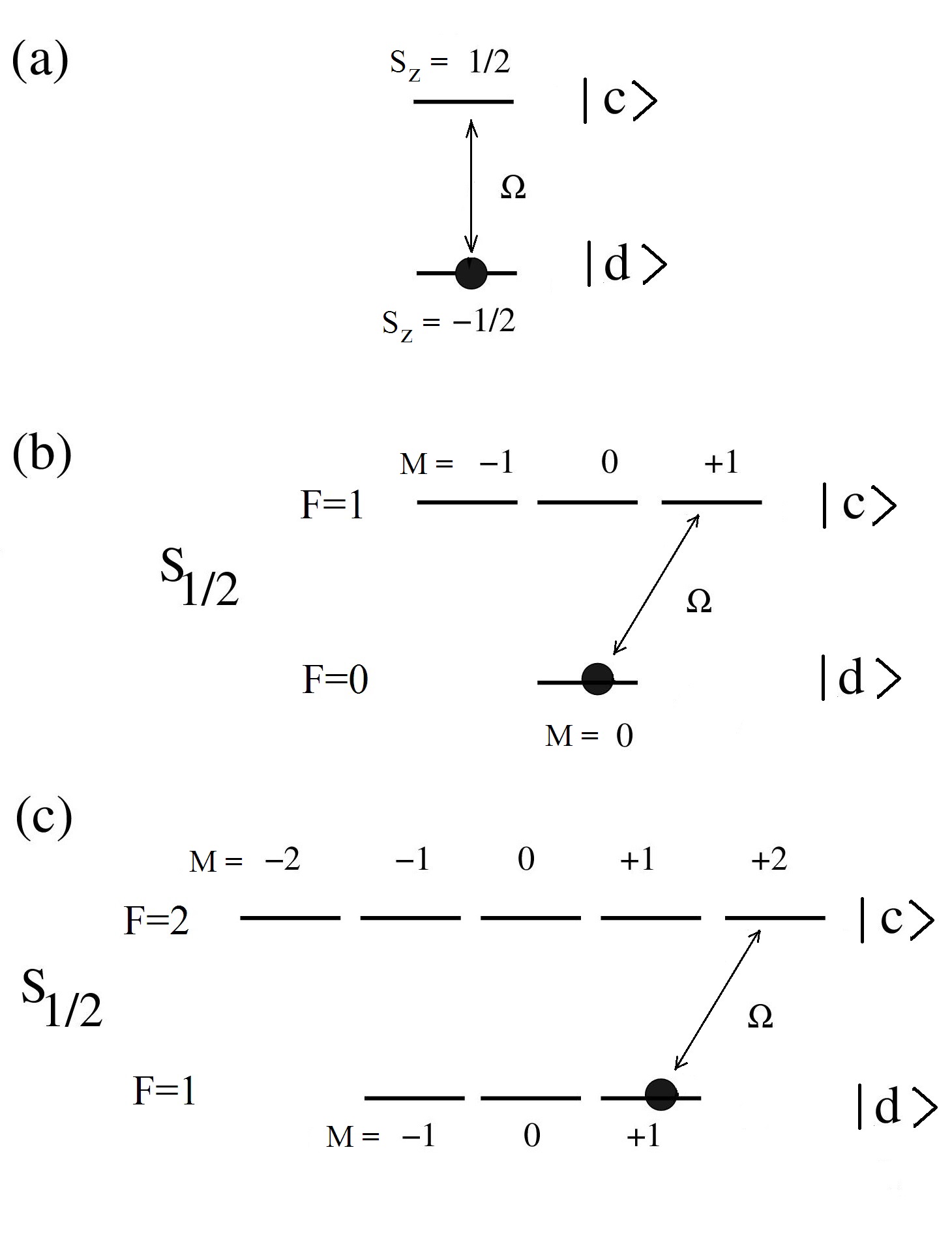
Figure 1: Level structure of (a) spin-1/2 system, (b) hydrogen atom, and (c) Rb atom. The population is optically pumped to the state $|d\rangle$, namely: (a) $|-1/2\rangle$, (b) $|F=0,M=0\rangle$, and (c) $|F=1,M=+1\rangle$.

II Model

In this section we consider a two-level system, spin-1/2, interacting with the circularly polarized magnetic field. Schematically this simple system is shown in Fig. 1a, and the basic equations are given in Appendix A.

In addition, we consider two examples of real two-level system in application to atoms, namely, hydrogen atom (see, Fig. 1b) and Rb atom (see, Fig. 1c).

One can optically pump all population to the particular state $|d\rangle$ (marked in Fig. 1a-c by a bullet) and then apply the circular polarized RF field between two levels as shown in the same figure. The frequency of the RF transitions can be controlled by a dc magnetic field.

The experiment can be performed with RF (or, microwave) fields. Note that another possible realization of the present results involves experiments with atoms in Rydberg states, as in kleppner , or using a RF field resulting in magnetic dipole transitions between levels with the same $F$ and different $M$ in the magnetic field cohentannoudji .

The spin Hamiltonian in the circular magnetic field $B_{x}=B_{s}\cos(\nu t)$ and $B_{y}=-B_{s}\sin(\nu t)$, is given by

$${\cal H}=\mu_{x}B_{x}+\mu_{y}B_{y}={B_{s}\over 2}[\mu_{+}e^{-i\nu t}+\mu_{-}e^{i\nu t}],$$ (4)

where $\mu_{\pm}=(\mu_{x}\pm i\mu_{y})/\sqrt{2}$ and ${\vec{\mu}}=\mu_{B}({\bf L}+2{\bf S})$ is the magnetic moment.

Evolution of the state vector

$$|\Psi\rangle=\sum_{FM}a_{FM}e^{-i\omega_{F}t}|FM\rangle,$$ (5)

is determined by the equation

$$i\dot{a}_{FM}={B_{0}\over 2\hbar}\sum_{F^{\prime}M^{\prime}}\left(\langle FM|\mu_{+}|F^{\prime}M^{\prime}\rangle\exp[-i(\nu+\omega_{F^{\prime}F}t)]+\langle FM|\mu_{-}|F^{\prime}M^{\prime}\rangle\exp[i(\nu-\omega_{F^{\prime}F}t)]\right)a_{F^{\prime}M^{\prime}}$$ (6)

The elements of matrices $\langle FM|\mu_{\pm}|F^{\prime}M^{\prime}\rangle$ and the explicit form of Eq. (6) can be found in Appendix B. To find the magnitization of the spins, we solve the set of Eqs. (6).

We can also use the following equations of motion for the density matrix $\rho$ at the times much shorter than the relaxation times:

$$\dot{\rho}_{aa}=2\Omega_{s}\mbox{Im}{\rho_{ab}},$$ (7)

$$\dot{\rho}_{ab}=i(1-2\rho_{aa})\Omega_{s}.$$

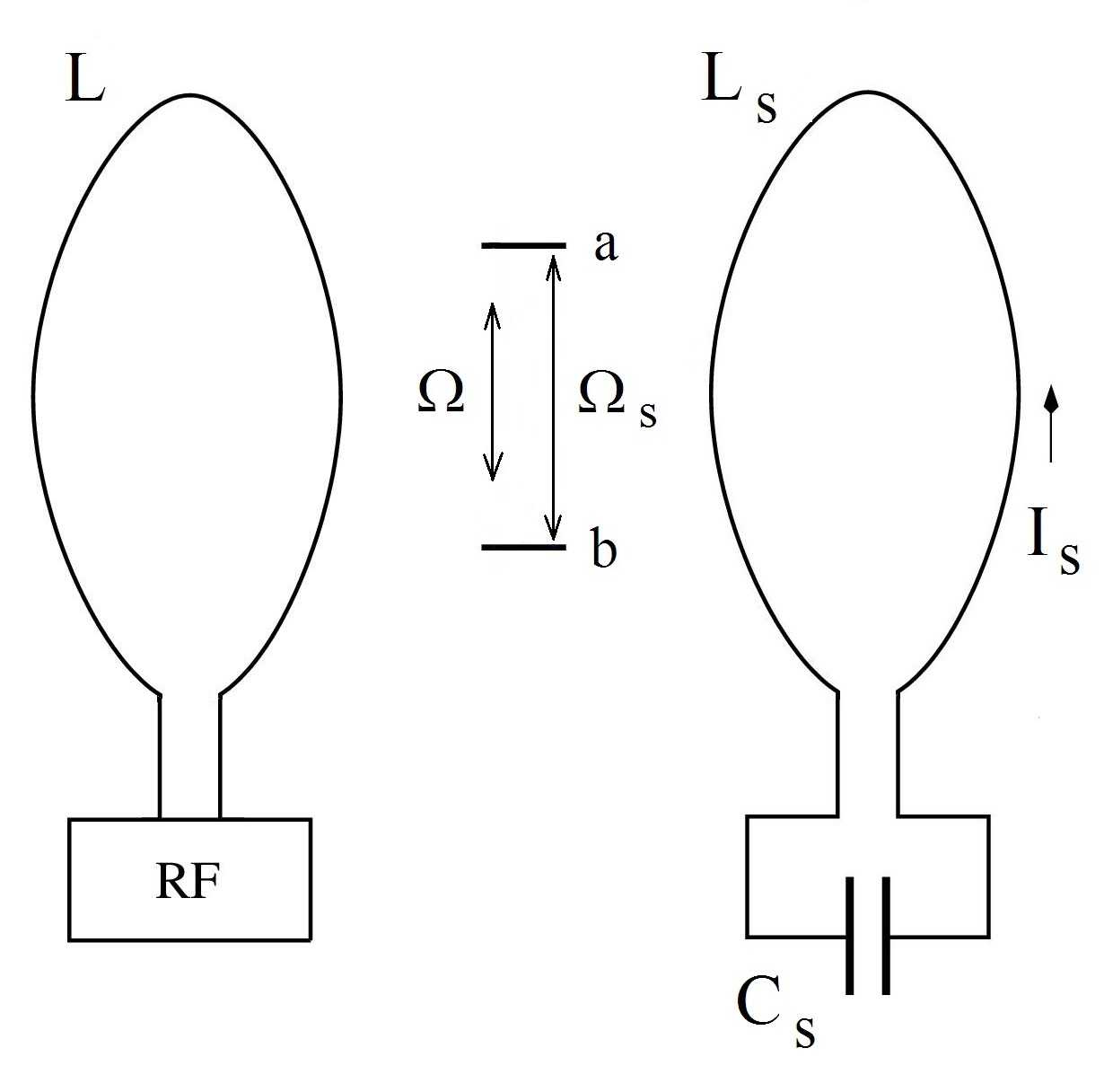
Figure 2: The configuration of the Zeeman sublevels driven by RF field $\Omega$ created by RF generator, and the RF field $\Omega_{s}$ generated in a resonant contour.

Now we turn our attention to the coupling of the induced magnetic polarization to the probe magnetic field $B_{s}$ that is created by the resonant RF circuit (with high quality factor Q), which consists of the inductance $L_{s}$ and a capacitor $C_{s}$ (see, Fig. 2) and has a resonant frequency at the frequency of the atomic a-b transition, is to be excited by Rb atoms.

It is possible to consider a proof-of-principle experiment to demonstrate the mechanism of radiation generation. Using the Zeeman splitting of hyperfine magnetic sublevels, one can drive the system with a detuned RF field (see Fig. 2, the RF generator drives current $I$ through the coil to create a magnetic field $B$. This field is defined by the relation $LI=A_{d}B$, where $L$ is the inductance and $A_{d}$ is the area of the coil.

The oscillating at the frequency $\omega$ magnetic dipole creates the electric field that in the case of $kr\ll 1$ is given byJackson

$$\vec{E}=-{\mu_{0}k^{2}\over 4\pi}\vec{n}\times\vec{\mu}{e^{ikr}\over r}\left(1+{i\over kr}\right)\simeq-i{\mu_{0}k\over 4\pi}{\vec{n}\times\vec{\mu}\over r^{2}},$$ (8)

where $\mu_{0}$ is the permeability of vacuum, $k=\omega/c$, $\vec{\mu}$ is the oscillating magnetic moment,

$$\vec{\mu}=\vec{\mu}_{ab}{\cal N}\rho_{ab}e^{-i\omega t},$$ (9)

${\cal N}=NV_{\mbox{sample}}$ is the number of the atomic spins, which depends on the spin density $N$ and the volume of the sample. For simplicity, let us consider the magnetic spins being in the center of a circle wire, and, then, the electromotive force generated in the electric circuit is given by

$$V=\oint_{{\cal L}_{s}}\vec{E}\cdot\vec{dl}=-i{\mu_{0}k\over 4\pi}\oint_{{\cal L}_{s}}{(\vec{n}\times\vec{\mu})\cdot\vec{dl}\over r^{2}}$$ (10)

$$=-i{\mu_{0}k\over 4\pi}\vec{\mu}\cdot\oint_{{\cal L}_{s}}{\vec{dl}\times\vec{n}\over r^{2}}=-i{\mu_{0}k\over 4\pi}\vec{\mu}\cdot\vec{\cal J},$$

where

$$\vec{\cal J}=\oint_{{\cal L}_{s}}{\vec{dl}\times\vec{n}\over r^{2}}.$$ (11)

The coil current $I_{s}$ is then given by

$$L_{s}\dot{I}_{s}+{q_{s}\over C_{s}}=V$$ (12)

and

$$\ddot{I}_{s}+\omega_{s}^{2}I_{s}={\dot{V}\over L_{s}},$$ (13)

where $\omega_{s}=({L_{s}C_{s}})^{-1/2}$.

The current $I_{s}$ and the magnetic field $B_{s}$ created by the coil follow from the Biot-Savart law

$$\vec{B}_{s}={\mu_{0}\over 4\pi}I_{s}\oint_{{\cal L}_{s}}\displaystyle{\vec{dl}\times\vec{r}\over r^{3}}={\mu_{0}\over 4\pi}I_{s}\vec{\cal J}.$$ (14)

One can write

$$\ddot{\vec{B}_{s}}+\omega_{s}^{2}\vec{B}_{s}={\mu_{0}\over 4\pi}{\dot{V}\over L_{s}}\vec{\cal J}=\displaystyle{\dot{V}\over 2a_{s}L_{s}},$$ (15)

or,

$$\ddot{\vec{B}_{s}}+\omega_{s}^{2}\vec{B}_{s}=-i{k\over L_{s}}\left({\mu_{0}\over 4\pi}\right)^{2}(\dot{\vec{\mu}}\cdot\vec{\cal J})\vec{\cal J}.$$ (16)

Using the slowly varying amplitude approaximation, $B_{s}=\tilde{B}_{s}e^{-i\omega_{s}t}$, we obtain

$$-2i\omega_{s}\dot{\tilde{B}}_{s}=-i{k_{s}\over L_{s}}\left({\mu_{0}\over 4\pi}\right)^{2}(\dot{\vec{\mu}}\cdot\vec{\cal J})\vec{\cal J}$$ (17)

where $k_{s}=\omega_{s}/c$ and

$$\dot{\tilde{B}}_{s}=-i{\omega_{s}\over 2cL_{s}}\left({\mu_{0}\over 4\pi}\right)^{2}(\vec{\mu}_{ab}\cdot\vec{\cal J})\vec{\cal J}{\cal N}\rho_{ab}.$$ (18)

Introducing $\Omega_{s}={\vec{\mu}_{ab}\cdot\tilde{B}_{s}/\hbar}$, one has

$$\dot{\Omega}_{s}=-i{\omega_{s}\over 2\hbar cL_{s}}\left({\mu_{0}\vec{\mu}_{ab}\cdot\vec{\cal J}\over 4\pi}\right)^{2}{\cal N}\rho_{ab}=-i\Omega_{a}^{2}\rho_{ab},$$ (19)

where

$$\Omega_{a}^{2}={\omega_{s}\over 2\hbar cL_{s}}\left({\mu_{0}\vec{\mu}_{ab}\cdot\vec{\cal J}\over 4\pi}\right)^{2}{\cal N}={\omega_{s}\mu_{0}^{2}\mu_{ab}^{2}{\cal N}\over 8\hbar cL_{s}a_{s}^{2}},$$ (20)

and $a_{s}$ is the radius of the coil.

III Cooperative parametric resonance

Let us consider theoretically the interaction of strong coherent field effects on the population of two atomic spin states of a dense atomic gas interacting in a collective regime. It is an interesting way of generation of a laser field that is not based on population inversion, but rather on the cooperative interaction with the ensemble of two-level atoms. The key feature of the approach is that the laser field is generated together with the population in the excited state.

To demonstrate the cooperative parametric resonance, we write the Rabi driving frequency in the rotating wave approximation as

$$\Omega=\Omega_{0}\cos(\nu t).$$ (21)

Introducing the phase

$$\theta=\int^{t}_{0}[\Omega_{s}+\Omega_{0}\cos(\nu t)]dt,$$ (22)

one can represent solutions of Eqs. (7) in the following form:

$$\rho_{aa} = \sin^{2}(\theta),$$ (23)

$$\rho_{ab} = {i\over 2}\sin(2\theta).$$ (24)

For a weak field one has $\theta\ll 1$ and therefore, $\rho_{aa}\simeq\theta^{2}$. In the beginning of lasing, we can neglect the change in phase due to the laser field: $\Omega_{s}t\simeq 0$. Then the population of the excited state can be expressed as

$$\rho_{aa}\approx{\epsilon^{2}\over 2}[1-\cos(2\nu t)],$$ (25)

where $\epsilon=\Omega_{0}/\nu$.

For the laser field Eq.(19), we obtain

$$\ddot{\Omega}_{s}=-\omega_{0}^{2}(1+\epsilon^{2}\cos 2\nu t)(\Omega_{s}+\Omega_{0}\cos\nu t)$$ (26)

where $\omega_{0}^{2}=\Omega_{a}^{2}(1-\epsilon^{2})$.

Let us try solution of Eq.(26) in the form

$$\Omega_{s}=A_{1}e^{i\nu t}+A_{2}e^{-i\nu t}.$$ (27)

Here $A_{1,2}$ are slowly varying amplitudes for which we get

$$\dot{A}_{1}=i\Delta A_{1}-iGA_{2}-i{\omega_{0}^{2}\Omega_{0}\over 2\nu},$$ (28)

$$\dot{A}_{2}=-i\Delta A_{2}+iGA_{1}+i{\omega_{0}^{2}\Omega_{0}\over 2\nu},$$ (29)

where $\Delta=(\nu^{2}-\omega_{0}^{2})/2\nu$ and $G=\epsilon\omega_{0}^{2}/2\nu$.

Now we are looking for the solution of the form $A_{1,2}\propto\exp(\lambda t)$ and obtain the following characteristic equation

$$(\lambda-i\Delta)(\lambda+i\Delta)-G^{2}=0.$$ (30)

The obtained characteristic numbers are:

$$\lambda=\pm\sqrt{G^{2}-\Delta^{2}}.$$ (31)

Thus, for $\Delta=0$, one can write the solution as

$$\left(\begin{array}[]{c}A_{1}\\ A_{2}\end{array}\right)={i-1\over 2G\nu}\omega_{0}^{2}\Omega_{0}\left(\begin{array}[]{c}1\\ i\end{array}\right)(1-e^{-Gt})$$ (36)

$$+{i+1\over 2G\nu}\omega_{0}^{2}\Omega_{0}\left(\begin{array}[]{c}1\\ -i\end{array}\right)(e^{Gt}-1),$$ (39)

that exhibits an exponential growth due to parametric resonance Landau89 .

To support the simplified calculations, we performed simulations of the set of Eq.(7) and Eq.(19). The results are shown in Fig. 3.

The parametric resonance leads to the growth of the probe field $\Omega_{s}/\Omega_{a}$ in the case of modulation of the atomic population in the excited state is shown vs $\Omega_{a}t$.

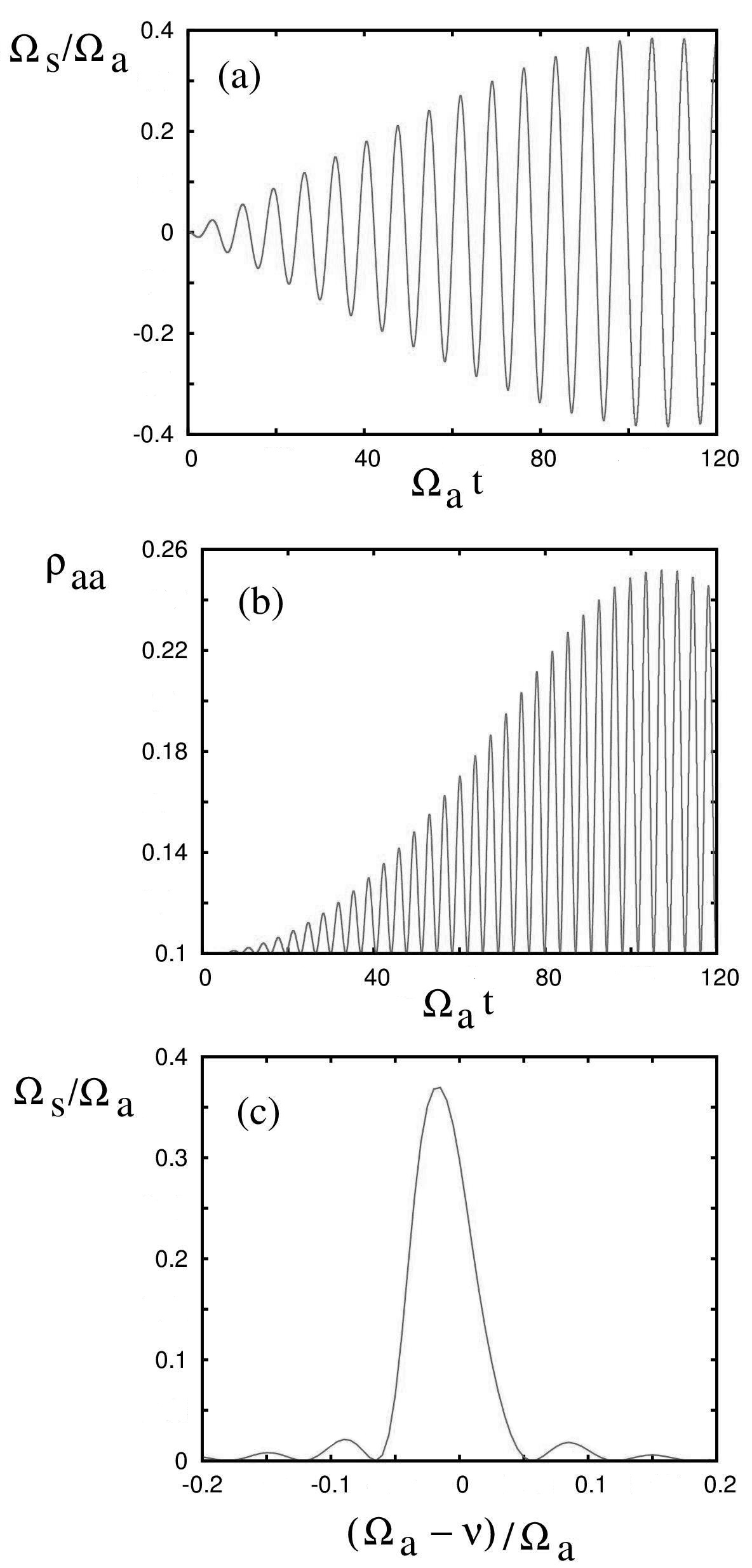
Figure 3: (a) The growth of the probe field $\Omega_{s}/\Omega_{a}$ versus dimensionless time $\Omega_{a}t$. (b) The growth of the population in the excited state $\rho_{aa}$ versus dimensionless time $\Omega_{a}t$. (c) The dependence of the growth of the probe field $\Omega_{s}/\Omega_{a}$ vs the detuning $(\Omega_{a}-\nu)/\Omega_{a}$. For simulation, the initial population in the excited state is $\rho_{aa}(0)=0.1$, and the drive amplitude is $\Omega_{0}=0.01\Omega_{a}$.

The excitation occurs at the cooperative resonance ($\nu\simeq\Omega_{a}$). As can be seen from Fig. 3, using a weak driving field $\Omega_{0}=0.01\Omega_{a}$, it is possible to excite the spin magnetization at almost the same the level ($\Omega_{a}\simeq 0.4\;\Omega_{a}$) as it would occured with superradiant generation corresponding to practically total population inversion.

This results can be observed in the experimental setup similar to the one described in HLi10prl . Using a longitudinal magnetic field $B=500$ G, the splitting is $\omega_{ab}\simeq 318.3$ MHz. Then, for the atomic density $N=10^{13}$ cm^-3, the cooperative frequency is $\Omega_{a}=10^{5}$ s^-1, which is much larger than the ground state relaxation $\gamma_{0}=3\cdot 10^{3}$ s^-1 ($\Omega_{a}\gg\gamma_{0}$).

The obtained above results can probably be applied to the nuclear spin systems (see, e.g., Ref. NMR ). It provides a new approach to the detection of nuclear magnetic resonance. Usually, NMR is detected by the measuring of additional losses in the coils at the nuclear. Meanwhile, the current approach allows one to induce the magnetic polarization the population difference is given by $\Delta N_{ab}=N_{0}{\Delta E/k_{B}T}$ where the density is $N_{0}\simeq 10^{23}$ cm^-3 the cooperative frequency is $\Omega_{a}=10^{4}$ s^-1. Then, modulation at the frequency $\Delta=\Omega_{a}$ leads to the strong magnetization of the nuclear transition.

We should mention another interesting opprotunity to find analogies (and therefore enrich our approach) using magnetic dynamics theory. The point is that the theory of parametric resonance of magnons, quanta of spin waves in magnetoordered systems is well-developed  safonov . So far as the roles of nonlinear medium and resonator cavity are theoretically well clarified in this branch of physics, a similar structure of dymamic equations gives useful hints how to update our simple model introducing new important parameters.

IV Discussion

In the paper, we study the new way of generation of coherent field based on the cooperative resonance in the system of spins which we consider as a good way to implement a proof-of-principle experimental realization as well as probably new way of nuclear magnetic resonance detection.

This new approach is not based on the population inversion which is required for lasing, as it is well-known to implement lasing, population inversion usually is needed to overcome stimulated absorption book0 . Also the technique is not related to the concept of lasing without population inversion (LWI) book that appears as a result of coherent effects ok86jetp ; fleisch05rmp ; sau05pra ; CPT ; book ; harris97phys2day in atomic or molecular media lwi1 ; lwi2 ; lwi3 . The LWI was demonstrated experimentally lwi1e ; lwi2e , and it was even shown that lasing can exist without any inversion in any reservoir, even under thermodynamical equilibrium ok98pra .

The physics of new way of generation is closely related to the cooperative response of quantum ensemble that are all practically in the ground state. Because of collective motion of the spin excitation at the cooperative frequency, the system undergoes the process of coherent excitation together with generation of coherent field. The physics is closely related to the so-called Dicke supperradiance dicke which is usually related to the spontaneous emission in the excited medium. Usually, spontaneous emission is an incoherent process that leads to relaxation of excitation in media. But in sufficiently dense media, the spontaneous emission becomes a collective process as was shown by Dicke dicke . The cooperative behavior of $N$ atoms can speed up the relaxation processes, leading to a burst of radiation with an intensity proportional to the square of the number of atoms $N^{2}$. Recently, in a single photon superradiance mos1 ; mos2 ; manassah08phl , the collective Lamb shift was predicted and observed mos3 ; LSh .

In conclusion, we have studied and demonstrated several cases when the resonance with the cooperative frequency creates the possibility to generate coherent radiation. In particular, we consider a gas of two-level atoms in the presence of either a CW or a pulsed coherent field that leads to substantial enhancement of the generated radiation under the condition that uses the cooperative frequency. A number of important applications of the generation of coherent radiation based on cooperative resonance phenomena that may lead to a significant progress in fundamental and applied physics.

Appendix A Spin one half system

The Hamiltonian for a spin-1/2 system in a magnetic field is defined by

$$\cal{H}=-{\vec{\mu}}\cdot{\bf B},$$ (40)

where

$${\vec{\mu}}=\mu_{B}(\sigma_{x}\hat{\bf x}+\sigma_{y}\hat{\bf y}+\sigma_{z}\hat{\bf z}).$$ (41)

Here the basis of two states, spin-up $|+\rangle$ and spin-down $|-\rangle$, is described by Pauli matrices

$$\sigma_{x}=\left(\begin{array}[]{cc}0&1\\ 1&0\end{array}\right),\;\sigma_{y}=\left(\begin{array}[]{cc}0&-i\\ i&0\end{array}\right),\;\sigma_{z}=\left(\begin{array}[]{cc}1&0\\ 0&-1\end{array}\right).$$ (42)

The magnetic field has a dc longitudinal component $B_{z}$ and the time-dependent transverse components

$${\bf B}=B_{z}\hat{\bf z}+B_{s}[\cos(\nu t)\hat{\bf x}+\sin(\nu t)\hat{\bf y}].$$ (43)

The longitudinal magnetic field causes splitting of the spin-up and spind-sown states as

$${\cal H}_{0}=\mu_{B}B_{z}\sigma_{z}=\mu_{0}B_{z}\left(\begin{array}[]{cc}1&0\\ 0&-1\end{array}\right).$$ (44)

The frequency, that corresponds to the transition between levels is defined by

$$\omega_{c}=2\mu_{B}B_{z}/\hbar.$$ (45)

The transverse magnetic field causes coupling between these states

$${\cal V}=\mu_{B}B_{s}e^{i{H_{0}t\over\hbar}}[\sigma_{x}\cos(\nu t))+\sigma_{y}\sin(\nu t)]e^{-i{H_{0}t\over\hbar}}.$$ (46)

Interaction Hamiltonian is given by

$${\cal V}=-\mu_{B}B_{s}e^{i{H_{0}t\over\hbar}}\left(\begin{array}[]{cc}0&e^{-i\nu t}\\ e^{i\nu t}&0\end{array}\right)e^{-i{H_{0}t\over\hbar}}$$ (47)

We see that the matrix elements,

$$\langle+|{\cal V}|-\rangle = -\mu_{B}B_{s}e^{-i(\nu-\omega_{c})t},$$ (48)

$$\langle-|{\cal V}|+\rangle = -\mu_{B}B_{s}e^{i(\nu-\omega_{c})t},$$ (49)

coinside with rotating wave approximation for the left-circularly polarized magnetic field. For the right-circularly polarized magnetic field the matrix elements are given by

$$\langle+|{\cal V}_{rcp}|-\rangle = -\mu_{B}B_{s}e^{-i(\nu+\omega_{c})t},$$ (50)

$$\langle-|{\cal V}_{rcp}|+\rangle = -\mu_{B}B_{s}e^{i(\nu+\omega_{c})t}.$$ (51)

Note that either the right-circularly or left-circularly polarized magnetic field is able to couple these two states.

For the linearly polarized transverse magnetic field

$${\bf B}=B_{s}{\bf x}\cos(\nu t)),$$ (52)

the matrix elements have the following form:

$$\langle+|{\cal V}|-\rangle=-\mu_{B}B_{s}[e^{-i(\nu-\omega_{c})t}+e^{i(\nu+\omega_{c})t}],$$ (53)

$$\langle-|{\cal V}|+\rangle=-\mu_{B}B_{s}[e^{i(\nu-\omega_{c})t}+e^{-i(\nu+\omega_{c})t}].$$ (54)

Appendix B Matrix elements of $\langle FM|\mu_{\pm}|F^{\prime}M^{\prime}\rangle$

For convenience to work with two-level H atom and Rb atom, here we derive the complete sets of equations.

B.1 H atom

The ¹H atom has a ground state split by a hyperfine interaction of electron and nuclear spins ($L=0$, $S=1/2$, $I=1/2$) in two levels with different total angular moment $F=L+S+I$, which has two values 0 and 1 as shown in Fig. 1b. The states are given by the elements of matrices $\langle FM|\mu_{\pm}|F^{\prime}M^{\prime}\rangle$, which can be calculated using

$$|F=1,M=1\rangle = |Sm_{s}=-1/2\rangle|Im_{i}=-1/2\rangle,\;\;|F=1,M=-1\rangle=|Sm_{s}=-1/2\rangle|Im_{i}=-1/2\rangle,$$ (55)

$$|F=1,M=0\rangle = {1\over\sqrt{2}}|Sm_{s}=-1/2\rangle|Im_{i}=1/2\rangle+{1\over\sqrt{2}}|Sm_{s}=1/2\rangle|Im_{i}=-1/2\rangle,$$ (56)

$$|F=0,M=0\rangle = {1\over\sqrt{2}}|Sm_{s}=-1/2\rangle|Im_{i}=1/2\rangle-{1\over\sqrt{2}}|Sm_{s}=1/2\rangle|Im_{i}=-1/2\rangle.$$ (57)

The nuclear magnetic moment can be neglected, because it is much smaller than the electron magnetic moment. We calculate thel elements of matrices as follows

$$\langle S,1/2|\mu_{+}|S,-1/2\rangle=\langle S,1/2|\mu_{-}|S,-1/2\rangle=\mu_{S},$$ (58)

where $\mu_{S}=g_{S}\mu_{B}$, $g_{s}=2$, and $\mu_{B}$ is the Bohr’s magneton. For example,

$$\langle F=1,M=1|\mu_{+}|F=1,M=0\rangle=\langle S,1/2|\langle I,1/2|\mu_{+}\left({1\over\sqrt{2}}|S,-1/2\rangle|I,1/2\rangle+{1\over\sqrt{2}}|S,1/2\rangle|I,-1/2\rangle\right)={\mu_{S}\over\sqrt{2}}.$$ (59)

Other elements can be calculated similarly:

$$-\langle F=0,M=0|\mu_{+}|F=1,M=-1\rangle=\langle F=0,M=0|\mu_{+}|F=1,M=1\rangle=\mu_{S},$$ (60)

$$\langle F=1,M=0|\mu_{+}|F=1,M=-1\rangle=\langle F=1,M=0|\mu_{+}|F=1,M=1\rangle=\mu_{S}.$$ (61)

Then, Eqs. (6) can be explicitely written as

$${d\over dt}\left(\begin{array}[]{c}a_{1-1}\\ a_{10}\\ a_{11}\\ a_{00}\end{array}\right)=\Omega_{0}\hat{L}\left(\begin{array}[]{c}a_{1-1}\\ a_{10}\\ a_{11}\\ a_{00}\end{array}\right),$$ (70)

where $\Omega_{0}=\mu_{B}B_{s}/\hbar$ and $\hat{L}$ is the following matrix

$$\left(\begin{array}[]{cccc}0&\Omega e^{i\nu t}&0&\Omega e^{-i(\nu+\omega_{c})t}\\ \Omega e^{-i\nu t}&0&\Omega e^{i\nu t}&0\\ 0&\Omega e^{-i\nu t}&0&\Omega e^{i(\nu-\omega_{c})}\\ \Omega e^{i(\nu+\omega_{c})t}&0&\Omega e^{-i(\nu-\omega_{c})}&0\end{array}\right).$$

This set of equations has been solved numerically.

B.2 Rb atom

The ⁸⁷Rb atom has a ground state split by a hyperfine interaction of electron and nuclear spins ($L=0$, $S=1/2$, $I=3/2$) in two levels with different total angular moment $F=L+S+I$, which has two values 1 and 2 as shown in Fig. 1c. The elements of matrices $\langle FM|\mu_{\pm}|F^{\prime}M^{\prime}\rangle$ can be calculated using

$$|F=1,M=-1\rangle = -{1\over 2}|Sm_{s}=-1/2\rangle|Im_{i}=-1/2\rangle+{\sqrt{3}\over 2}|Sm_{s}=1/2\rangle|Im_{i}=-3/2\rangle,$$ (71)

$$|F=1,M=0\rangle = -{1\over\sqrt{2}}|Sm_{s}=-1/2\rangle|Im_{i}=1/2\rangle+{1\over\sqrt{2}}|Sm_{s}=1/2\rangle|Im_{i}=-1/2\rangle,$$ (72)

$$|F=1,M=1\rangle = -{\sqrt{3}\over 2}|Sm_{s}=-1/2\rangle|Im_{i}=3/2\rangle+{1\over 2}|Sm_{s}=1/2\rangle|Im_{i}=1/2\rangle,$$ (73)

$$|F=2,M=-2\rangle = |Sm_{s}=-1/2\rangle|Im_{i}=-3/2\rangle,$$ (74)

$$|F=2,M=-1\rangle = {\sqrt{3}\over 2}|Sm_{s}=-1/2\rangle|Im_{i}=-1/2\rangle+{1\over 2}|Sm_{s}=1/2\rangle|Im_{i}=-3/2\rangle,$$ (75)

$$|F=2,M=0\rangle = {1\over\sqrt{2}}|Sm_{s}=-1/2\rangle|Im_{i}=1/2\rangle+{1\over\sqrt{2}}|Sm_{s}=1/2\rangle|Im_{i}=-1/2\rangle,$$ (76)

$$|F=2,M=1\rangle = {1\over 2}|Sm_{s}=-1/2\rangle|Im_{i}=3/2\rangle+{\sqrt{3}\over 2}|Sm_{s}=1/2\rangle|Im_{i}=1/2\rangle,$$ (77)

$$|F=2,M=2\rangle = |Sm_{s}=1/2\rangle|Im_{i}=3/2\rangle.$$ (78)

The nuclear magnetic moment can be neglected, because it is much smaller than the electron magnetic moment. We calculate all elements of matrixes as follows

$$\langle S,1/2|\mu_{+}|S,-1/2\rangle=\langle S,1/2|\mu_{-}|S,-1/2\rangle=\mu_{S},$$ (79)

where $\mu_{S}=g_{S}\mu_{B}$, $g_{s}=2$, and $\mu_{B}$ is the Bohr’s magneton. For example,

$$\langle F=2,M=2|\mu_{+}|F=1,M=1\rangle=\langle S,1/2|\langle I,3/2|\mu_{+}\left(-{\sqrt{3}\over 2}|S,-1/2\rangle|I,3/2\rangle+{1\over 2}|S,1/2\rangle|I,1/2\rangle\right)=-{\sqrt{3}\over 2}\mu_{S}.$$ (80)

Other elements can be calculated similarly

$$\langle F=2,M=2|\mu_{+}|F=2,M=1\rangle = {1\over 2}\mu_{S},\langle F=2,M=2|\mu_{+}|F=1,M=1\rangle=-{\sqrt{3}\over 2}\mu_{S},$$ (81)

$$\langle F=2,M=1|\mu_{+}|F=2,M=0\rangle = {\sqrt{6}\over 4}\mu_{S},\langle F=2,M=1|\mu_{+}|F=1,M=0\rangle=-{\sqrt{6}\over 4}\mu_{S},$$ (82)

$$\langle F=2,M=0|\mu_{+}|F=2,M=-1\rangle = {\sqrt{6}\over 4}\mu_{S},\langle F=2,M=0|\mu_{+}|F=1,M=-1\rangle=-{\sqrt{2}\over 4}\mu_{S},$$ (83)

$$\langle F=2,M=-1|\mu_{+}|F=2,M=-2\rangle = {1\over 2}\mu_{S},\langle F=1,M=1|\mu_{+}|F=1,M=0\rangle=-{\sqrt{2}\over 4}\mu_{S},$$ (84)

$$\langle F=1,M=0|\mu_{+}|F=1,M=-1\rangle = -{\sqrt{2}\over 4}\mu_{S},\langle F=1,M=1|\mu_{+}|F=2,M=0\rangle={\sqrt{2}\over 4}\mu_{S},$$ (85)

$$\langle F=1,M=0|\mu_{+}|F=2,M=-1\rangle = {\sqrt{6}\over 4}\mu_{S},\langle F=1,M=-1|\mu_{+}|F=2,M=-2\rangle={\sqrt{3}\over 2}\mu_{S}.$$ (86)

Then, Eqs. (6) can be explicitely written as

$${d\over dt}\left(\begin{array}[]{c}a_{1-1}\\ a_{10}\\ a_{11}\\ a_{2-2}\\ a_{2-1}\\ a_{20}\\ a_{21}\\ a_{22}\end{array}\right)=\Omega_{0}\hat{L}\left(\begin{array}[]{c}a_{1-1}\\ a_{10}\\ a_{11}\\ a_{2-2}\\ a_{2-1}\\ a_{20}\\ a_{21}\\ a_{22}\end{array}\right),$$ (103)

where $\Omega_{0}=\mu_{B}B_{s}/\hbar$ and $\hat{L}$ is the following matrix

$$\left(\begin{array}[]{cccccccc}0&-{\sqrt{2}\over 4}e^{i\nu t}&0&{\sqrt{3}\over 2}e^{-i(\nu+\omega_{c})t}&0&-{\sqrt{2}\over 4}e^{i(\nu-\omega_{c})t}&0&0\\ -{\sqrt{2}\over 4}e^{-i\nu t}&0&-{\sqrt{2}\over 4}e^{i\nu t}&0&{\sqrt{6}\over 4}e^{-i(\nu+\omega_{c})t}&0&-{\sqrt{6}\over 4}e^{i(\nu-\omega_{c})t}&0\\ 0&-{\sqrt{2}\over 4}e^{-i\nu t}&0&0&0&{\sqrt{2}\over 4}e^{-i(\nu+\omega_{c})t}&0&-{\sqrt{3}\over 2}e^{i(\nu-\omega_{c})t}\\ {\sqrt{3}\over 2}e^{i(\nu+\omega_{c})t}&0&0&0&{1\over 2}e^{i\nu t}&0&0&0\\ 0&{\sqrt{6}\over 4}e^{i(\nu+\omega_{c})t}&0&{1\over 2}e^{-i\nu t}&0&{\sqrt{6}\over 4}e^{i\nu t}&0&0\\ -{\sqrt{2}\over 4}e^{-i(\nu-\omega_{c})t}&0&{\sqrt{2}\over 4}e^{i(\nu+\omega_{c})t}&0&{\sqrt{6}\over 4}e^{-i\nu t}&0&{\sqrt{6}\over 4}e^{i\nu t}&0\\ 0&-{\sqrt{6}\over 4}e^{-i(\nu-\omega_{c})t}&0&0&0&{\sqrt{6}\over 4}e^{-i\nu t}&0&{1\over 2}e^{i\nu t}\\ 0&0&-{\sqrt{3}\over 2}e^{-i(\nu-\omega_{c})t}&0&0&0&{1\over 2}e^{-i\nu t}&0\end{array}\right).$$

References

• (1) A.A. Svizdinsky, L. Luqi, M.O. Scully, Phys. Rev. X 3, 041001 (2013).
• (2) G.M. Genkin, Phys. Rev. A 61, 055801 (2000).
• (3) M.O. Scully, The Qaser revisited: insights gleaned from analitical solutions to simple models, Laser Physics 24, 094014 (2014).
• (4) M. Sargent, M. O. Scully and W.E. Lamb, Laser Physics (Addison-Wesley, Reading, Massachusetts, USA, 1974).
• (5) M. O. Scully and M. S. Zubairy, Quantum Optics (Cambridge University Press, Cambridge, England, 1997).
• (6) R.H. Dicke, Phys. Rev. 93, 493 (1954).
• (7) H. Li, V.A. Sautenkov, Y.V. Rostovtsev, M.M. Kash, P.M. Anisimov, G.R. Welch, and M.O. Scully Phys. Rev. Lett. 104, 103001 (2010).
• (8) C. Cohen-Tannoudji, Optical Pumping and Interaction of Atoms with the Electromagnetic Field, in Cargese Lectures in Physics Vol. 2, edited by M. Levy (Gordon and Breach, New York, 1968), p.347.
• (9) J. R. Rubbmark, M.M. Kash, M.G. Littman, and D. Kleppner, Phys. Rev. A 23, 3107 (1981).
• (10) J.D. Jackson, Classical Electrodynamics (John Wiley & Sons, USA, NJ, 1999).
• (11) L.D. Landau, E.M. Lifschitz, Mechanics (Pergamon, Oxford, 1989).
• (12) V.I. Chizhik, Yu.S. Chernyshev, A.V. Donets, V.V. Frolov, A.V. Komolkin, and M.G. Shelyapina, Magnetic Resonance and Its Applications (Springer, Cham, 2014).
• (13) V.L. Safonov, Nonequilibrium Magnons: Theory, Experiment and Applications (Wiley-VCH, Weinheim, 2013).
• (14) O. Kocharovskaya, and Ya.I. Khanin, Sov. Phys. JETP 63, 945 (1986).
• (15) M. Fleischhauer, A. Imamoglu, and J. P. Marangos, Rev. Mod. Phys. 77, 633 (2005).
• (16) V.A. Sautenkov, Y.V. Rostovtsev, C. Y. Ye, G.R. Welch, O. Kocharovskaya, and M.O. Scully, Phys. Rev. A 71, 063804 (2005).
• (17) E. Arimondo, in Progress in Optics, edited by E. Wolf (Elsevier Science, Amsterdam, 1996), Vol. XXXV, p. 257.
• (18) S.E. Harris, Phys. Today 50, 36 (1997).
• (19) O.A. Kocharovskaya and Ya.I. Khanin, Pis’ma Zh. Exp. Teor. Fiz. 48, 581 (1988) [JETP Lett. 48, 630 (1988)].
• (20) S.E. Harris, Phys. Rev. Lett. 62, 1033 (1989).
• (21) M.O. Scully, S.-Y. Zhu, and A. Gavrielides, Phys. Rev. Lett. 62, 2813 (1989).
• (22) A.S. Zibrov, M.D. Lukin, D. E. Nikonov, L. Hollberg, M.O. Scully, V.L. Velichansky, and H.G. Robinson, Phys. Rev. Lett. 75, 1499 (1995).
• (23) G.G. Padmabandu, G.R. Welch, I.N. Shubin, E.S. Fry, D.E. Nikonov, M.D. Lukin, and M.O. Scully, Phys. Rev. Lett. 76, 2053 (1996).
• (24) O. Kocharovskaya, Y.V. Rostovtsev, I. Imamoglu, Phys. Rev. A 58, 649 (1998).
• (25) M.O. Scully, E. Fry, C.H.R. Ooi, K. Wodkiewicz, Phys. Rev. Lett. 96, 010501 (2006)
• (26) A.A. Svidzinsky, J. Chang, M.O. Scully, Phys. Rev. Lett. 100, 160504 (2008)
• (27) R. Friedberg, J.T. Manassah, Phys. Lett. A 372, 2514 (2008).
• (28) A.A. Svidzinsky, M.O. Scully, Science 325, 1510 (2009).
• (29) R. Rohlsberger, K. Schlage, B. Sahoo, S. Couet, and R. Ruffer, Science 328, 1248 (2010).