Nambu-Goldstone bosons characterized by the order parameter in spontaneous symmetry breaking

Abstract

We present explicitly a relation between the Nambu-Goldstone boson and the order parameter in non-relativistic systems with spontaneous symmetry breaking. We show that the Nambu-Goldstone bosons are characterized by transformation property of the order parameter under symmetry transformation of a system. We give an explicit formula for the Nambu-Goldstone boson for a general Lie group $G$, and then the number of the Nambu-Goldstone boson is derived straightforwardly from the form of the order parameter (the type of symmetry breaking). We show that the Ward-Takahashi identity is modified in the presence of the Nambu-Goldstone boson, where the generalized Ward-Takahashi identity includes the coupling (the vertex function) between fermions and Nambu-Goldstone bosons. The closed equation for the Green’s functions of Nambu-Goldstone bosons is derived by introducing the fermion-Nambu-Goldstone boson vertex function. Examples are given for $G=SU(2)$ (ferromagnetic), $U(1)$ (superconductor) and $SU(3)$ symmetry breaking.

I Introduction

Symmetry is important for a better understanding of the laws of nature. When the Lagrangian or the Hamiltonian is invariant under a symmetry transformation, we have a conserved current and a conserved quantity. When the Lagrangian is not invariant under some transformation, the corresponding conservation of the current is violated. There is often the case where the Lagrangian is invariant under a symmetry transformation, but the state is not invariant under this transformation. This means that an asymmetric state is realized in a symmetrical system. This is called the spontaneous symmetry breaking because it is a spontaneous process. When a continuous symmetry is broken spontaneously, a massless boson, called the Nambu-Goldstone boson (NG boson) emergesgold61 ; nam60 ; gold62 . Two general proofs of their existence were then given in Ref.gold62 ; wein . The spontaneous symmetry breaking has been an interesting subject since then in field theorycol85 ; nam61 ; hig64 ; wei72 ; gol66 ; bra10 ; nie76 ; wat11 ; wat12 ; hid13 ; oda13 ; wat14 ; nit15b and in the study of magnetism and superconductivity before thenand84 ; g-l ; bcs ; abs88 ; whi06 ; lep74 .

The Ward-Takahashi identity follows from the invariance of the Lagrangianwar50 ; tak57 . When the current conservation is violated by symmetry breaking, the Ward-Takahashi identity is never followed. The Ward-Takahashi identity is restored to hold, however, by means of the existence of the Nambu-Goldstone boson. This was examined in Ref.nam61 ; gri94 . The Ward-Takahashi identity is modified when the continuous symmetry is spontaneously broken.

Recently, the spontaneous symmetry breaking was classified into two groups Type I and Type IInie76 ; wat11 ; wat12 ; hid13 , and the dispersion relation of the Nambu-Goldstone boson was clarified following this classification. However, the relation between the Nambu-Goldstone boson and the order parameter is not clear since the theory is primarily based on the algebra of conserved quantities. The order parameter is important in the second-order phase transition which is realized as a spontaneous symmetry breaking. In this paper, we focus on the second-order phase transition, and show that the Nambu-Goldstone bosons are fully characterized by the transformation property of the order parameter $\Delta$ under symmetry trasformation of a system.

In this paper, we investigate the system with an invariance under the continuous transformation group $G$ (compact Lie group). We focus on non-relativistic models in this paper. The Nambu-Goldstone boson is expressed by means of the bases of Lie algebra of $G$ once the order parameter $\Delta$ is expressed as the expectation value of a boson field or a product of fermion fields. A new proof is given to show that the Nambu-Goldstone boson indeed represents a massless particle. Several proofs were given to show the existence of the Nambu-Goldstone boson when a continuous symmetry is spontaneously brokenwein . These proofs are, however, formal and abstract. It is helpful to give an explicit proof of the existence of the NG boson, and formulate the NG boson by means of fermion or boson fields explicitly.

We introduce a small symmetry breaking term in the Lagrangian (or the Hamiltonian) like the Zeeman term in a ferromagnet. When the ground states are degenerate continuously, operators $Q_{a}$, generators of transformation, are not well-defined in the Hilbert space. The symmetry breaking term, namely, the external field is introduced so that the ground state is unique and the matrix elements of $Q_{a}$ are defined. Lastly we take the vanishing limit of external field.

We also examine the Ward-Takahashi identity which is violated when there is a spontaneous symmetry breaking. The Ward-Takahashi identity is restored by including a contribution of the Nambu-Goldstone boson. In other words, the breaking of the Ward-Takahashi identity is compensated by the inclusion of the Nambu-Goldstone boson.

This paper is organized as follows. In the next section, we give a formulation of spontaneous symmetry breaking and give a formula for the Nambu-Goldstone boson $\pi_{a}$. We first examine a fermion system. We show that $\pi_{a}$ represents a massless boson. We give several examples of spontaneous symmetry breaking. In the section III, the Ward-Takahashi identity with the correction from the Nambu-Goldstone bosons is investigated, where the NG boson-fermion coupling (vertex function) is introduced. The equation for the Green’s function of NG bosons is obtained by using the NG boson-fermion vertex function. We give a summary in the last section.

II Nambu-Goldstone boson

II.1 Invariant Lagrangians

We consider models that are invariant under a continuous symmetry transformation of a Lie group $G$. A fermion Lagrangian is given in the form,

$$\mathcal{L}_{F}=\psi^{{\dagger}}i\Gamma^{\mu}\partial_{\mu}\psi+V(\psi),$$ (1)

where $\psi$ represents a fermion field. We can also examine a boson Lagrangian given as

$$\mathcal{L}_{B}=\phi^{{\dagger}}\left(i\hbar\frac{\partial}{\partial t}+\xi(\nabla)\right)\phi-V(\phi),$$ (2)

or the Lagrangian

$$\mathcal{L}_{B}=\frac{1}{2}\partial_{\mu}\phi^{{\dagger}}\partial^{\mu}\phi-V(\phi),$$ (3)

where $\phi$ is a scalar field, $V(\phi)$ is the potential term and $\xi(\nabla)$ is the dispersion relation.

We investigate a fermion system in the following. When the Lagrangian is invariant under the transformation $\psi\rightarrow\psi+\delta\psi$, we have the conserved current

$$j^{\mu}=\frac{\delta\mathcal{L}}{\delta(\partial_{\mu}\psi)}\delta\psi,$$ (4)

with $\partial_{\mu}j^{\mu}=0$. Let us denote the conserved currents as $j^{\mu}_{a}$ when there are several conserved currents and the corresponding conserved quantities as $Q_{a}$. Let us consider a Lie group (transformation group) $G$ and corresponding representation of fermion field $\psi$. Let $g$ be the Lie algebra of the Lie group $G$. We denote the basis set of the Lie algebra $g$ as $\{T_{a}\}$. We assume that $T_{a}$ is hermitian. The field transformation $\psi\rightarrow\psi+\delta\psi$ is given by

$$\psi\rightarrow e^{-i\theta T_{a}}\psi=\psi-i\theta T_{a}\psi+O(\theta^{2}),$$ (5)

where $\theta$ is an infinitesimal parameter. We write

$$\delta\psi=-i\theta T_{a}\psi,$$ (6)

and define the conserved quantities as

$$Q_{a}=\int d{\bf r}J_{a}^{0}({\bf r}),$$ (7)

where we set

$$J_{a}^{\mu}=\frac{1}{\theta}j_{a}^{\mu}.$$ (8)

We put $\Gamma^{0}=1$ for simplicity to obtain

$$[Q_{a},\psi]=-T_{a}\psi,$$ (9)

and

$$Q_{a}=\int d{\bf r}\psi^{{\dagger}}T_{a}\psi.$$ (10)

II.2 Spontaneous Symmetry Breaking

Let us introduce the term to the Lagrangian, which breaks the symmetry:

$$\mathcal{L}_{SB}=\lambda\psi^{{\dagger}}M\psi,$$ (11)

where $M$ is a c-number hermitian matrix in $\{T_{a}\}$. $\lambda$ is an infinitesimal real number and we let $\lambda\rightarrow 0$ at the end of calculations. $\mathcal{L}_{SB}$ is the external field such the Zeeman term in a ferromagnet. We denote the total Hamiltonian including the symmetry breaking term as $H_{T}$. We assume that the ground state of $H_{T}$ is unique, so that we avoid the difficulty stemming from the degeneracy of ground statesryd96 . If the ground state is not unique, we must add another symmetry breaking term to the Lagrangian to lift the degeneracy.

We define the order parameter $\Delta$ as the expectation value of this term:

$$\Delta=\langle\psi^{{\dagger}}M\psi\rangle.$$ (12)

We define that the symmetry generated by $Q_{a}$ with $[T_{a},M]\neq 0$ is spontaneously broken when $\Delta$ is finite $(\neq 0)$ in the limit $\lambda\rightarrow 0$. The susceptibility $\chi_{\Delta}$ is define as

$$\chi_{\Delta}=\lim_{\lambda\rightarrow 0}\frac{\Delta}{\lambda}.$$ (13)

$\chi_{\Delta}$ diverges when there is a spontaneous symmetry breaking.

Under the transformation $\psi\rightarrow\psi-i\theta T_{a}\psi$, $\mathcal{L}_{SB}$ transforms to $\mathcal{L}_{SB}+\delta\mathcal{L}_{SB}$ where

$$\delta\mathcal{L}_{SB}=i\theta\lambda\psi^{{\dagger}}[T_{a},M]\psi.$$ (14)

In this case, the current $j^{\mu}$ is not conserved:

$$\partial_{\mu}j_{a}^{\mu}=\delta\mathcal{L}_{SB}.$$ (15)

Then we have

$$\partial_{\mu}J_{a}^{\mu}=i\lambda\psi^{{\dagger}}[T_{a},M]\psi.$$ (16)

The divergence $\partial_{\mu}J^{\mu}_{a}$ is nothing but a Nambu-Goldstone boson. We define the Nambu-Goldstone boson as

$$\pi_{a}=i\psi^{{\dagger}}[T_{a},M]\psi.$$ (17)

This means

$$\partial_{\mu}J_{a}^{\mu}=\lambda\pi_{a}.$$ (18)

We show that $\pi_{a}$ indeed indicates a massless boson in the subsection 2.4.

Similarly, the Nambu-Goldstone in a boson system emerges. We introduce the symmetry breaking term $\mathcal{L}_{SB}$ to the Lagrangian $\mathcal{L}_{B}$. For example, we add

$$\mathcal{L}_{SB}=\lambda(\phi+\phi^{{\dagger}}).$$ (19)

Examples of scalar field theories are discussed in the subsection 2.3.

II.3 Examples of Symmetry Breaking

We show several examples of spontaneous symmetry breaking on the basis of our formulation in this subsection.

II.3.1 Ferromagnetic transition

We consider the fermion Lagrangian in Eq.(1) where $\psi$ is given by a doublet of fermions:

$$\psi(x) = \left(\begin{array}[]{c}\psi_{\uparrow}(x)\\ \psi_{\downarrow}(x)\\ \end{array}\right).$$ (22)

Here $\psi_{\sigma}$ represents the annihilation operator of fermion with spin $\sigma$. The symmetry group is $G=SU(2)$ and the bases $\{T_{a}\}$ are given by Pauli matrices $T_{a}=\sigma_{a}$ ($a=1,2$ and 3). The structure constants are $f_{abc}=2\epsilon_{abc}$. The Lagrangian is invariant under the transformations

$$\psi\rightarrow e^{-i\theta\sigma_{a}}\psi,$$ (23)

for $a=1,2$ and 3. The symmetry breaking term is given by the magnetization of electrons:

$$\mathcal{L}_{SB}=\lambda\psi^{{\dagger}}\sigma_{3}\psi=\lambda(\psi^{{\dagger}}_{\uparrow}\psi_{\uparrow}-\psi^{{\dagger}}_{\downarrow}\psi_{\downarrow}).$$ (24)

When $\Delta\equiv\langle\psi^{{\dagger}}\sigma_{3}\psi\rangle\neq 0$ in the limit $\lambda\rightarrow 0$, the symmetry is broken spontaneously. Since $[\sigma_{1},\sigma_{3}]\neq 0$ and $[\sigma_{2},\sigma_{3}]\neq 0$, this term breaks the symmetry $\psi\rightarrow e^{-i\theta\sigma_{a}}\psi$ for $a=1,2$. The Nambu-Goldstone bosons are

$$\pi_{1} = i\psi^{{\dagger}}[\sigma_{1},\sigma_{3}]\psi=2\psi^{{\dagger}}\sigma_{2}\psi,$$

$$\pi_{2} = i\psi^{{\dagger}}[\sigma_{2},\sigma_{3}]\psi=-2\psi^{{\dagger}}\sigma_{1}\psi.$$ (25)

The excitation mode represented by $\pi_{1}$ and $\pi_{2}$ is spin-flip process, that is, the spin-wave excitation. We make a linear combination of $\pi_{1}$ and $\pi_{2}$ as $\pi\equiv(i\pi_{1}-\pi_{2})/4=\psi^{{\dagger}}_{\uparrow}\psi_{\downarrow}$ and $\pi^{{\dagger}}=(-i\pi_{1}-\pi_{2})/4=\psi^{{\dagger}}_{\downarrow}\psi_{\uparrow}$. Actually, there is only one Nambu-Goldstone boson $\pi$ in a ferromagnetic state.

II.3.2 Antiferromagnetic transition

In the case of antiferromagnetic transition, we divide the space into two sublattices called A and B. We adopt that electrons are on a bipartite lattice. We denote the fermion fields on A and B sublattices as $\psi_{A}$ and $\psi_{B}$, respectively. We have $SU(2)$ symmetry in each sublattice. The symmetry breaking term is

$$\mathcal{L}_{SB}=\lambda\psi^{{\dagger}}_{A}\sigma_{3}\psi_{A}+\lambda\psi^{{\dagger}}_{B}\sigma_{3}\psi_{B}.$$ (26)

The order parameters are $\Delta_{A}=\langle\psi^{{\dagger}}_{A}\sigma_{3}\psi_{A}\rangle$ and $\Delta_{B}=\langle\psi^{{\dagger}}_{B}\sigma_{3}\psi_{B}\rangle$ with the constraint $\Delta_{A}+\Delta_{B}=0$ in the antiferromagnetic case. In a similar way as in the ferromagnetic case, $\pi=(i\pi_{1}-\pi_{2})/4$ (and its conjugate $\pi^{{\dagger}}$) is the Nambu-Goldstone boson in each sublattice. Thus we have two NG bosons $\pi_{A}$ and $\pi_{B}$ in this case.

II.3.3 Scalar field theories

(a) Single-component scalar field
Let us consider a complex scalar field model with the Lagrangian,

$$\mathcal{L}=\phi^{{\dagger}}\left(i\hbar\frac{\partial}{\partial t}+\frac{\hbar^{2}}{2m}\nabla^{2}+\mu\right)\phi(x)-\frac{g_{\phi}}{2}\phi^{{\dagger}}(x)\phi^{{\dagger}}(x)\phi(x)\phi(x),$$ (27)

where $g_{\phi}$ is the coupling constant, $x=(t,{\bf r})$ and we set $\hbar=1$. The Lagrangian is invariant under the transformation

$$\phi\rightarrow e^{-i\theta}\phi.$$ (28)

The conserved current is given by $j^{0}=i\phi^{{\dagger}}\delta\phi=\theta\phi^{{\dagger}}\phi$, and $j^{k}=-(1/2m)(\partial_{k}\phi^{{\dagger}})\delta\phi=i\theta(1/2m)(\partial_{k}\phi^{{\dagger}})\phi$ ($k=1$, 2 and 3). We define $J^{\mu}=j^{\mu}/\theta$ so that

$$J^{0}=\phi^{{\dagger}}\phi,~{}~{}J^{k}=i\frac{1}{2m}\left(\partial_{k}\phi^{{\dagger}}\right)\phi.$$ (29)

We include the symmetry breaking term:

$$\mathcal{L}_{SB}=\lambda(\phi+\phi^{{\dagger}}).$$ (30)

The divergence of the current is $\partial_{\mu}j^{\mu}=\delta\mathcal{L}_{SB}=-i\lambda\theta(\phi-\phi^{{\dagger}})$. The order parameter is

$$\Delta=\langle\phi+\phi^{{\dagger}}\rangle.$$ (31)

Since $\partial_{\mu}J^{\mu}=\lambda\pi$, the Nambu-Goldstone boson is given as

$$\pi=i(\phi^{{\dagger}}-\phi).$$ (32)

(b) Multi-component real scalar field
A symmetry breaking in a system with a multi-component model is similarly examined. For example, let us turn to a real three-component scalar field $\phi=^{t}(\phi_{1},\phi_{2},\phi_{3})$ with the Lagrangian

$$\mathcal{L}=\frac{1}{2}(\partial_{\mu}\phi_{i})(\partial^{\mu}\phi_{i})-V(\phi),$$ (33)

where the summation convention is applied and $V(\phi)$ is the potential. We assume that the Lagrangian is invariant under the action of $G=SO(3)$. The bases of the Lie algebra of $SO(3)$ are

$$J_{x}=\left(\begin{array}[]{ccc}0&0&0\\ 0&0&-i\\ 0&i&0\\ \end{array}\right), J_{y}=\left(\begin{array}[]{ccc}0&0&i\\ 0&0&0\\ -i&0&0\\ \end{array}\right),$$ (40)

$$J_{z} = \left(\begin{array}[]{ccc}0&-i&0\\ i&0&0\\ 0&0&0\\ \end{array}\right).$$ (44)

Let us adopt that there occurs a spontaneous symmetry breaking. We choose the symmetry breaking term as

$$\mathcal{L}_{SB}=\lambda\phi_{3}.$$ (45)

$\mathcal{L}_{SB}$ is invariant under the transformation $\phi\rightarrow e^{iJ_{z}\theta_{z}}\phi$. For the transformation $\phi\rightarrow e^{iJ_{x}\theta_{x}}\phi$, however, we have

$$\delta\mathcal{L}_{SB}=-\lambda\theta_{x}\phi_{2}.$$ (46)

Similarly,

$$\delta\mathcal{L}_{SB}=\lambda\theta_{y}\phi_{1},$$ (47)

under the transformation $\phi\rightarrow e^{iJ_{y}\theta_{y}}\phi$. Then, we have two massless bosons $\phi_{1}$ and $\phi_{2}$ and one massive scalar field $\phi_{3}$. For example, This is easily seen for the potential

$$\mathcal{L}=\frac{1}{2}(\partial_{\mu}\phi_{i})(\partial^{\mu}\phi_{i})-\frac{m^{2}}{2}\phi_{i}\phi_{i}-g(\phi_{i}\phi_{i})^{2},$$ (48)

with $m^{2}<0$ and $g>0$ by expanding the potential $V$ around the minimum.

(c) Multi-component complex scalar field
A model with a complex multi-component scalar field exhibits similar symmetry breaking. Let us consider a complex three-component scalar field theory given as

$$\mathcal{L}=\partial_{\mu}\phi^{{\dagger}}\partial^{\mu}\phi-\frac{m^{2}}{2}\phi^{{\dagger}}\phi-g(\phi^{{\dagger}}\phi)^{2},$$ (49)

where $\phi=^{t}(\phi_{1},\phi_{2},\phi_{3})$ and $g>0$. The Lagrangian has a $SU(3)$ symmetry. The bases are given by the Gell-Mann matrices $\lambda_{a}$ ($a=1,\cdots,8$): $\{T_{a}=\lambda_{a}/2\}$geo99 . We adopt $m^{2}<0$ and consider the symmetry breaking term given by

$$\mathcal{L}_{SB}=\lambda(\phi_{3}+\phi^{{\dagger}}_{3}).$$ (50)

This term is not invariant under the tranformation $\phi\rightarrow e^{iT_{a}\theta_{a}}\phi$ for $a=4$, 5, 6, 7 and 8. Thus, after spontaneous symmetry breaking, we have five massless Nambu-Goldstone bosons and one massive scalar field. The massive boson is $\phi_{3}+\phi^{{\dagger}}_{3}$ with the mass $8ga^{2}$ for $a=Re\langle\phi_{3}\rangle$, and massless bosons are $\phi_{1}$, $\phi_{2}$ and $i(\phi_{3}-\phi^{{\dagger}}_{3})$. The number of massless bosons is obtained straightforwardly in our formulation.

II.3.4 Superconducting transition

To discuss a superconducting transition, we use the Nambu representation $\psi=^{t}(\psi_{\uparrow},\psi^{{\dagger}}_{\downarrow})$. Let us consider a non-relativistic model of superconductivity given by

$$\mathcal{L}=i\psi^{{\dagger}}\partial_{t}\psi-\psi^{{\dagger}}\sigma_{3}\xi(\nabla))\psi-g\psi^{{\dagger}}_{\uparrow}(x)\psi_{\uparrow}(x)\psi^{{\dagger}}_{\downarrow}(x)\psi_{\downarrow}(x),$$ (51)

where the last term with the coupling constant $g<0$ is an attractive interaction term. This Lagrangian is invariant under the transformation

$$\psi\rightarrow e^{-i\theta\sigma_{3}}\psi.$$ (52)

This is the $U(1)$ phase transformation: $\psi_{\sigma}\rightarrow e^{-i\theta}\psi_{\sigma}$. We add the following symmetry breaking term

$$\mathcal{L}_{SB}=\lambda\psi^{{\dagger}}\sigma_{1}\psi=\lambda(\psi^{{\dagger}}_{\uparrow}\psi^{{\dagger}}_{\downarrow}+\psi_{\downarrow}\psi_{\uparrow}),$$ (53)

so that the invariance is lost. Then from the general theory the NG boson $\pi$ is given as

$$\pi=i\psi^{{\dagger}}[\sigma_{3},\sigma_{1}]\psi=2i(\psi^{{\dagger}}_{\uparrow}\psi^{{\dagger}}_{\downarrow}-\psi_{\downarrow}\psi_{\uparrow}).$$ (54)

$\pi$ is shown to be a massless boson following the argument in the subsection 2.4.

II.3.5 A multi-component fermion model

We can also consider a multi-component fermion field. Let us consider a fermion triplet ${}^{t}\psi=(\psi_{1},\psi_{2},\psi_{3})$. The symmetry group is $G=SU(3)$ and $\{T_{a}\}$ are given by the Gell-Mann matrices. We add the symmetry breaking term

$$\mathcal{L}_{SB}=\lambda\psi^{{\dagger}}T_{3}\psi,$$ (55)

for the symmetry breaking $\langle\psi^{{\dagger}}T_{3}\psi\rangle\neq 0$. Then the system is invariant under the transformation by $T_{3}$ and $T_{8}$. NG bosons are given by $\pi_{a}=i\psi^{{\dagger}}[T_{a},T_{3}]\psi$. Because the structure constants are given by $f_{123}=1$ and $f_{345}=-f_{367}=1/2$, there are three NG bosons:

$$\pi_{1}=\psi^{{\dagger}}T_{2}\psi,~{}~{}\pi_{4}=\frac{1}{2}\psi^{{\dagger}}T_{5}\psi,~{}~{}\psi_{6}=-\frac{1}{2}\psi^{{\dagger}}T_{7}\psi.$$ (56)

$\pi_{2}$, $\pi_{5}$ and $\pi_{7}$ are also NG bosons, but these are not independent.

When the symmetry breaking is given by $\langle\psi^{{\dagger}}T_{8}\psi\rangle\neq 0$, the symmetry group $G$ reduces to $H=\{T_{1},T_{2},T_{3},T_{8}\}$. In this case, we have two NG bosons.

II.4 Proof that $\pi_{a}$ is an NG Boson

The pole of the Green’s function gives information on the energy spectrum of the particleagd . Thus, we investigate the Green’s function in the following.

The normalization of $\{T_{a}\}$ is given as

$${\rm Tr}T_{a}T_{b}=c\delta_{ab},$$ (57)

where $c$ is a real constant: $c\in{\bf R}$. The commutators are

$$[T_{a},T_{b}]=\sum_{c}if_{abc}T_{c},$$ (58)

where $f_{abc}$ are structure constants of the Lie algebra $g$. We use the relation

$$\sum_{ab}f_{abc}f_{abd}=C_{2}(G)\delta_{cd},$$ (59)

where $C_{2}(G)$ indicates the Casimir invariant of the Lie group $G$. $C_{2}(G)$ is given by

$$C_{2}(G) = 2Nc~{}~{}{\rm for}~{}G=SU(N)$$ (60)

$$= (N-2)c~{}~{}{\rm for}~{}G=O(N).$$ (61)

For example, for $SU(2)$, we have $C_{2}(G)=8$ when we use $c=2$. The above relation results in

$$\sum_{a}[T_{a},[T_{a},T_{b}]]=\sum_{acd}f_{acb}f_{acd}T_{d}=C_{2}(G)T_{b}.$$ (62)

Let $M$ be an element of the basis set of $g$: $M=T_{m}\in\{T_{a}\}$. From Eq.(9), we have

$$e^{i\theta Q_{a}}\psi^{{\dagger}}e^{-i\theta Q_{a}}[M,T_{a}]e^{i\theta Q_{a}}\psi e^{-i\theta Q_{a}}$$

$$~{}~{}=\psi^{{\dagger}}[M,T_{a}]\psi+i\theta\psi^{{\dagger}}[T_{a},[M,T_{a}]]\psi+O(\theta^{2})$$

$$~{}~{}=-i\sum_{c}f_{amc}\psi^{{\dagger}}T_{c}\psi-i\theta\sum_{cd}f_{acm}f_{acd}\psi^{{\dagger}}T_{d}\psi+O(\theta^{2}).$$

We assume that $\langle\psi^{{\dagger}}T_{m}\psi\rangle=\langle\psi^{{\dagger}}M\psi\rangle\neq 0$ and $\langle\psi^{{\dagger}}T_{d}\psi\rangle=0$ $(d\neq m)$. Then, the order parameter is written as

$$\Delta = \langle\psi^{{\dagger}}M\psi\rangle$$ (64)

$$= \lim_{\theta\to 0}\frac{i}{\theta\sum_{c}f_{acm}^{2}}\langle e^{i\theta Q_{a}}\psi^{{\dagger}}e^{-i\theta Q_{a}}[M,T_{a}]e^{i\theta Q_{a}}\psi e^{-i\theta Q_{a}}\rangle$$

$$= \lim_{\theta\to 0}\frac{i}{\theta\sum_{c}f_{acm}^{2}}\langle e^{i\theta Q_{a}}\psi^{{\dagger}}[M,T_{a}]\psi e^{-i\theta Q_{a}}\rangle$$

$$= \lim_{\theta\to 0}\frac{-1}{\theta\sum_{c}f_{acm}^{2}}\langle e^{i\theta Q_{a}}\pi_{a}e^{-i\theta Q_{a}}\rangle.$$

Here, because $Q_{a}$ is an operator (not matrix), we used $e^{-i\theta Q_{a}}[M,T_{a}]e^{i\theta Q_{a}}=[M,T_{a}]$.

We write the Hamiltonian of the system as $H_{0}$ and add the symmetry breaking term:

$$H_{T}\equiv H_{0}+H_{\lambda},$$ (65)

where

$$H_{\lambda}=-\lambda\int d{\bf r}\psi^{{\dagger}}M\psi.$$ (66)

Let us denote the ground state of $H_{T}$ as $\phi$: $H_{T}$: $H_{T}\phi=E\phi$. From our assumption, $\phi$ is a unique ground state. We consider

$$A_{a} \equiv \langle\phi|e^{i\theta Q_{a}}\pi_{a}({\bf r})e^{-i\theta Q_{a}}|\phi\rangle$$ (67)

$$= \langle\phi|e^{iH_{T}t}e^{i\theta Q_{a}}\pi_{a}({\bf r})e^{-i\theta Q_{a}}e^{-iH_{T}t}|\phi\rangle.$$

We use the notation $\tilde{\phi}=e^{-i\theta Q_{a}}\phi$ to write

$$A_{a}=\langle\tilde{\phi}|e^{-i\theta Q_{a}}e^{iH_{T}t}e^{i\theta Q_{a}}\pi_{a}({\bf r})e^{-i\theta Q_{a}}e^{-iH_{T}t}e^{i\theta Q_{a}}|\tilde{\phi}\rangle.$$ (68)

Here we define the effective Hamiltonian $\tilde{H}$, using the Campbell-Baker-Hausdorff formula:

$$e^{-i\theta Q_{a}}e^{-iH_{T}t}e^{i\theta Q_{a}} = \exp\left(-iH_{T}t+\theta t[H_{T},Q_{a}]+\cdots\right)$$ (69)

$$\equiv \exp(-i\tilde{H}t).$$

Because of the relation

$$i[Q_{a},\psi^{{\dagger}}M\psi]=\pi_{a},$$ (70)

we obtain

$$\tilde{H} = H_{T}+i\theta[H_{T},Q_{a}]+O(\theta^{2})$$ (71)

$$= H_{T}+\theta\lambda\int d{\bf r}\pi_{a}({\bf r})+O(\theta^{2}).$$

This results in

$$A_{a} = \langle\tilde{\phi}|e^{i\tilde{H}t}\pi_{a}({\bf r})e^{-i\tilde{H}t}|\tilde{\phi}\rangle$$ (72)

$$= \langle\tilde{\phi}|U(t,0)^{{\dagger}}\pi_{a}({\bf r},t)U(t,0)|\tilde{\phi}\rangle,$$

where $U(t,t^{\prime})$ is given by

$$U(t,t^{\prime})=e^{iH_{T}t}e^{-i\tilde{H}(t-t^{\prime})}e^{-iH_{T}t^{\prime}},$$ (73)

and

$$\pi_{a}({\bf r},t)=e^{iH_{T}t}\pi_{a}({\bf r})e^{-iH_{T}t}.$$ (74)

We can show that $\tilde{\phi}$ is an eigenstate of $\tilde{H}$: $\tilde{H}\tilde{\phi}=E\tilde{\phi}$. Hence, from the Gell-Mann-Low adiabatic theoremfetter , we have

$$\tilde{\phi}=U(0,-\infty)\phi,$$ (75)

where $\phi$ is the eigenstate of the Hamiltonian without the perturbation by $\theta$ term, namely, the eigenstate of $H_{T}$. This leads to

$$A_{a}=\langle\phi|U(t,-\infty)^{{\dagger}}\pi_{a}({\bf r},t)U(t,-\infty)|\phi\rangle.$$ (76)

We defined a time-ordered exponential as

$$U(t,-\infty)=T\exp\left(-i\int_{-\infty}^{t}H_{1}(t^{\prime})dt^{\prime}\right),$$ (77)

where

$$H_{1}=-\theta\lambda\int d{\bf r}\pi_{a}({\bf r}),$$ (78)

and we use the notation $H_{1}(t)=e^{iH_{T}t}H_{1}e^{-iH_{T}t}$. $A_{a}$ is expanded in terms of $H_{1}$ as follows:

$$A_{a} = \langle\phi|\pi_{a}|\phi\rangle-i\int_{-\infty}^{t}dt^{\prime}\langle\phi|[\pi_{a}({\bf r},t),H_{1}(t^{\prime})]|\phi\rangle+O(H_{1}^{2})$$ (79)

$$= \langle\phi|\pi_{a}|\phi\rangle+i\theta\lambda\int d{\bf r}^{\prime}\int_{-\infty}^{t}dt^{\prime}\langle\phi|[\pi_{a}({\bf r},t),\pi_{a}({\bf r}^{\prime},t^{\prime})]|\phi\rangle$$

$$~{}~{}+O(H_{1}^{2})$$

$$= \langle\phi|\pi_{a}|\phi\rangle-\theta\lambda\int d{\bf r}^{\prime}\int_{-\infty}^{\infty}dt^{\prime}D_{aa}^{R}(t-t^{\prime},{\bf r}-{\bf r}^{\prime})$$

$$~{}~{}+O(H_{1}^{2}),$$

where we defined the retarded Green’s function,

$$D_{aa}^{R}(t-t^{\prime},{\bf r}-{\bf r}^{\prime})=-i\theta(t-t^{\prime})\langle[\pi_{a}({\bf r},t),\pi_{a}({\bf r}^{\prime},t^{\prime})]\rangle.$$ (80)

By means of the Fourier transform given by

$$D_{aa}^{R}(\omega,{\bf r}-{\bf r}^{\prime})=\int_{-\infty}^{\infty}dtD_{aa}^{R}(t,{\bf r}-{\bf r}^{\prime})e^{i\omega t},$$ (81)

we obtain

$$A_{a}=\langle\phi|\pi_{a}|\phi\rangle-\theta\lambda\int d{\bf r}^{\prime}D^{R}_{aa}(\omega=0,{\bf r}-{\bf r}^{\prime}),$$ (82)

where the retarded Green’s function $D_{aa}^{R}(\omega,{\bf r}-{\bf r}^{\prime})$ is continued to the thermal Green’s function $D_{aa}(i\epsilon_{n}\rightarrow\omega+i\delta,{\bf r}-{\bf r}^{\prime})$ taking the limit $\omega\rightarrow 0$, by analytic continuationagd . The thermal Green’s function is given as

$$D_{aa}(\tau-\tau^{\prime},{\bf r}-{\bf r}^{\prime}) = -\langle T_{\tau}\pi_{a}({\bf r},\tau)\pi_{a}({\bf r}^{\prime},\tau^{\prime})\rangle$$

$$= \frac{1}{\beta}\sum_{n}e^{-i\epsilon_{n}(\tau-\tau^{\prime})}D_{aa}(i\epsilon_{n},{\bf r}-{\bf r}^{\prime}).$$

Here, $T_{\tau}$ is the time-ordering operator. Because $\langle\phi|\pi_{a}|\phi\rangle=0$, the gap function is written as

$$\Delta = \lim_{\theta\to 0}\frac{-1}{\theta\sum_{c}f_{acm}^{2}}A_{a}$$ (84)

$$= \frac{1}{\sum_{c}f_{acm}^{2}}\lambda D_{aa}(\omega=0,{\bf q}=0),$$

where $D_{aa}(\omega=0,{\bf q}=0)$ is the ${\bf q}=0$ and $\omega=0$ component of the Fourier transform of $D_{aa}(\omega,{\bf r}-{\bf r}^{\prime})$.

When $\Delta$ is finite $(\neq 0)$ in the limit $\lambda\rightarrow 0$, this formula indicates that $D_{aa}$ is given in the form for small $\lambda$:

$$D_{aa}(\omega,{\bf q})=\frac{P_{2}(\omega,{\bf q})}{a\lambda+P_{1}(\omega,{\bf q})},$$ (85)

where $P_{1}$ and $P_{2}$ should satisfy $P_{1}(\omega,{\bf q})\rightarrow 0$ as ${\bf q}\rightarrow 0$ and $\omega\rightarrow 0$ and $P_{2}(\omega,{\bf q})$ is a constant $\neq 0$ in the same limit. $a$ is also a constant $(\neq 0)$ in this limit. In the limit $\lambda\rightarrow 0$, $D_{aa}$ reads $D_{aa}(\omega,{\bf q})=P_{2}(\omega,{\bf q})/P_{1}(\omega,{\bf q})$. Since $P_{1}$ has a zero at $\omega=0$ and ${\bf q}=0$, we have the dispersion relation $\omega({\bf q})$ satisfying

$$\omega({\bf q})\rightarrow 0~{}~{}{\rm as}~{}~{}{\bf q}\rightarrow 0.$$ (86)

For example, for a ferromagnet, we add the Zeeman term to the Hamiltonian: $H_{ferro}=-J\sum_{j\hat{\mu}}{\bf S}_{j}\cdot{\bf S}_{j+\hat{\mu}}-H_{z}\sum_{j}S_{jz}$ where the vectors $\hat{\mu}$ connect the site $j$ with its nearest neighbors on a lattice. The term with $H_{z}$ breaks a rotational symmetry. The dispersion relation for the spin wave excitation (NG mode) is

$$\omega({\bf q})=H_{z}+JS\sum_{\hat{\mu}}({\bf q}\cdot{\hat{\mu}})^{2},$$ (87)

for small $|{\bf q}\cdot{\hat{\mu}}|$. This form is consistent with the form in Eq.(85) when we expand $P_{1}$ in terms of $\omega$ and ${\bf q}$.

In the normal phase where $\Delta$ vanishes as $\lambda\rightarrow 0$, we have from Eq.(84)

$$\chi_{\Delta}=D_{aa}(\omega=0,{\bf q}=0),$$ (88)

where we scaled $\lambda$ so that the coefficient is unity. It is sometime adopted that a fluctuation mode is written in the form

$$D^{-1}(\omega,{\bf q})\simeq\delta+P(\omega,{\bf q}),$$ (89)

where $\delta$ indicates the distance from the transition point and $P(\omega=0,{\bf q}=0)=0$. In the spin-fluctuation theory for a ferromagnet, we use $P(\omega,{\bf q})=Aq^{2}+iC\omega/q$ at $T>T_{c}$ where $q=|{\bf q}|$, and $A$ and $C$ are constantsmor85 . The Eq.(88) results in

$$\delta=\chi_{\Delta}^{-1}.$$ (90)

From Eq.(84), we obtain the expression,

$$\Delta=\frac{1}{C_{2}(G)}\lambda\sum_{a}^{\prime}D_{aa}(\omega=0,{\bf q}=0),$$ (91)

where $\sum_{a}^{\prime}$ indicates that we do not include $T_{a}$ which commutes with $M$. The field $\pi_{a}=i\psi^{{\dagger}}[T_{a},M]\psi$ with $[M,T_{a}]\neq 0$ indicates the massless Nambu-Goldstone boson. When there is the symmetry breaking term $\mathcal{L}_{SB}=\lambda\psi^{{\dagger}}M\psi$, the symmetry is reduced from $G$ to a subgroup $H$. $[M,T_{a}]\neq 0$ means that $T_{a}$ is in $G/H$.

II.5 NG Boson Green’s Functions and Vanishing Theorem

Let us investigate the Nambu-Goldstone Green’s functions given by

$$D_{ab}(x-y)=-i\langle T\pi_{a}(x)\pi_{b}(y)\rangle,$$ (92)

for $x=(x_{0}=t,{\bf r})$. Let $M=T_{m}$ and consider

$$e^{i\theta Q_{b}}\psi^{{\dagger}}e^{-i\theta Q_{b}}[T_{m},T_{a}]e^{i\theta Q_{b}}\psi e^{-i\theta Q_{b}}$$

$$~{}~{}=-i\sum_{c}f_{amc}\psi^{{\dagger}}T_{c}\psi+i\theta\sum_{cd}f_{amc}f_{bcd}\psi^{{\dagger}}T_{d}\psi+O(\theta^{2}).$$

Because $\langle\psi^{{\dagger}}T_{c}\psi\rangle=0$ $(c\neq m)$, we have

$$\langle e^{i\theta Q_{b}}\psi^{{\dagger}}e^{-i\theta Q_{b}}[T_{m},T_{a}]e^{i\theta Q_{b}}\psi e^{-i\theta Q_{b}}\rangle$$

$$~{}~{}~{}=i\theta\sum_{cd}f_{amc}f_{bcd}\langle\psi^{{\dagger}}T_{d}\psi\rangle+O(\theta^{2})$$

$$~{}~{}~{}=-i\theta\sum_{c}f_{amc}f_{bmc}\langle\psi^{{\dagger}}T_{m}\psi\rangle+O(\theta^{2}).$$ (94)

We assume $a\neq b$ with $a\neq m$ and $b\neq m$. There are two cases: (i) $\sum_{c}f_{amc}f_{bmc}\neq 0$ and (ii) $\sum_{c}f_{amc}f_{bmc}=0$.

First, let us consider the case $\sum_{c}f_{amc}f_{bmc}\neq 0$. Then we obtain

$$\Delta = \langle\psi^{{\dagger}}T_{m}\psi\rangle$$ (95)

$$= \lim_{\theta\to 0}\frac{-1}{\theta\sum_{c}f_{amc}f_{bmc}}A_{ab},$$

where

$$A_{ab} = \langle\phi|\pi_{a}|\phi\rangle-\theta\lambda\int d{\bf r}^{\prime}\int_{-\infty}^{\infty}dtD_{ab}^{R}(t-t^{\prime},{\bf r}-{\bf r}^{\prime})+O(\theta^{2})$$ (96)

$$= \theta\lambda D_{ab}(\omega=0,{\bf q}=0)+O(\theta^{2}).$$

We put $\langle\phi|\pi_{a}|\phi\rangle=0$. This leads to

$$\Delta=\frac{1}{\sum_{c}f_{amc}f_{bmc}}\lambda D_{ab}(\omega=0,{\bf q}=0).$$ (97)

This indicates that in the limit $\lambda\rightarrow 0$,

$$D_{ab}(\omega=0,{\bf q}=0)\propto\frac{1}{\lambda}.$$ (98)

Hence the NG boson Green’s function $D_{ab}(\omega,{\bf q})$ also has a pole for $\omega\rightarrow 0$ and ${\bf q}\rightarrow 0$ if $\sum_{c}f_{amc}f_{bmc}\neq 0$.

In real algebras, the condition $\sum_{c}f_{amc}f_{bmc}\neq 0$ sometimes leads to that $\pi_{a}$ and $\pi_{b}$ are identical: $\pi_{a}=\pi_{b}$. For example, let us consider $[T_{a},T_{m}]=\beta T_{c}$, $[T_{b},T_{m}]=\gamma T_{c}$, $[T_{a},T_{b}]=0$ and $[T_{c},T_{m}]=-\beta T_{a}-\gamma T_{b}$ for constants $\beta$ and $\gamma$. In this case, $\pi_{a}\propto\psi^{{\dagger}}T_{c}\psi$ is the same as $\pi_{b}\propto\psi^{{\dagger}}T_{c}\psi$, and we have two NG bosons $\pi_{a}$ and $\pi_{c}=-i\beta\psi^{{\dagger}}T_{a}\psi-i\gamma\psi^{{\dagger}}T_{b}\psi$.

Now let us consider the case $\sum_{c}f_{amc}f_{bmc}=0$. In this case we have

$$\langle e^{i\theta Q_{b}}\psi^{{\dagger}}e^{-i\theta Q_{b}}[T_{m},T_{a}]e^{i\theta Q_{b}}\psi e^{-i\theta Q_{b}}\rangle=0$$

$$~{}~{}=i\langle e^{i\theta Q_{b}}\pi_{a}e^{-i\theta Q_{b}}\rangle.$$ (99)

This results in the vanishing property:

$$\int dt\int d{\bf r}D_{ab}(t,{\bf r})=D_{ab}(\omega=0,{\bf q}=0)=0,$$ (100)

if $\sum_{c}f_{amc}f_{bmc}=0$. Thus we obtain the vanishing of the space-time integral of the NG boson Green’s function $D_{ab}(t,{\bf r})$ under the condition $\sum_{c}f_{amc}f_{bmc}=0$. In this case $D_{ab}$ does not represent a massless mode.

The vanishing of the Green’s function occurs, for example, when three elements of a basis set $\{T_{1},T_{2},T_{3}\}$ are closed:

$$[T_{a},T_{b}]=i\sum_{c}\epsilon_{abc}T_{c},$$ (101)

where $\epsilon_{abc}$ is the totally antisymmetric symbol with $\epsilon_{123}=1$. We assume that $\langle\psi^{{\dagger}}T_{3}\psi\rangle\neq 0$ and $\langle\psi^{{\dagger}}T_{1}\psi\rangle=\langle\psi^{{\dagger}}T_{2}\psi\rangle=0$. The NG bosons are given by $\pi_{1}=\psi^{{\dagger}}T_{2}\psi$ and $\pi_{2}=-\psi^{{\dagger}}T_{1}\psi$. Then, the propagators $D_{11}$ and $D_{22}$ represent massless modes and we have

$$\int dt\int d{\bf r}D_{12}(t,{\bf r})=0.$$ (102)

This means that there is a constraint on $\pi_{1}$ and $\pi_{2}$ and that $\pi_{1}$ and $\pi_{2}$ are not independent. Thus we have only one NG boson in this base.

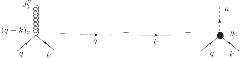
Figure 1: Generalized Ward-Takahashi identity with the NG boson. The straight line indicates the fermion propagator, and the coil-shaped line shows the current $J_{a}^{\mu}$. The dashed line indicates the NG boson propagator. The fermion-NG boson coupling (matrix) is denoted as $g_{c}$.

III Ward-Takahashi identity with NG Bosons

III.1 Modified Ward-Takahashi Identity

We have conserved currents $J^{\mu}_{a}$ with $\partial_{\mu}J^{\mu}_{a}=0$ when $\mathcal{L}$ is invariant under some transformation. When the symmetry is spontaneously broken, non-vanishing $\partial_{\mu}J^{\mu}_{a}$ represents the Nambu-Goldstone boson. For the transformation $\psi\rightarrow\psi-i\theta T_{a}\psi$, the current is

$$J_{a}^{\mu}=\psi^{{\dagger}}\Gamma^{\mu}T_{a}\psi.$$ (103)

Let us examine the expectation value $\langle T(J^{\mu}_{a}(x)\psi(y)\psi^{{\dagger}}(z))\rangle$ where $x$ indicates the four vector $x=(x^{0},{\bf r})$. We evaluate the derivative of this expectation value:

$$\partial_{\mu}^{x}\langle T(J^{\mu}_{a}(x)\psi(y)\psi^{{\dagger}}(z))\rangle=\langle T(\partial_{\mu}^{x}J_{a}^{\mu}(x)\psi(y)\psi^{{\dagger}}(z))\rangle$$

$$~{}~{}~{}+\delta(x^{0}-y^{0})\langle T([J_{a}^{0}(x),\psi(y)]\psi^{{\dagger}}(z))\rangle$$

$$~{}~{}~{}+\delta(x^{0}-z^{0})\langle T(\psi(y)[J_{a}^{0}(x),\psi^{{\dagger}}(z)])\rangle.$$ (104)

We set $\Gamma^{0}=1$ (unit matrix) for simplicity and we have

$$J_{a}^{0}=\psi^{{\dagger}}T_{a}\psi,~{}~{}~{}Q_{a}=\int d{\bf r}J_{a}^{0}.$$ (105)

We use the commutation relations:

$$\delta(x^{0}-y^{0})[J_{a}^{0}(x),\psi(y)] = -\delta(x-y)T_{a}\psi(x)$$ (106)

$$\delta(x^{0}-y^{0})[J_{a}^{0}(x),\psi^{{\dagger}}(y)] = \delta(x-y)\psi^{{\dagger}}(x)T_{a}.$$ (107)

This results in the following equation,

$$\partial_{\mu}^{x}\langle T(J^{\mu}_{a}(x)\psi(y)\psi^{{\dagger}}(z))\rangle=\lambda\langle T(\pi_{a}(x)\psi(y)\psi^{{\dagger}}(z))\rangle$$

$$~{}~{}~{}-\delta(x-y)T_{a}\langle T(\psi(x)\psi^{{\dagger}}(z))\rangle$$

$$+~{}~{}~{}+\delta(x-z)\langle T(\psi(y)\psi^{{\dagger}}(z))\rangle T_{a}.$$ (108)

This is the Ward-Takahashi identity with the Nambu-Goldstone boson.

We define the Fourier transforms of correlation functions. We introduce the vertex function $\Gamma_{a}^{\mu}$:

$$\int d^{4}x\int d^{4}y\int d^{4}ze^{-ip\cdot x-ik\cdot y+iq\cdot z}\partial_{\mu}^{x}\langle TJ_{a}^{\mu}(x)\psi(y)\psi^{{\dagger}}(z)\rangle$$

$$~{}~{}~{}\equiv ip_{\mu}i(2\pi)^{4}\delta^{4}(p+k-q)G(k)\Gamma_{a}^{\mu}(k,q)G(q),$$ (109)

where $G(k)$ is the Green’s function of fermion $\psi$ given by

$$i(2\pi)^{4}\delta^{4}(k-q)G(k)\equiv\int d^{4}y\int d^{4}ze^{-ik\cdot y+iq\cdot z}\langle T(\psi(y)\psi^{{\dagger}}(z))\rangle.$$ (110)

$k$ is the four momentum $k=(k^{0},{\bf k})$. There appears the expectation value $\langle T(\pi_{a}(x)\psi(y)\psi^{{\dagger}}(z))\rangle$ that contains $\pi_{a}$. The interaction between fermions would induce an effective interaction between $\pi_{a}$ and fermions. Thus we introduce the fermion-NG boson coupling (vertex function) $g_{a}(k,q)$:

$$\int d^{4}x\int d^{4}y\int d^{4}ze^{-ip\cdot x-ik\cdot y+iq\cdot z}\langle T(\pi_{a}(x)\psi(y)\psi^{{\dagger}}(z))\rangle$$

$$~{}~{}~{}=(2\pi)^{4}\delta^{4}(p+k-q)\big{[}\sum_{b}f_{amb}G(k)T_{b}G(q)$$

$$~{}~{}~{}+\sum_{c}G(k)g_{c}(k,q)G(q)D_{ca}(q-k)\big{]},$$ (111)

where the summation with respect to $c$ is taken for which $D_{ca}$ does not vanish. Because $\pi_{a}$ is in general a linear combination of $\psi^{{\dagger}}T_{a}\psi$, we can consider $\langle T(\psi^{{\dagger}}(x)T_{a}\psi(x)\psi(y)\psi^{{\dagger}}(z))\rangle$. We define

$$B_{ab}(x-y)=-i\langle T(\psi^{{\dagger}}T_{a}\psi)(x)(\psi^{{\dagger}}T_{b}\psi)(y)\rangle,$$ (112)

and its Fourier transform given as

$$B_{ab}(k)=\int d^{4}xe^{-ik\cdot(x-y)}B_{ab}(x-y).$$ (113)

In the non-interacting case, $B_{ab}(k)$ is

$$B_{ab}^{0}(q)=-i\int\frac{d^{4}k}{(2\pi)^{4}}{\rm Tr}T_{a}G^{0}(k)T_{b}G^{0}(k+q).$$ (114)

Because we have

$$D_{ab}(q)=\sum_{cd}f_{acm}f_{bdm}B_{cd}(q),$$ (115)

we set

$$f_{c}(k,q)=\sum_{a}f_{amc}g_{a}(k,q),$$ (116)

to obtain

$$\int d^{4}xd^{4}yd^{4}ze^{-ip\cdot x-ik\cdot y+iq\cdot z}\langle T(\psi^{{\dagger}}(x)T_{a}\psi(x)\psi(y)\psi^{{\dagger}}(z))\rangle$$

$$~{}~{}=(2\pi)^{4}\delta^{4}(p+k-q)\big{[}-G(k)T_{a}G(q)$$

$$~{}~{}~{}-\sum_{c}G(k)f_{c}(k,q)B_{ca}(q-k)G(q)\big{]}.$$

In the momentum space, the Ward-Takahashi identity is written in the form:

$$(q-k)_{\mu}G(k)\Gamma_{a}^{\mu}(k,q)G(q) = iT_{a}G(q)-iG(k)T_{a}$$

$$-\lambda G(k)\Gamma_{a}(k,q)G(q),$$

where

$$\Gamma_{a}(k,q)=\sum_{c}f_{amc}T_{c}+\sum_{c}g_{c}(k,q)D_{ca}(q-k).$$ (119)

This is diagrammatically shown in Fig.1 and is written as

$$(q-k)_{\mu}\Gamma_{a}^{\mu}(k,q)=iG^{-1}(k)T_{a}-iT_{a}G^{-1}(q)-\lambda\Gamma_{a}(k,q).$$ (120)

This is the modified Ward-Takahashi identity with the correction from the Nambu-Goldstone boson. We have let that $M=T_{m}\in\{T_{c}\}$. Because $\lambda D_{ab}(q-k\rightarrow 0)=\sum_{c}f_{amc}f_{bmc}\Delta$ as $\lambda\rightarrow 0$, we obtain

$$\lambda\Gamma_{a}(k,k)\rightarrow\sum_{cd}g_{c}(k,k)f_{cmd}f_{amd}\Delta,$$ (121)

as $\lambda\rightarrow 0$. Then we have the relation

$$iG^{-1}(k)T_{a}-iT_{a}G^{-1}(k)-\Delta\sum_{c}g_{c}(k,k)\alpha_{ca}=0,$$ (122)

with $\alpha_{ca}=\sum_{d}f_{amd}f_{cmd}$. The Green’s function $G(k)$ is expressed as

$$G^{-1}(k)=k_{0}-{\bf\Gamma}\cdot{\bf k}-\Sigma(k),$$ (123)

where we put $\Gamma^{\mu}=(\Gamma^{0}=1,{\bf\Gamma})$, and the above relation results in

$$iT_{a}\Sigma(k)-i\Sigma(k)T_{a}+\Delta\sum_{c}g_{c}(k,k)\alpha_{ca}=0.$$ (124)

When the interaction term is explicitly given, the self-energy $\Sigma(k)$ and the vertex $\Gamma_{a}$ can be calculated. This relation gives the equation for the order parameter $\Delta$ and the coupling constant $g_{c}$.

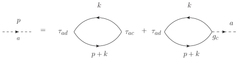
Figure 2: Equation for the NG boson Green’s function. The solid line indicates the fermion propagator, and the dashed line shows the NG boson propagator. $\tau_{ad}$ indicates $\tau_{ad}=\sum_{d}f_{amd}T_{d}$.

III.2 Vertex Function for NG boson Green’s Functions

Let us investigate the equations for Nambu-Goldstone Green’s functions. First note that $\pi_{a}=i\psi^{{\dagger}}[T_{a},T_{m}]\psi=-\sum_{c}f_{amc}\psi^{{\dagger}}T_{c}\psi$. From Eq.(111), we have

$$\langle T\pi_{a}(x)\psi(y)\psi^{{\dagger}}(z)\rangle$$

$$= \int\frac{d^{4}p}{(2\pi)^{4}}\frac{d^{4}k}{(2\pi)^{4}}e^{ip\cdot x+ik\cdot y-i(p+k)\cdot z}$$

$$\times\Big{[}\sum_{c}f_{amc}G(k)T_{c}G(p+k)$$

$$+\sum_{c}G(k)g_{c}(k,k+p)D_{ca}(p)G(k+p)\Big{]}.$$

This indicates

$${\rm Tr}\sum_{c}f_{amc}T_{c}\langle T\pi_{a}(x)\psi(y)\psi^{{\dagger}}(y_{0}+\delta,{\bf y})\rangle$$ (126)

$$= -\sum_{c}f_{amc}\langle T\pi_{a}(x)\psi^{{\dagger}}(y_{0}+\delta,{\bf y})T_{c}\psi(y)\rangle$$

$$= \langle T\pi_{a}(x)\pi_{a}(y)\rangle,$$

where we use ${\rm Tr}T_{c}\pi_{a}(x)\psi(y)\psi^{{\dagger}}(y)={\rm Tr}\pi_{a}(x)T_{c}\psi(y)\psi^{{\dagger}}(y)=-\pi_{a}(x)\psi^{{\dagger}}(y)T_{c}\psi(y)$ because $\pi_{a}(x)$ is an operator (not a matrix). Then the NG boson Green’s function is given by

$$\langle T\pi_{a}(x)\pi_{a}(y)\rangle$$ (127)

$$= \int\frac{d^{4}p}{(2\pi)^{4}}\int\frac{d^{4}k}{(2\pi)^{4}}e^{ip\cdot(x-y)}{\rm Tr}\sum_{d}f_{amd}T_{d}$$

$$\times\Big{[}\sum_{c}f_{amc}G(k)T_{c}G(p+k)$$

$$+\sum_{c}G(k)g_{c}(k,k+p)D_{ca}(p)G(k+p)\Big{]}.$$

This reads

$$D_{aa}(p) = -i{\rm Tr}\sum_{cd}\int\frac{d^{4}k}{(2\pi)^{4}}\Big{[}f_{amd}f_{amc}T_{d}G(k)T_{c}G(k+p)$$ (128)

$$+ f_{amd}T_{d}G(k)g_{c}(k,k+p)G(k+p)D_{ca}(p)\Big{]}.$$

This is shown diagrammatically in Fig.2. The Green’s function for different NG bosons $\pi_{a}$ and $\pi_{b}$ is

$$D_{ab}(p) = -i{\rm Tr}\sum_{cd}\int\frac{d^{4}k}{(2\pi)^{4}}\Big{[}f_{bmd}f_{amc}T_{d}G(k)T_{c}G(k+p)$$ (129)

$$+ f_{bmd}T_{d}G(k)g_{c}(k,k+p)G(k+p)D_{ca}(p)\Big{]}.$$

When $\sum_{c}f_{amc}f_{bmc}=0$ for $a\neq b$, we neglect $D_{ab}$ ($a\neq b$) because $D_{ab}(p)\rightarrow 0$ as $p\rightarrow 0$. In this case, the equation for $D_{aa}(p)$ reads

$$D_{aa}(p) = \Big{[}1+i{\rm Tr}\int\frac{d^{4}k}{(2\pi)^{4}}\sum_{d}f_{amd}T_{d}G(k)$$

$$\times g_{a}(k,k+p)G(k+p)\Big{]}^{-1}$$

$$\times (-i){\rm Tr}\sum_{cd}\int\frac{d^{4}k}{(2\pi)^{4}}f_{amd}f_{amc}T_{d}G(k)T_{c}G(k+p).$$

$g_{a}(k.k+p)$ should be determined on the basis of the Ward-Takahashi identity.

III.3 Higgs boson

We define the Higgs field $h(x)$ by

$$h(x)=\psi^{{\dagger}}(x)T_{m}\psi(x),$$ (131)

where $T_{m}$ is the basis corresponding to broken symmetry. The Higgs boson indicates the fluctuation of the amplitude of the order parameter $\Delta=\langle\psi^{{\dagger}}T_{m}\psi\rangle$. Thus, in a strict sense, the Higgs field should be defined as

$$\delta h(x)=\psi^{{\dagger}}(x)T_{m}\psi(x)-\Delta.$$ (132)

We simply call the field $h(x)$ the Higgs field. $h(x)$ is composed of fermions as in the case of NG bosons. Thus the Green’s function of the Higgs boson,

$$H(x-y) = -i\langle T(h(x)h(y))\rangle$$ (133)

$$= \int\frac{d^{4}p}{(2\pi)^{4}}e^{ip\cdot(x-y)}H(p),$$

is also evaluated in a similar way to that of Nambu-Goldstone bosons. We introduce the vertex function $g_{H}(k,k+p)$ to write

$$H(p) = -i{\rm Tr}\int\frac{d^{4}k}{(2\pi)^{4}}\Big{[}T_{m}G(k)T_{m}G(k+p)$$ (134)

$$+ T_{m}G(k)g_{H}(k,k+p)G(k+p)H(p)\Big{]}.$$

The vertex function $g_{H}(k,k+p)$ will depend on the interaction between electrons. It is reasonable to assume that $g_{H}(k,k+p)$ is proportional to $T_{m}$ since $h(x)=\psi^{{\dagger}}T_{m}\psi$. Thus we denote $g_{H}(k,k+p)=g_{m}(k,k+p)$. The dispersion of the Higgs boson is determined by this equation.

III.4 NG Boson-NG boson and NG Boson-Higgs Boson Couplings

Because we have the NG boson-fermion coupling and the Higgs-fermion coupling, there are NG boson-NG boson coupling and NG boson-Higgs coupling as effective interactions. The figures 3(a) and 3(b) indicate couplings of two and three particles, respectively. Multi-particle couplings also possibly exist. When the Lagrangian including the interaction term is given, we can evaluate multi-particle vertex functions using some calculation methods.

The figure 3(a) shows NG boson-NG boson coupling or NG boson-Higgs boson coupling. In general, the NG boson-Higgs boson coupling $\pi_{a}h$ vanishes because of the orthogonality of bases $T_{a}$: ${\rm Tr}T_{a}T_{b}=c\delta_{ab}$.

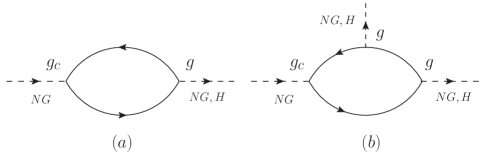
Figure 3: NG boson-NG boson (or Higgs boson) couplings. The solid line indicates the fermion propagator, and the dashed line shows the NG boson or the Higgs boson propagator. (b) shows the coupling such as $\pi_{a}\pi_{b}h$. $g_{c}$ and $g$ indicate the vertex functions where $g=g_{d}$ or $g=g_{H}$.

III.5 Some Physical Systems

III.5.1 Ferromagnetic transition

We take $G=SU(2)$ and a fermion doublet $\psi=^{t}(\psi_{\uparrow},\psi_{\downarrow})$. Let us consider the Hubbard modelhub63 ; yam98 ; yan01 ; yan16b

$$\mathcal{L}=i\psi^{{\dagger}}\partial_{t}\psi-\psi^{{\dagger}}\xi(\nabla)\psi-U\psi^{{\dagger}}_{\uparrow}(x)\psi_{\uparrow}(x)\psi^{{\dagger}}_{\downarrow}(x)\psi_{\downarrow}(x),$$ (135)

where $\xi(\nabla)=\epsilon(\nabla)-\mu$ is the electron dispersion relation with chemical potential $\mu$ and last term indicates the repulsive interaction ($U>0$). The bases $\{T_{a}\}$ are given by Pauli matrices: $T_{a}=\sigma_{a}$ ($a=$ 1, 2 and 3). The structure constants are $f_{abc}=2\epsilon_{abc}$. This Lagrangian is invariant under the transformations

$$\psi\rightarrow e^{-i\theta\sigma_{a}}\psi,~{}~{}~{}(a=1,2,3).$$ (136)

The symmetry breaking term is given by the magnetization of electrons for a ferromagnetic transition:

$$\mathcal{L}_{SB}=\lambda\psi^{{\dagger}}\sigma_{3}\psi=\lambda(\psi^{{\dagger}}_{\uparrow}\psi_{\uparrow}-\psi^{{\dagger}}_{\downarrow}\psi_{\downarrow}).$$ (137)

This term breaks the symmetry $\psi\rightarrow e^{-i\theta\sigma_{a}}\psi$ for $a=1$, 2. The corresponding Nambu-Goldstone bosons are

$$\pi_{1} = i\psi^{{\dagger}}[\sigma_{1},\sigma_{3}]\psi=2\psi^{{\dagger}}\sigma_{2}\psi,$$

$$\pi_{2} = i\psi^{{\dagger}}[\sigma_{2},\sigma_{3}]\psi=-2\psi^{{\dagger}}\sigma_{1}\psi.$$ (138)

The excitation mode represented by $\pi_{1}$ and $\pi_{2}$ is spin-flip process, that is, the spin-wave excitation. We make a linear combination of $\pi_{1}$ and $\pi_{2}$ as $\pi\equiv(i\pi_{1}-\pi_{2})/4=\psi^{{\dagger}}_{\uparrow}\psi_{\downarrow}$ and $\pi^{{\dagger}}=(-i\pi_{1}-\pi_{2})/4=\psi^{{\dagger}}_{\downarrow}\psi_{\uparrow}$. Actually, there is only one Nambu-Goldstone boson $\pi$ in a ferromagnetic state. This is consistent with the general theory for counting the number of NG bosonswat12 ; hid13 and also with the vanishing theorem. As shown in the section II, $\pi$ represents a massless excitation.

The electron Green’s function is given in the form:

$$G=\left(\begin{array}[]{cc}G_{\uparrow\uparrow}&0\\ 0&G_{\downarrow\downarrow}\\ \end{array}\right),$$ (141)

where

$$G_{\sigma\sigma}(x-y)=-i\langle T\psi_{\sigma}(x)\psi^{{\dagger}}_{\sigma}(y)\rangle.$$ (142)

The self-energy $\Sigma$ is similarly defined as

$$\Sigma=\left(\begin{array}[]{cc}\Sigma_{\uparrow}&0\\ 0&\Sigma_{\downarrow}\\ \end{array}\right),$$ (145)

where $G_{\sigma\sigma}^{-1}(k)=k_{0}-\xi({\bf k})-\Sigma_{\sigma}$. From the Ward-Takahashi identity in Eq.(122), we obtain

$$iG^{-1}\sigma_{1}-i\sigma_{1}G^{-1}-\Delta g_{1}f_{123}^{2} = 0,$$ (146)

$$iG^{-1}\sigma_{2}-i\sigma_{2}G^{-1}-\Delta g_{2}f_{123}^{2} = 0.$$ (147)

We set $g_{a}=\sum_{c}\epsilon_{acm}\sigma_{c}\tilde{g}$ such as $g_{1}=\sigma_{2}\tilde{g}$ and $g_{2}=-\sigma_{1}\tilde{g}$. Making a linear combination $\sigma_{2}-i\sigma_{1}$, the above relation results in

$$\Sigma_{\downarrow}(k)-\Sigma_{\uparrow}(k)=\Delta f_{123}^{2}\tilde{g}(k,k).$$ (148)

This is the relation between the electron-NG boson coupling and the self-energy. When the self-energy is evaluated, the coupling constant $\tilde{g}$ is determined from this relation. This relation can be also regarded as the gap equation for $\Delta$.

Because $\pi=i(\pi_{1}+i\pi_{2})/4$, the correlation function in Eq.(111) leads to

$$\int d^{4}x\int d^{4}y\int d^{4}ze^{-ip\cdot x-ik\cdot y+iq\cdot z}\langle T(\pi(x)\psi(y)\psi^{{\dagger}}(z))\rangle$$

$$~{}~{}~{}=(2\pi)^{4}\delta^{4}(p+k-q)\Big{[}-G(k)\left(\begin{array}[]{cc}0&1\\ 0&0\\ \end{array}\right)G(q)$$ (151)

$$~{}~{}~{}-4G(k)\left(\begin{array}[]{cc}0&1\\ 0&0\\ \end{array}\right)G(q)\tilde{g}(k,q)\tilde{D}(q-k)\Big{]},$$ (154)

where $\tilde{D}(k)$ is the Fourier transform of the Green’s function of $\pi$:

$$\tilde{D}(x-y)=-i\langle T\pi(x)\pi^{{\dagger}}(y)\rangle.$$ (155)

Here we used the relation $\tilde{D}=D_{11}/8=D_{22}/8$. When we calculate the Green’s function $\langle T(\pi(x)\psi(y)\psi^{{\dagger}}(z))\rangle$ by means of the perturbation in Coulomb interaction $U$, the correction of the order of $U$ is

$$-G(k)\left(\begin{array}[]{cc}0&1\\ 0&0\\ \end{array}\right)G(q)-UG(k)\left(\begin{array}[]{cc}0&1\\ 0&0\\ \end{array}\right)G(q)\tilde{D}(q-k),$$ (160)

in the momentum space. This gives

$$\tilde{g}(k,q)=\frac{U}{4}+\cdots.$$ (162)

This is consistent with the self-energy-coupling relation in Eq.(148) since the self-energy is given by $\Sigma_{\sigma}=Un_{-\sigma}+\cdots$ where $n_{\sigma}$ is the density of electrons with spin $\sigma$, and we have $\Delta=n_{\uparrow}-n_{\downarrow}$.

III.5.2 Superconductivity

We obtain the Ward-Takahashi identity for superconductors in a similar waykoy14 ; koy16 . The Higgs field $h$ is defined as

$$h=\psi^{{\dagger}}\sigma_{1}\psi=\psi^{{\dagger}}_{\uparrow}\psi^{{\dagger}}_{\downarrow}+\psi_{\downarrow}\psi_{\uparrow}.$$ (163)

Near the critical temperature, the effective action for $h$ is given by the time-dependent Ginzburg-Landau (TDGL) action with the dissipation effect. The Higgs mode in a superconductor is clearly defined at low temperatures ($T\ll T_{c}$). The Higgs Green’s function is given by

$$P_{11}(\omega,{\bf q})\equiv-i\frac{1}{2}{\rm Tr}\sigma_{1}G_{0}(\epsilon,{\bf k})\sigma_{1}G_{0}(\epsilon+\omega,{\bf k}+{\bf q}),$$ (164)

where $G_{0}$ is the electron Green’s function:

$$G_{0}^{-1}(\epsilon,{\bf k})=\left(\begin{array}[]{cc}\epsilon-\xi({\bf k})&-\Delta\\ -\Delta&\epsilon+\xi({\bf k})\\ \end{array}\right),$$ (167)

where $\Delta$ is assumed to be real. $1/g+P_{11}(\omega,{\bf q}=0)$ has a zero at $\omega=2\Delta$koy16 . At absolute zero, for small $\omega$ and $q=|{\bf q}|$, we obtain

$$\frac{1}{g}+P_{11}(\omega,{\bf q})=N(0)\Big{[}1-\frac{1}{3}\left(\frac{\omega}{2\Delta}\right)^{2}\Big{]}+N(0)\frac{1}{3}c_{s}^{2}\left(\frac{q}{2\Delta}\right)^{2},$$ (168)

where we adopt the approximation that the density of states is constant and we used the gap equation,

$$\frac{1}{g}=N(0)\int d\xi\frac{1}{2E(\xi)}.$$ (169)

We put $c_{s}^{2}=v_{F}^{2}/3$.

The relativistic model of superconductivity is given by the Nambu-Jona-Lasinio modelnam61 :

$$\mathcal{L}=\bar{\psi}i\gamma^{\mu}\partial_{\mu}\psi+g_{NJL}[(\bar{\psi}\psi)^{2}-(\bar{\psi}\gamma_{5}\psi)^{2}].$$ (170)

This Lagrangian is invariant under the particle number and Chiral transformations:

$$\psi\rightarrow e^{i\theta}\psi,~{}~{}\bar{\psi}\rightarrow\bar{\psi}e^{-i\theta}$$ (171)

$$\psi\rightarrow e^{i\gamma_{5}\theta}\psi,~{}~{}\bar{\psi}\rightarrow\bar{\psi}e^{i\gamma_{5}\theta}.$$ (172)

The symmetry breaking term is

$$\mathcal{L}_{SB}=\lambda\bar{\psi}\psi,$$ (173)

with $M=\gamma_{0}$. Then the invariance under the transformation $\psi\rightarrow\exp(i\gamma_{5}\theta)\psi$ is violated, and it is clear from our general theory that the NG boson and Higgs boson are given by

$$\pi=i\bar{\psi}\gamma_{5}\psi,~{}~{}~{}h=\bar{\psi}\psi.$$ (174)

IV Summary

We have given a formulation of the Nambu-Goldstone boson in fermion and boson systems with spontaneous symmetry breaking. The Nambu-Goldstone bosons are determined when the order parameter in the phase transition is given in a system with a continuous symmetry. The Nambu-Goldstone boson $\pi_{a}$ is explicitly given by the formula $\pi_{a}=i\psi^{{\dagger}}[T_{a},T_{m}]\psi$ for a fermion field $\psi$ where $T_{a}$ and $T_{m}$ are elements of basis set of the Lie algebra, where $T_{m}$ corresponds to the broken symmetry. We have given a proof that $\pi_{a}$ is a boson with vanishing mass by showing that the susceptibility $\chi_{\Delta}$ is proportional to the NG boson Green’s function at $\omega=0$ and ${\bf q}=0$: $\chi_{\Delta}\propto D_{aa}(\omega=0,{\bf q}=0)$.

When $\sum_{c}f_{amc}f_{bmc}=0$ holds, the vanishing property holds where the Green’s function $D_{ab}(q)$ of $\pi_{a}$ and $\pi_{b}$, given by the Fourier transform of $\langle T\pi_{a}(x)\pi_{b}(y)\rangle$, vanishes in the limit $q\rightarrow 0$: $D_{ab}(q=0)=0$. This means that two bosons $\pi_{a}$ and $\pi_{b}$ are not independent and there is a constraint.

The Ward-Takahashi identity is generalized in the presence of spontaneous symmetry breaking. The violation of the conservation of the current is compensated by the inclusion of a contribution from the Nambu-Goldstone boson. We introduced the NG boson-fermion vertex function in the Ward-Takahashi identity. With this vertex function, the equation for NG boson Green’s functions is closed. The NG boson-NG boson couplings and NG boson-Higgs boson couplings are also introduced due to the NG boson-fermion and Higgs boson-fermion vertex functions.

The Nambu-Goldstone boson degrees of freedom lead to the effective Lagrangian. They describe the spin wave in magnetic systemskit87 ; tsv03 and the effective model is in general given by the non-linear sigma modeltsv03 ; leu94 ; leu94b . In superconductors, the effective action is given by the sine-Gordon modelkoy96 ; yan12 ; yan13 ; nit15 ; yan16 . We expect that the coupling between NG bosons and fermions can be determined on the basis of the Ward-Takahashi identity.

References

- (1) J. Goldstone, Nuovo Cimento 9, 154 (1961).
- (2) Y. Nambu, Phys. Rev. Lett. 4, 380 (1960).
- (3) J. Goldstone, A. Salam and S. Weinberg, Phys. Rev. 127, 965 (1962).
- (4) S. Weinberg, The Quantum Theory of Fields Vol. II, Cambridge University Press, Cambridge, 1995).
- (5) S. Coleman, Aspects of Symmetry (Cambridge University Press, Cambridge, 1985).
- (6) Y. Nambu and G. Jona-Lasinio, Phys. Rev. 122, 345 (1961).
- (7) P. W. Higgs, Phys. Rev. Lett. 13, 508 (1964).
- (8) S. Weinberg, Phys. Rev. Lett. 29, 1698 (1972).
- (9) M. L. Goldberger and S. Treiman, Phys. Rev. 111, 354 (1966).
- (10) T. Brauner, Symmetry 2, 609 (2010).
- (11) H. B. Nielsen and S. Chadha, Nucl. Phys. B105, 445 (1976).
- (12) H. Watanabe abd T. Brauner, Phys. Rev. D84, 125013 (2011): 85, 085010 (2012).
- (13) H. Watanabe and H. Murayama, Phys. Rev. Lett. 108, 251602 (2012).
- (14) Y. Hidaka, Phys. Rev. Lett. 110, 091601 (2013).
- (15) K. Odagiri and T. Yanagisawa, Eur. Phys. J C73, 2525 (2013).
- (16) H. Watanabe and H. Murayama, Phys. Rev. D90, 121703 (2014).
- (17) M. Nitta and D. A. Takahashi, Phys. Rev. D91, 025018 (2015).
- (18) P. W. Anderson, Basic Notions of Condensed Matter Physics (Benjamin/Cummings Publishing Company, London, 1984).
- (19) V. L. Ginzburg and L. D. Landau, Zh. Eksp. Teor. Fiz. 20, 1064 (1950).
- (20) J. Bardeen, L. N. Cooper and J. R. Schrieffer, Phys. Rev. 108, 1175 (1957).
- (21) A. A. Abrikosov, Fundamentals of the Theory of Metals (North-Holland, Amsterdam, 1988).
- (22) R. M. White, Quantum Theory of Magnetism (Springer-Verlag, Berlin, 2006).
- (23) L. Leplae, H. Umezawa and F. Mancini, Phys. Rep. 10, 151 (1974).
- (24) J. C. Ward, Phys. Rev. 78, 182 (1950).
- (25) Y. Takahashi, Nuovo Cimento, 6, 371 (1957).
- (26) V. N. Gribov, Phys. Lett. B336, 243 (1994).
- (27) L. H. Ryder, Quantum Field Theory (Cambridge University Press, Cambridge, 1996).
- (28) H. Georgi, Lie Algebras in Particle Physics (Westview Press, New York, 1999).
- (29) A. A. Abrikosov, L. P. Gor’kov and I. Ye. Dzyaloshinskii, Quantum Field Theoretical Methods in Statistical Physics (Pergamon Press, Oxford, 1965; Dover Publication, New York, 1975).
- (30) A. L. Fetter and J. D. Walecka, Quantum Theory of Many-Particle Systems (MacGraw-Hill Book Company, New York, 1971; Dover Publication, New York, 2003).
- (31) T. Moriya, Spin Fluctuations in Itinerant Electron Mgnetism (Springer-Verlag, Berlin, 1985).
- (32) J. Hubbard, Proc. Roy. Soc. London 276, 238 (1963).
- (33) K. Yamaji, T. Yanagisawa, T. Nakanishi and S. Koike, Physica C304, 225 (1998).
- (34) T. Yanagisawa, S. Koike and K. Yamaji, Phys. Rev. B64, 184509 (2001); ibid, B67, 132408 (2003).
- (35) T. Yanagisawa, J. Phys. Soc. Jpn. 85, 114707 (2016).
- (36) T. Koyama, J. Phys. Soc. Jpn. 83, 074715 (2014).
- (37) T. Koyama, J. Phys. Soc. Jpn. 85, 064715 (2016).
- (38) C. Kittel, Quantum Theory of Solids (John Wiley and Sons, Inc., New York, 1987).
- (39) A. M. Tsvelik, Quantum Field Theory in Condensed Matter Physics (Cambridge University Press, Cambridge, 2003).
- (40) H. Leutwyler, Phys. Rev. D49, 3033 (1994).
- (41) H. Leutwyler, Ann. Phys. 235, 165 (1994).
- (42) T. Koyama and M. Tachiki, Phys. Rev. B54, 16183 (1996).
- (43) T. Yanagisawa, Y. Tanaka, I. Hase and K. Yamaji, J. Phys. Soc. Jpn. 81, 024712 (2012).
- (44) T. Yanagisawa and I. Hase, J. Phys. Soc. Jpn. 82, 124704 (2013).
- (45) M. Nitta, Nucl. Phys. B895, 288 (2015).
- (46) T. Yanagisawa, EPL 113, 41001 (2016).