Analytic treatment of the thermoelectric properties for two coupled quantum dots threaded by magnetic fields

Abstract

Coupled double quantum dots (c-2QD) connected to leads have been widely adopted as prototype model systems to verify interference effects on quantum transport at the nanoscale. We provide here an analytic study of the thermoelectric properties of c-2QD systems pierced by a uniform magnetic field. Fully analytic and easy-to-use expressions are derived for all the kinetic functionals of interest. Within the Green^′s function formalism, our results allow a simple inexpensive procedure for the theoretical description of the thermoelectric phenomena for different chemical potentials and temperatures of the reservoirs, different threading magnetic fluxes, dot energies and interdot interactions; moreover they provide an intuitive guide to parametrize the system Hamiltonian for the design of best performing realistic devices. We have found that the thermopower $S$ can be enhanced by more than ten times and the figure of merit $ZT$ by more than hundred times by the presence of a threading magnetic field. Most important, we show that the magnetic flux increases also the performance of the device under maximum power output conditions.

I INTRODUCTION

Quantum dot systems have attracted enormous interest as workable thermoelectric device candidates for the study of electronic and thermal quantum transport at the nanoscale. The origin of such an interest both from the theoretical and the experimental side, resides in the potential they offer, as artificial nanoscale junctions, to explore a large variety of thermoelectric effects. Relevance of nanostructures as performing energy harvesting devices was envisaged in the pioneering paper of Hick and DresselhausDRESS93 . Since then nanoscale thermoelectricity has been addressed by an increasing number of theoretical and experimental works; a perspective of the field can be found in the focus point collection in Ref.[SANCEZ14, ]. In particular, interference Ahronov-BohmBROGI15 ; KANG04 ; KUBA02 ; FAZIO11 , Fano ORELLANA03 ; SILVA12 ; WIERB11 ; GARCIA13 , Dicke WANG13 ; ORELLANA94 and Mach-Zehnder HOFER15 ; Samuelson17 effects, inter- and intra-dot correlation effectsBULKA04 ; SIERRA16 , coherent transport modification by external magnetic fields and gate voltages.BAI04 ; LIU10 ; PYL10 , have been exploited to control the performance of thermoelectric heat devices.

The system composed by two single-level quantum dots coupled to each other (c-2QD) via metallic leads, in two terminal or multiterminal setups RSAN15 , and via an interdot tunneling are most appropriate to probe how the Hamiltonian system parameters and external conditions can be varied to optimize the energy conversion efficiency and the output power of the thermoelectric device. This is a demanding task because such parameters often play conflicting roles in the optimization process. Strategies for increasing thermoelectric performances utilizing a steep slope in the transmission function ${\mathcal{T}}$(E), or its specific shape, or its resonances, have been well described in Ref.[Lambert16, ] where also a comparison between the thermoelectric efficiency of inorganic and organic materials is discussed.

Enhancing thermoelectric performance in linear regimes, requires maximization of the dimensionless thermoelectric figure of merit $ZT=\sigma S^{2}T/\kappa$ where $\sigma$ is the electrical conductance, $S$ the thermopower (Seebeck) coefficient, $T$ is the temperature and $\kappa=\kappa_{e}+\kappa_{p}$ is the thermal conductance (which includes electronic and lattice contributions). In the search of optimal thermoelectric response of the device, most important quantities are its maximum efficiency as thermoelectric generator, and the efficiency at the maximum of the output power.

A crucial aspect for the evaluation of the thermoelectric response of a device, is the wide parameters range to be explored simultaneously to determine its optimal functioning. In this context, the possibility of using analytic expressions for all the involved thermoelectric functions greatly simplifies the task. In the literature, the analytic treatment of the c-2QD is confined at sufficiently small temperatures by means of the Sommerfeld expansion, extended when necessary to fourth order in $k_{B}T$ in the evaluation of kinetic parameters.SILVA12 In the case of Lorentzian shape of the transmission function, analytic expressions of the thermoelectric transport coefficients have been obtained in terms of digamma functions SANCEZ15 . In the more complicated transmission function of coupled double dot, we provide, in terms of trigamma functions, analytic expressions for the relevant quantities describing the thermoelectric behavior of a c-2QD. The description of the c-2QD electronic transport is performed within the Green^′s function framework. The pole structure of the transmission function ${\mathcal{T}}$(E) is discussed, and the analytic expressions of the kinetic parameters, produced by ${\mathcal{T}}$(E), are obtained in terms of the Bernoulli numbers and of the trigamma function GRAD ; ABRA routinely contained in common software libraries. We have exploited such expressions to study the variation of Seebeck coefficient, figure of merit, energy conversion efficiency and output power, as function of temperatures and chemical potentials of the reservoirs, and of the magnetic field threading the c-2QD. In particular we focus on the thermoelectric efficiency of the c-2QD device, in contact with left and right reservoirs, when it operates at maximum output power conditions.

We adopt the convention that the left reservoir is the hotter one ($T_{L}>T_{R}$) while no a priori assumption is done on the relative position of the chemical potentials $\mu_{L}$ and $\mu_{R}$ of the left and right reservoirs. We consider a two-terminal quantum dot setup, stationary transport conditions, absence of lattice contributions to thermal conductivity ($k\approx k_{e}$), and no electronic correlation effects. The general expression for thermoelectric transport charge current $I$ through the c-2QD, in stationary conditions, is given by BUT90

$$I=\frac{-e}{h}\int_{-\infty}^{+\infty}dE\,{\mathcal{T}}(E)\left[f_{L}(E)-f_{R}(E)\right]$$ (1)

where $f_{L,R}$ denote the Fermi functions of the two reservoirs. The electric power output (${\mathcal{P}}$(E) $>$ 0) is given by

$${\mathcal{P}}=-I\Delta V=\frac{1}{h}\,(\mu_{R}-\mu_{L})\int dE\,{\mathcal{T}}(E)\left[f_{L}(E)-f_{R}(E)\right]\ .$$ (2)

where $\Delta V=(\mu_{L}-\mu_{R})/(-e)$ is the voltage drop and $e=|e|$ is absolute value of the electron charge.

The thermoelectric efficiency of the device is given by the ratio between the work done and the heat extracted from the high temperature reservoir:

$$\eta=\dfrac{W}{Q_{L}}=\dfrac{(Q_{L}-Q_{R})}{Q_{L}}\ .$$ (3)

In steady state conditions the heats per unit time are the thermal currents and $W$ per unit time is the output power ${\mathcal{P}}$. Then

$$\eta=(\mu_{R}-\mu_{L})\frac{\int dE\,{\mathcal{T}}(E)\left[f_{L}(E)-f_{R}(E)\right]}{\int dE(E-\mu_{L})\,{\mathcal{T}}(E)\left[f_{L}(E)-f_{R}(E)\right]}\ .$$ (4)

Expressions from (1) to (4) depend on the thermodynamic parameters $\mu_{L},T_{L},\mu_{R},T_{R}$ and by the c-2QD transmission function ${\mathcal{T}}$(E), and hold in the linear and nonlinear regimes. In this paper we are interested in the linear response of the system so that $\Delta\mu=\mu_{L}-\mu_{R}$ and $\Delta T=T_{L}-T_{R}$ are infinitesimal quantities. To first order in $\Delta T$ and $\Delta\mu$, we can write

$$f_{L}(E)-f_{R}(E)=(-\dfrac{\partial f_{L}}{\partial E})\left[\Delta\mu\ +\ (E-\mu_{L})\,\dfrac{\Delta T}{T_{L}}\right]\ .$$

Expressions (1), (2) and (4) become NOI

$$I_{e} = \frac{-e}{h}\int dE\,{\mathcal{T}}(E)\,(-\frac{\partial f}{\partial E})\left[-e\,\Delta V+(E-\mu)\dfrac{\Delta T}{T}\right]$$ (5a)

$${\mathcal{P}} = \frac{1}{h}\,e\,\Delta V\int dE\,{\mathcal{T}}(E)\,(-\frac{\partial f}{\partial E})\left[-e\,\Delta V+(E-\mu)\frac{\Delta T}{T}\right]$$ (5b)

$$\eta = e\,\Delta V\frac{\int dE\,{\mathcal{T}}(E)\,(-\dfrac{\partial f}{\partial E})\left[-e\,\Delta V+(E-\mu)\dfrac{\Delta T}{T}\right]}{\int dE\,(E-\mu)\,{\mathcal{T}}(E)\,(-\dfrac{\partial f}{\partial E})\left[-e\,\Delta V+(E-\mu)\dfrac{\Delta T}{T}\right]}\,.$$ (5c)

For convenience, in Eqs.(5) the thermodynamic parameters $\mu_{L}$, $T_{L}$ and the Fermi function $f_{L}$ are denoted dropping the now inessential subscript $L$.

In Section II we report details on the c-2QD system and its description in terms of localized functions. In Section III we provide our novel analytic expressions of the transport parameters relevant to control and design of the thermoelectric response of the c-2QD, in the linear response regime. Application of the above expressions and discussion of the results are reported in Section IV where contour plots are reported to better evidence the energy and magnetic field values eventually responsible of efficiency at the maximum output power. We have found that the thermopower $S$ may be enhanced by more than ten times and the figure of merit $ZT$ by more than hundred times due to a threading magnetic field. We red look for chemical potential and magnetic flux values which give the maximum output power and demonstrate that the magnetic flux also increases the corresponding efficiency. Section V contains our conclusions.

II System description and model

In this section we establish a localized basis model for the c-2QD electronic system in contact with the left and right reservoirs, in the presence of a threading magnetic field. To keep the model at the essential, we make some simplifications that could be dropped or better analyzed, when necessary.

Consider a double dot electronic system, with a single orbital per dot, described within the one-electron approximation in the tight-binding framework. The one-electron Hamiltonian can be partitioned in the left lead, central device, right lead, and coupling interaction

$$H=H^{(left)}+H^{(dots)}+H^{(right)}+W^{(dots-leads)}\ .$$ (6)

The electronic system is schematically pictured in Fig.1, where the presence of a uniform magnetic field is also considered.

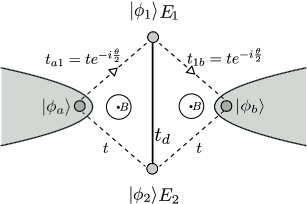
Figure 1: Schematic representation of the double dot electronic system in a symmetric environment for the analysis of thermoelectric properties. In the absence of magnetic field, the four hopping parameters of the ring are equal to $t$ (taken as real). The magnetic field, in the chosen gauge, modifies $t_{a1}\rightarrow te^{-i\theta/2}=t_{1a}^{\ast}$ and $t_{1b}\rightarrow te^{-i\theta/2}=t_{b1}^{\ast}$, where $\theta=2\pi\Phi(B)/\Phi_{0}$, $\Phi(B)$ is the flux of the magnetic field through the entire two-loop ($\phi_{a},\phi_{1},\phi_{b},\phi_{2}$) plaquette, and $\Phi_{0}=hc/e$ is the quantum of flux. In the case of degeneracy $E_{1}=E_{2}=E_{d}$.

The central device, a double dot molecule, is described by the Hamiltonian of the type in the bra-ket notations

$$H^{(dots)}=E_{d}|\phi_{1}\rangle\langle\phi_{1}|+E_{d}|\phi_{2}\rangle\langle\phi_{2}|+t_{d}|\phi_{1}\rangle\langle\phi_{2}|+t_{d}|\phi_{2}\rangle\langle\phi_{1}|\ ,$$ (7)

where $E_{d}$ is the energy of both dots orbitals $\phi_{1},\phi_{2}$, and $t_{d}$ (supposed real and negative) is the off-diagonal coupling between the two dots.

For what concerns the description of two electrodes not yet coupled to the dots, we can proceed as follows. Consider, for instance, the left lead and specifically the “left seed state” $|\phi_{a}>$ that carries the coupling with the central device. The effect of all the other (infinite) degrees of freedom of the left electrode are embodied in the Green’s function $g_{aa}$ on the end seed state. In principle, the Lanczos procedure can be applied to generate the Lanczos chain and, then, to determine the Green’s function [see for instance Ref.[SSP, ]]. The same considerations apply for the right lead. We have

$$g_{aa}^{R}(E)=\langle\phi_{a}|\frac{1}{E-H^{(left)}+i\eta}|\phi_{a}\rangle\quad;\quad g_{bb}^{R}(E)=\langle\phi_{b}|\frac{1}{E-H^{(right)}+i\eta}|\phi_{b}\rangle\ .$$ (8)

Following the routinely adopted “wide-band approximation” we consider explicitly only the imaginary part of the above Green’s functions and disregard the energy dependence. The leads are replaced by the corresponding end states, with the retarded and advanced Green’s functions purely imaginary quantities, independent from energy. In a symmetric geometrical environment, we have

$$g_{aa}^{R}(E)=g_{bb}^{R}(E)\approx-i\pi\rho\quad,\quad g_{aa}^{A}(E)=g_{bb}^{A}(E)\approx+i\pi\rho\qquad(\rho>0)\ ,$$ (9)

where $\rho=-(1/\pi)\,{\rm Im}\,g^{R}$ represents the local density-of-states, assumed to be constant in the typical energy region of actual interest.

The coupling between leads and central device in the absence of magnetic field is represented by a loop with nearest neighbor interaction $t$ (taken as real for simplicity). In the presence of magnetic field, appropriate Peierls phases are introduced. The Berry phases corresponding to the magnetic field are set on the hopping parameters connecting the upper quantum dot $\phi_{1}$ with the end orbitals $\phi_{a},\phi_{b}$ of the electrodes:

$$W^{(dots-leads)} = te^{-i\theta/2)}|\phi_{a}\rangle\langle\phi_{1}|+te^{i\theta/2)}|\phi_{1}\rangle\langle\phi_{a}|+t|\phi_{a}\rangle\langle\phi_{2}|+t|\phi_{2}\rangle\langle\phi_{a}|$$ (10)

$$+ te^{i\theta/2)}|\phi_{b}\rangle\langle\phi_{1}|\,+te^{-i\theta/2)}|\phi_{1}\rangle\langle\phi_{b}|\,+t|\phi_{b}\rangle\langle\phi_{2}|\,+t|\phi_{2}\rangle\langle\phi_{b}|\ .$$

We have now all the ingredients for the calculation of the Green’s function and of the transmission function of the electronic device.

A. Green’s function of the degenerate double dot in magnetic fields

The central part of the device is constituted by the two orbitals of the two quantum dots, coupled one to the other. We can use the renormalization-decimation procedure to fully eliminate the degrees of freedom of the leads, now represented by the end seed states $|\phi_{a}>$ and $|\phi_{b}>$ [see for instance Ref.[SSP, ]]. The retarded self-energies produced by the left lead on the central device become

$$\begin{array}[]{l}\Sigma_{11}^{R(left)}=t_{1a}g_{aa}^{R}t_{a1}=-i\pi\rho\,t^{2}\\[2.84526pt] \Sigma_{12}^{R(left)}=t_{1a}g_{aa}^{R}t_{a2}=-i\pi\rho\,t^{2}e^{i\theta/2}\\[2.84526pt] \Sigma_{21}^{R(left)}=t_{2a}g_{aa}^{R}t_{a1}=-i\pi\rho\,t^{2}e^{-i\theta/2}\\[2.84526pt] \Sigma_{22}^{R(left)}=t_{2a}g_{aa}^{R}t_{a2}=-i\pi\rho\,t^{2}\ .\end{array}$$ (11)

Similar procedures can be followed for the right lead and for the advanced self-energies.

It is convenient to define the real and positive quantity $\gamma/2=\pi\rho\,t^{2}>0$ , that encompasses two parameters of the structure into a single one. Using Eqs.(11), the retarded (advanced) self-energy matrix produced by the left lead in the central device can be cast in the form

$$\Sigma^{R(left)}=-i\,\frac{\gamma}{2}\left[\begin{array}[]{cc}1&e^{i\theta/2}\\[5.69054pt] e^{-i\theta/2}&1\end{array}\right]\quad;\quad\Sigma^{A(left)}=i\,\frac{\gamma}{2}\left[\begin{array}[]{cc}1&e^{i\theta/2}\\[5.69054pt] e^{-i\theta/2}&1\end{array}\right].$$ (12a)

(with $$\gamma>0$$). Similarly, for the retarded and advanced self-energies produced by the right lead, we have

$$\Sigma^{R(right)}=-i\,\frac{\gamma}{2}\left[\begin{array}[]{cc}1&e^{-i\theta/2}\\[5.69054pt] e^{i\theta/2}&1\end{array}\right]\quad;\quad\Sigma^{A(right)}=i\,\frac{\gamma}{2}\left[\begin{array}[]{cc}1&e^{-i\theta/2}\\[5.69054pt] e^{i\theta/2}&1\end{array}\right].$$ (12b)

The total self-energies of the left and right leads are then

$$\Sigma^{R}\!=\!\Sigma^{R(left)}+\Sigma^{R(right)}\!=\!-i\gamma\left[\begin{array}[]{cc}1&\!\!\!\cos(\theta/2)\\[2.84526pt] \cos(\theta/2)&1\end{array}\right]\ \ ,\ \ \Sigma^{A}\!=\!i\gamma\left[\begin{array}[]{cc}1&\!\!\!\cos(\theta/2)\\[2.84526pt] \cos(\theta/2)&1\end{array}\right].$$ (12c)

Finally the coupling parameters are given by the expressions

$$\Gamma^{(left)}\!=\!i[\Sigma^{R(left)}\!-\!\Sigma^{A(left)}]=\gamma\left[\begin{array}[]{cc}1&\!\!\!e^{i\theta/2}\\[5.69054pt] e^{-i\theta/2}&1\end{array}\right]\ ,\ \Gamma^{(right)}=\gamma\left[\begin{array}[]{cc}1&\!\!\!e^{-i\theta/2}\\[5.69054pt] e^{i\theta/2}&1\end{array}\right].$$ (12d)

It should be noticed that the self-energies $\Sigma$ and the broadening parameters $\Gamma$ depend on the applied magnetic field, but are completely independent from the energy variable. This nice feature is a consequence of the wide band approximation and fosters the possibility of a fully analytic treatment of transport parameters, which is a key aspect of this article.

The retarded effective Hamiltonian for the double-dot in the central device, after the full decimation procedure of the leads, is given by the expression

$$H^{R(eff)}=H^{(dots)}+\Sigma^{R}=\left[\begin{array}[]{cc}E_{d}&t_{d}\\[5.69054pt] t_{d}&E_{d}\end{array}\right]-i\gamma\left[\begin{array}[]{cc}1&\ \cos(\theta/2)\\[2.84526pt] \cos(\theta/2)&\ 1\end{array}\right].$$

It follows

$$E-H^{R(eff)}=\left[\begin{array}[]{cc}E-E_{d}+i\gamma&\ -t_{d}+i\gamma\cos(\theta/2)\\[5.69054pt] -t_{d}+i\gamma\cos(\theta/2)&\ E-E_{d}+i\gamma\end{array}\right].$$ (13)

The inversion of the above matrix provides the retarded Green’s function, represented by the symmetric matrix

$$G^{R}(E)=\frac{1}{E-H^{R(eff)}}=\frac{1}{D^{R}(E)}\left[\begin{array}[]{cc}E-E_{d}+i\gamma&\ t_{d}-i\gamma\cos(\theta/2)\\[5.69054pt] t_{d}-i\gamma\cos(\theta/2)&\ E-E_{d}+i\gamma\end{array}\right],$$ (14a)

where

$$D^{R}(E)=(E-E_{d}+i\gamma)^{2}-[\,t_{d}-i\gamma\cos(\theta/2)\,]^{2}\ .$$ (14b)

The advanced Green’s function is the hermitian conjugate of the retarded one. Since the matrix $G^{R}(E)$ in Eq.(14) is symmetric, it follows

$$G^{A}(E)=[G^{R}(E)]^{\ast}\ .$$ (15)

In the present case, the advanced Green’s function is the complex conjugate of the retarded one.

B. Transmission function of the symmetric double dot in magnetic fields

We can now proceed to the explicit calculation of the transmission function ${\mathcal{T}}(E)$ of the double dots, coupled one to the other and immersed in magnetic fields. Using the general Keldysh nonequilibrium formalism (applicable to interacting or noninteracting systems) or the Landauer-Büttiker procedure (specific for the latter case) [see for instance Refs.GOO, ; DATTA, ], we have that the transmission coefficient of the non-interacting nanostructure is given by the familiar relation

$${\mathcal{T}}(E)={\rm Tr}\left[\Gamma^{(left)}G^{R}(E)\Gamma^{(right)}G^{A}(E)\right],$$ (16)

where we have taken notice that, in the wide band approximation, the left and right coupling are independent from energy.

To perform the product of the four matrices in Eq.(16), we begin to consider the product of the first two matrices. Using Eq.(12d) and Eq.(14) one obtains

$$\Gamma^{(left)}G^{R}(E)=\frac{\gamma}{D^{R}(E)}\left[\begin{array}[]{cc}1&e^{i\theta/2}\\[5.69054pt] e^{-i\theta/2}&1\end{array}\right]\left[\begin{array}[]{cc}E-E_{d}+i\gamma&t_{d}\!-\!i\frac{\gamma}{2}(e^{i\theta/2}\!+\!e^{-i\theta/2})\\[5.69054pt] t_{d}\!-\!i\frac{\gamma}{2}(e^{i\theta/2}\!+\!e^{-i\theta/2})&\ E-E_{d}+i\gamma\end{array}\right]$$ (20)

$$\!\!\!\!\!\!\!=\frac{\gamma}{D^{R}(E)}\left[\begin{array}[]{cc}\!\!\!\!\!E\!-\!E_{d}\!-\!i\frac{\gamma}{2}(e^{i\theta}\!-\!1)\!+\!t_{d}e^{i\theta/2}&\!\!\!\!\!\!e^{i\theta/2}(E\!-\!E_{d})\!-\!i\frac{\gamma}{2}(-e^{i\theta/2}\!+\!e^{-i\theta/2})\!+\!t_{d}\\[5.69054pt] e^{-i\theta/2}(E\!-\!E_{d})\!-\!i\frac{\gamma}{2}(e^{i\theta/2}\!-\!e^{-i\theta/2})\!+\!t_{d}&E\!-\!E_{d}\!-\!i\frac{\gamma}{2}(-1\!+\!e^{-i\theta})\!+\!t_{d}e^{-i\theta/2}\end{array}\!\!\right].$$ (22)

   (23)

From Eq.(12d) and Eq.(15), we also have

$$\Gamma^{(right)}G^{A}(E)=\left[\Gamma^{(left)}G^{R}(E)\right]^{\ast}\ .$$

Multiplication of the matrix of Eq.(17) by its complex conjugate matrix, followed by the trace operation, gives the transmission function.

After somewhat lengthy but straight manipulations one obtains the expression of the transmission function of a coupled double quantum dot in a uniform magnetic field and symmetrical geometry:

$${\mathcal{T}}(E)=\frac{4\gamma^{2}}{D^{R}(E)D^{A}(E)}\left[\cos(\theta/2)\cdot(E-E_{d})+t_{d}\ \right]^{2}$$ (24a)

where

$$D^{R}(E) = (E-E_{d}+i\gamma)^{2}-[\,t_{d}-i\gamma\cos(\theta/2)\,]^{2}\equiv[D^{A}(E)]^{\ast}$$ (24b)

$$= [E-E_{d}-t_{d}+i\gamma+i\gamma\cos(\theta/2)][E-E_{d}+t_{d}+i\gamma-i\gamma\cos(\theta/2)]\qquad$$

$$= [E-E_{d}-t_{d}+2i\gamma\cos^{2}(\theta/4)][E-E_{d}+t_{d}+2i\gamma\sin^{2}(\theta/4)]\,.$$

Whenever necessary, some of the approximations done for sake of simplicity and for making transparent the main guidelines can be overcome at the modest cost of some further manipulation. For instance the same procedure can be exploited in the case the dot levels are non degenerate, or the geometric environment is non-symmetric, the magnetic field is nonuniform, for multilevel dots, and other similar situations.

For instance, in the case of a non-degenerate double quantu.epsm dot, with levels $E_{1}\neq E_{2}$ in a symmetric geometrical environment the transmission function becomes

$${\mathcal{T}}(E) = \frac{\gamma^{2}}{D^{R}(E)D^{A}(E)}\left[(E-E_{1})^{2}+(E-E_{2})^{2}+2\cos\theta\cdot(E-E_{1})(E-E_{2})\right.$$ (25a)

$$\hskip 85.35826pt\left.+4t_{d}\cos(\theta/2)\cdot(2E-E_{1}-E_{2})+4t_{d}^{2}\,\right],$$

where

$$D^{R}(E)=(E-E_{1}+i\gamma)(E-E_{2}+i\gamma)-[\,t_{d}-i\gamma\cos(\theta/2)\,]^{2}\equiv[D^{A}(E)]^{*}\ .$$ (25b)

In the case of degeneracy $E_{1}=E_{2}=E_{d}$, one recovers back Eqs.(18).

C. Magnetic field effects on the transmission function

In the following we keep on focusing on the degenerate double dots. The deep interference effects of the magnetic field on the transmission function, with the introduction of sharp resonances and anti-resonances, make these and similar nano-structures appealing candidates for thermoelectric applications.

According to Eqs.(18) the transmission function of the double quantum dot system, as a function of the energy variable and of the magnetic phase variable, takes the form

$${\mathcal{T}}(E,\theta)=4\gamma^{2}\,\frac{\left[(E-E_{d})\cos(\theta/2)+t_{d}\ \right]^{2}}{\left[(E\!-\!E_{d}\!-\!t_{d})^{2}+4\gamma^{2}\cos^{4}(\theta/4)\right]\left[(E\!-\!E_{d}\!+\!t_{d})^{2}+4\gamma^{2}\sin^{4}(\theta/4)\right]}.$$ (26)

The transmission function versus $\theta$ is periodic with period $4\pi$, corresponding to two additional flux quanta, or equivalently to one flux quantum for each of the two loops of Fig.1.

In the absence of magnetic fields (or in the presence of an even number of flux quanta), from Eq.(20) one obtains

$${\mathcal{T}}(E,0)=\frac{4\gamma^{2}}{(E-E_{d}-t_{d})^{2}+4\gamma^{2}}\ ,$$ (27)

which is just a Lorentzian function centered at $E=E_{d}+t_{d}=E_{d}-|t_{d}|$, the bonding state, and effective width $\Gamma_{eff}=2\gamma$. In the presence of one flux quantum (or any odd integer number of flux quanta) Eq.(20) gives

$${\mathcal{T}}(E,2\pi)=\frac{4\gamma^{2}}{(E-E_{d}+t_{d})^{2}+4\gamma^{2}}\ ,$$ (28)

which is a Lorentzian function centered at $E=E_{d}-t_{d}=E_{d}+|t_{d}|$, the anti-bonding state, and effective width $\Gamma_{eff}=2\gamma$. At semi-integer flux quanta $\theta=\pi$ (or any odd integer number of $\pi$) the transmission function versus $E$ takes the symmetric structure with respect to the dot energy $E_{d}$, with expression

$${\mathcal{T}}(E,\pi)=\frac{4\gamma^{2}t_{d}^{2}}{[(E-E_{d}-t_{d})^{2}+\gamma^{2}][(E-E_{d}+t_{d})^{2}+\gamma^{2}]}\ .$$ (29)

For $\gamma<<|t_{d}|$ (including also $\gamma\leq|t_{d}|$) the transmission function of Eq.(23) exhibits two peaks at $\pm(t_{d}^{2}-\gamma^{2})^{1/2}$, and a valley around $E=0$. The two peaks are well separated if $|t_{d}|>>\gamma$.

It is of much importance to notice that, apart the special values $\theta=0,\pi,2\pi,3\pi$ (modulus $4\pi$) discussed above, for finite values of $E$, the transmission function of Eq.(20) has a unique zero; namely:

$${\mathcal{T}}(E,\theta)\equiv 0\qquad\Longrightarrow\qquad E\equiv E_{d}-\frac{t_{d}}{\cos(\theta/2)}=E_{d}+\frac{|t_{d}|}{\cos(\theta/2)}\ .$$ (30)

Thus the antiresonance is at the right of the anti-bonding state for $0<\theta<\pi$, while it is at the left of the bonding state for $\pi<\theta<2\pi$.

From the above discussion, it is seen how the application of the magnetic field may transform a trivial unstructured Lorentzian function into a peaked-valley-peaked-valley (with zero minimum) sharply structured function, with much benefit in the entailed thermoelectric properties. In general, the transmission function can be qualitatively described as the sum of a Lorentzian-like curve around the bonding level and a Fano-like curve around the anti-bonding level (or vice versa, depending on the applied magnetic field), with separation connected to the coupling energy $|t_{d}|$.

The features so far described are clearly apparent in Fig.2a, where the transmission function ${\mathcal{T}}(E,\theta)$ is reported for various values of $\theta$. For $\theta=0$ one has a simple Lorentzian function centered around the bonding state. For $\theta=\pi/2$ the curve shrinks around the bonding level and enlarges around the anti-bonding level. For $\theta=\pi$ the curve is symmetric around the dot level $|E_{d}|$. For $\theta=3\pi/2$ the curve appears to shift and increase around the anti-bonding level, and finally at $\theta=2\pi$ the Lorentzian shape is recovered, now centered around the anti-bonding level. In Fig.2b the full contour plot of the transmission function ${\mathcal{T}}(E,\theta)$ is reported. The information contained in Fig.2 shows clearly the energy regions where the transmission function varies rapidly so to enhance the thermoelectric performance.Lambert16

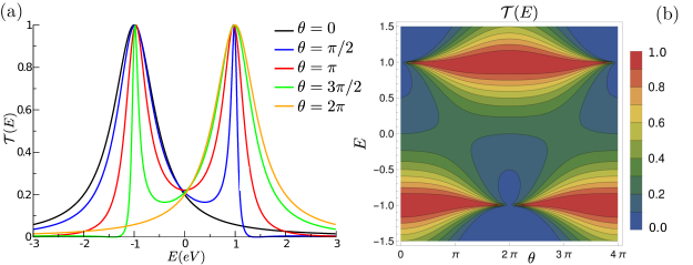
Figure 2: (a) Energy behavior of ${\mathcal{T}}(E)$ versus $E$ for different magnetic fluxes $\theta=2\pi\Phi(B)/\Phi_{0}$; (b) contour plot of ${\mathcal{T}}(E)$ as function of $\theta$ and $E$. The chosen parameters for the electronic system are $E_{d}=0$ eV, $t_{d}=-1$ eV and $\gamma=0.25$ eV.

III Structure of the transmission function and analytic evaluation of the kinetic parameters

Once the transmission function is known, we can access the kinetic transport coefficients that control, in the linear approximation, the thermoelectric properties of the nanoscale device. The kinetic transport coefficients, in dimensionless form, are linked to the transmission function ${\mathcal{T}}(E)$ by the relations:

$$K_{n}=\int_{-\infty}^{+\infty}dE\,{\mathcal{T}}(E)\,\frac{(E-\mu)^{n}}{(k_{B}T)^{n}}\,(-\frac{\partial f}{\partial E})\qquad(n=0,1,2)\ .$$ (31)

where $\mu$ is the chemical potential, $T$ the absolute temperature, and $f(E,\mu,T)$ the Fermi function.

In the literature, the evaluation of the kinetic coefficients $K_{0,1,2}$ is in general carried out either with the Sommerfeld expansion,ASHC possibly extended up to fourth order,SILVA12 or by numerical integration. A nice aspect of the Sommerfeld expansion is that the procedure is analytic; however it holds only at sufficiently low temperatures and reasonably smooth transmission function in the energy interval $k_{B}T$. The alternative procedure, based on numerical integration, requires particular caution because of the presence of sharp resonances and anti-resonance produced by the interference effects of the magnetic fields. This is an obstacle to the construction of counter plots or three dimensional graphics, often very useful to better illustrate at glance thermoelectric properties. The purpose of this section is to develop a brand new analytic procedure for the evaluation of the kinetic parameters, valid for any temperature range and applicable in any desired domain of the other parameters at play.

From the structure of Eq.(25) it is natural to define the kinetic functional of order $n$ as follows

$${\mathcal{F}}_{n}[\ldots]=\int_{-\infty}^{+\infty}dE\,[\ldots]\,\frac{(E-\mu)^{n}}{(k_{B}T)^{n}}\,(-\frac{\partial f}{\partial E})\quad,\quad f(E)=\frac{1}{e^{(E-\mu)/k_{B}T}+1}\ ,$$ (32)

where $[\ldots]$ stands for any arbitrary function of $E$ for which the integral exists. Then, the expression of the kinetic parameters of the symmetric double dot reads

$$K_{n}={\mathcal{F}}_{n}[{\mathcal{T}}(E)]\ ,$$ (33)

where ${\mathcal{T}}(E)$ is the transmission function reported in Eq.(18).

The first step to elaborate analytically the kinetic functionals requires the examination of the pole structure of ${\mathcal{T}}(E)$. The transmission function can in fact be resolved into the sum of just two simple poles, with appropriate weighting factors. This is shown in detail in Appendix A. According to Eq.(A10), the transmission function of the symmetric double dot can be cast in the form

$${\mathcal{T}}(E)=8\gamma^{2}\,{\rm Re}\left\{\frac{1}{A_{1}}\,\frac{[\cos(\theta/2)\,(E\!-\!E_{d})+t_{d}]^{2}}{E-z_{1}}+\frac{1}{A_{2}}\,\frac{[\cos(\theta/2)\,(E\!-\!E_{d})+t_{d}]^{2}}{E-z_{2}}\right\}$$ (34)

where the pole positions $z_{1,2}$ and the weighting factors $A_{12}$ are given by Eq.(A9).

Transmission function ${\mathcal{T}}(E)$ for the coupled degenerate double dot

${\mathcal{T}}(E)=8\gamma^{2}\,{\rm Re}\left\{\dfrac{1}{A_{1}}\,\dfrac{[\cos(\theta/2)\,(E\!-\!E_{d})+t_{d}]^{2}}{E-z_{1}}+\dfrac{1}{A_{2}}\,\dfrac{[\cos(\theta/2)\,(E\!-\!E_{d})+t_{d}]^{2}}{E-z_{2}}\right\}$

where $\quad\left\{\begin{array}[]{l}A_{1}=-16\,i\gamma\cos^{2}(\theta/4)\,[-i\gamma\cos(\theta/2)+t_{d}]\,[-i\gamma+t_{d}]\\[5.69054pt] A_{2}=-16\,i\gamma\sin^{2}(\theta/4)\,[+i\gamma\cos(\theta/2)-t_{d}]\,[-i\gamma-t_{d}]\\[5.69054pt] z_{1}=E_{d}+t_{d}-i\gamma-i\gamma\cos(\theta/2)\\[5.69054pt] z_{2}=E_{d}-t_{d}-i\gamma+i\gamma\cos(\theta/2)\ .\end{array}\right.$

Dimensionless kinetic parameters for the degenerate double dot system in the linear regime: $K_{n}=\int dE\,{\mathcal{T}}(E)\dfrac{(E-\mu)^{n}}{(k_{B}T)^{n}}(-\dfrac{\partial f}{\partial E})$ $\begin{array}[]{l}\vspace{1mm}K_{0}=8\gamma^{2}\,{\rm Re}\,\biggl{\{}\dfrac{1}{A_{1}}\biggl{[}\cos^{2}(\theta/2)\,(\mu+z_{1}-2E_{d})+2\cos(\theta/2)\,t_{d}\biggr{.}\biggr{.}\\ \hskip 85.35826pt+\biggl{.}\biggl{.}\dfrac{\left[\cos(\theta/2)\,(z_{1}-E_{d})+t_{d}\right]^{2}}{k_{B}T}\,I_{0}(\dfrac{z_{1}-\mu}{k_{B}T})\biggr{]}+\dfrac{1}{A_{2}}[the\ same\ with\ z_{2}]\biggr{\}}\\[2.84526pt] K_{1}=8\gamma^{2}\,{\rm Re}\,\biggl{\{}\dfrac{1}{A_{1}}\biggl{[}\dfrac{\pi^{2}}{3}\cos^{2}(\theta/2)\,k_{B}T\biggr{.}\biggr{.}\\ \hskip 85.35826pt+\biggl{.}\biggl{.}\dfrac{\left[\cos(\theta/2)\,(z_{1}-E_{d})+t_{d}\right]^{2}}{k_{B}T}\,I_{1}(\dfrac{z_{1}-\mu}{k_{B}T})\biggr{]}+\dfrac{1}{A_{2}}[the\ same\ with\ z_{2}]\biggr{\}}\\[2.84526pt] K_{2}=8\gamma^{2}\,{\rm Re}\,\biggl{\{}\dfrac{1}{A_{1}}\biggl{[}\dfrac{\pi^{2}}{3}\cos^{2}(\theta/2)\,(\mu+z_{1}-2E_{d})+\dfrac{2\pi^{2}}{3}\cos(\theta/2)\,t_{d}\biggr{.}\biggr{.}\\ \hskip 85.35826pt+\biggl{.}\biggl{.}\dfrac{\left[\cos(\theta/2)\,(z_{1}-E_{d})+t_{d}\right]^{2}}{k_{B}T}\,I_{2}(\dfrac{z_{1}-\mu}{k_{B}T})\biggr{]}+\dfrac{1}{A_{2}}[the\ same\ with\ z_{2}]\biggr{\}}\end{array}$ $I_{0}(w)=\pm\dfrac{1}{2\pi i}\Psi_{t}\,(\dfrac{1}{2}\pm\dfrac{iw}{2\pi})\ \ \,\,\,{\rm Im}\,w\lessgtr 0;\ \ I_{1}(w)=1+wI_{0}(w);\ \ I_{2}(w)=w+w^{2}I_{0}(w)$

Table 1: Transmission function ${\mathcal{T}}(E)$ and kinetic integrals $K_{0,1,2}$ in analytic form of the symmetric double quantum dot, with two orbitals of the same diagonal energy $E_{d}$, coupled together by the off-diagonal hopping element $t_{d}$, in the wide band approximation of parameter $\gamma$. The phase $\theta$ equals $2\pi\Phi(B)/\Phi_{0}$, where $\Phi(B)$ is the flux of magnetic field through the nanodevice in units of a single quantum flux $\Phi_{0}$. The trigamma function is denoted with $\Psi_{t}$.

Equation (28) is fully equivalent to Eq.(18), but it enjoys the invaluable advantage to put in evidence its two pole analytic structure. This permits the straight evaluation of the kinetic parameters:

$$K_{n}={\mathcal{F}}_{n}[{\mathcal{T}}(E)] = 8\gamma^{2}\,{\rm Re}\,\left\{\frac{1}{A_{1}}{\mathcal{F}}_{n}\,\left[\frac{[\cos(\theta/2)\cdot(E-E_{d})+t_{d}]^{2}}{E-z_{1}}\right]\right.$$ (35)

$$\left.\hskip 56.9055pt+\frac{1}{A_{2}}{\mathcal{F}}_{n}\,\left[\frac{[\cos(\theta/2)\cdot(E-E_{d})+t_{d}]^{2}}{E-z_{2}}\right]\right\}.$$

The analytic expressions of the kinetic functionals entering Eq.(29) are provided in Appendix B. The results for $K_{0},K_{1},K_{2}$ are given by Eqs.(B11,B12,B13) respectively. The transmission function and the corresponding kinetic integrals of the symmetric double dot are summarized in Table I, for immediate reference. The procedure here outlined is of value not only for the present problem, but also because it provides useful guidelines for a number of more complex situations.

Expressions of the thermoelectric functions in terms of the kinetic parameters
$\sigma=K_{0}\,\dfrac{e^{2}}{h}$	$S=-\dfrac{K_{1}}{K_{0}}\,\dfrac{k_{B}}{e}$	$\kappa_{e}=T(K_{2}-\dfrac{K_{1}^{2}}{K_{0}})(\dfrac{k_{B}^{2}}{h})$
$\dfrac{{\mathcal{P}}}{\eta_{c}^{2}}=\dfrac{1}{4}\,T^{2}\,\dfrac{K_{1}^{2}}{K_{0}}\,\dfrac{k_{B}^{2}}{h}$	$L=\dfrac{\ K_{0}K_{2}-K_{1}^{2}\ }{K_{0}^{2}}\ \dfrac{k_{B}^{2}}{e^{2}}$	$p=\dfrac{K_{1}^{2}}{K_{0}K_{2}}\quad(0\leq p\leq 1)$
$ZT=\dfrac{K_{1}^{2}}{K_{0}K_{2}-K_{1}^{2}}=\dfrac{p}{1-p}$                                     $\dfrac{\eta}{\eta_{c}}=\dfrac{\sqrt{1+ZT}-1}{\sqrt{1+ZT}+1}=\dfrac{1-\sqrt{1-p}}{1+\sqrt{1-p}}$
Expressions of the thermoelectric natural units for nanoscale devices
$\dfrac{e^{2}}{h}=3.874046\cdot 10^{-5}\ \dfrac{\rm A}{\rm V}$ ;	$\dfrac{k_{B}}{e}=86.17\ \dfrac{\mu{\rm V}}{\rm K}$  ;	$\dfrac{k_{B}^{2}}{e^{2}}=74.25\cdot 10^{-10}\,\dfrac{{\rm V}^{2}}{{\rm K}^{2}}$ ;
$\dfrac{k_{B}^{2}}{h}=1.8\cdot 10^{6}\,\dfrac{\rm eV}{\rm sec}\cdot\dfrac{1}{\rm K^{2}}=0.288\,\dfrac{\rm pW}{\rm K^{2}}$ $\quad\Longrightarrow\dfrac{k_{B}^{2}T_{0}^{2}}{h}=1.8\cdot 10^{6}\,\dfrac{\rm eV}{\rm sec}=0.288\,{\rm pW}\quad(T_{0}=1K)$

Table 2: Transport parameters in the linear approximation for thermoelectric materials, with electronic transmission function ${\mathcal{T}}(E)$. The kinetic parameters $K_{0,1,2}$ are defined in dimensionless form. The electric conductance $\sigma$, Seebeck coefficient $S$, power-output ${\mathcal{P}}$, electronic thermal conductance $\kappa_{e}$, Lorenz number $L$, performance parameter $p$, figure of merit $ZT$ and efficiency ${\eta}$ are reported. The quantity $\eta_{c}$ denotes the Carnot efficiency $\eta_{c}=\Delta T/T$, where $\Delta T$ is the temperature difference between the hot reservoir and the cold one.

After achieving the task of a straight analytic evaluation of the kinetic parameters of the double quantum dot system as summarized in Table I, it becomes now routine to investigate the transport properties. Following closely Ref. NOI, , in Table II we report for sake of completeness the expressions of the electric and thermal conductances, of the Seebeck coefficient and the other transport parameters of interest, in terms of the kinetic coefficients $K_{0},K_{1,}$, and $K_{2}$.

In the next section we evaluate magneto transport properties of specific double dot devices, and discuss the variety and wealth of effects occurring in spite of the reasonable simplicity of the model.

IV Results and discussion

We begin to examine a realistic space domain for the thermoelectric device under attention. For molecular junctions, we can set $\gamma\approx 0.25\ {\rm eV}$ and $t_{d}\approx-1.0\ {\rm eV}$. The fact that $|t_{d}|>>\gamma$ (almost an order of magnitude) assures that in the transmission function the Lorentz lineshape and the Fano lineshape are in general well resolved, with linewidths $2\gamma\cos^{2}(\theta/4)$ and $2\gamma\sin^{2}(\theta/4)$, respectively, as it is seen from Eq.(20). The values of $\theta$ explored to better highlight periodicity as function of $\theta$, are in the whole range $[0,4\pi]$, and in particular $\theta=0,\pi/2,\pi,3\pi/2$ and $2\pi$. The range of $\theta$ from one flux to two flux quanta ($2\pi<\theta\leq 4\pi$) retraces back the range from one flux to zero, and does not need to be considered explicitly. The room temperature considered entails $k_{B}T=0.025\ {\rm eV}$. The dot energy $E_{d}$ is taken as the reference energy and set equal to zero. In summary,: the figures reported below in this section refer to the set of parameters $E_{d}=0$, $\gamma=0.25$ eV, $t_{d}=-1.0$ eV, $k_{B}T=0.025\ {\rm eV}$ and $\theta=0,\pi/2,\pi,3\pi/2$ and $2\pi$. When useful, other temperatures, phases or parameter domain have been explored and commented (but in general not explicitly reported).

In Fig.3 the thermoelectric functions of the c-2QD, for varying chemical potential $\mu$ and magnetic flux parameter $\theta$ are provided. The left panels show the landscape of electrical conductivity $\sigma$, electrical thermal conductivity $\kappa_{e}$, Seebeck coefficient $S$, and figure of merit $ZT$. The right panels show sections of the same quantities for -2 eV$<\mu<$2 eV at $\theta=0,\pi/2,\pi,3\pi/2$ and $2\pi$, to better highlight their shape and symmetry. The curves profiles reported in the left panels respect the color sequence shown in the corresponding right panels. From Fig 3a and Fig.3b we observe that $\sigma$ and $\kappa_{e}$ have behavior similar to ${\mathcal{T}}$(E), as expected from their expressions; we also verified that the value of $\sigma$ increases (not shown in the figures) decreasing the temperature, and that the opposite occurs for $\kappa_{e}$.

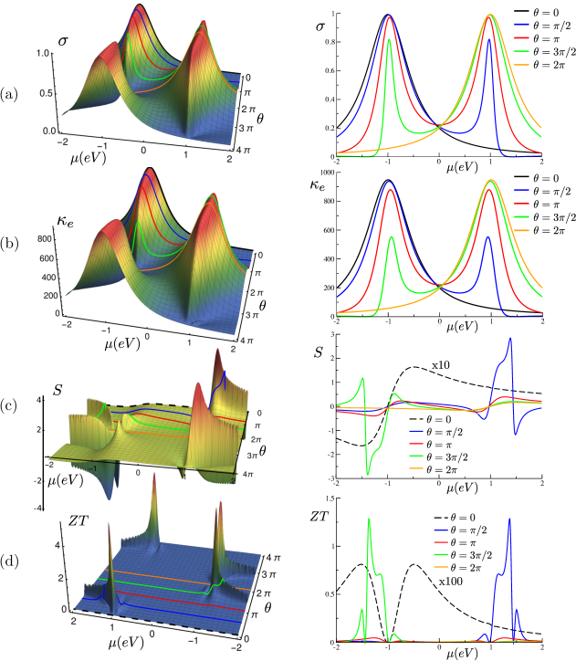
Figure 3: (a) Electrical conductivity $\sigma$ (in units ${e^{2}}/{h}$). (b) Electrical thermal conductivity $\kappa_{e}$ (in units ${k_{B}^{2}}T_{0}^{2}/{h}$). (c) Seebeck coefficient $S$ (in units ${k_{B}}/{e}$). (d) Figure of merit $ZT$ of the c-2QD under attention in the ($\mu-\theta$) plane. The left panels report the landscape of the thermoelectric functions in the ($\mu-\theta$) plane, the right panels report sections of the same quantities at $\theta=0,\pi/2,\pi,3\pi/2$ and $2\pi$. The black dashed lines in the right (c) and (d) panels evidence the results in the absence of magnetic flux. For $\theta=2\pi$ no multiplication by 10 or by 100 has been performed, to better emphasize the enhancement effect of the magnetic field. The colored curves in the left panels respect the sequence of the graphs shown in the corresponding right panels.

We observe that in the absence of magnetic field, i.e. $\theta$=0, ${\mathcal{T}}$(E) presents a Breit-Wigner resonance around $E_{b}=-1$ eV, and similarly $\sigma(\mu,0)$, and $\kappa_{e}(\mu,0)$ present a Breit-Wigner resonance around $\mu=E_{b}$. Moreover, near the resonant energy the thermopower $S$ vanishes while for $\mu\lesssim E_{b}$ ($\mu\gtrsim E_{b}$) $S$ is negative (positive), indicating mainly $n$-type ($p$-type) behavior of the device. The figure of merit $ZT$ vanishes where $S$ vanishes as expected from its definition, and remains small ($<0.01$) for any $\mu$. As temperature increases both $S$ and $ZT$ values increase.

When the magnetic field is switched on, both Breit-Wigner- and Fano-like resonances may contribute to the transmission spectra. In particular, for $\theta=2n\pi$, with $n$ integer number, only Breit-Wigner resonances occur, which are located at the bonding energy for $n$ even and at the antibonding energy for $n$ odd [see Eq. (21) and Eq. (22)]. For $\theta=(\pi/2+n\pi)$ both Breit-Wigner- and Fano-like resonances are present in the ${\mathcal{T}}$(E) spectrum, with Breit-Wigner (Fano) features centered at the bonding (antibonding) energies for $n$ even and viceversa for $n$ odd. We notice that ${\mathcal{T}}$(E) is symmetric around $E_{d}$ for $\theta=\pi$ or $\theta=(2n+1)\pi$ as required by Eq. (23). It is important to observe that $|S|$ increases by more than 10 times and $ZT$ by more than 100 times with respect to the case $\theta=0$, for specific values of the magnetic flux threading the c-2QD circuit as evidenced in the plots in the right side of Fig.3c and Fig.3d. In particular $|S|$ assumes large values ($\approx 4$ k_B/e) in the regions around $\theta\sim\pi/2$ and $\theta\sim 3\pi/2$ in the resonance and in the antiresonance regions. The above results are in agreement with the ones obtained for the benzene molecule junction in magnetic flux.LI17 Fig.3d shows that for the chosen $T$ and $\gamma$ parameters, $ZT$ can reach values $\approx 6$ in the regions $\theta\sim\pi/2$ and $\theta\sim 3\pi/2$. The above results evidence that temperature and magnetic flux can be exploited to increase the thermoelectric factor of merit .

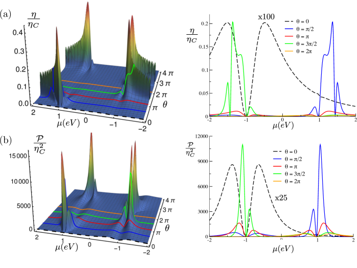
Figure 4: (a) Thermoelectric efficiency $\eta/\eta_{c}$ in the ($\mu-\theta$) plane. b) Output power ${\mathcal{P}}/\eta_{c}^{2}$ (in units $k_{B}^{2}T_{0}^{2}/h$). The left panels of Fig.4a and Fig.4b report the landscape of the thermoelectric efficiency and power output in the ($\mu-\theta$) plane, the right panels report sections of the same quantities at $\theta=0,\pi/2,\pi,3\pi/2$ and $2\pi$. The black dashed lines in the right panels evidence the results in the absence of magnetic flux.

Most interesting is the evaluation of the performance of the c-2QD as heat engine, in this case a study of the efficiency at the maximum output power is required. Several recent papers LINKE05 ; NAP10 ; ESP10 ; WIT13 ; HER13 ; LUO16 have shown that the mere knowledge of the maximum efficiency of a heat engine is of limited importance since the useful operative information concerns the conditions corresponding to the maximum power output.CA75 ; CASATI17 It is known in fact,that even if the figure of merit $ZT$ of a thermoelectric device can assume large values ($>>$1) mainly for nanostructured systemsWIERB11 ; VAR01 ; MUR08 , what really matters is just the efficiency evaluated at the maximum power output. To better clarify this point, we report in Fig.4a the thermoelectric efficiency and in Fig.4b the output power, respectively, as function of $\mu$ and $\theta$, as defined in Table II.

Once again we observe that the magnetic field strongly enhances the thermoelectric efficiency by more than two orders of magnitude with respect to the case of absence of magnetic field, in the resonance and antiresonance regions, while output power increases more than 25 times and can assume values of the order of $10^{4}$ (in units $k_{B}^{2}T_{0}^{2}/h$). Fig.5 summarizes the results of the evaluation of the efficiency at the maximum power output, which is the most appropriate metric to measure the performance of the device. For this aim we have scanned the flux $\theta$ parameter in the [0-4$\pi$] range and, for any $\theta$, we have looked for the maximum output power for varying values of the chemical potential $\mu$. This has allowed to evaluate the efficiency for the values of $\theta$ and $\mu$ which determine the maximum power conditions.

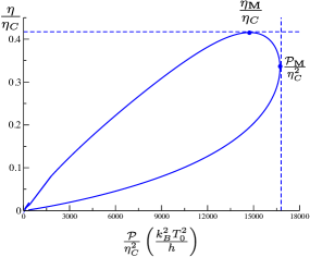
Figure 5: Maximum efficiency at the maximum output power. ${\mathcal{P}}_{M}/\eta_{C}^{2}$ is the highest value of the output power; $\eta_{M}/\eta_{C}$ is the maximum value of the device efficiency.

The set of all the maximum power and corresponding efficiency data have been exploited to produce Fig.5 which reports the curve of the maximum efficiency at the maximum output power. From Fig.5 we can observe that the maximum efficiency is higher than the efficiency at operating conditions where the maximum output power is realized We can see that the highest value of the power output ${\mathcal{P}}_{M}/\eta_{C}^{2}$ is 16800 (in units $k_{B}^{2}T_{0}^{2}/h$) for the values $\theta\approx 1$, and $\theta\approx(4\pi-1)$, at $\mu\approx 1.062$ eV, and for $\theta\approx(2\pi-1)$ and $\theta\approx(2\pi+1)$, at $\mu\approx-1.062$ eV. Correspondingly, the normalized efficiency at maximum power is $\eta({\mathcal{P}}_{M})/\eta_{C}$=0.33. Moreover, we can see that the highest value of efficiency $\eta_{M}/\eta_{C}$ is 0.43 which occurs for the values $\theta\approx\pi/4$ and $15\pi/4$, at $\mu\approx 1.068$ eV and for $\theta\approx 7\pi/4$ and $9\pi/4$, at $\mu\approx-1.068$ eV. Correspondingly, the power output is ${\mathcal{P}}(\eta_{M})/\eta_{C}^{2}=14200$ (in units $k_{B}^{2}T_{0}^{2}/h$).

V Conclusions

We have presented in this paper a systematic analytic study of the thermoelectric response functions of a coupled double quantum dot system, pierced by a magnetic field, connected to left and right reservoirs, in the linear regime. Our method is based on the Green^′s function formalism. The results are analytic and can be expressed in terms of easily accessible trigamma functions and Bernoulli numbers; this has allowed to scan wide ranges of values of chemical potentials and temperatures of the reservoirs, different threading magnetic fluxes, dot energies and interdot interactions. Our results show that thermoelectric transport through the c-2QD can be strongly enhanced by the magnetic flux, mainly in the energy regions around the bonding and antibonding resonances of the system, which can be experimentally reached varying the system chemical potential by appropriate gate. The thermopower $S$ can be enhanced by more than ten times and the figure of merit $ZT$ by more than hundred times by the presence of a threading magnetic field. Most important, we have also found in this simple system that the magnetic flux increases the performance of the device under maximum power output conditions.

Appendix A. Transforming product of simple poles into the weighted sum of simple poles

The purpose of this Appendix is to transform a product of simple poles into the fully equivalent (and much more convenient) weighted sum of simple poles. Without entering into technicalities and subtleties, we confine our attention to the case of four poles, just of actual interest for double dots. We start from the identity

$$\frac{1}{(E\!-\!z_{1})(E\!-\!z_{2})(E\!-\!z_{3})(E\!-\!z_{4})}\equiv\frac{1}{A_{1}}\frac{1}{E\!-\!z_{1}}\!+\!\frac{1}{A_{2}}\frac{1}{E\!-\!z_{2}}\!+\!\frac{1}{A_{3}}\frac{1}{E\!-\!z_{3}}\!+\!\frac{1}{A_{4}}\frac{1}{E\!-\!z_{4}}$$ (A1)

where the $A_{1,2,3,4}$ constants (i.e. independent from the energy variable) have the expressions

$$\left\{\begin{array}[]{lll}A_{1}&=&(z_{1}-z_{2})(z_{1}-z_{3})(z_{1}-z_{4})\\[2.84526pt] A_{2}&=&(z_{2}-z_{1})(z_{2}-z_{3})(z_{2}-z_{4})\\[2.84526pt] A_{3}&=&(z_{3}-z_{1})(z_{3}-z_{2})(z_{3}-z_{4})\\[2.84526pt] A_{4}&=&(z_{4}-z_{1})(z_{4}-z_{2})(z_{4}-z_{3})\end{array}\right.\ .$$ (A6)

It is seen that the $A_{i}$ constant is the product of the differences of $z_{i}$ with all the other poles $z_{j}(\neq z_{i})$, except $z_{i}$ itself.

To demonstrate the identity (A1), suppose to multiply both members of Eq.(A1) by the expression $\Pi_{i=1,4}(E-z_{i})$. After multiplication, the first member becomes independent from $E$, and equal to unit. This occurs also for the second member. In fact after multiplication, the second member becomes a polynomial in $E$ of order three, which takes the unity value at the four arguments $E=z_{1},z_{2},z_{3},z_{4}$, and is thus unity everywhere.

Case of complex conjugate poles

In the case of complex conjugate poles, say $(z_{1},z_{2},z_{3}=z_{1}^{\ast},\ z_{4}=z_{2}^{\ast})$, it is seen by inspection that Eqs.(A1,A2) simplify in the form

$$\frac{1}{(E-z_{1})(E-z_{2})(E-z_{1}^{\ast})(E-z_{2}^{\ast})}\equiv 2\,{\rm Re}\,\left[\frac{1}{A_{1}}\frac{1}{E-z_{1}}+\frac{1}{A_{2}}\frac{1}{E-z_{2}}\right],$$ (A7)

where the $A_{1,2}$ constants have the expressions

$$\left\{\begin{array}[]{lll}A_{1}&=&(z_{1}-z_{2})(z_{1}-z_{1}^{\ast})(z_{1}-z_{2}^{\ast})\\[2.84526pt] A_{2}&=&(z_{2}-z_{1})(z_{2}-z_{1}^{\ast})(z_{2}-z_{2}^{\ast})\end{array}\right..$$ (A10)

Pole structure of the double dot transmission function

The expression of the transmission function of the symmetric double dot is provided in Eq.(18), and can be written in the form

$${\mathcal{T}}(E)=\frac{4\gamma^{2}}{D^{R}(E)D^{A}(E)}\left[\cos(\theta/2)\cdot(E-E_{d})+t_{d}\right]^{2}$$ (A11)

where $D^{A}(E)=[D^{R}(E)]^{*}$, and

$$D^{R}(E)=[E-E_{d}-t_{d}+i\gamma+i\gamma\cos(\theta/2)]\,[E-E_{d}+t_{d}+i\gamma-i\gamma\cos(\theta/2)]\ .$$ (A12)

The analytic structure of the transmission function can be put in better evidence by expressing $D^{R}(E)$ in the form

$$D^{R}(E)=(E-z_{1})(E-z_{2})\qquad\left\{\begin{array}[]{l}z_{1}=E_{d}+t_{d}-i\gamma-i\gamma\cos(\theta/2)\\[5.69054pt] z_{2}=E_{d}-t_{d}-i\gamma+i\gamma\cos(\theta/2)\end{array}\right.\ ,$$ (A13)

and similarly for its complex conjugate $D^{A}(E)$. Using Eqs.(A3,A4,A7) one obtains

$$\frac{1}{D^{R}(E)D^{A}(E)}\equiv 2\,{\rm Re}\,\left[\frac{1}{A_{1}}\frac{1}{E-z_{1}}+\frac{1}{A_{2}}\frac{1}{E-z_{2}}\right]\ ,$$ (A14)

where

$$\left\{\begin{array}[]{rcl}A_{1}&=&-16\,i\gamma\cos^{2}(\theta/4)\,[\,\,t_{d}-i\gamma\cos(\theta/2)\,\,]\,[\,\,t_{d}-i\gamma\,\,]\\[5.69054pt] A_{2}&=&-16\,i\gamma\sin^{2}(\theta/4)\,[-t_{d}+i\gamma\cos(\theta/2)]\,[-t_{d}-i\gamma]\\[5.69054pt] z_{1}&=&E_{d}+t_{d}-i\gamma-i\gamma\cos(\theta/2)\\[5.69054pt] z_{2}&=&E_{d}-t_{d}-i\gamma+i\gamma\cos(\theta/2)\ .\end{array}\right.$$ (A15)

The transmission function of the symmetric double can be expressed in the form

$${\mathcal{T}}(E)\!=\!8\gamma^{2}\,{\rm Re}\left\{\frac{1}{A_{1}}\,\frac{[\cos(\theta/2)\,(E\!-\!E_{d})+t_{d}]^{2}}{E-z_{1}}+\frac{1}{A_{2}}\,\frac{[\cos(\theta/2)\,(E\!-\!E_{d})+t_{d}]^{2}}{E-z_{2}}\right\}$$ (A16)

Eq.(A10) shows explicitly the pole structure of the transmission function, and is ready for analytic evaluation of the corresponding kinetic integrals.

Appendix B. Kinetic functional for the analytic treatment of thermoelectricity in double dots

For the analytic treatment of thermoelectricity in double dots, it is convenient to define the kinetic functional as follows

$${\mathcal{F}}_{n}[\ldots]=\int_{-\infty}^{+\infty}dE\,[\ldots]\,\frac{(E-\mu)^{n}}{(k_{B}T)^{n}}\,(-\frac{\partial f}{\partial E})\qquad f(E)=\frac{1}{e^{(E-\mu)/k_{B}T}+1}\ ,$$ (B1)

where $[\ldots]$ stands for any arbitrary function of $E$, for which the integral in Eq.(B1) exists, and $n=0,1,2,...$. What is needed are just the kinetic functionals of polynomials in energy, and their product by a simple pole. The results are of interest not only in the model nanostructure under attention, but also in other more general and complex models.

Kinetic functional of a constant and of the variable itself

Due to the fact that the functional (B1) is linear, the functional of a constant equals the functional of unity times the constant. The functional of unity is

$${\mathcal{F}}_{n}\left[1\right] = \int_{-\infty}^{+\infty}dE\,\frac{(E-\mu)^{n}}{(k_{B}T)^{n}}\,(-\frac{\partial f}{\partial E})\qquad f(E)=\frac{1}{e^{(E-\mu)/k_{B}T}+1}$$ (B2)

$$= \int_{-\infty}^{+\infty}dE\,\frac{(E-\mu)^{n}}{(k_{B}T)^{n}}\,\frac{1}{k_{B}T}\frac{e^{(E-\mu)/k_{B}T}}{[e^{(E-\mu)/k_{B}T}+1]^{2}}\quad;\quad set\quad z=\frac{E-\mu}{k_{B}T}\ ;$$

$$= \int_{-\infty}^{+\infty}dz\,z^{n}\,\frac{e^{z}}{(e^{z}+1)^{2}}\equiv b_{n}\ .$$

Thus the kinetic functionals of unity equal the Bernoulli-like numbers. The first few Bernoulli-like numbers $b_{n}$ are

$$b_{0}=1\ ,\ b_{1}=0\ ,\ b_{2}=\frac{\pi^{2}}{3}\ ,\ b_{3}=0\ ,\ b_{4}=\frac{7\pi^{4}}{15}\ ,\ b_{5}=0\ ,\ b_{6}=\frac{31\pi^{6}}{21}\ \ldots\$$ (B3)

[For details see Ref.GRAD, ].

The kinetic functional of the energy is easily obtained, using again the linear properties of the functional. It holds

$${\mathcal{F}}_{n}\left[E-E_{d}\right]={\mathcal{F}}_{n}\left[(E-\mu)+\mu-E_{d}\right]=k_{B}T\,{\mathcal{F}}_{n}\left[\frac{E-\mu}{k_{B}T}\right]+(\mu-E_{d})\,{\mathcal{F}}_{n}[1]\ .$$

It follows

$${\mathcal{F}}_{n}\left[E-E_{d}\right]=k_{B}T\,b_{n+1}+(\mu-E_{d})\,b_{n}\ .$$ (B4)

Kinetic functional of a simple pole

Consider the simple pole function of the form

$$X_{0}(E)=\frac{1}{E-z_{p}}\ ,$$ (B5)

where $z_{p}$ is a given position in the upper or lower part of complex plane. The kinetic functional becomes

$${\mathcal{F}}_{n}\left[\frac{1}{E-z_{p}}\right]=\int_{-\infty}^{+\infty}dE\,\frac{1}{E-z_{p}}\,\frac{(E-\mu)^{n}}{(k_{B}T)^{n}}\,\frac{1}{k_{B}T}\frac{e^{(E-\mu)/k_{B}T}}{[e^{(E-\mu)/k_{B}T}+1]^{2}}\ .$$

As usual, it is convenient to introduce the dimensionless variables

$$z=\frac{E-\mu}{k_{B}T}\quad;\quad dz=\frac{dE}{k_{B}T}\quad;\quad E=k_{B}T\,z+\mu\ .$$

With the indicated substitutions, one obtains

$${\mathcal{F}}_{n}\left[\frac{1}{E-z_{p}}\right] = \int_{-\infty}^{+\infty}dz\,\frac{z^{n}}{\,k_{B}T\,z+\mu-z_{p}\,}\,\frac{e^{z}}{(e^{z}+1)^{2}}$$

$$= \frac{1}{k_{B}T}\int_{-\infty}^{+\infty}dz\,\frac{z^{n}}{z-(z_{p}-\mu)/k_{B}T}\,(-\frac{\partial f}{\partial z})\quad\ f(z)=\frac{1}{e^{z}+1}$$

$$= \frac{1}{k_{B}T}\int_{-\infty}^{+\infty}dz\,\frac{z^{n}}{z-w_{p}}\,(-\frac{\partial f}{\partial z})\qquad\quad w_{p}=\frac{z_{p}-\mu}{k_{B}T}\ .$$

In summary, it holds

$${\mathcal{F}}_{n}\left[\frac{1}{E-z_{p}}\right]\equiv\frac{1}{k_{B}T}\,J_{n}(w_{p})\qquad,\qquad w_{p}=\frac{z_{p}-\mu}{k_{B}T}\ ,$$ (B6)

where $J_{n}$ denote the complex functions

$$J_{n}(w)=\int_{-\infty}^{+\infty}dz\,\frac{z^{n}}{z-w}\,(-\frac{\partial f}{\partial z})\qquad n=0,1,2,\ldots$$

The first few $J$-functions are

$$J_{0}(w)=\pm\frac{1}{2\pi i}\Psi_{t}\,(\frac{1}{2}\pm\frac{iw}{2\pi})\ \ {\rm Im}\,w\lessgtr 0\ \ ;\ \ J_{1}(w)=1+wJ_{0}(w)\ \ ;\ \ J_{2}(w)=w+w^{2}J_{0}(w)\ ,$$

where

$$\Psi_{t}(z)=\sum_{n=0}^{\infty}\,\frac{1}{(z+n)^{2}}$$

is the trigamma function. The trigamma function is a one-valued analytic function with poles of order two at the points $z=0,-1,-2,...$, and routinely available in computer libraries. For details on the digamma, trigamma and poligamma functions see Ref.ABRA,

Trigamma function and Bernoulli-like numbers are the ingredients for the analytic evaluation of the kinetic functional of interest, including the next ones.

Kinetic functional of a simple pole times the first and second power of the energy

Consider the function of the form

$$X_{1}(E)=\frac{E-E_{d}}{E-z_{p}}\ ,$$

where $z_{p}$ is the position of the pole in the upper or lower part of complex plane, and $E_{d}$ is an arbitrary complex constant. We have

$${\mathcal{F}}_{n}\left[\frac{E-E_{d}}{E-z_{p}}\right]={\mathcal{F}}_{n}\left[\frac{(E-z_{p})+z_{p}-E_{d}}{E-z_{p}}\right]={\mathcal{F}}_{n}\left[1\right]+(z_{p}-E_{d})\,{\mathcal{F}}_{n}\left[\frac{1}{E-z_{p}}\right].$$

It follows

$${\mathcal{F}}_{n}\left[\frac{E-E_{d}}{E-z_{p}}\right]=b_{n}+\frac{z_{p}-E_{d}}{k_{B}T}\,I_{n}(w_{p})\qquad;\qquad w_{p}=\frac{z_{p}-\mu}{k_{B}T}\ .$$ (B7)

Another function to consider is

$$X_{2}(E)=\frac{(E-E_{d})^{2}}{E-z_{p}}\ ,$$

where $z_{p}$ is a given position in the upper or lower part of complex plane. The kinetic functional can be cast in the form

$${\mathcal{F}}_{n}\left[\frac{(E-E_{d})^{2}}{E-z_{p}}\right] = {\mathcal{F}}_{n}\left[E+z_{p}-2E_{d}+\frac{(z_{p}-E_{d})^{2}}{E-z_{p}}\right]$$

$$= {\mathcal{F}}_{n}\left[E-E_{d}\right]+(z_{p}-E_{d})\,{\mathcal{F}}_{n}\left[1\right]+(z_{p}-E_{d})^{2}\,{\mathcal{F}}_{n}\left[\frac{1}{E-z_{p}}\right].$$

Using previous results we obtain

$${\mathcal{F}}_{n}\left[\frac{(E-E_{d})^{2}}{E-z_{p}}\right]=k_{B}T\,b_{n+1}+(\mu+z_{p}-2E_{d})\,b_{n}+\frac{(z_{p}-E_{d})^{2}}{k_{B}T}\,I_{n}(w_{p})\ .$$ (B8)

We could proceed with higher powers along similar lines, whenever needed.

Analytic expression of the kinetic integrals for the symmetric double dot

According to Eq.(29), the kinetic integrals for the symmetric double are given by the expression

$$K_{n}\!=\!8\gamma^{2}\,{\rm Re}\left\{\frac{1}{A_{1}}{\mathcal{F}}_{n}\left[\frac{[\cos(\theta/2)\cdot(E\!-\!E_{d})+t_{d}]^{2}}{E-z_{1}}\right]+\frac{1}{A_{2}}{\mathcal{F}}_{n}[the\ same\ with\ z_{2}]\right\}$$ (B9)

The first functional in the above equation, using Eqs.(B6),(B7),(B8), reads

$${\mathcal{F}}_{n}\left[\frac{\left[\cos(\theta/2)\,(E-E_{d})+t_{d}\right]^{2}}{E-z_{1}}\right] = \cos^{2}(\theta/2)\left[k_{B}T\,b_{n+1}+(\mu+z_{1}-2E_{d})\,b_{n}\right]$$ (B10)

$$+2\cos(\theta/2)\,t_{d}b_{n}+\frac{[\cos(\theta/2)\,(z_{1}-E_{d})+t_{d}]^{2}}{k_{B}T}\,J_{n}(\frac{z_{1}-\mu}{k_{B}T})\ .$$

It is convenient to write more explicitly the first few values $F_{0,1,2}$. Using Eqs.(B3) we obtain the expressions:

$${\mathcal{F}}_{0}\left[\frac{\left[\cos(\theta/2)\,(E-E_{d})+t_{d}\right]^{2}}{E-z_{1}}\right] = \cos^{2}(\theta/2)\,(\mu+z_{1}-2E_{d})+2\cos(\theta/2)\,t_{d}$$

$$+\ \frac{\left[\cos(\theta/2)\,(z_{1}-E_{d})+t_{d}\right]^{2}}{k_{B}T}\,J_{0}(\frac{z_{1}-\mu}{k_{B}T})\ .$$

Similarly:

$${\mathcal{F}}_{1}\left[\frac{\left[\cos(\theta/2)\,(E-E_{d})+t_{d}\right]^{2}}{E-z_{1}}\right] = \frac{\pi^{2}}{3}\cos^{2}(\theta/2)\,k_{B}T$$

$$+\ \frac{\left[\cos(\theta/2)\,(z_{1}-E_{d})+t_{d}\right]^{2}}{k_{B}T}\,J_{1}(\frac{z_{1}-\mu}{k_{B}T})\ .$$

It also holds

$${\mathcal{F}}_{2}\left[\frac{\left[\cos(\theta/2)\,(E-E_{d})+t_{d}\right]^{2}}{E-z_{1}}\right] = \frac{\pi^{2}}{3}\cos^{2}(\theta/2)\left(\mu+z_{1}-2E_{d}\right)$$

$$+\frac{2\pi^{2}}{3}\cos(\theta/2)\,t_{d}+\frac{\left[\cos(\theta/2)\,(z_{1}-E_{d})+t_{d}\right]^{2}}{k_{B}T}\,J_{2}(\frac{z_{1}-\mu}{k_{B}T})\ .\quad$$

Inserting the above result into Eq.(B9) provides the analytic expression of the kinetic parameters. It holds:

$$K_{0} = 8\gamma^{2}\,{\rm Re}\,\left\{\frac{1}{A_{1}}\left[\cos^{2}(\theta/2)\,(\mu+z_{1}-2E_{d})+2\cos(\theta/2)\,t_{d}\right.\right.$$ (B11)

$$+ \left.\left.\frac{\left[\cos(\theta/2)\,(z_{1}-E_{d})+t_{d}\right]^{2}}{k_{B}T}\,J_{0}(\frac{z_{1}-\mu}{k_{B}T})\right]+\frac{1}{A_{2}}[the\ same\ with\ z_{2}]\right\}.\quad$$

The next kinetic parameter reads

$$K_{1} = 8\gamma^{2}\,{\rm Re}\,\left\{\frac{1}{A_{1}}\left[\frac{\pi^{2}}{3}\cos^{2}(\theta/2)\,k_{B}T\right.\right.$$ (B12)

$$+ \left.\left.\frac{\left[\cos(\theta/2)\,(z_{1}-E_{d})+t_{d}\right]^{2}}{k_{B}T}\,J_{1}(\frac{z_{1}-\mu}{k_{B}T})\right]+\frac{1}{A_{2}}[the\ same\ with\ z_{2}]\right\}.\quad$$

The third kinetic parameter of interest is

$$K_{2} = 8\gamma^{2}\,{\rm Re}\,\left\{\frac{1}{A_{1}}\left[\frac{\pi^{2}}{3}\cos^{2}(\theta/2)\,(\mu+z_{1}-2E_{d})+\frac{2\pi^{2}}{3}\cos(\theta/2)\,t_{d}\right.\right.$$ (B13)

$$+ \left.\left.\frac{\left[\cos(\theta/2)\,(z_{1}-E_{d})+t_{d}\right]^{2}}{k_{B}T}\,J_{2}(\frac{z_{1}-\mu}{k_{B}T})\right]+\frac{1}{A_{2}}[the\ same\ with\ z_{2}]\right\}.\quad$$

For convenience the basic results for actual simulations are summarized in Table I.

Acknowledgments The authors acknowledge the “IT center” of the University of Pisa for the computational support.

REFERENCES

REFERENCES

(1) L. D. Hicks and M. S. Dresselhaus, Phys. Rev. B 47, 12727 (1993).
(2) D. Sánchez and H. Linke, New J. Phys. 16, 110201 (2014).
(3)B. B. Brogi, S. Chand, and P. K. Ahluwalia, Physica B 461, 110 (2015).
(4)K. Kang and S. Y. Cho, J. Phys.: Condens. Matter 16, 117 (2004).
(5)B. Kubala and J. König, Phys. Rev. B 65, 245301 (2002).
(6)Ya. M. Blanter, C. Bruder, R. Fazio, and H. Schoeller, Phys. Rev. B 55, 4069 (1997).
(7) M. L. Ladrón de Guevara, F. Claro, and P. A. Orellana, Phys. Rev. B 67, 195335 (2003).
(8) G. Gómez-Silva, O. Ávalos-Ovando, M. L. Ladrón de Guevara, and P. A. Orellana, J. App. Phys. 111, 053704 (2012).
(9) M. Wierzbicki and R. Swirkowicz, Phys. Rev. B 84, 075410 (2011).
(10) V. M. García-Suárez, R. Ferradás, and J. Ferrer, Phys. Rev. B 88, 235417 (2013).
(11)Q. Wang, H. Xie, Y-H. Nie, and W. Ren, Phys. Rev. B 87, 075102 (2013).
(12) P. A. Orellana, M. L. Ladrón de Guevara, and F. Claro, Phys. Rev. B 70, 233315 (2004).
(13) P. P. Hofer and B. Sothmann, Phys. Rev. B 91, 195406 (2015)
(14) P. Samuelsson, S. Kheradsoud, and B. Sothmann, Phys. Rev. Lett. 118, 256801 (2017).
(15) Bogdan R. Bulka and Tomasz Kostyrko, Phys. Rev. B 70, 205333 (2004).
(16)M. A. Sierra, M. Saiz-Bretín, F. Domínguez-Adame, and D. Sánchez, Phys. Rev. B 93, 235452 (2016).
(17) Z.-M. Bai, M.-F. Yang, and Y.-C. Chen, J. Phys.: Condens. Matter 16, 2053 (2004).
(18) Y. S. Liu and X. F. Yang, J. App. Phys. 108, 023710 (2010).
(19) M. Pylak and R. Svirkowicz, Phys. Status Solidi B 247, 122 (2010).
(20) B. Sothmann, R. Sánchez and A. N. Jordan,
Nanotechnology 26, 032001 (2015).
(21)C. J. Lambert, H. Sadeghi, and Q.H. Al-Galiby, Comptes Rendus Physique 17, 1084 (2016).
(22)
J. Argüello-Luengo, D. Sánchez, and R. López, Phys. Rev. B 91, 165431 (2015).
(23) I. S. Gradshteyn and I. M. Ryzhik, Tables of Integrals,
Series and Products, Academic Press (New York, 1980).
(24) M. Abramowitz and I. A. Stegun, Handbook of Mathematical Functions (Dover, New York, 1972).
(25) P. Butcher, J. Phys. Cond. Matter 2, 4869 (1990).
(26) G. Bevilacqua, G. Grosso, G. Menichetti, and G. Pastori Parravicini, Phys. Rev. B 94, 245419 (2016).
(27) G. Grosso and G. Pastori Parravicini Solid State Physics, (Elsevier-Academic, Oxford 2014) second edition.
(28) D. K. Ferry, S. M. Goodnick, and J. Bird, Transport in Nanostructures, 2nd edn. (Cambridge University Press, New York, 2009).
(29)S. Datta, Electronic transport in Mesoscopic Systems, (Cambridge University Press, Cambridge,1997); Quantum Transport: Atom to Transistor, (Cambridge University Press, Cambridge, 2005).
(30) N. W. Ashcroft and N. D. Mermin, Solid State Physics, (Holt, Rinehart and Winston, New York, 1976).
(31) H. Li, Y. Wang, X. Kang, S. Liu, and R. Li, J. App. Phys. 121, 065105 (2017).
(32) T. E. Humphrey and H. Linke, Phys. Rev. Lett. 94, 096601 (2005).
(33) N. Nakpathomkun, H. Q. Xu, and H. Linke, Phys. Rev. B 82, 235428 (2010).
(34) M. Esposito, R. Kawai, K. Lindenberg, and C. Van den Broeck, Phys. Rev. Lett. 105, 150603 (2010).
(35) R. S. Whitney, Phys. Rev. Lett. 112, 130601 (2014).
(36) S. Hershfield, K. A. Muttalib, and B. J. Nartowt, Phys. Rev. B 88, 085426 (2013).
(37) X. Luo, N. Liu, and T. Qiu, Phys. Rev. E 93, 032125 (2016).
(38) F. L. Curzon and B. Ahlborn, Am. J. Phys. 43, 22 (1975).
(39) G. Benenti, G. Casati, K. Saito, and R. S. Whitney, Physics Reports 694, 1 (2017).
(40) R. Venkatasubramanian, E. Siivola, T. Colpitts, and B. O’Quinn, Nature 413, 597 (2001).
(41) P. Murphy, S. Mukerjee, and J Moore, Phys. Rev. B 78, 161406(R) (2008).