A new Bernstein-type operator based on Pólya’s urn model with negative replacement

Abstract.

Using Pólya’s urn model with negative replacement we introduce a new Bernstein-type operator and we show that the new operator improves upon the known estimates for the classical Bernstein operator. We also provide numerical evidence showing that the new operator gives a better approximation when compared to some other classical Bernstein-type operators.

1. Introduction

About a hundred years ago, in his beautiful and short paper ([1], 2 pages), Serge Bernstein gave a (probabilistic) proof of Weierstrass’s theorem on uniform approximation by polynomials, with a constructive method of approximation, known nowadays as Bernstein’s polynomials.

The probabilistic idea behind Bernstein’s construction can be seen as follows. If $X_{n}$ is random variable with a binomial distribution with parameters $n\in\mathbb{N}^{\ast}$ (number of trials) and $p\in\left[0,1\right]$ (probability of success), then $E\left(\frac{X_{n}}{n}\right)=p$. Choosing $p=x\in\left[0,1\right]$, we have $E\left(\frac{X_{n}}{n}\right)=x$, and since the variance $\sigma^{2}\left(\frac{X_{n}}{n}\right)=\frac{x\left(1-x\right)}{n}$ is small for $n$ sufficiently large, heuristically we have $\frac{X_{n}}{n}\approx x$, and if $f:[0,1]\rightarrow\mathbb{R}$ is continuous we also have $f\left(\frac{X_{n}}{n}\right)\approx f\left(x\right)$. Taking expectation leads to Bernstein’s polynomials

$$B_{n}\left(f;x\right)=\sum_{k=0}^{n}f\left(\frac{k}{n}\right)C_{n}^{k}x^{k}\left(1-x\right)^{n-k}=Ef\left(\frac{X_{n}}{n}\right)\approx f(x),$$ (1.1)

and Bernstein’s proof shows that this intuition is indeed correct: if $f$ is continuous on $\left[0,1\right]$, then $B_{n}$ converges uniformly to $f$ on $\left[0,1\right]$ for $n\rightarrow\infty$.

Aside from their importance in Analysis, Bernstein’s polynomials generated an important area of research in various fields of Mathematics and Computer Science, which continues to develop even today. The Bernstein polynomials were intensively studied in Operator Theory and Approximation Theory, where they were generalized by several authors, for example by F. Schurer (Bernstein-Schurer operator, [23]), D. D. Stancu (Bernstein-Stancu operator, [25]), A. Lupaş (Lupaş operator, [13], and q-Bernstein operator, [14]), G. M. Phillips ($q$-Bernstein operator, [21]), M. Mursaleen et. al. ($\left(p,q\right)$-Bernstein operator, [16]), and many others. See also [4] for a recent survey of Bernstein polynomials from the historical prospective, of the properties and algorithms of interest in Computer Science, and of their various applications.

In the present paper we are concerned with a generalization of Bernstein polynomials based on Polya’s urn distribution with (negative) replacement, which to our knowledge is new in the literature, the primary interest being the study of a new operator obtained for a particular choice of parameters involved. Our main results (Theorem 5.2, Theorem 5.4, and Theorem 5.6) indicate that the new operator $R_{n}$ improves the approximation provided by the classical Bernstein operator, and the numerical results (Section 6) also show that the new operator gives a better approximation than some of the well-known Bernstein-type operators.

The structure of the paper is as follows. In Section 2 we set up the notation and we review the basic properties of the Pólya urn model, which will be used in the sequel.

In Section 3 we introduce the operator $P_{n}^{a,b,c}$ depending on $a,b\in\mathbb{R}_{+}$ and $c\in\mathbb{R}$ satisfying an additional hypothesis. Although for $c\geq 0$ the operator $P_{n}^{x,1-x,c}$ coincides with the classical Bernstein-Stancu operator ([25]), our primary interest in the present paper is to consider negative values of $c$, for which the resulting operator $R_{n}$ seems to have better approximation properties than other Bernstein-type operators (see Remark 3.1, and the results in Section 5 and Section 6).

The main properties of the operator $R_{n}$ are given in Section 4, Theorem 4.1.

In Section 5 we give the error estimates for the operator $R_{n}$. Using a probabilistic lemma which may be of independent interest (Lemma 5.1), in Theorem 5.2 we give a short proof of an error estimate for $R_{n}$ using the modulus of continuity. The constant involved ($C=\frac{31}{27}\approx 1.14815...$) is smaller than the corresponding constant in the case of Bernstein polynomial $B_{n}$ obtained by Popoviciu ($C=\frac{3}{2}$) and Lorentz ($C=\frac{5}{4}$), but it is sligtly larger than the optimal constant $C_{opt}\approx 1.08988...$ obtained by Sikkema. In a subsequent paper ([17]), we will show that the actual value of the constant is in fact smaller than the optimal constant obtained by Sikkema in the case of the classical Bernstein operator. In Theorem 5.4 we give the error estimate in the case of a continuously differentiable function, and in Theorem 5.6 we give the asymptotic behaviour of the error estimate in the case of a twice continuously differentiable function.

The paper concludes (Section 6) with several numerical results which also indicate that the operator $R_{n}$ provides a better approximation than other classical Bernstein-type operators, even for small values of $n$ or discontinuous functions.

2. Preliminaries

Pólya’s urn model (also known as Pólya-Eggenberger urn model, see [3], [19]) generalizes the classical urn model, in which one observes balls extracted from an urn containing balls of two colors. Urn models have been considered by various authors, including Bernstein ([2]) - see for example Friedman’s model ([5], or [6] for an extension of it), or the recent paper [7] on generalized Pólya urn models, and the references cited therein.

For sake of completeness, we briefly describe the Pólya’s urn model which will be used in the sequel. The simplest urn model is the case when balls are extracted successively from an urn containing balls of two colors ($a$ white balls and $b$ black balls, $a,b\in\mathbb{N}$), the extracted ball being returned to the urn before the next extraction. In this case, the number of white balls in $n\geq 1$ extractions from the urn follows a binomial distribution with parameters $n$ and $p=\frac{a}{a+b}$ (considering the extraction of a white ball a “success”).

In Pólya’s urn model, the extracted ball is returned to the urn together with $c$ balls of the same color, the case of a negative integer $c\in\mathbb{Z}$ being interpreted as removing $\left|c\right|$ balls from the urn. When $c$ is negative, the model breaks down if there are insufficient many balls of the desired color in the urn, the conditions for which the model is meaningful (also indicated in original Pólya’s paper) being

$$a+\left(n-1\right)c\geq 0\qquad\text{and }\qquad b+\left(n-1\right)c\geq 0.$$ (2.1)

The physical model described above assumes $a,b,c$ to be integers, but probabilistically the model makes sense (defines a distribution) for $a,b\in\mathbb{R}_{+}$ and $c\in\mathbb{R}$, with the additional hypothesis (2.1, which we will assume in the sequel. It is easy to see that the binomial distribution corresponds to the case $c=0$ in Pólya’s urn model.

Notation 2.1.

Since some authors use the same notation with different meanings, we first set the notation used in the sequel. For $x,h\in\mathbb{R}$ and $n\in\mathbb{N}$ we set

$$x^{\left(n,h\right)}=x\left(x+h\right)\left(x+2h\right)\cdot\ldots\cdot\left(x+\left(n-1\right)h\right)$$ (2.2)

for the generalized (rising) factorial with increment $h$. We are using the convention that an empty product is equal to $1$, that is $x^{\left(0,h\right)}=1$ for any $x,h\in\mathbb{R}$.

A random variable $X_{n}^{a,b,c}$ with Pólya’s urn distribution with parameters $n\geq 1$, $a,b\in\mathbb{R}_{+}$, and $c\in\mathbb{R}$ satisfying (2.1) is given by (see for example [8])

$$P\left(X_{n}^{a,b,c}=k\right)=p_{n,k}^{a,b,c}=C_{n}^{k}\frac{\left(a\right)^{\left(k,c\right)}\left(b\right)^{\left(n-k,c\right)}}{\left(a+b\right)^{\left(n,c\right)}},\qquad k\in\left\{0,1,\ldots,n\right\}.$$ (2.3)

It is known (see for example [8]) that the mean and variance of $X_{n}^{a,b,c}$ are given by

$$E\left(X_{n}^{a,b,c}\right)=\frac{na}{a+b}\qquad\text{and}\qquad\sigma^{2}\left(X_{n}^{a,b,c}\right)=\frac{nab}{\left(a+b\right)^{2}}\left(1+\frac{\left(n-1\right)c}{a+b+c}\right).$$ (2.4)

3. A new Bernstein-type operator

For $a,b\in\mathbb{R}$ with $a<b$ denote by $\mathcal{F}\left(\left[a,b\right]\right)$ the set of real-valued functions defined on $\left[a,b\right]$, and by $C\left(\left[a,b\right]\right)$ the set of real-valued continuous functions on $\left[a,b\right]$.

Consider the operator $P_{n}^{a,b,c}:\mathcal{F}\left(\left[0,1\right]\right)\rightarrow\mathcal{F}\left(\left[0,1\right]\right)$, defined by

$$P_{n}^{a,b,c}\left(f;x\right)=Ef\left(\frac{1}{n}X_{n}^{a,b,c}\right)=\sum_{k=0}^{n}p_{n,k}^{a,b,c}f\left(\frac{k}{n}\right),\qquad f\in\mathcal{F}\left(\left[0,1\right]\right),\quad x\in\left[0,1\right],$$ (3.1)

where the parameters $a,b,c$ may depend on $n$ and $x$, and satisfy $a,b\geq 0$ and the condition (2.1). In view of the probabilistic representation above, we may call the operator $P_{n}^{a,b,c}$ a Pólya-Bernstein type operator. Note that if the parameters $a,b,c$ depend continuously on $x\in\left[0,1\right]$, from (2.3) it follows the operator $P_{n}^{a,b,c}$ maps an arbitrary function to a continuous function, and in particular it maps continuous functions to continuous functions.

Note that in the case $a=x$, $b=1-x$ and $c=\alpha\geq 0$ the above is the probabilistic representation of the Bernstein-Stancu operator (introduced in [25])

$$P_{n}^{\langle\alpha\rangle}\left(f;x\right)=P_{n}^{x,1-x,\alpha}\left(f;x\right)=\sum_{k=0}^{n}C_{n}^{k}\frac{x^{\left(k,\alpha\right)}\left(1-x\right)^{\left(n-k,\alpha\right)}}{1^{\left(n,\alpha\right)}}f\left(\frac{k}{n}\right),$$ (3.2)

which generalizes the classical Bernstein operator $B_{n}\left(f;x\right)$ (the case $\alpha=0$).

The choice $a=x$, $b=1-x$, and $c=1/n$ gives the probabilistic representation of the Lupaş operator (introduced in [13])

$$P_{n}^{\langle 1/n\rangle}\left(f;x\right)=P_{n}^{x,1-x,1/n}\left(f;x\right)=\sum_{k=0}^{n}C_{n}^{k}\frac{x^{\left(k,1/n\right)}\left(1-x\right)^{\left(n-k,1/n\right)}}{1^{\left(n,1/n\right)}}f\left(\frac{k}{n}\right).$$ (3.3)

Other generalizations of the Bernstein operator, initially based on the so-called $q$-integers (and more recently by $\left(p,q\right)$-integers), were first given by Lupaş ([14]), then by Phillips ([21]), and afterwards by several authors (see for example [9], [11], [15], [16], [22], and the references cited therein).

Remark 3.1.

As noted above, for $c\geq 0$ the operator $P_{n}^{x,1-x,c}$ is just the classical Bernstein-Stancu operator; however, our main interest in the present paper is to consider the case $c<0$, which does not seem to have been addressed in the literature. As the results in Section 5 show it, it is precisely the case $c<0$ that improves the approximation results for Bernstein-type operators. To see this, note that by Lemma 5.1, the error of approximation for a Pólya-Bernstein operators of the form (3.1) is bounded by the variance of the distribution $X_{n}^{a,b,c}$, which by (2.4) is an increasing function of $c$. Although this is just an intuitive argument, our result in Theorem 5.2 (and the Remark 5.3) shows that for the choice $c=c\left(n,x\right)=-\frac{\min\left\{x,1-x\right\}}{n-1}$ which minimizes the variance $\sigma^{2}(X_{n}^{x,1-x,c})$ within the set of admissible values of $c$ given by (2.1), the resulting operator gives better approximations results than the classical Bernstein operator. Moreover, the numerical results presented in Section 6 suggest that this particular operator also provides better approximation than other Bernstein-type operators mentioned above.

The case $c<0$ seems to have been overlooked in the literature, and there are good reasons for it. The additional hypothesis which has to be imposed in the case $c<0$ is (2.1), which, holding $a$ and $b$ fixed and letting $n\rightarrow\infty$ (justified by studies on the asymptotic behavior of Pólya urn models, as studied by various authors, for example [7]), gives $c\geq 0$, the case considered by Stancu ([25]). To be precise, in [25] Stancu indicates that the choice $\alpha=-\frac{1}{n}$ in (3.2) gives the Lagrange interpolating polynomial, which cannot be used for the uniform approximation of every continuous function on $\left[0,1\right]$, and concludes with “We will henceforth assume that the parameter $\alpha$ is non-negative”.

Another reason is that with the choice $a=x$ and $b=1-x$, for an arbitrary $x\in\left[0,1\right]$ (considered by Stancu, Lupaş, and others), the inequality (2.1) leads again to the condition $c\geq 0$.

We consider the particular choice $a=x$, $b=1-x$ and $c=-\min\left\{x,1-x\right\}/\left(n-1\right)$ of the operator $P_{n}^{a,b,c}$ defined above (note that for this choice of parameters the inequality (2.1) is satisfied for all $n>1$ and $x\in\left[0,1\right]$), and denote by $R_{n}:\mathcal{F}\left(\left[0,1\right]\right)\rightarrow C\left(\left[0,1\right]\right)$ the operator which maps $f\in\mathcal{F}\left(\left[0,1\right]\right)$ to

$$R_{n}\left(f;x\right) = Ef\left(\frac{1}{n}X_{n}^{x,1-x,-\min\left\{x,1-x\right\}/(n-1)}\right)$$

$$= \sum_{k=0}^{n}C_{n}^{k}\frac{x^{\left(k,-\min\left\{x,1-x\right\}/(n-1)\right)}\left(1-x\right)^{\left(n-k,-\min\left\{x,1-x\right\}/(n-1)\right)}}{1^{\left(n,-\min\left\{x,1-x\right\}/(n-1)\right)}}f\left(\frac{k}{n}\right).$$

The only downsize in considering the non-positive value $c=-\min\left\{x,1-x\right\}/\left(n-1\right)$ above is that the operator $R_{n}$ is no longer a polynomial operator in $x$, but rather a rational operator: on each of the intervals $\left[0,1/2\right]$ and $\left[1/2,1\right]$, $R_{n}\left(f;x\right)$ is a ratio of a polynomial of degree at most $n$ in $x$ and the polynomial $1^{\left(n,-\min\left\{x,1-x\right\}/(n-1)\right)}$ of degree $n-1$ in $x$, which does not depend on $f$. However, the advantages of our choice are that it produces better approximation results than other classical operators (see the various error estimates for the operator $R_{n}$ given in Section 5 and the numerical results in Section 6), and from the point of view of applications the operator $R_{n}$ is as easily computable as a polynomial operator. For example, comparing (3) and (3.2) it is easy to see that in order to evaluate $R_{n}\left(f;x\right)$ for a fixed $n>1$ and $x\in\left[0,1\right]$, one can compute $c=-\min\left\{x,1-x\right\}/\left(n-1\right)$, and then evaluate $P_{n}^{\langle c\rangle}\left(f;x\right)$. The number of operations needed for evaluating the operator $R_{n}\left(f;x\right)$ is thus one unit more than the number of operations needed for evaluating the Bernstein-Stancu polynomial operator.

4. Some properties of the operator $R_{n}$

The first properties of the operator $R_{n}$ are given by the following.

Theorem 4.1.

For any $n>1$, $R_{n}:\mathcal{F}\left(\left[0,1\right]\right)\rightarrow C\left(\left[0,1\right]\right)$ is a positive linear operator, which maps the test functions $e_{0}\left(x\right)\equiv 1$, $e_{1}\left(x\right)\equiv x$, and $e_{2}\left(x\right)\equiv x^{2}\$respectively to

$$R_{n}\left(e_{0};x\right)=1,\;R_{n}\left(e_{1};x\right)=x,\;R_{n}\left(e_{2};x\right)=\frac{(n-1)x^{2}}{n}+\frac{x(\left(n-1\right)-n\min\left\{x,1-x\right\})}{n(n-1-\min\left\{x,1-x\right\})}.$$

In particular, if $f:\left[0,1\right]\rightarrow\mathbb{R}$ is continuous, then $R_{n}\left(f;x\right)$ converges to $f\left(x\right)$ uniformly on $\left[0,1\right]$ as $n\rightarrow\infty$.

Further, if $f:[0,1]\rightarrow\mathbb{R}$ is a convex function, $R_{n}\left(f;x\right)\geq f\left(x\right)$ for any $x\in\left[0,1\right]$.

Proof.

The first claim follows easily from the definition (3) of $R_{n}$, using the linearity and positivity of the expected value. Using again the probabilistic representation of $R_{n}$ and the properties (2.4) of Pólya’s distribution we obtain:

$$R_{n}\left(e_{0};x\right) = E\left(1\right)=1,$$

$$R_{n}\left(e_{1};x\right) = \frac{1}{n}E\left(X_{n}^{x,1-x,-\min\left\{x,1-x\right\}/\left(n-1\right)}\right)=x,$$

$$R_{n}\left(e_{2};x\right) = \frac{1}{n^{2}}E\left(\left(X_{n}^{x,1-x,-\min\left\{x,1-x\right\}/\left(n-1\right)}\right)^{2}\right)=\frac{(n-1)x^{2}}{n}+\frac{x\left(n-1-n\min\left\{x,1-x\right\}\right)}{n\left(n-1-\min\left\{x,1-x\right\}\right)}$$

Since $R_{n}(e_{i};x)\underset{n\rightarrow\infty}{\longrightarrow}e_{i}(x)$ uniformly on $[0,1]$ for $i=0,1,2$, the second part follows now from preceding part of the theorem using the classical Bohman-Korovkin theorem.

If $f$ is convex, by Jensen’s inequality we obtain

$$R_{n}\left(f;x\right)\geq f\left(E\left(\frac{1}{n}X_{n}^{x,1-x,-\min\left\{x,1-x\right\}/\left(n-1\right)}\right)\right)=f\left(x\right),$$

concluding the proof. ∎

Remark 4.2.

The previous result can be generalized immediately. A similar proof shows that more generally, a probabilistic operator $\mathcal{L}_{n}$ of the form

$$\mathcal{L}_{n}\left(f;x\right)=E\left(f\left(X_{n}\right)\right),$$ (4.1)

where $f$ is a given continuous function defined on an closed interval containing the range of the random variable $X_{n,x}$ (whose distribution depends on $x$ and $n$), with $E\left(X_{n,x}\right)=x$, is a positive linear operator, and satisfies

$$\mathcal{L}_{n}\left(e_{0};x\right)=1\qquad\text{and}\qquad\mathcal{L}_{n}\left(e_{1};x\right)=x.$$ (4.2)

If in addition to the above $\mathcal{L}_{n}\left(e_{2};x\right)$ converges uniformly to $x^{2}$ as $n\rightarrow\infty$, one easily deduces the uniform convergence of $\mathcal{L}_{n}\left(f;x\right)$ to $f\left(x\right)$. Further, if $f$ is convex and $f\left(X-{n,x}\right)$ has finite mean, then by Jensen’s inequality we also have $\mathcal{L}_{n}\left(f;x\right)\geq f\left(x\right)$, for $x$ in the domain of $f$.

Under mild assumptions, the converse of this result also holds. More precisely, if $\mathcal{L}:C\left(\left[a,b\right]\right)\rightarrow C\left(\left[a,b\right]\right)$ is a bounded positive linear operator which satisfies (4.2), then there exists a random variable $X_{x}$ (whose distribution depends on a parameter $x\in[a,b]$) with values in $[a,b]$ and with mean $E\left(X_{x}\right)=x$ such that for any $f\in C\left(\left[a,b\right]\right)$ we have

$$\mathcal{L}_{n}\left(f;x\right)=E\left(f\left(X_{x}\right)\right),\qquad x\in\left[a,b\right].$$

The proof follows from the Riesz representation theorem and the hypotheses in (4.2).

There are many approximation operators in the literature, and the above remark shows that under the given hypotheses, one can attach a probabilistic representation to them. In turn, this gives a better insight on their properties, and it can simplify certain computation. For example, probabilistic operators of the form (4.1) can be easily approximated by means of Monte-Carlo methods, which is important in practical applications where these operators are being used.

5. Error estimates for the approximation by the operator $R_{n}\left(f;x\right)$

T. Popoviciu ([18]) proved the following bound for the approximation error for the Bernstein polynomial in the case of an arbitrary continuous function $f:\left[0,1\right]\rightarrow\mathbb{R}$

$$\left|B_{n}\left(f;x\right)-f\left(x\right)\right|\leq C\omega\left(n^{-1/2}\right),\qquad x\in\left[0,1\right],\;n=1,2,\ldots,$$ (5.1)

with $C=\frac{3}{2}$, where $\omega\left(\delta\right)=\omega^{f}\left(\delta\right)=\max\left\{\left|f\left(x\right)-f\left(y\right)\right|:x,y\in\left[0,1\right]\text{, }\left|x-y\right|\leq\delta\right\}$ denotes the modulus of continuity of $f$. Lorentz ([12], pp. 20 –21) improved the value of the constant $C$ above to $\frac{5}{4}$, and showed that the constant $C$ cannot be less than one. The optimal value of the constant $C$ for which the inequality (5.1) holds true for any continuous function was given by Sikkema ([24]), who obtained the value

$$C_{opt}=\frac{4306+837\sqrt{6}}{5932}\approx 1.0898873...,$$ (5.2)

attained in the case $n=6$ for a particular choice of $f$. We will show that the operator $R_{n}$ defined by (3) also satisfies a Popoviciu type inequality.

In order to give the result, we begin with the following auxiliary lemma which may be of independent interest. We note that although related estimates appear in the literature, we could not find a reference for them in the present form. For example, a result in the same spirit with a) below appears in [10, Theorem 1], but there $\delta=n^{-1/2}$, and the right handside is replaced by the supremum of the corresponding inequality in (5.3).

Lemma 5.1.

Let $X$ be a discrete random variable taking values in an interval $\left[a,b\right]\subset\mathbb{R}$, with finite mean $E\left(X\right)=x$ and variance $\sigma^{2}\left(X\right)$, and let $f:\left[a,b\right]\rightarrow\mathbb{R}$ for which $f\left(X\right)$ has finite mean.

• If $f$ is continuous on $\left[a,b\right]$, the for any $\delta>0$ we have

  $$\left|Ef\left(X\right)-f\left(x\right)\right|\leq\omega\left(\delta\right)\left(1+\frac{1}{\delta^{2}}\sigma^{2}\left(X\right)\right),$$ (5.3)

  where $\omega\left(\delta\right)=\omega^{f}\left(\delta\right)$ denotes the modulus of continuity of $f$.

• If $f$ is continuously differentiable on $\left[a,b\right]$, we have

  $$\left|Ef\left(X\right)-f\left(x\right)\right|\leq\omega_{1}\left(\delta\right)\left(\frac{1}{\delta}\sigma^{2}\left(X\right)+\sigma\left(X\right)\right).$$ (5.4)

  where $\omega_{1}\left(\delta\right)=\omega_{1}^{f}\left(\delta\right)$ denotes the modulus of continuity of $f^{\prime}$.

• Finally, if $f$ is twice continuously differentiable on $\left[a,b\right]$, we have

  $$Ef\left(X\right)=f\left(x\right)+\frac{1}{2}f^{\prime\prime}\left(x\right)\sigma^{2}\left(X\right)+R\left(X\right),$$ (5.5)

  and there exists $M>0$ such that for each $\varepsilon>0$ there exists $\delta=\delta\left(\varepsilon\right)>0$ such that

  $$\left|R\left(X\right)\right|\leq\varepsilon\sigma^{2}\left(X\right)+\left(b-a\right)^{2}MP\left(\left|X-x\right|>\delta\right),$$ (5.6)

  where $M>0$ and $\delta=\delta\left(\varepsilon\right)>0$ depend on $f$, but not on $X$ or $x$.

Proof.

Denoting by $F:\mathbb{R\rightarrow R}$ the distribution function of $X$, we have

$$\left|Ef\left(X\right)-f\left(x\right)\right|=\left|\int_{a}^{b}f\left(y\right)-f\left(x\right)dF\left(y\right)\right|\leq\int_{a}^{b}\left|f\left(y\right)-f\left(x\right)\right|dF\left(y\right).$$

It is not difficult to see that two arbitrary points $x,y\in\left[a,b\right]$ are at most $\left[\frac{\left|y-x\right|}{\delta}\right]+1$ intervals of length $\delta>0$ apart ($\left[\frac{\left|y-x\right|}{\delta}\right]\in\mathbb{N}$ denotes here the integer part of $\frac{\left|y-x\right|}{\delta}$). Using this, the definition of the modulus of continuity $\omega\left(\delta\right)$ of $f$, and the above, we obtain

$$\left|Ef\left(X\right)-f\left(x\right)\right| \leq \omega\left(\delta\right)\left(1+\int_{a}^{b}\left[\frac{\left|y-x\right|}{\delta}\right]dF\left(y\right)\right)\leq\omega\left(\delta\right)\left(1+\int_{a}^{b}\left[\frac{\left|y-x\right|}{\delta}\right]^{2}dF\left(y\right)\right)$$

$$= \omega\left(\delta\right)\left(1+\int_{a}^{b}\frac{\left|y-x\right|}{\delta^{2}}^{2}dF\left(y\right)\right)=\omega\left(\delta\right)\left(1+\frac{1}{\delta^{2}}\sigma^{2}\left(X\right)\right),$$

since by hypothesis $E\left(X\right)=x$.

To prove the second part of the lemma, by the mean value theorem we have

$$f\left(\alpha\right)-f\left(\beta\right)=f^{\prime}\left(\gamma\right)\left(\alpha-\beta\right)=f^{\prime}\left(\beta\right)\left(\alpha-\beta\right)+\left(f^{\prime}\left(\gamma\right)-f^{\prime}\left(\beta\right)\right)\left(a-\beta\right),$$

for arbitrary points $\alpha,\beta\in\left[a,b\right]$, where $\gamma$ is an intermediate point between $\alpha$ and $\beta$. Using this with $\alpha=y$ and $\beta=x$, we obtain

$$Ef\left(X\right)-f\left(x\right)=\int_{a}^{b}\left(f\left(y\right)-f\left(x\right)\right)dF\left(y\right)=\int_{a}^{b}f^{\prime}\left(x\right)\left(y-x\right)+\left(f^{\prime}\left(\xi\right)-f^{\prime}\left(x\right)\right)\left(y-x\right)dF\left(y\right),$$

where $\xi=\xi\left(x,y\right)$ is an intermediate point between $y$ and $x$.

Applying a similar argument as above to the modulus of continuity $\omega_{1}$ of $f^{\prime}$, and using the Cauchy-Schwarz inequality, we obtain

$$\left|Ef\left(X\right)-f\left(x\right)\right|\leq\left|f^{\prime}\left(x\right)\int_{a}^{b}y-xdF\left(y\right)\right|+\omega_{1}\left(\delta\right)\int_{a}^{b}\left(\left[\frac{\left|\xi-x\right|}{\delta}\right]+1\right)\left|y-x\right|dF\left(y\right)$$

$$\leq \left|f^{\prime}\left(x\right)\left(M\left(X\right)-x\right)\right|+\omega_{1}\left(\delta\right)\left(\int_{a}^{b}\frac{\left|\xi-x\right|}{\delta}\left|y-x\right|dF\left(y\right)+\int_{a}^{b}\left|y-x\right|dF\left(x\right)\right)$$

$$\leq \omega_{1}\left(\delta\right)\left(\frac{1}{\delta}\int_{a}^{b}\left|y-x\right|^{2}dF\left(y\right)+\left(\int_{a}^{b}\left|y-x\right|^{2}dF\left(x\right)\right)^{\frac{1}{2}}\right)=\omega_{1}\left(\delta\right)\left(\frac{1}{\delta}\sigma^{2}\left(X\right)+\sigma\left(X\right)\right).$$

For the last part of the lemma, using Taylor’s theorem we obtain

$$f\left(y\right)-f\left(x\right)=f^{\prime}\left(x\right)\left(y-x\right)+\frac{1}{2}f^{\prime\prime}\left(x\right)\left(y-x\right)^{2}+\alpha\left(y\right)\left(y-x\right)^{2},\qquad y\in\left[a,b\right],$$

where $\alpha:\left[a,b\right]\rightarrow\mathbb{R}$ is bounded on $\left[a,b\right]$, say by $M>0$, and satisfies $\lim_{y\rightarrow x}\alpha\left(y\right)=0$. In particular, for any $\varepsilon>0$ there exists $\delta=\delta\left(\varepsilon\right)>0$ such that $\left|\alpha\left(y\right)\right|<\varepsilon$ for $\left|y-x\right|<\delta$. Integrating the above in $y\in\left[a,b\right]$, we obtain

$$Ef\left(X\right)-f\left(x\right)=\int_{a}^{b}\left(f\left(y\right)-f\left(x\right)\right)dF\left(y\right)$$

$$= f^{\prime}\left(x\right)\int_{a}^{b}\left(y-x\right)dF\left(y\right)+\frac{1}{2}f^{\prime\prime}\left(x\right)\int_{a}^{b}\left(y-x\right)^{2}dF\left(y\right)+\int_{a}^{b}\alpha\left(y\right)\left(y-x\right)^{2}dF\left(y\right)$$

$$= f^{\prime}\left(x\right)\left(M\left(X\right)-x\right)+\frac{1}{2}f^{\prime\prime}\left(x\right)\sigma^{2}\left(X\right)+\int_{a}^{b}\alpha\left(y\right)\left(y-x\right)^{2}dF\left(y\right)$$

$$= \frac{1}{2}f^{\prime\prime}\left(x\right)\sigma^{2}\left(X\right)+\int_{a}^{b}\alpha\left(y\right)\left(y-x\right)^{2}dF\left(y\right).$$

With $R\left(X\right)$ denoting the last integral above, we have

$$\left|R\left(X\right)\right| = \left|\int_{a}^{b}\alpha\left(y\right)\left(y-x\right)^{2}dF\left(y\right)\right|\leq\varepsilon\sigma^{2}\left(X\right)+M\int_{\begin{subarray}{c}y\in\left[a,b\right]:\\ \left|y-x\right|\geq\delta\left(\varepsilon\right)\end{subarray}}\left(y-x\right)^{2}dF\left(y\right)$$

$$\leq \varepsilon\sigma^{2}\left(X\right)+M\left(b-a\right)^{2}P\left(\left|X-x\right|>\delta\right),$$

concluding the proof. ∎

With this preparation we can now prove the first result, as follows.

Theorem 5.2.

If $f:\left[0,1\right]\rightarrow\mathbb{R}$ is a continuous function, then for any $n>1$ we have

$$\left|R_{n}\left(f;x\right)-f\left(x\right)\right|\leq\omega\left(n^{-1/2}\right)\left(1+x\left(1-x\right)\left(1-\min\left\{x,1-x\right\}\right)\right),\;\;x\in\left[0,1\right],$$ (5.7)

where $\omega\left(\delta\right)=\omega^{f}\left(\delta\right)$ denotes the modulus of continuity of $f$.

In particular, we have

$$\left|R_{n}\left(f;x\right)-f\left(x\right)\right|\leq\frac{31}{27}\omega\left(n^{-1/2}\right),\qquad x\in\left[0,1\right].$$ (5.8)

Proof.

Applying part a) of Lemma 5.1 with $\delta=n^{-1/2}$ and $X=\frac{1}{n}X_{n}^{x,1-x,\min\left\{x,1-x\right\}/n-1}$, for which by (2.4) we have $EX=x$ and $\sigma^{2}\left(X\right)=\frac{x\left(1-x\right)}{n}\left(1-\frac{\min\left\{x,1-x\right\}}{1-\min\left\{x,1-x\right\}/(n-1)}\right)$, we obtain

$$\left|R_{n}\left(f;x\right)-f\left(x\right)\right| \leq \omega\left(n^{-1/2}\right)\left(1+x\left(1-x\right)\left(1-\frac{\min\left\{x,1-x\right\}}{1-\min\left\{x,1-x\right\}/(n-1)}\right)\right)$$

$$\leq \omega\left(n^{-1/2}\right)\left(1+x\left(1-x\right)\left(1-\min\left\{x,1-x\right\}\right)\right).$$

The expression $E\left(x\right)=x\left(1-x\right)\left(1-\min\left\{x,1-x\right\}\right)$ satisfies $E\left(x\right)=E\left(1-x\right)$, for any $x\in\mathbb{R}$, thus $E\left(x\right)$ is a symmetric function of $x$ with respect to $1/2$. For $x\in\left[0,1/2\right]$ we have $E\left(x\right)=x\left(1-x\right)^{2}$, with a maximum of $E\left(1/3\right)=4/27$ at $x=1/3$. This shows that $E\left(x\right)\leq 4/27$ for $x\in\left[0,1\right]$, concluding the proof.∎

Remark 5.3.

Note that the estimate (5.7) improves the known estimate for the classical Bernstein operator (see for example [26])

$$\left|B_{n}\left(f;x\right)-f\left(x\right)\right|\leq\omega\left(n^{-1/2}\right)\left(1+x\left(1-x\right)\right),\;\;x\in\left[0,1\right],$$ (5.9)

by the factor $\min\left\{x,1-x\right\}\leq\frac{1}{2}<1$.

Secondly, note that the value of the constant $C=\frac{31}{27}=1.14815$ in (5.8) above is smaller than the constants obtained by Popoviciu ($3/2$), respectively by Lorentz ($5/4$), in the case of classical Bernstein polynomials, but it is slightly larger than the optimal constant $C_{opt}\approx 1.0898873...$ obtained by Sikkema ([24]). However, the bound in (5.8) is not optimal, and we chose to present it in this form due to the simplicity of the proof. In a subsequent paper [[17]) we will show that the constant $C$ for which Popoviciu’s type inequality (5.8) holds for any continuous function is actually smaller than Sikkema’s optimal constant for Bernstein polynomials. In turn, this shows that the operator $R_{n}\left(f;x\right)$ improves the the well-known estimate for the classical Bernstein operator. Some related results concerning the analogue of the estimate (5.7) in the case of Bernstein polynomial can be found in [26].

The next result gives the estimation of the error for the operator $R_{n}$ in the case of a continuously differentiable function.

Theorem 5.4.

If $f:\left[0,1\right]\rightarrow\mathbb{R}$ is continuously differentiable on $\left[0,1\right]$, we have

$$\left|R_{n}\left(f;x\right)-f\left(x\right)\right|\leq\frac{\omega_{1}\left(n^{-1/2}\right)}{n^{1/2}}\left(x(1-x)(1-\min\left\{x,1-x\right\})+\sqrt{x(1-x)(1-\min\left\{x,1-x\right\})}\right),$$ (5.10)

for any $n>1$ and $x\in[0,1]$, where $\omega_{1}\left(\delta\right)$ denotes the modulus of continuity of $f^{\prime}$.

In particular, we have

$$\left|R_{n}\left(f;x\right)-f\left(x\right)\right|\leq\frac{4+6\sqrt{3}}{27}n^{-1/2}\omega_{1}\left(n^{-1/2}\right),\qquad x\in\left[0,1\right].$$ (5.11)

Proof.

Applying part b) of Lemma 5.1 with $X=\frac{1}{n}X_{n}^{x,1-x,-\min\left\{x,1-x\right\}/(n-1)}$ and $\delta=n^{-1/2}$, and using (2.4), we obtain

$$\left|R_{n}\left(f;x\right)-f\left(x\right)\right|\leq\omega_{1}\left(n^{-1/2}\right)\left(n^{1/2}\sigma^{2}\left(X\right)+\sigma\left(X\right)\right)$$

$$\leq n^{-1/2}\omega_{1}\left(n^{-1/2}\right)\left(x\left(1-x\right)\left(1-\min\left\{x,1-x\right\}\right)+\sqrt{x\left(1-x\right)\left(1-\min\left\{x,1-x\right\}\right)}\right).$$

The same argument as in the last part of the proof of Theorem 5.4 shows that the expression in parentheses above has a maximum over $\left[0,1\right]$ equal to $\frac{4+6\sqrt{3}}{27}\approx 0.533$. ∎

Remark 5.5.

The estimate corresponding to (5.11) in the case of Bernstein operator $B_{n}$ (see [12], p. 21) is given by

$$\left|B_{n}\left(f;x\right)-f\left(x\right)\right|\leq\frac{3}{4}n^{-1/2}\omega_{1}\left(n^{-1/2}\right),\qquad x\in\left[0,1\right],$$

and comparing to (5.11) we see that the operator $R_{n}$ improves upon the estimate for the Bernstein operator $B_{n}$ in the class of continuously differentiable functions on $[0,1]$.

The following result gives the precise asymptotic of the error estimate for the operator $R_{n}$ in the case of a twice continuously differentiable function.

Theorem 5.6.

If $f:\left[0,1\right]\rightarrow\mathbb{R}$ is twice continuously differentiable on $\left[0,1\right]$, then for any $n>1$ we have

$$\lim_{n\rightarrow\infty}n\left(R_{n}\left(f;x\right)-f\left(x\right)\right)=\frac{1}{2}f^{\prime\prime}\left(x\right)x\left(1-x\right)\left(1-\min\left\{x,1-x\right\}\right),\qquad x\in\left[0,1\right].$$ (5.12)

Proof.

We will use the following recursion formula for the centered moments $\mu_{k}=E\left(\left(X_{n}^{a,b,c}-E\left(X_{n}^{a,b,c}\right)\right)^{k}\right)$ of Pólya’s distribution $X_{n}^{a,b,c}$ with parameters $a,b,c$ and $n$ (see e.g. [12], p. 191):

$$\mu_{k}=\sum_{j=0}^{k-2}C_{k-1}^{j}\left(\frac{c}{a+b}\mu_{j+1}+\delta\mu_{j+1}+\gamma\mu_{j}\right),$$

where

$$\gamma=np\left(1-p\right)\left(1+\frac{nc}{a+b}\right),\quad\delta=n\left(1-2p\right)\frac{c}{a+b}-p,\quad\text{and\quad}p=\frac{a}{a+b}\text{.}$$ (5.13)

Applying this with $a=x$, $b=1-x$, $c=-\min\left\{x,1-x\right\}/(n-1)$ and $n$, for $k=3$ we obtain

$$\mu_{3} = -\frac{\min\left\{x,1-x\right\}}{n-1}\mu_{1}+\delta\mu_{1}+\gamma\mu_{0}+2\left(\min\left\{x,1-x\right\}\mu_{2}+\delta\mu_{2}+\gamma\mu_{1}\right)$$

$$= \gamma+2\left(\min\left\{x,1-x\right\}+\delta\right)\sigma^{2}\left(X_{n}^{x,1-x,-\frac{\min\{x,1-x\}}{n-1}}\right),$$

which is of order $O\left(n\right)$ as $n\rightarrow\infty$, since by (2.4) we have $\sigma^{2}\left(X_{n}^{x,1-x,-\frac{\min\{x,1-x\}}{n-1}}\right)=O\left(n\right)$, and by (5.13) we have $\gamma=O\left(n\right)$, $\delta=O\left(1\right)$, and $p=x=O\left(1\right)$.

With the same values for $a,b,c$ and taking $k=4$, the same formula gives

$$\mu_{4}=\gamma+3\sigma^{2}\left(X_{n}^{x,1-x,-\frac{\min\{x,1-x\}}{n-1}}\right)\left(-\frac{\min\left\{x,1-x\right\}}{n-1}+\delta+\gamma\right)+3\mu_{3}\left(-\frac{\min\left\{x,1-x\right\}}{n-1}+\delta\right),$$

which shows that $\mu_{4}=O\left(n^{2}\right)$

Using part c) of Lemma 5.1 with $X=\frac{1}{n}X_{n}^{x,1-x,-\frac{\min\left\{x,1-x\right\}}{n-1}}$, $[a,b]=[0,1]$, and (2.4), we obtain

$$n\left(R_{n}\left(f;x\right)-f\left(x\right)\right)=\frac{1}{2}f^{\prime\prime}\left(x\right)x\left(1-x\right)\left(1-\frac{\min\left\{x,1-x\right\}}{1-\frac{\min\left\{x,1-x\right\}}{n-1}}\right)+nR\left(\tfrac{1}{n}X_{n}^{x,1-x,-\frac{\min\left\{x,1-x\right\}}{n-1}}\right),$$

where for any $\varepsilon>0$ there exists $\delta=\delta\left(\varepsilon\right)>0$ (which depends on $f$, but not on $n$ or $x$) such that

$$\left|nR\left(\tfrac{1}{n}X_{n}^{x,1-x,-\frac{\min\left\{x,1-x\right\}}{n-1}}\right)\right|\leq n\left(\varepsilon\sigma^{2}\left(\tfrac{1}{n}X_{n}^{x,1-x,-\frac{\min\left\{x,1-x\right\}}{n-1}}\right)+\frac{M}{\delta^{4}}\mu_{4}\left(\tfrac{1}{n}X_{n}^{x,1-x,-\frac{\min\left\{x,1-x\right\}}{n-1}}\right)\right)$$

$$=\frac{\varepsilon}{n}\sigma^{2}\left(X_{n}^{x,1-x,-\frac{\min\left\{x,1-x\right\}}{n-1}}\right)+\frac{M}{n^{3}\delta^{4}}\mu_{4}\left(X_{n}^{x,1-x,-\frac{\min\left\{x,1-x\right\}}{n-1}}\right)=\varepsilon O(1)+\frac{1}{\delta^{4}}O\left(\frac{1}{n}\right),$$

which can be made arbitrarily small for $n$ large, concluding the proof. ∎

Remark 5.7.

The result given by the previous theorem improves the corresponding result in the case of Bernstein operator (see [12], p. 22) by the factor $1-\min\{x,1-x\}$.

$\min\left\{x,1-x\right\}$

$x\wedge(1-x)$

6. Numerical results

We conclude with some numerical and graphical results concerning the operator $R_{n}$ defined by (3). For comparison, we will use the following well-known Bernstein-type operators:

- the classical Bernstein operator $B_{n}$, given by (1.1)

- the Lupaş operator $L_{n}=P_{n}^{\langle 1/n\rangle}$ given by (3.3), a particular case of Bernstein-Stancu operator $P_{n}^{\langle\alpha\rangle}$ $given$ by (3.2).

- the $q$-Bernstein operator $B_{n,q}$ introduced by Phillips (see [20], [21])

- the $\left(p,q\right)$-Bernstein operator $S_{n,p,q}$ introduced by Mursaleen et. al. (see [16]).

For the numerical results presented in this section, we used the following Mathematica program, and similar source codes for the other operators.

fact[a_, b_, k_]:= If[k = = 0, 1, Product[a + b t, {t, 0, k - 1}]];

PolyaProb[a_, b_, c_, n_, k_] := Binomial[n, k] fact[a, c, k] fact[b, c, n - k]/fact[a + b, c, n];

R[x_, n_] := Sum[PolyaProb[x, 1 - x, -Min[x, 1 - x]/(n - 1), n, k] f[k/n], {k, 0, n}];

In the above, the function fact[a,b,k] computes the rising factorial $a^{\left(b,k\right)}$ defined by (2.2), PolyaProb[a,b,c,n,k] computes the probability $p_{n,k}^{a,b,c}$ of Pólya distribution according to (2.3), and R[x,n] computes the value of the operator $R_{n}\left(f;x\right)$.

As indicated in [4] (see the footnote on page 385), one disadvantage of Bernstein operator $B_{n}$ in practical applications is its slow convergence in case of certain functions. As shown there, in order to obtain an approximation error less than $10^{-4}$ for the function $f\left(x\right)=x^{2}$ on $\left[0,1\right]$, one needs to consider $n=2500$. For the same function and the same desired accuracy, numerical computation show that in case of the operator $R_{n}$ it suffices to consider $n=1250$. While this number may still be large for certain applications, we observe that in case of the operator $R_{n}$ the value of $n$ is reduced by half. To put things differently, for the same value of $n$, the operator $R_{n}$ reduces the value of the approximation error of Bernstein operator $B_{n}$ by half, while the number of operations needed for evaluating $R_{n}$ and $B_{n}$ are of the same order (as indicated in Section 3).

For the graphical comparison of the operator $R_{n}$ with the operators indicated above, we considered three representative choices of the function $f:[0,1]\rightarrow\mathbb{R}$: a smooth, highly varying function ($f(x)=\sin\left(\frac{9\pi}{2}x\right)$, see Figure 1), a continuous, but only piecewise smooth function ($f(x)=\left|2|x-0.5|-0.5\right|$, see Figure 2), and a discontinuous function ($f(x)=(x+1)1_{[1/3,1]}(x)$, see Figure 3). For the operators $B_{n,q}$ and $S_{n,p,q}$ we have used the values $p=0.99$ and $q=0.95$ close to $1$, since, as indicated in the corresponding papers ([20], [16]), they seem to produce better results.

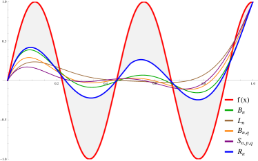
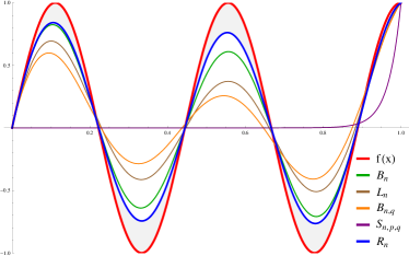
Figure 1. The approximation of $f(x)=\sin\left(\frac{9\pi}{2}x\right)$, in the case $n=10$ (left) and $n=50$ (right).

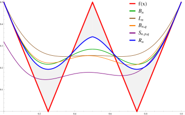
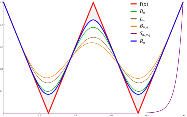
Figure 2. The approximation of $f(x)=\left|2|x-0.5|-0.5\right|$, in the case $n=10$ (left) and $n=50$ (right).

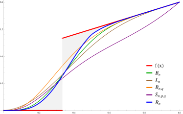
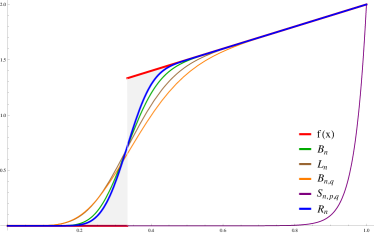
Figure 3. The approximation of $f(x)=(x+1)1_{[1/3,1]}(x)$ in the case $n=10$ (left) and $n=50$ (right).

The graphical analysis of Figures 1, 2, and 3 clearly indicates that the operator $R_{n}$ provides the best approximation of $f$ in all three cases, followed by the Bernstein operator $B_{n}$. The ranking of the remaining operators is as follows: for small values of $n$ it appears that $B_{n,q}$ provides a better approximation of $f$, while for larger values of $n$, $L_{n}$ appears to be better. Although the operator $S_{n,p,q}$ provides a reasonably good approximation of $f$ for small values of $n$, this situation changes for larger values of $n$.

References

• [1] S. N. Bernstein, Démonstration du Théorčme de Weierstrass fondée sur le calcul des Probabilités, Comm. Soc.Math. Kharkov 2 (1912), Series XIII, No.1, pp. 1 – 2.
• [2] S. Bernstein, Sur un problème du schéma des urnes á composition variable, C. R. (Doklady) Acad. Sci. URSS (N.S.) 28 (1940), pp. 5 – 7.
• [3] F. Eggenberger, G. Pólya, Über die Statistik verketteter Vorgänge, Zeitschrift Angew. Math. Mech. 3 (1923), pp. 279 – 289.
• [4] R. T. Farouki, The Bernstein polynomial basis: a centennial retrospective, Comput. Aided Geom. Design 29 (2012), No.6, pp. 379 – 419.
• [5] B. Friedman, A simple urn model, Comm. Pure Appl. Math. 2 (1949), pp. 59 – 70.
• [6] D.A. Freedman, Bernard Friedman’s urn, Ann. Math. Statist. 36 (1965), pp. 956 – 970.
• [7] S. Janson, Functional limit theorems for multitype branching processes and generalized Pólya urns, Stochastic Process. Appl. 110 (2004), No. 2, pp. 177 – 245.
• [8] N. L. Johnson, S. Kotz, Urn models and their application. An approach to modern discrete probability theory, Wiley Series in Probability and Mathematical Statistics. John Wiley & Sons, New York-London-Sydney, 1977.
• [9] A. Kajla, N. Ispir, P. N. Agrawal, M. Goyal, $q$–Bernstein–Schurer–Durrmeyer type operators for functions of one and two variables, Appl. Math. Comput. 275 (2016), pp. 372 – 385.
• [10] R. A. Khan, Some probabilistic methods in the theory of approximation operators, Acta Math. Acad. Sci. Hungar. 35 (1980), No. 1 – 2, pp. 193 – 203.
• [11] T. Kim, A note on $q$-Bernstein polynomials, Russ. J. Math. Phys. 18 (2011), No. 1, pp. 73 – 82.
• [12] G. G. Lorentz, Bernstein polynomials (second edition), Chelsea Publishing Co., New York, 1986.
• [13] L. Lupaş, A. Lupaş, Polynomials of binomial type and approximation operators, Studia Univ. Babeş-Bolyai Mathematica 32 (1987), No. 4, pp. 61 – 69.
• [14] A. Lupaş, A $q$-analogue of the Bernstein operator, Semin. Numer. Stat. Calc. Univ. Cluj-Napoca 9 (1987), pp. 85 – 92.
• [15] C. V. Muraru, Note on $q$-Bernstein-Schurer operators, Studia UBB, Mathematica LVI 2 (2011), pp. 1 – 11.
• [16] M. Mursaleen, K. J. Ansari, A. Khan, Asif, Some approximation results by $(p,q)$-analogue of Bernstein-Stancu operators, Appl. Math. Comput. 264 (2015), pp. 392 – 402.
• [17] M. N. Pascu, N. R. Pascu, Approximation properties of a new Bernstein-type operator (to appear).
• [18] T. Popoviciu, Sur l’approximation des functions convexes d’ordre supérieur, Mathematica (Cluj) 10 (1935), pp. 49 – 54.
• [19] G. Pólya, Sur quelques points de la théorie des probabilités, Ann. Inst. Poincaré 1 (1931), 117 – 161.
• [20] G. M. Phillips, On generalized Bernstein polynomials, Numerical Analysis: A. R. Mitchell 75th Birthday Volume, World Scientific, Singapore, pp. 263 – 269.
• [21] G. M. Phillips, Bernstein polynomials based on the $q$-integers,The heritage of P.L.Chebyshev, Ann. Numer. Math. 4 (1997), pp. 511 – 518.
• [22] G. M. Phillips, A survey of results on the $q$-Bernstein polynomials, IMA J. Numer. Anal. 30 (2010), No. 1, pp. 277 – 288.
• [23] F. Schurer, Linear Positive Operators in Approximation Theory, Math. Inst., Techn. Univ. Delf Report (1962).
• [24] P. C. Sikkema, Der Wert einiger Konstanten in der Theorie der Approximation mit Bernstein-Polynomen, Numer. Math. 3 (1961), pp. 107 – 116.
• [25] D. D. Stancu, Approximation of functions by a new class of linear polynomial operators, Rev. Roum. Math. Pures et Appl. 13 (1968), pp. 1173 – 1194.
• [26] V. O. Tonkov, Addition to the Popoviciu theorem, Translation of Mat. Zametki 94 (2013), No. 3, pp. 416 – 425. Math. Notes 94 (2013), No. 3 – 4, pp. 392 – 399.