1 Introduction

In 1952, A. C. Turing published the remarkable paper [36], in which a revolutionary idea about mechanism of morphogenesis (the development of structures in an organism during its life) has been proposed. From the mathematical point of view Turing’s idea immediately leads to construction of reaction-diffusion (RD) systems (not single equations!) exhibiting so called Turing instability (see, e.g., Chapter 14.3 in [25]). Nowadays nonlinear RD systems are governing equations for many well-known nonlinear second-order models used to describe various processes in biology [7, 23, 25, 27], physics [2, 33], chemistry [4], ecology [29].

At the present time, one may claim that nonlinear RD systems have been extensively studied by means of different mathematical methods, including symmetry-based (group-theoretical) methods during the last decades. However, the progress is still insufficient, in particular, Lie symmetries are not completely described for many RD systems arising in applications because of principal and technical difficulties. For example, although finding Lie symmetries of the two-component RD systems was initiated about 35 years ago [38], this Lie symmetry classification problem (the terminology ‘group classification problem’ is also used in this context) was finished only in the 2000th in papers [11, 12, 13, 28] (for constant diffusivities) and [14, 15, 22] (for nonconstant diffusivities).

In the case of nonlinear RD systems with the cross-diffusion, the problem is still open excepting the case when the system in question involves a constant cross-diffusion only [28]. Notably, Lie symmetries of some nonlinear RD systems with correctly-specified forms of cross-diffusion arising in real-world applications were studied in [10, 16, 34, 35].

In contrast to the two-component systems, the multi-component RD systems (i.e. those consisting of three and more equations) were not widely examined by symmetry-based methods. To the best of our knowledge, the most general results for the multi-component RD systems (under essential restrictions on the structure of diffusion coefficients) were derived in [15]. There are also some studies (see, e.g., [9]) devoted to the Lie symmetry search of the multi-component RD systems involving only arbitrary parameters (i.e. no any arbitrary functions as parameters). Because, a complete Lie symmetry classification of the general class of multi-component RD systems is extremely difficult problem, it it reasonable to restrict ourselves to some systems arising in real world applications.

In this paper, we examine the three-component model introduced in [3] for describing the spread of an initially localized population of farmers into a region occupied by hunter-gatherers. Under some assumptions clearly indicated in [3], the spread and interaction between farmers and hunter-gatherers can be modeled as a RD process. The corresponding nonlinear RD system has the form

$$\begin{array}[]{l}F_{t}=d_{f}F_{xx}+r_{f}F\left(1-(e_{1}F+e_{2}C)/K\right),\\ C_{t}=d_{c}C_{xx}+r_{c}C\left(1-(e_{1}F+e_{2}C)/K\right)+e_{1}FH+e_{2}CH,\\ H_{t}=d_{h}H_{xx}+r_{h}H\left(1-H/L\right)-e_{1}FH-e_{2}CH,\end{array}$$ (1)

where $F(t,x),\ C(t,x)$ and $H(t,x)$ are densities of the three populations of initial farmers, converted farmers, and hunter-gatherers, respectively. Parameters $d_{f},\ d_{c}$ and $d_{h}$ are the positive diffusion constants; $r_{f},\ r_{c}$ and $r_{h}$ are the intrinsic growth rates of initial farmers, converted farmers, and hunter-gatherers, respectively; $K$ and $L$ are the carrying capacities of farmers and hunter-gatherers; $e_{1}$ and $e_{2}$ are the conversion rates of hunter-gatherers to initial and converted farmers. Parameters $e_{2},\ r_{c}$ and $r_{h}$ are assumed to be nonnegative, while all other parameters are assumed to be positive. We note that the equalities $e_{1}=e_{2}$ and $d_{f}=d_{c}=d_{h}$ are assumed in [3]. In our opinion, it is very unlikely that the three populations of initial farmers, converted farmers, and hunter-gatherers have the same diffusivity in space, hence their diffusivities should be assumed arbitrary, i.e. the equality $d_{f}=d_{c}=d_{h}$ can take place only in a special case.

The nonlinear RDS (1) can be simplified using the following re-scaling of the variables

$$F\rightarrow\frac{K}{e_{1}}u,\ C\rightarrow\frac{KL}{r_{f}}v,\ H\rightarrow Lw,\ t\rightarrow\frac{1}{r_{f}}\,t,\ x\rightarrow\sqrt{\frac{1}{r_{f}}}\,x$$ (2)

and introducing new notation

$$a_{1}=\frac{e_{2}L}{r_{f}},\ a_{2}=\frac{r_{c}}{r_{f}},\ a_{3}=\frac{r_{h}}{r_{f}},\ a_{4}=\frac{K}{r_{f}}\neq 0,\ a_{5}=\frac{e_{2}KL}{r^{2}_{f}},\ d_{f}=d_{1},\ d_{c}=d_{2},\ d_{h}=d_{3}.$$

Re-scaling (2) in symmetry analysis is called the equivalence transformation of system (1). Transformation (2) reduce system (1) to the equivalent form

$$\begin{array}[]{l}u_{t}=d_{1}u_{xx}+u(1-u-a_{1}v),\\ v_{t}=d_{2}v_{xx}+a_{2}v(1-u-a_{1}v)+uw+a_{1}vw,\\ w_{t}=d_{3}w_{xx}+a_{3}w(1-w)-a_{4}uw-a_{5}vw.\end{array}$$ (3)

Hereafter (3) is called the hunter-gatherer–farmer (HGF) system and one is the main object of investigation in this paper. We naturally assume that $a_{4}\not=0$ (otherwise $K=0$ in (1)) and $d_{1}d_{2}d_{3}\not=0$.

The paper is organized as follows. In Section 2, the Lie symmetry classification of the HGF system (3) is derived. In Section 3, the most important (from applicability point of view) cases of system (3) with nontrivial Lie symmetries are examined. In particular, nontrivial Lie ansätze are derived and applied for reducing the systems in question to systems of ODEs. The reduced systems are analyzed in order to construct exact solutions. In Section 4, the traveling fronts (TFs) of the HGF system (3) with correctly-specified coefficients are constructed in explicit forms. The properties of TFs obtained are analysed and some biological interpretation is presented. Finally, we briefly discuss the result obtained and present some conclusions in the last section.

2 Main theorem

To find Lie invariance operators, one needs to consider system (3) as the manifold

$${\cal{M}}=\{S_{1}=0,S_{2}=0,S_{3}=0\},$$

where

$$S_{1}\equiv\ d_{1}u_{xx}-u_{t}+u(1-u-a_{1}v),$$

$$S_{2}\equiv\ d_{2}v_{xx}-v_{t}+a_{2}v(1-u-a_{1}v)+uw+a_{1}vw,$$

$$S_{3}\equiv\ d_{3}w_{xx}-w_{t}+a_{3}w(1-w)-a_{4}uw-a_{5}vw,$$

in the prolonged space of the variables

$$t,x,\ u,v,w,\ u_{t},v_{t},w_{t},u_{x},v_{x},w_{x},\ u_{xx},v_{xx},w_{xx},u_{xt},v_{xt},w_{xt},u_{tt},v_{tt},w_{tt}.$$

According to the Lie invariance criterion, system (3) is invariant under the Lie group generated by the infinitesimal operator

$$\hskip 28.45274ptX=\xi^{0}(t,x,u,v,w)\partial_{t}+\xi^{1}(t,x,u,v,w)\partial_{x}+$$

$$\eta^{1}(t,x,u,v,w)\partial_{u}+\eta^{2}(t,x,u,v,w)\partial_{v}+\eta^{3}(t,x,u,v,w)\partial_{w},$$

if the following Lie’s invariance conditions are satisfied:

$$\mbox{\raisebox{-6.88889pt}{$\stackrel{{\scriptstyle\displaystyle X}}{{\scriptstyle 2}}$}}(S_{1})\Big{|}_{\cal{M}}=0,\quad\mbox{\raisebox{-6.88889pt}{$\stackrel{{\scriptstyle\displaystyle X}}{{\scriptstyle 2}}$}}(S_{2})\Big{|}_{\cal{M}}=0,\quad\mbox{\raisebox{-6.88889pt}{$\stackrel{{\scriptstyle\displaystyle X}}{{\scriptstyle 2}}$}}(S_{3})\Big{|}_{\cal{M}}=0,$$ (4)

where the operator $\stackrel{{\scriptstyle\displaystyle X}}{{\scriptstyle 2}}$ is the second prolongation of the operator $X$ (see, e.g., [5, 6, 18, 30, 31]).

Obviously, system (3) admits the Lie algebra with the basic operators

$$P_{t}=\partial_{t},\ P_{x}=\partial_{x}$$ (5)

because one is invariant with respect to the time and space translations. It can be easily shown that (5) is the principal (trivial) algebra of system (3), i.e. this is maximal invariance algebra of this system with arbitrary coefficients $a_{j}$ and $d_{k}$. To find all possible extensions of principal algebra in the case of the system (3), one needs to apply the invariance criterion (4) and to solve the corresponding system of determining equations (DEs). Omitting rather standard calculations (nowadays they can be done using Maple, Mathematica etc.), we present the DE system obtained:

$$\xi^{0}_{x}=\xi^{0}_{u}=\xi^{0}_{v}=\xi^{0}_{w}=\xi^{1}_{u}=\xi^{1}_{v}=\xi^{1}_{w}=0,$$ (6)

$$\eta^{k}_{uu}=\eta^{k}_{uv}=\eta^{k}_{vv}=\eta^{k}_{ww}=\eta^{k}_{uw}=\eta^{k}_{vw}=0,\ k=1,2,3,$$ (7)

$$\eta^{1}_{xv}=\eta^{1}_{xw}=\eta^{2}_{xu}=\eta^{2}_{xw}=\eta^{3}_{xu}=\eta^{3}_{xv}=0,$$ (8)

$$(d_{1}-d_{2})\eta^{1}_{v}=(d_{1}-d_{3})\eta^{1}_{w}=(d_{1}-d_{2})\eta^{2}_{u}=$$

$$(d_{2}-d_{3})\eta^{2}_{w}=(d_{1}-d_{3})\eta^{3}_{u}=(d_{2}-d_{3})\eta^{3}_{v}=0,$$ (9)

$$2\xi^{1}_{x}-\xi^{0}_{t}=0,\ 2d_{1}\eta^{1}_{xu}+\xi^{1}_{t}=0,\ 2d_{2}\eta^{2}_{xv}+\xi^{1}_{t}=0,\ 2d_{3}\eta^{3}_{xw}+\xi^{1}_{t}=0,$$ (10)

$$\eta^{1}C^{1}_{u}+\eta^{2}C^{1}_{v}+\eta^{3}C^{1}_{w}+(2\xi^{1}_{x}-\eta^{1}_{u})C^{1}=\eta^{1}_{t}-d_{1}\eta^{1}_{xx}+\frac{d_{1}}{d_{2}}\,\eta^{1}_{v}C^{2}+\frac{d_{1}}{d_{3}}\,\eta^{1}_{w}C^{3},$$ (11)

$$\eta^{1}C^{2}_{u}+\eta^{2}C^{2}_{v}+\eta^{3}C^{2}_{w}+(2\xi^{1}_{x}-\eta^{2}_{v})C^{2}=\eta^{2}_{t}-d_{2}\eta^{2}_{xx}+\frac{d_{2}}{d_{1}}\,\eta^{2}_{u}C^{1}+\frac{d_{2}}{d_{3}}\,\eta^{2}_{w}C^{3},$$ (12)

$$\eta^{1}C^{3}_{u}+\eta^{2}C^{3}_{v}+\eta^{3}C^{3}_{w}+(2\xi^{1}_{x}-\eta^{3}_{w})C^{3}=\eta^{3}_{t}-d_{3}\eta^{3}_{xx}+\frac{d_{3}}{d_{1}}\,\eta^{3}_{u}C^{1}+\frac{d_{3}}{d_{2}}\,\eta^{3}_{v}C^{2},$$ (13)

where

$$\begin{array}[]{l}C^{1}=u(1-u-a_{1}v),\\ C^{2}=a_{2}v(1-u-a_{1}v)+uw+a_{1}vw,\\ C^{3}=a_{3}w(1-w)-a_{4}uw-a_{5}vw.\end{array}$$ (14)

Now we want to find all possible values of the coefficients $a_{j}$ and $d_{k}$ leading to extensions of the principal algebra (5). It means that all inequivalent solutions of the system of DEs (6)–(13) should be constructed. As a result, the following statement was proved.

Theorem 1

The HGF ystem (3) with $a_{4}d_{1}d_{2}d_{3}\not=0$ admits a nontrivial Lie algebra of symmetries if and only if one and the corresponding symmetry operators have the forms listed in Table 1.

Table 1: Lie symmetry operators of the HGF system (3)

	Reaction terms	Restrictions	Lie symmetries
1	$u(1-u)$ $a_{2}v(1-u)+uw$ $-a_{4}uw$	$a_{2}\neq 0$	$\partial_{t},\ \partial_{x},\ I=v\partial_{v}+w\partial_{w}$
2	$u(1-u)$ $uw$ $a_{3}w(1-w)-a_{4}uw$	$a_{3}\neq 0$	$\partial_{t},\ \partial_{x},$ $X^{\infty}=P(t,x)\partial_{v},$ $P_{t}=d_{2}P_{xx}$
3	$u(1-u)$ $uw$ $-a_{4}uw$		$\partial_{t},\ \partial_{x},\ I,\ X^{\infty}$
4	$u(1-u-a_{1}v)$ $v(1-u-a_{1}v)+uw+a_{1}vw$ $a_{3}w(1-w)-a_{4}uw-a_{1}a_{4}vw$	$d_{1}=d_{2}$ $a_{1}\neq 0$	$\partial_{t},\ \partial_{x},$ $Q_{1}=-a_{1}u\partial_{u}+u\partial_{v}$
5	$u(1-u)$ $v(1-u)+uw$ $a_{3}w(1-w)-a_{4}uw$	$d_{1}=d_{2}$ $a_{3}\neq 0$	$\partial_{t},\ \partial_{x},$ $u\partial_{v},\ Q_{2}=e^{t}(u-1)\partial_{v}$
6	$u(1-u)$ $v(1-u)+uw$ $-a_{4}uw$	$d_{1}=d_{2}$	$\partial_{t},\ \partial_{x},\ u\partial_{v},\ I,\ Q_{2}$
7	$u(1-u)$ $a_{4}v(1-u)+uw$ $-a_{4}uw$	$d_{2}=d_{3}$	$\partial_{t},\ \partial_{x},\ e^{a_{4}t}w\partial_{v},\ I$
8	$u(1-u)$ $uw$ $-a_{4}uw$	$d_{2}=d_{3}$	$\partial_{t},\ \partial_{x},$ $w\partial_{v}-a_{4}w\partial_{w},\ I,\ X^{\infty}$
9	$u(1-u-a_{1}v)$ $v(1-u-a_{1}v)+uw+a_{1}vw$ $-a_{4}uw-a_{1}a_{4}vw$	$d_{1}=d_{2}=d_{3}$ $a_{1}\neq 0$	$\partial_{t},\ \partial_{x},\ Q_{1},$ $e^{t}\left(\frac{a_{4}-1}{a_{1}}\,u+(a_{4}-1)v+\right.$ $\left.w+\frac{1-a_{4}}{a_{1}}\right)\left(\partial_{u}-\frac{1}{a_{1}}\partial_{v}\right)$

Continuation of Table 1

	Reaction terms	Restrictions	Lie symmetries
10	$u(1-u)$ $a_{2}v(1-u)+uw$ $-uw$	$d_{1}=d_{2}=d_{3}$ $a_{2}\neq 0,\ a_{2}\neq 1$	$\partial_{t},\ \partial_{x},\ I,$ $u\partial_{v}+(a_{2}-1)(u-1)\partial_{w}$
11	$u(1-u)$ $v(1-u)+uw$ $-uw$	$d_{1}=d_{2}=d_{3}$	$\partial_{t},\ \partial_{x},$ $u\partial_{v},\ we^{t}\partial_{v},\ I,\ Q_{2}$
12	$u(1-u)$ $uw$ $-uw$	$d_{1}=d_{2}=d_{3}$	$\partial_{t},\ \partial_{x},\ w\partial_{v}-w\partial_{w},$ $u\partial_{v}+(1-u)\partial_{w},$ $ue^{-t}(\partial_{v}-\partial_{w}),\ I,\ X^{\infty}$

Sketch of the proof. In order to prove the theorem, one needs to solve the system of DEs (6)–(13) with the functions $C^{k}\ (k=1,2,3)$ from (14). Although this is a standard routine, all possible special cases (not some of them !) should be identified and examined in order to obtain a full Lie symmetry classification.

It can be noted that the forms of the functions $\xi^{0},\ \xi^{1}$ and $\eta^{k}\ (k=1,2,3)$ can be defined independently on the functions $C^{k}$. In fact, equations (6)–(8) can be easily integrated:

$$\xi^{0}=\xi^{0}(t),\ \xi^{1}=\xi^{1}(t,x),$$

$$\eta^{1}=r^{1}(t,x)u+q^{1}(t)v+h^{1}(t)w+p^{1}(t,x),$$

$$\eta^{2}=r^{2}(t,x)v+q^{2}(t)u+h^{2}(t)w+p^{2}(t,x),$$

$$\eta^{3}=r^{3}(t,x)w+q^{3}(t)u+h^{3}(t)v+p^{3}(t,x),$$

where $\xi^{0},\ \xi^{1},\ r^{k},\ q^{k},\ h^{k}$ and $p^{k}$ ($k=1,2,3$) are to-be-determined functions.

Now we analyse equations (9). It turns out that five different cases should be examined depending on diffusion coefficients, namely: (I) $d_{k}$ are arbitrary positive constants, (II) $d_{1}=d_{2},$ (III) $d_{1}=d_{3},$ (IV) $d_{2}=d_{3}$ and (V) $d_{1}=d_{2}=d_{3}.$

Let us examine case (I). Because the diffusivities $d_{k}\ (k=1,2,3)$ are arbitrary constants, equations (9) immediately produce $q^{k}=h^{k}=0,\ k=1,2,3.$ Equations (11)–(13) can be split with respect to the variables $u,v,w$ and their products $uv,uw,vw,u^{2},$ $v^{2},w^{2}$. As a result, the system of DEs (6)–(13) reduces to the form

$$a_{1}p^{1}=0,\ p^{1}+a_{1}p^{2}=0,\ -a_{2}p^{2}+p^{3}=0,\ a_{4}p^{3}=0,\ a_{5}p^{3}=0,\ r^{2}=r^{3},$$ (15)

$$2\xi^{1}_{x}-\xi^{0}_{t}=0,r^{1}+2\xi^{1}_{x}=0,2d_{1}r^{1}_{x}+\xi^{1}_{t}=0,2d_{2}r^{2}_{x}+\xi^{1}_{t}=0,\ 2d_{3}r^{3}_{x}+\xi^{1}_{t}=0,$$ (16)

$$a_{1}(r^{2}+2\xi^{1}_{x})=0,\ a_{3}(r^{2}+2\xi^{1}_{x})=0,\ a_{5}(r^{2}+2\xi^{1}_{x})=0,$$ (17)

$$d_{1}r^{1}_{xx}-r^{1}_{t}+2\xi^{1}_{x}-2p^{1}-a_{1}p^{2}=0,$$ (18)

$$d_{2}r^{2}_{xx}-r^{2}_{t}+2a_{2}\xi^{1}_{x}-a_{2}p^{1}-2a_{1}a_{2}p^{2}+a_{1}p^{3}=0,$$ (19)

$$d_{3}r^{3}_{xx}-r^{3}_{t}+2a_{3}\xi^{1}_{x}-a_{4}p^{1}-a_{5}p^{2}-2a_{3}p^{3}=0,$$ (20)

$$d_{1}p^{1}_{xx}-p^{1}_{t}+p^{1}=0,\ d_{2}p^{2}_{xx}-p^{2}_{t}+a_{2}p^{2}=0,\ d_{3}p^{3}_{xx}-p^{3}_{t}+a_{3}p^{3}=0.$$ (21)

Because (15) is the set of algebraic equations, we find $p^{1}=p^{3}=0$ and $a_{1}a_{2}p^{2}=0,$ while the overdetermined system (16) leads to

$$\xi^{0}_{tt}=\xi^{1}_{xx}=\xi^{1}_{t}=r^{1}_{x}=r^{1}_{t}=r^{2}_{x}=0.$$

Hence, equation (18) produces $\xi^{1}_{x}=0$. Having $\xi^{1}_{x}=0$, equations (17) give $r^{2}=r^{3}=0$ provided $a_{1}^{2}+a_{3}^{2}+a_{5}^{2}\neq 0.$ In this case, one can find nontrivial Lie symmetry only under the restriction $p^{2}\neq 0$, hence $a_{1}=a_{2}=a_{5}=0.$ Thus, the general solution of (15)–(21) has the form

$$\xi^{0}=c_{0},\ \xi^{1}=c_{1},\ p^{1}=p^{3}=0,\ r^{1}=r^{2}=r^{3}=0,\ p^{2}=P(t,x)$$

(hereafter $c_{k}\ (k=0,1,\dots)$ is arbitrary constant, while the function $P(t,x)$ is an arbitrary solution of equation $P_{t}=d_{2}P_{xx}$), therefore Case 2 of Table 1 is obtained.

In the case $a_{1}=a_{3}=a_{5}=0$ we obtain Cases 1 and 3 of Table 1. Thus, case (I) is completely examined.

Now we turn to case (II). Having done a preliminary analysis, we find and

$$q^{1}=q^{3}=h^{k}=0,\ k=1,2,3,$$ (22)

$$p^{1}=p^{3}=0,\ a_{1}p^{2}=0$$

and derive the system of DEs

$$2\xi^{1}_{x}-\xi^{0}_{t}=0,\ 2d\eta^{1}_{xu}+\xi^{1}_{t}=0,\ 2d\eta^{2}_{xv}+\xi^{1}_{t}=0,\ 2d_{3}\eta^{3}_{xw}+\xi^{1}_{t}=0,$$ (23)

$$dr^{1}_{xx}-r^{1}_{t}+2\xi^{1}_{x}=0,dr^{2}_{xx}-r^{2}_{t}+2a_{2}\xi^{1}_{x}=0,d_{3}r^{3}_{xx}-r^{3}_{t}+2a_{3}\xi^{1}_{x}-a_{5}p^{2}=0,$$ (24)

$$a_{1}(r^{2}+2\xi^{1}_{x})=0,\ a_{5}(r^{2}+2\xi^{1}_{x})=0,\ a_{1}(r^{3}+2\xi^{1}_{x})=0,\ a_{3}(r^{3}+2\xi^{1}_{x})=0,$$ (25)

$$\left(-1+a_{2}\right)q^{2}=0,\ a_{1}\left(-1+2a_{2}\right)q^{2}+a_{2}\left(r^{1}+2\xi^{1}_{x}\right)=0,$$ (26)

$$a_{5}q^{2}+a_{4}\left(r^{1}+2\xi^{1}_{x}\right)=0,\ a_{1}q^{2}+r^{1}+2\xi^{1}_{x}=0,$$ (27)

$$a_{1}q^{2}+r^{1}-r^{2}+r^{3}+2\xi^{1}_{x}=0,$$ (28)

$$dq^{2}_{xx}-q^{2}_{t}+\left(a_{2}-1\right)q^{2}-a_{2}p^{2}=0,$$ (29)

$$dp^{2}_{xx}-p^{2}_{t}+a_{2}p^{2}=0$$ (30)

for finding all other functions.

It can be seen from (22) that new nontrivial Lie symmetries can exist only if $q^{2}\neq 0$ (otherwise one obtains the result of case (I)). Thus, the first equation of (26) immediately produces $a_{2}=1,$ while restriction $a_{5}=a_{1}a_{4}$ follows from the compatibility condition of equations (27).

The further analysis of the system of DEs (23)–(30) depends on the value of constant $a_{1}$.

If $a_{1}\neq 0$ then $p^{2}=0$ and $r^{2}=r^{3}=-2\xi^{1}_{x}$. As a result, equations (23) and (24) produce $r^{2}=r^{3}=0,\ r^{1}=const,\ \xi^{0}=c_{0},\ \xi^{1}=c_{1}.$ The last unknown function $q^{2}$ can be found from (27). Hence,

$$\xi^{0}=c_{0},\ \xi^{1}=c_{1},\ \eta^{1}=-a_{1}c_{3}u,\ \eta^{2}=c_{3}u,\ \eta^{3}=0,$$

and Case 4 of Table 1 is obtained. In a quite similar way, one examines the subcase $a_{1}=0$ and arrives at Cases 5–6 of Table 1.

The examination of the system of DEs in case (III) does not lead to new system of the form (3) with nontrivial Lie symmetries.

Analysis of case (IV) leads to systems and Lie symmetries listed in Cases 7 and 8 of Table 1, while case (V) produces Cases 9–12 of Table 1. The relevant calculations are omitted here.

The proof is now completed. $\square$

3 Reduction of the HGF system to ODE systems

In this section, we present examples of reductions of the HGF system (3) to ODE systems using the Lie symmetries obtained. If one compares system (3) with the reaction terms arising in Table 1 with its general form (3) then are realizes that Cases 4, 5 and 9 are the most interesting from the applicability point of view. In fact, all the other cases of Table 1 lead to the systems of the form (3) with too many zero coefficients, hence it is unlikely that such systems can describe adequately the spread and interaction between farmers and hunter-gatherers. For this reason, we consider the systems from Cases 4, 5 and 9 of Table 1 and the relevant linear combinations of the Lie symmetries involving nontrivial operators. The case of the Lie symmetry operators leading to plane wave solutions, especially TFs, is examined separately in Section 4.

First of all, we note that one diffusivity, e.g. $d_{1}$, can be set $1$ in (3) without losing a generality, hence the system from Case 4 of Table 1 have the form

$$\begin{array}[]{l}u_{t}=u_{xx}+u(1-u-a_{1}v),\ a_{1}\neq 0,\\ v_{t}=v_{xx}+v(1-u-a_{1}v)+uw+a_{1}vw,\\ w_{t}=dw_{xx}+a_{3}w(1-w)-a_{4}uw-a_{1}a_{4}vw.\end{array}$$ (31)

Let us consider two essentially different linear combinations of the Lie symmetry operators of system (31)

$$X=\partial_{t}+\alpha\partial_{x}-\beta a_{1}u\partial_{u}+\beta u\partial_{v}$$ (32)

and

$$X=\partial_{x}-\beta a_{1}u\partial_{u}+\beta u\partial_{v}.$$ (33)

Hereafter $\alpha$ and $\beta\neq 0$ are arbitrary constants.

Solving the characteristic equation

$$\frac{dt}{1}=\frac{dx}{\alpha}=\frac{du}{-\beta a_{1}u}=\frac{dv}{\beta u}$$

corresponding to operator (32) one obtains the ansatz

$$\begin{array}[]{l}u=e^{-\beta a_{1}t}U(\omega),\ \omega=x-\alpha t,\\ v=V(\omega)-\frac{1}{a_{1}}\,e^{-\beta a_{1}t}U(\omega),\\ w=W(\omega),\end{array}$$ (34)

where $U,\ V$ and $W$ are new unknown functions. Substituting ansatz (34) into (31), we arrive at the system of ODEs

$$\begin{array}[]{l}U^{\prime\prime}+\alpha U^{\prime}+U\left(1+a_{1}\beta-a_{1}V\right)=0,\\ V^{\prime\prime}+\alpha V^{\prime}+V\left(1-a_{1}V+a_{1}W\right)=0,\\ dW^{\prime\prime}+\alpha W^{\prime}+a_{3}W\left(1-W\right)-a_{1}a_{4}VW=0.\end{array}$$ (35)

One sees that the reduced system (35) is nonlinear and the problem of constructing its exact solutions is still a difficult task. However, we were able to note the three special cases

$$\mbox{(i)}\ d=a_{3}=1,\quad\mbox{(ii)}\ d=1,\ a_{3}=0,\quad\mbox{(iii)}\ d=1,\ a_{4}=1+a_{1}+a_{3},\ a_{3}\neq 0,$$

when the functions $V$ and $W$ can be found, while $U$ satisfies a separate ODE. In fact, if one assumes that the components $V$ and $W$ have the same structure as the well-known solution of the Fisher equation [1] (see formula (46) below) then the cases (i), (ii) and (iii) lead to the exact solutions

$$u=e^{-\beta a_{1}t}U(\omega),\ \omega=x-\frac{5}{\sqrt{6}}\,t,$$

$$v=\frac{1+a_{1}}{4a_{1}(1+a_{1}a_{4})}\left(1-\tanh\left[\frac{1}{2\sqrt{6}}\,\omega\right]\right)^{2}-\frac{1}{a_{1}}\,e^{-\beta a_{1}t}U(\omega),$$

$$w=\frac{1-a_{4}}{4(1+a_{1}a_{4})}\left(1-\tanh\left[\frac{1}{2\sqrt{6}}\,\omega\right]\right)^{2},$$

$$u=e^{-\beta a_{1}t}U(\omega),\ \omega=x-\frac{5\sqrt{a_{4}}}{\sqrt{6}}\,t,$$

$$v=\frac{1}{4a_{1}}\left(1-\tanh\left[\frac{\sqrt{a_{4}}}{2\sqrt{6}}\,\omega\right]\right)^{2}-\frac{1}{a_{1}}\,e^{-\beta a_{1}t}U(\omega),$$

$$w=\frac{1-a_{4}}{4a_{1}}\left(\left(1-\tanh\frac{\sqrt{a_{4}}}{2\sqrt{6}}\,\omega\right)^{2}-4\right)$$

and

$$u=e^{-\beta a_{1}t}U(\omega),\ \omega=x-\frac{5\sqrt{1+a_{1}}}{\sqrt{6}}\,t,$$

$$v=\frac{1}{4a_{1}}\left(1-\tanh\left[\frac{\sqrt{1+a_{1}}}{2\sqrt{6}}\,\omega\right]\right)^{2}-\frac{1}{a_{1}}\,e^{-\beta a_{1}t}U(\omega),$$

$$w=1-\frac{1}{4}\left(1-\tanh\frac{\sqrt{1+a_{1}}}{2\sqrt{6}}\,\omega\right)^{2},$$

respectively. Here the function $U$ is an arbitrary solution of the linear ODE

$$U^{\prime\prime}+\alpha U^{\prime}+U\left(1+a_{1}\beta-\kappa_{1}\left(1-\tanh\left[\frac{\kappa_{2}}{2\sqrt{6}}\,\omega\right]\right)^{2}\right)=0,$$ (36)

where

$$\kappa_{1}=\left\{\begin{array}[]{l}\frac{1+a_{1}}{4(1+a_{1}a_{4})}\hskip 11.38092pt\mbox{in case (i)},\\ \frac{1}{4}\hskip 45.52458pt\mbox{in case (ii)},\\ \frac{1}{4}\hskip 45.52458pt\mbox{in case (iii)},\end{array}\right.\quad\kappa_{2}=\left\{\begin{array}[]{l}1\hskip 45.52458pt\mbox{in case (i)},\\ \sqrt{a_{4}}\hskip 31.2982pt\mbox{in case (ii)},\\ \sqrt{1+a_{1}}\hskip 14.22636pt\mbox{in case (iii)}.\end{array}\right.$$

Ansatz corresponding to operator (33) and the reduced system for system (31) have the forms

$$\begin{array}[]{l}u=U(t)e^{-\beta a_{1}x},\quad v=V(t)-\frac{e^{-\beta a_{1}x}}{a_{1}}\,U(t),\quad w=W(t)\end{array}$$ (37)

and

$$\begin{array}[]{l}U^{\prime}+U(a_{1}V-1-\beta^{2}a_{1}^{2})=0,\\ V^{\prime}+V(a_{1}V-a_{1}W-1)=0,\\ W^{\prime}+W(a_{3}W+a_{1}a_{4}V-a_{3})=0.\end{array}$$ (38)

We have solved system (38) assuming that the functions $V$ and $W$ are linearly dependent. In a such way three different cases

$$\mbox{(i)}\ a_{3}=1,\quad\mbox{(ii)}\ a_{3}=0,\quad\mbox{(iii)}\ a_{4}=1+a_{1}+a_{3},\ a_{3}\neq 0$$

hold. Thus the cases (i), (ii) and (iii) lead to the exact solutions

$$\begin{array}[]{l}U=\frac{\delta_{2}e^{(1+\beta^{2}a_{1}^{2})t}}{\left(1-\delta_{1}+\delta_{1}e^{t}\right)^{\frac{1+a_{1}}{1+a_{1}a_{4}}}},\quad V=\frac{1+a_{1}}{a_{1}(1+a_{1}a_{4})}\frac{\delta_{1}e^{t}}{1-\delta_{1}+\delta_{1}e^{t}},\quad W=\frac{1-a_{4}}{1+a_{1}a_{4}}\frac{\delta_{1}e^{t}}{1-\delta_{1}+\delta_{1}e^{t}},\end{array}$$ (39)

$$U=\frac{\delta_{2}e^{(1+\beta^{2}a_{1}^{2})t}}{\left(1-\delta_{1}+\delta_{1}e^{a_{4}t}\right)^{\frac{1}{a_{4}}}},\ V=\frac{\delta_{1}e^{a_{4}t}}{a_{1}\left(1-\delta_{1}+\delta_{1}e^{a_{4}t}\right)},\ W=\frac{(1-a_{4})(\delta_{1}-1)}{a_{1}\left(1-\delta_{1}+\delta_{1}e^{a_{4}t}\right)}$$

and

$$U=\frac{\delta_{2}e^{(1+\beta^{2}a_{1}^{2})t}}{\left(1-\delta_{1}+\delta_{1}e^{(1+a_{1})t}\right)^{\frac{1}{1+a_{1}}}},\ V=\frac{\delta_{1}e^{(1+a_{1})t}}{a_{1}\left(1-\delta_{1}+\delta_{1}e^{(1+a_{1})t}\right)},\ W=\frac{1-\delta_{1}}{1-\delta_{1}+\delta_{1}e^{(1+a_{1})t}}$$

(here $\delta_{1}$ and $\delta_{2}$ are arbitrary positive constants) of system (38), respectively.

Let us consider the most interesting solution (39) from the applicability point of view in detail. Substituting (39) into ansatz (37), the three-parameter family of exact solutions

$$\begin{array}[]{l}u=\frac{\delta_{2}\exp\left((1+\beta^{2}a_{1}^{2})t-\beta a_{1}x\right)}{\left(1-\delta_{1}+\delta_{1}e^{t}\right)^{\frac{1+a_{1}}{1+a_{1}a_{4}}}},\\ v=\frac{1+a_{1}}{a_{1}(1+a_{1}a_{4})}\frac{\delta_{1}e^{t}}{1-\delta_{1}+\delta_{1}e^{t}}-\frac{\delta_{2}\exp\left((1+\beta^{2}a_{1}^{2})t-\beta a_{1}x\right)}{a_{1}\left(1-\delta_{1}+\delta_{1}e^{t}\right)^{\frac{1+a_{1}}{1+a_{1}a_{4}}}},\\ w=\frac{1-a_{4}}{1+a_{1}a_{4}}\frac{\delta_{1}e^{t}}{1-\delta_{1}+\delta_{1}e^{t}}\end{array}$$ (40)

of system (31) with $a_{3}=1$ is obtained.

It can be noted that the components of exact solutions of the form (40) are nonnegative on the space interval $x\in(0,+\infty)$ provided the restrictions

$$\beta=\sqrt{\frac{1-a_{4}}{a_{1}(1+a_{1}a_{4})}},\ a_{4}<1,\ \delta_{1}>1,\ \delta_{2}<\frac{1+a_{1}}{1+a_{1}a_{4}}$$ (41)

hold. In this case, the solutions possess the asymptotical behaviour

$$u\rightarrow\delta_{2}\delta_{1}^{-\frac{1+a_{1}}{1+a_{1}a_{4}}}e^{-\beta a_{1}x},\ v\rightarrow\frac{1+a_{1}}{a_{1}(1+a_{1}a_{4})}-\frac{\delta_{2}}{a_{1}}\,\delta_{1}^{-\frac{1+a_{1}}{1+a_{1}a_{4}}}e^{-\beta a_{1}x},\ w\rightarrow\frac{1-a_{4}}{1+a_{1}a_{4}}$$ (42)

as $t\rightarrow\infty.$

Such behaviour predicts the scenario when the populations of initial farmers, converted farmers, and hunter-gatherers coexist in space-time, moreover the distribution of two populations is inhomogeneous as $t\rightarrow\infty$. Notably, this scenario occurs at any semi-finite interval (instead of the fixed interval $(0,+\infty)$) because system (31) is invariant with respect to the space translations.

The system and the most general linear combinations of the Lie symmetries from Case 5 of Table 1 have the forms

$$\begin{array}[]{l}u_{t}=u_{xx}+u(1-u),\\ v_{t}=v_{xx}+v(1-u)+uw,\\ w_{t}=dw_{xx}+a_{3}w(1-w)-a_{4}uw\end{array}$$ (43)

and

$$X=\partial_{t}+\alpha\partial_{x}+\beta u\partial_{v}+\gamma e^{t}(u-1)\partial_{v},$$ (44)

$$X=\partial_{x}+\beta u\partial_{v}+\gamma e^{t}(u-1)\partial_{v}.$$ (45)

As one can see, the first equation of system (43) is the famous Fisher equation [17] that is not integrable. There were many attempts to construct its exact solutions taking into account some reasonable initial and boundary conditions. In particular, the appropriate exact solution in the form of the TF

$$u\equiv U(\omega)=\frac{1}{4}\left(1-\tanh\left[\frac{1}{2\sqrt{6}}\,\omega\right]\right)^{2},\quad\omega=x-\frac{5}{\sqrt{6}}\,t$$ (46)

was found in [1]. We remind the reader that a plane wave solution of a PDE, which is nonnegative, bounded and satisfies the zero Neumann conditions at infinity, is usually called TF.

Ansatz corresponding to (44) and the reduced system for system (43) have the forms

$$u=U(\omega),\ \omega=x-\alpha t,$$

$$v=V(\omega)+\left(\beta t+\gamma e^{t}\right)U(\omega)-\gamma e^{t},$$

$$w=W(\omega)$$

and

$$\begin{array}[]{l}U^{\prime\prime}+\alpha U^{\prime}+U(1-U)=0,\\ V^{\prime\prime}+\alpha V^{\prime}+V(1-U)+U\left(W-\beta\right)=0,\\ dW^{\prime\prime}+\alpha W^{\prime}+a_{3}W(1-W)-a_{4}UW=0.\end{array}$$ (47)

It can be noted that the last equation of system (47) with the function $U$ from (46) has the solutions

$$W=\frac{1-a_{4}}{4}\left(1-\tanh\left[\frac{1}{2\sqrt{6}}\,\omega\right]\right)^{2},$$ (48)

if $d=a_{3}=1$ and

$$W=1-\frac{1}{4}\left(1-\tanh\left[\frac{1}{2\sqrt{6}}\,\omega\right]\right)^{2},$$ (49)

if $d=1,\ a_{4}=1+a_{3}.$

Thus, we obtain the solutions of the HGF system (43) in the forms

$$\begin{array}[]{l}u=\frac{1}{4}\left(1-\tanh\left[\frac{1}{2\sqrt{6}}\,\omega\right]\right)^{2},\ \omega=x-\frac{5}{\sqrt{6}}\,t,\\ v=V(\omega)+\frac{1}{4}\left(\beta t+\gamma e^{t}\right)\left(1-\tanh\left[\frac{1}{2\sqrt{6}}\,\omega\right]\right)^{2}-\gamma e^{t},\\ w=\frac{1-a_{4}}{4}\left(1-\tanh\left[\frac{1}{2\sqrt{6}}\,\omega\right]\right)^{2},\end{array}$$ (50)

if $d=a_{3}=1$ and

$$\begin{array}[]{l}u=\frac{1}{4}\left(1-\tanh\left[\frac{1}{2\sqrt{6}}\,\omega\right]\right)^{2},\ \omega=x-\frac{5}{\sqrt{6}}\,t,\\ v=V(\omega)+\frac{1}{4}\left(\beta t+\gamma e^{t}\right)\left(1-\tanh\left[\frac{1}{2\sqrt{6}}\,\omega\right]\right)^{2}-\gamma e^{t},\\ w=1-\frac{1}{4}\left(1-\tanh\left[\frac{1}{2\sqrt{6}}\,\omega\right]\right)^{2}\end{array}$$ (51)

if $d=1,\ a_{4}=1+a_{3}.$ In (50) and (51), the function $V$ is an arbitrary solution of the linear ODE

$$V^{\prime\prime}+\alpha V^{\prime}+V(1-U)+U\left(W-\beta\right)=0$$ (52)

with $W$ from (48) and (49), respectively, while $U$ is given by formula (46).

Remark 1

Although ODEs (36) and (52) are linear, we were unable to solve them exactly and they are not listed in the well-known handbooks like [21, 32].

Ansatz corresponding to operator (45) have the form

$$\begin{array}[]{l}u=U(t),\quad v=V(t)+\left(\beta t+\gamma e^{t}\right)x\,U(t)-\gamma e^{t}x,\quad w=W(t).\end{array}$$ (53)

Note that the exact solutions of the form (53) are not important from the applicability point of view because two components ($u$ and $w$) depend only on the variable $t$.

Table 2:

Operator	Ansatz	Reduced system
(55) with $1+\beta a_{1}\neq 0$	$u=e^{-\beta a_{1}t}U(\omega)+\frac{\gamma e^{t}}{1+\beta a_{1}}\left((a_{4}-1)V(\omega)+\right.$ $\left.W(\omega)+(1-a_{4})/a_{1}\right),\ \omega=x-\alpha t,$ $v=V(\omega)-\frac{u}{a_{1}},$ $w=W(\omega)$	$U^{\prime\prime}+\alpha U^{\prime}+U\left(1+a_{1}\beta-a_{1}V\right)=0,$ $V^{\prime\prime}+\alpha V^{\prime}+V\left(1-a_{1}V+a_{1}W\right)=0,$ $W^{\prime\prime}+\alpha W^{\prime}-a_{1}a_{4}VW=0$
(55) with $1+\beta a_{1}=0$	$u=e^{t}\left(U(\omega)+\gamma\left((a_{4}-1)V(\omega)+\right.\right.$ $\left.\left.W(\omega)+(1-a_{4})/a_{1}\right)t\right),\ \omega=x-\alpha t,$ $v=V(\omega)-\frac{u}{a_{1}},$ $w=W(\omega)$	$U^{\prime\prime}+\alpha U^{\prime}-a_{1}UV-$ $\gamma\left((a_{4}-1)V+W+(1-a_{4})/a_{1}\right)=0,$ $V^{\prime\prime}+\alpha V^{\prime}+V\left(1-a_{1}V+a_{1}W\right)=0,$ $W^{\prime\prime}+\alpha W^{\prime}-a_{1}a_{4}VW=0,$
(56) with $\beta\neq 0$	$u=e^{-\beta a_{1}x}U(t)+\frac{\gamma e^{t}}{\beta a_{1}}((a_{4}-1)V(t)+$ $W(t)+(1-a_{4})/a_{1}),$ $v=V(t)-\frac{u}{a_{1}},$ $w=W(t)$	$U^{\prime}+U\left(a_{1}V-1-a_{1}^{2}\beta^{2}\right)=0,$ $V^{\prime}+V\left(a_{1}V-a_{1}W-1\right)=0,$ $W^{\prime}+a_{1}a_{4}VW=0,$
(56) with $\beta=0$	$u=U(t)+\gamma e^{t}((a_{4}-1)V(t)+$ $W(t)+(1-a_{4})/a_{1})x,$ $v=V(t)-\frac{u}{a_{1}},$ $w=W(t)$	$U^{\prime}+U\left(a_{1}V-1\right)=0,$ $V^{\prime}+V\left(a_{1}V-a_{1}W-1\right)=0,$ $W^{\prime}+a_{1}a_{4}VW=0,$

Finally, we examine the HGF system

$$\begin{array}[]{l}u_{t}=u_{xx}+u(1-u-a_{1}v),\ a_{1}\neq 0,\\ v_{t}=v_{xx}+v(1-u-a_{1}v)+uw+a_{1}vw,\\ w_{t}=w_{xx}-a_{4}uw-a_{1}a_{4}vw,\end{array}$$ (54)

corresponding to Case 9 of Table 1. The most general linear combinations of its Lie symmetries

$$\begin{array}[]{l}\hskip 28.45274ptX=\partial_{t}+\alpha\partial_{x}+\beta(-a_{1}u\partial_{u}+u\partial_{v})+\\ \gamma e^{t}\left(\frac{a_{4}-1}{a_{1}}\,u+(a_{4}-1)v+w+\frac{1-a_{4}}{a_{1}}\right)\left(\partial_{u}-\frac{1}{a_{1}}\partial_{v}\right)\end{array}$$ (55)

and

$$\begin{array}[]{l}\hskip 28.45274ptX=\partial_{x}+\beta(-a_{1}u\partial_{u}+u\partial_{v})+\\ \gamma e^{t}\left(\frac{a_{4}-1}{a_{1}}\,u+(a_{4}-1)v+w+\frac{1-a_{4}}{a_{1}}\right)\left(\partial_{u}-\frac{1}{a_{1}}\partial_{v}\right)\end{array}$$ (56)

lead to the ansätze and the reduced systems for system (54) presented in Table 2.

4 Traveling wave solutions and their interpretation

In this section, we look for TFs (a special subclass of the plane wave solutions) of the HGF system (3). TFs are the most common in theoretical and applied studies of nonlinear real world models (see, e.g., [7, 25, 26, 27]). In the case of a single RD equation, a substantial number of such solutions are presented in [19]. Although paper [3] devoted to study TFs of system (1), such solutions are not explicitly presented therein. Here we construct several TFs of the HGF system (3) and present their interpretation.

As we noted above, one diffusivity can be set $1$ in (3) without losing a generality, hence we consider system

$$\begin{array}[]{l}u_{t}=u_{xx}+u(1-u-a_{1}v),\\ v_{t}=d_{2}v_{xx}+a_{2}v(1-u-a_{1}v)+uw+a_{1}vw,\\ w_{t}=d_{3}w_{xx}+a_{3}w(1-w)-a_{4}uw-a_{5}vw\end{array}$$ (57)

in what follows. Because system (57) with arbitrary coefficienrs admits only the trivial algebra (5), the plane wave ansatz

$$u=U(\omega),\ \omega=x-\alpha t,\ v=V(\omega),\ w=W(\omega)$$

can be easily derived, which reduces (57) to the nonlinear ODE system

$$\begin{array}[]{l}U^{\prime\prime}+\alpha U^{\prime}+U(1-U-a_{1}V)=0,\\ d_{2}V^{\prime\prime}+\alpha V^{\prime}+a_{2}V(1-U-a_{1}V)+UW+a_{1}VW=0,\\ d_{3}W^{\prime\prime}+\alpha W^{\prime}+a_{3}W(1-W)-a_{4}UW-a_{5}VW=0.\end{array}$$ (58)

Obviously, the ODE system (58) with arbitrary coefficients is not integrable, hence, we seek for its particular solutions. Our aim is to find TFs, i.e. such plane wave solutions, which are positive and bounded for arbitrary $x$ and $t>0$. Moreover, in order to provide a biological interpretation of determined solutions, we assume that the solutions to-be-determined connect the steady-state points of system (57). Taking into account the arguments presented above, we consider the ad hoc ansatz

$$\begin{array}[]{l}U=\sigma_{1}\left(1-\tanh\mu\,\omega\right)^{k_{1}},\\ V=\sigma_{2}\left(1-\tanh\mu\,\omega\right)^{k_{2}},\\ W=1-\sigma_{3}\left(1-\tanh\mu\,\omega\right)^{k_{3}}.\end{array}$$ (59)

Notably, ansätze of such form are often used and the corresponding technique is often called the tanh method [24, 37].

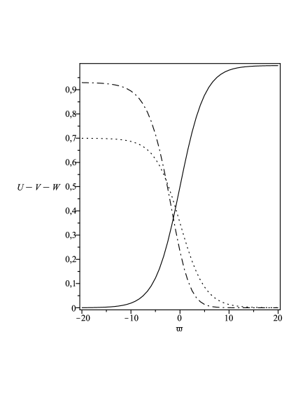
Figure 1: Curves representing the functions $U(\omega)$ (dash-dot), $V(\omega)$ (dot) and $W(\omega)$ (solid) from (60) for parameters $a_{1}=1/10$ and $\delta=7/20$.

We assume that the exact solution of the form (59) connects steady-state points of (58), namely $(U_{0},V_{0},0)$ (as $\omega\rightarrow-\infty$) and $(0,0,1)$ (as $\omega\rightarrow+\infty$). Having such assumption, one immediately obtains the restrictions

$$1-2^{k_{1}}\sigma_{1}-a_{1}2^{k_{2}}\sigma_{2}=0,\ 1-2^{k_{3}}\sigma_{3}=0.$$

Substituting ansatz (59) into (58) and making the corresponding calculations, the exact solution

$$\begin{array}[]{l}U=\frac{1}{4}(1-2a_{1}\delta)\left(1-\tanh\left[\frac{\sqrt{1-2a_{1}\delta}}{2\sqrt{6}}\,\omega\right]\right)^{2},\\ V=\delta-\delta\tanh\left[\frac{\sqrt{1-2a_{1}\delta}}{2\sqrt{6}}\,\omega\right],\\ W=\frac{1}{2}+\frac{1}{2}\tanh\left[\frac{\sqrt{1-2a_{1}\delta}}{2\sqrt{6}}\,\omega\right]\end{array}$$ (60)

of system (58) was constructed. Here $a_{1}\leq\frac{1}{2\delta}$ (otherwise the solution is complex), $\delta>0$ (otherwise $V$ is negative) and the additional restrictions

$$\begin{array}[]{l}\vskip 6.0pt plus 2.0pt minus 2.0pt\alpha=\frac{5-4a_{1}\delta}{\sqrt{6-12a_{1}\delta}},\ d_{2}=\frac{-3-5\delta+6a_{1}\delta+4a_{1}\delta^{2}}{\delta(-3+2a_{1}\delta)},\ a_{2}=\frac{3-10\delta+6a_{1}\delta+8a_{1}\delta^{2}}{6\delta(-3+2a_{1}\delta)},\\ \hskip 56.9055pta_{4}=\frac{d_{3}}{3},\ a_{5}=\frac{5-d_{3}+6a_{3}-4a_{1}\delta+2a_{1}d_{3}\delta}{12\delta}\end{array}$$ (61)

must take place. Because $d_{2}>0,\ a_{2}\geq 0$ and $a_{5}\geq 0$, the further restrictions

$$\begin{array}[]{l}a_{3}\leq\frac{1}{6}\left(-5+4\delta a_{1}+d_{3}-2\delta a_{1}d_{3}\right),\ d_{3}\geq\frac{5-4\delta a_{1}}{1-2\delta a_{1}},\\ a_{1}\leq\left\{\begin{array}[]{l}\frac{1}{2\delta},\ \mbox{if}\ \delta>1,\\ \frac{-3+10\delta}{2\delta(3+4\delta)},\ \mbox{if}\ \frac{3}{10}\leq\delta\leq 1\end{array}\right.\end{array}$$ (62)

are obtain from (61).

As one can see, the exact solution (60) is nothing else but the exact solution connecting the steady-state points $\left(1-2a_{1}\delta,2\delta,0\right)$ and $(0,0,1)$ of system (58), because

$$(U,V,W)\rightarrow\left(1-2a_{1}\delta,2\delta,0\right)\ \mbox{if}\ \omega\rightarrow-\infty,$$

$$(U,V,W)\rightarrow(0,0,1)\ \mbox{if}\ \omega\rightarrow+\infty.$$

An example of the exact solution (60) is presented in Fig. 1.

Thus, the one-parameter family of TFs

$$\begin{array}[]{l}u=\frac{1}{4}(1-2a_{1}\delta)\left(1-\tanh\left[\frac{\sqrt{1-2a_{1}\delta}}{2\sqrt{6}}(x-\alpha t)\right]\right)^{2},\\ v=\delta-\delta\tanh\left[\frac{\sqrt{1-2a_{1}\delta}}{2\sqrt{6}}(x-\alpha t)\right],\\ w=\frac{1}{2}+\frac{1}{2}\tanh\left[\frac{\sqrt{1-2a_{1}\delta}}{2\sqrt{6}}(x-\alpha t)\right]\end{array}$$ (63)

of the HGF system (57) with restrictions (61)–(62) is derived. This solution has a clear biological interpretation and describes such interaction between farmers and hunter-gatherers that hunter-gatherers die while the initial and converted farmers coexist (see Fig. 2). Actually, one may say that extinction of hunter-gatherers takes place because all of them are converted into farmers.

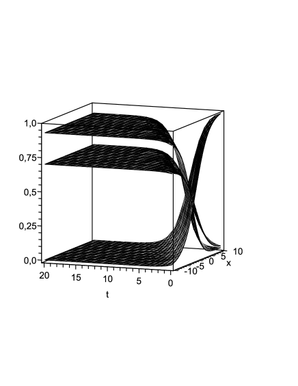
Figure 2: Surfaces representing TF (63) with $\alpha=81/5\sqrt{62}$ and $\delta=7/20$ of the HGF system (57) with the parameters $a_{1}=1/10,\ a_{2}=64/2051,\ a_{4}=d_{3}/3,\ a_{5}=(162+200a_{3}-31d_{3})/140,\ d_{2}=8982/2051$.

Now we turn to system (57) with $a_{1}=0$:

$$\begin{array}[]{l}u_{t}=u_{xx}+u(1-u),\\ v_{t}=d_{2}v_{xx}+a_{2}v(1-u)+uw,\\ w_{t}=d_{3}w_{xx}+a_{3}w(1-w)-a_{4}uw-a_{5}vw.\end{array}$$ (64)

It follows from Theorem 1 that system (64) with $a_{2}\neq 0$ and $a_{3}+a_{5}>0$ admits only the trivial algebra (5).

In order to construct exact solution of system (64), an analog of ad hoc ansatz (59) and additional restrictions have been again used. As a result, TF

$$\begin{array}[]{l}u(t,x)\equiv U(\omega)=\frac{1}{4}\left(1-\tanh\left[\frac{1}{2\sqrt{6}}\,\omega\right]\right)^{2},\ \omega=x-\frac{5}{\sqrt{6}}\,t,\\ v(t,x)\equiv V(\omega)=\frac{3d-5}{3(d-5)}\left(1-\tanh\left[\frac{1}{2\sqrt{6}}\,\omega\right]\right)^{3},\\ w(t,x)\equiv W(\omega)=\frac{3d-5}{2(d-5)}\left(1-\tanh^{2}\left[\frac{1}{2\sqrt{6}}\,\omega\right]\right)\end{array}$$ (65)

of the system

$$u_{t}=u_{xx}+u(1-u),$$

$$v_{t}=\frac{1}{2}\,v_{xx}+v(1-u)+uw,$$

$$w_{t}=dw_{xx}+\frac{5-d}{6}\,w(1-w)-\frac{5}{3}\,uw$$

was constructed (here $d\leq 5/3$).

TF (65) connects the steady-state points $\left(1,\frac{8(3d-5)}{3(d-5)},0\right)$ and $(0,0,0)$ because

$$(U,V,W)\rightarrow\left(1,\frac{8(3d-5)}{3(d-5)},0\right)\ \mbox{if}\ \omega\rightarrow-\infty,$$

$$(U,V,W)\rightarrow(0,0,0)\ \mbox{if}\ \omega\rightarrow+\infty.$$

Thus, the biological interpretation of solution (65) is similar to that for solution (63). Notably, TF (65) in contrast to that (63) has the fixed wave velocity $\alpha=\frac{5}{\sqrt{6}},$ which is exactly the same as for TF (46) of the Fisher equation.

Remark 2

Because the HGF system (3) is invariant with respect to the discrete transformation $x\rightarrow-x$, all the solutions obtained above can be transformed to another solutions using this transformation.

5 Conclusions

In this paper, the three-component nonlinear system of PDEs (1) introduced in [3] for describing the spread of an initially localized population of farmers into a region occupied by hunter-gatherers was studied by the classical Lie method. First of all the system was transformed to the nondimensional form (2) in order to reduce the number of parameters. All possible Lie symmetries of system (2) were identified (Theorem1), inequivalent symmetry reductions to the ODE systems in the most interesting case (from applicability point of view) were conducted (Section 3), several families of exact solutions (including the travelling fronts) were found and a possible biological interpretation for some of them was provided (Section 4).

It is worth noting that the nonlinear system (1) was studied under the restriction $e_{1}\not=0$, otherwise the system reduces to the three-component diffusive Lotka–Volterra system (DLVS). Lie symmetries of the three-component DLVS are completely described in [9], while its exact solutions were constructed in [9, 8, 20].

To the best of our knowledge, this paper is the first study of the HGF model by symmetry-based methods. In [3], the authors studied the existence and behaviour of TFs of the model, however any exact solutions are not presented therein. In particular, it is stated that there are TFs connecting the stable and unstable steady-state points of the model (see P.10 in [3]). Interestingly that TF (63) corresponds exactly to such case provided restrictions (61)–(62) hold. Moreover, we constructed the exact solution (40), which predicts coexistence of all the populations at any semifinal space interval (see formulae (42)) provided the coefficients of the HGF system (3) satisfy the restrictions (41). Such type of behaviour was not identified in [3].

A natural continuation of this research is searching for non-Lie (nonclassical, conditional, etc.) symmetries of the nonlinear system (1) and their application for constructing exact solutions. We have achieved some progress in this direction and plan to report new results in a forthcoming paper.

References

• [1] Ablowitz, M. & Zeppetella, A. (1979) Explicit solutions of Fisher’s equation for a special wave speed. Bull. Math. Biol. 41, 835–840.
• [2] Ames, W.F. (1972) Nonlinear partial differential equations in engineering. New York. Academic Press.
• [3] Aoki, K., Shida, M. & Shigesada, N. (1996) Travelling wave solutions for the spread of farmers into a region occupied by hunter-gatherers. Theor. Popul. Biol. 50, 1–17.
• [4] Aris, R. (1975) The Mathematical Theory of the Diffusion and Reaction in Permeable Catalysts. Vol. I, II. Oxford. Oxford University Press.
• [5] Arrigo, D.J. (2015) Arrigo, D.J.: Symmetry Analysis of Differential Equations. Hoboken, NJ. John Wiley & Sons, Inc.
• [6] Bluman, G. W., Cheviakov, A. F. & Anco, S. C. (2010) Applications of symmetry methods to partial differential equations. New York. Springer.
• [7] Britton, N. F. (2003) Essential mathematical biology. Berlin. Springer.
• [8] Chen, C.-C., Hung, L.-C. (2012) Exact travelling wave solutions of three-species competition-diffusion systems. Discrete Contin. Dyn. Syst. Ser. B. 17, 2653–2669.
• [9] Cherniha, R. & Davydovych, V. (2013) Lie and conditional symmetries of the three-component diffusive Lotka–Volterra system. J. Phys. A: Math. Theor. 46, 185204 (14 pp).
• [10] Cherniha, R., Davydovych, V. & Muzyka, L. (2017) Lie symmetries of the Shigesada–Kawasaki–Teramoto system. Comm. Nonlinear Sci. Numer. Simulat. 45 81–92.
• [11] Cherniha, R., King, J. R. (2000) Lie symmetries of nonlinear multidimensional reaction-diffusion systems: I. J. Phys. A: Math. Gen. 33, 267–282.
• [12] Cherniha, R., King, J. R. (2000) Addendum: “Lie symmetries of nonlinear multidimensional reaction-diffusion systems: I”. J. Phys. A: Math. Gen. 33, 7839–7841.
• [13] Cherniha, R., King, J. R. (2003) Lie symmetries of nonlinear multidimensional reaction-diffusion systems: II. J. Phys. A: Math. Gen. 36, 405–425.
• [14] Cherniha, R., King, J. R. (2005) Nonlinear reaction-diffusion systems with variable diffusivities: Lie symmetries, ansätze and exact solutions. J. Math. Anal. Appl. 308, 11–35.
• [15] Cherniha, R., King, J. R. (2006) Lie symmetries and conservation laws of nonlinear multidimensional reaction-diffusion systems with variable diffusivities. IMA J. Appl. Math. 71, 391–408.
• [16] Cherniha, R. M. & Wilhelmsson, H. (1996) Symmetry and exact solution of heat-mass transfer equations in thermonuclear plasma. Ukr. Math. J. 48, 1434–1449.
• [17] Fisher, R. A. (1937) The wave of advance of advantageous genes. Ann. Eugenics. 7, 353–369.
• [18] Fushchych, W. I., Shtelen, W. M. & Serov, M. I. (1993) Symmetry analysis and exact solutions of equations of nonlinear mathematical physics. Dordrecht. Kluwer.
• [19] Gilding, B. H. & Kersner, R. (2004) Travelling waves in nonlinear reaction–convection–diffusion. Basel. Birkhauser Verlag.
• [20] Hung, L.-C. (2011) Traveling wave solutions of competitive–cooperative Lotka–Volterra systems of three species. Nonlinear Anal. Real World Appl. 12, 3691–3700.
• [21] Kamke, E. (1977) Differentialgleichungen. Lösungsmethoden und Lösungen. I: Gewöhnliche (in German). Stuttgart.
• [22] Knyazeva, I. V. & Popov, M. D. (1994) A system of two diffusion equations. CRC Handbook of Lie group analysis of differential equations. CRC Press, Boca Raton 1, 171–176.
• [23] Kuang, Y., Nagy, J. D. & Eikenberry, S. E. (2016) Introduction to mathematical oncology. Boca Raton. CRC Press Company.
• [24] Malfliet, W. (2004) The tanh method: a tool for solving certain classes of nonlinear evolution and wave equations. J. Comp. Appl. Math. 164, 529–541.
• [25] Murray, J. D. (1989) Mathematical biology. Berlin. Springer.
• [26] Murray, J. D. (2003) An Introduction I: models and biomedical applications. Berlin. Springer.
• [27] Murray, J. D. (2003) Mathematical biology II: spatial models and biomedical applications. Berlin. Springer.
• [28] Nikitin, A. G (2005) Group classification of systems of nonlinear reaction-diffusion equations. Ukr. Math. Bull. 2, 153–204.
• [29] Okubo, A. & Levin, S. A. (2001) Diffusion and ecological problems. Modern Perspectives, 2nd edn. Berlin. Springer.
• [30] Olver, P. (1986) Applications of Lie groups to differential equations. Berlin. Springer.
• [31] Ovsiannikov, L. V. (1980) The group analysis of differential equations. New York. Academic Press.
• [32] Polyanin, A. D. & Zaitsev, V. F. (2003) Handbook of exact solutions for ordinary differential equations. London. CRC Press Company.
• [33] Samarskii, A. A., Galaktionov, V. A., Kurdyumov, S. P. & Mikhailov, A. P. (1995) Blow-up in quasilinear parabolic equations. Berlin. Walter de Gruyter.
• [34] Serov, M. & Omelian, O. (2008) Classification of the symmetry properties of a system of chemotaxis equations. Ukr. Math. Bull. 5, 529–557.
• [35] Torrisi, M., Tracina, R. & Valenti, A. (1996) A group analysis approach for a non linear differential system arising in diffusion phenomena. J. Math. Phys. 37, 4758–4767.
• [36] Turing, A. M. (1952) The chemical basis of morphogenesis. Phil. Trans. Roy. Soc. London 237, 37–72.
• [37] Wazwaz, A. M. (2008) The extended tanh method for the Zakharo–Kuznetsov (ZK) equation, the modified ZK equation, and its generalized forms. Commun. Nonlinear Sci. Numer. Simulat. 13, 1039–1047.
• [38] Zulehner, W. & Ames, W. F. (1983) Group analysis of a semilinear vector diffusion equation. Nonlinear Anal. 7, 945–969.