EagleMine: Vision-Guided Mining in Large Graphs

Abstract

Given a graph with millions of nodes, what patterns exist in the distributions of node characteristics, and how can we detect them and separate anomalous nodes in a way similar to human vision? In this paper, we propose a vision-guided algorithm, EagleMine, to summarize micro-cluster patterns in two-dimensional histogram plots constructed from node features in a large graph. EagleMine utilizes a water-level tree to capture cluster structures according to vision-based intuition at multi-resolutions. EagleMine traverses the water-level tree from the root and adopts statistical hypothesis tests to determine the optimal clusters that should be fitted along the path, and summarizes each cluster with a truncated Gaussian distribution. Experiments on real data show that our method can find truncated and overlapped elliptical clusters, even when some baseline methods split one visual cluster into pieces with Gaussian spheres. To identify potentially anomalous micro-clusters, EagleMine also a designates score to measure the suspiciousness of outlier groups (i.e. node clusters) and outlier nodes, detecting bots and anomalous users with high accuracy in the real Microblog data.

1 Introduction

Given real-world graphs with millions of nodes and connections, how can we separate the nodes into groups and summarize the graph in an intuitive and persuasive way being consistent with human vision? In particular, the graph can represent friendships in Facebook, rating or retweeting behaviors between users and objects in Amazon and Twitter. A series of topics in human-computer interaction (HCI) study graph visualization by projecting the nodes into a two-dimensional plot to facilitate manual patterns recognition[1, 2]. By incorporating with visualization technologies and HCI tools, graph mining and clustering become more intuitive and interpretable. In addition, visualization-based methods are often more scalable compared with other approaches focusing on matrix or tensor analysis for big graphs as they operate on histograms rather than the raw data. However, there are hundreds of ways to visualize a static graph in a plot by selecting different characteristics, e.g. degree, triangles, eigen/singular vectors, PageRank, and even more plots for snapshot graphs of a dynamic system. It is labor-consuming to manually recognize patterns from those plots. How can we automatically find and summarize micro-clusters, interesting patterns, and anomalies in these plots for mining large graphs?

In this paper, we propose EagleMine, a novel tree-based mining approach to find and summarize all the node clusters in a general histogram plot of a graph. Inspired by the human vision, EagleMine discovers a hierarchy of clusters and describes the node distribution in each cluster with a model vocabulary. EagleMine also summarizes interesting and anomalous node clusters besides the majority cluster in a graph. In the experiments, we test EagleMine on real data, and publicly-available graphs.

In summary, the proposed EagleMine has the following desirable properties:

• Automated summarization: EagleMine automatically summarizes a given histogram with a vocabulary of distributions, which separates graph nodes into groups and outliers as human vision does.

• Effectiveness: EagleMine detects interpretable clusters, and outperforms the baselines and even the manually tuned competitors. (see Figure 1(f)-1(h)), obtaining better summarization performance. For anomaly detection on real data, EagleMine also achieves higher accuracy, finding micro-clusters of suspicious users and bots (see Figure 1(c)).

• Scalability: EagleMine can be easily extended and runs in linear-time in the number of graph nodes given the visualization plot.

Reproducibility: Our code is open-sourced at https://goo.gl/dJJp3n, and most of the data we use is publicly available online.

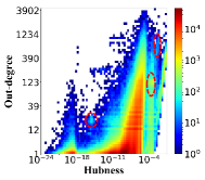
(a) Out-degree vs. Hubness

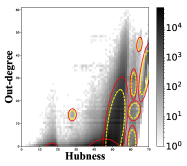
(b) Results from EagleMine.

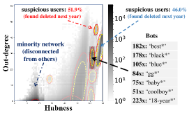
(c) Interesting and suspicious clusters.

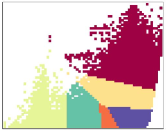
(d) X-means

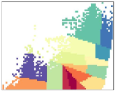
(e) G-means

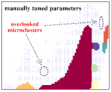
(f) DBSCAN

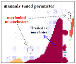
(g) STING

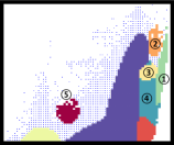
(h) Our proposed EagleMine

Figure 1: Our proposed EagleMine achieves effective results on microblog Sina Weibo data. (a) the histogram plot in heat map. (b) the summarization of EagleMine with truncated distributions. (c) suspicious users deleted from the Sina Weibo website, bots with common username prefixes, and an isolated network found by EagleMine. 182x:“best*” indicates that 182 bots have common username prefix “best” in the cluster. (d)-(h) are separately the clustering results of the baselines and EagleMine. The blue scatter points in (f)-(h) denote individual outliers. Even with extensive manual work to tune parameters, DBSCAN and STING still overlook two low-density micro-clusters (dashed circles) which are easily spotted by human vision and our EagleMine, since the fixed density threshold. Moreover, STING fails to separate three different clusters (red) on the right side of the major cluster.

2 Related work

For the Gaussian clusters, K-means, X-means[3], G-means[4], and BIRCH[5] (which is suitable for spherical clusters) algorithms suffer from being sensitive to outliers. Density based methods, such as DBSCAN[6] and OPTICS[7] are noise-resistant and can detect clusters of arbitrary shape and data distribution, while the clustering performance relies on density threshold for DBSCAN, and also for OPTICS to derive clusters from reachability-plot. RIC[8] enhances other clustering algorithms as a framework, using minimum description language as goodness criterion to select fitting distributions and separate noise. STING[9] hierarchically merges grids in lower layers to find clusters with a given density threshold. Clustering algorithms[10] derived from the watershed transformation[11], treat pixel region between watersheds as one cluster, and only focus on the final results and ignores the hierarchical structure of clusters. Community detection algorithms[12], modularity-driven clustering, and cut-based methods[13] usually cannot handle large graphs with million nodes or fail to provide intuitive and interpretable result when applying to graph clustering.

Table 1: Comparison between EagleMine and other related algorithms (DBD $=$ Dense block detection).

	X-means [3]	G-means [4]	DBSCAN [6]	BIRCH [5]	STING [9]	RIC [8]	DBD [14, 15]	EagleMine
parameter free	✓	✓				✓	✓	✓
non-spherical cluster		✓	✓		✓	✓	?	✓
anomaly detection			✓		✓	✓	✓	✓
summarization				✓	✓	✓		✓
linear in #nodes				✓	✓			✓

Supported by human vision theory, including visual saliency, color sensitive, depth perception and attention of vision system[16], visualization techniques[17, 18] and HCI tools help to get insight into data[19, 20]. Scagnostic[19, 21] diagnoses the anomalies from the plots of scattered points. [22] improves the detection by statistical features derived from graph-theoretic measures. Net-Ray[1] visualizes and mines adjacency matrices and scatter plots of a large graph, and discovers some interesting patterns. In terms of anomaly detection of the graph, [23, 24] find communities and suspicious clusters in graph with spectral-subspace plots. SpokEn[23] considers the “eigenspokes” pattern on EE-plot produced by pairs of eigenvectors of graphs, and is later generalized for fraud detection. As more recent works, dense subgraph and subtensor have been proposed to detect anomaly patterns and suspicious behavior[25, 26, 14]. Fraudar[14] proposes a densest subgraph-detection method that incorporates the suspiciousness of nodes and edges during optimization.

EagleMine differs from majority of above methods as summarized in Table 1. Our proposed method EagleMine is the only one that matches all specifications.

3 Proposed Model

First, let a graph $\mathcal{G}=(\boldsymbol{V},\boldsymbol{E})$, where $\boldsymbol{V}$ is the node set $\boldsymbol{V}$ and $\boldsymbol{E}$ is the edge set. $\mathcal{G}$ can be either homogeneous, such as friendship/following relations, or bipartite as users rating restaurants. Then our problem is informally defined as follows.

Problem 1 (Informal Definition)

Given a graph $\mathcal{G}$ and characteristics of V, we want to

1. Separate the nodes sharing similar characteristics into groups.

2. Find outliers which are small groups of nodes or scattering nodes with different characteristics and deviate away from the rest, if they exist.

Optimize: the goodness-of-fit of characteristics distribution, and the consistency of human visual recognition.

In our problem, we are free to use any sort of node features (characteristics) that can better visualize large graphs for manual pattern recognition, such as degrees, spectral quantities, number of triangles and average neighbor degree etc. To visualize feature similarity, we bucketize feature values and construct histogram by mapping nodes into corresponding histogram cells. The grid width can be selected by the approaches  in [27]. Thus nodes with similar characteristics form dense clusters of cells, which facilitates finding node groups.

More generally, each graph node can be associated with $k$ features, and nodes are located into the cells of a $k$-dimensional histogram $\mathcal{H}$. $k$ can be more than 2 even though it is not easy to visualize a high-dimensional histogram. In our work, we introduce EagleMine in a two-dimensional (2D) histogram for simplicity, which is easy to extend to the high-dimensional case.

Therefore, to separate nodes into groups and find outliers, our summarization model consists of

• Configurable vocabulary: distributions for describing dense clusters of histogram cells.

• Parameters: vocabulary term (distribution type) and parameter configuration of the distributions used for describing a cluster, and number of samples i.e. nodes in each cluster.

The configurable vocabulary can include all suitable distributions, such as Uniform, Gaussian, Laplace, and exponential distributions.

4 Our proposed method

Our method is guided by the traits of human vision and cognitive system as follows:

Trait 1

Human vision usually detects connected components, which can be rapidly recognized by eyes despite substantial appearance variation[28, 29].

This insight helps us to identify different connected and dense regions in the histogram as candidate clusters and makes refinement for smoothing.

Trait 2

Top-to-bottom recognition and hierarchical segmentation[30]. Humans organize basic elements (e.g. words, shapes, visual-areas) into higher-order groupings to generate and represent complex hierarchical structures in human cognition and visual-spatial domains.

This trait suggests organizing and exploring node groups based on a hierarchy, or tree structure, as we will do.

4.1 Water-level tree

First, let histogram $\mathcal{H}=\{h_{i,j}\,|\,i\in[1,n_{r}];j\in[1,n_{c}]\}$, where $i$, $j$ are row and column index of histogram grids respectively, and height $h_{i,j}$ is the number of nodes in the grid $(i,j)$. We name a connected region formed by non-empty grids ($h>0$) as an island, and the regions formed by empty grids as water area. Assume that we can flood island areas which makes grids with $h_{i,j}<r$ to be underwater, i.e. setting $h_{i,j}=0$, where $r$ is a water level. Then we call the resulting islands as the islands in the condition of water level $r$.

To organize all found islands during the flooding of different water-levels for histogram $\mathcal{H}$, we propose to construct a water-level tree $\mathcal{T}$. The nodes represent islands and the edges denote the relationship that child islands come from the parent island owing to the water flooding. Thus, the root of $\mathcal{T}$ corresponds water-level zero, while moving towards the leaves, the nodes are at a higher water-level of flooding.

In fact, the islands are candidate clusters as Trait 1. The flooding process intuitively reflects how human eyes hierarchically capture different objects from the color histogram $\mathcal{H}$ as Trait 2 (see Figure1(a)), where the gradient colors depict clusters at different water-levels.

The WaterLevelTree algorithm is shown in Algorithm 1. We start from the root with all non-empty grids. Rising the water-level by threshold $r$ represents scanning different density of grids. Due to the power-law-like distribution of grid heights, we use the logarithm of heights. The water-level increases from $r=0$ to $\log h_{max}$ with a fixed step size $s$, where $h_{max}=\max{\mathcal{H}}$. For smoothing the islands at each eater-level we use binary opening ($\circ$), a basic workhorse of mathematical morphology, to remove small objects (noise) from the foreground of the histogram and also separate weakly-connected parts with a specific structure element. Afterwards, we link each island at current level $r$ to its parent at level $r-1$ of the tree (see Figure2(a)). Finally, when $r=\log h_{max}$, very small grids may connect to the tree $\mathcal{T}$.

Algorithm 1 WaterLevelTree Algorithm

1:histogram $\mathcal{H}$.

2:Water-level tree $\mathcal{T}$ of islands.

3:$\mathcal{T}=$ non-empty grid set in $\mathcal{H}$ as root.

4:for water level $r=0$ to $\log{h_{max}}$ by step $s$ do

5:     $\mathcal{H}^{r}=$ assign $h_{i,j}\in\mathcal{H}$ to zero if $\log h_{i,j}<r$.

6:     $\mathcal{H}^{r}=\mathcal{H}^{r}\circ$ E. $\triangleright$ binary opening smooth.

7:     islands $\Theta^{r}=$ connected regions in $\mathcal{H}^{r}$.

8:     link each island in $\Theta^{r}$ to their parents in $\mathcal{T}$.

9:end for

10:Contract $\mathcal{T}$ by iteratively removing the single-child islands and linking its children to parent.

11:Prune $\mathcal{T}$ heuristically to remove noise islands.

12:Expand island $\theta\in\Theta$.

13:return $\mathcal{T}$

The current tree $\mathcal{T}$ may contain many nodes with only one child, meaning no actual new islands appear, which leads to many redundant nodes due to the increasing step $s$ of water-level. Therefore, we propose to use the following three steps to post-process the tree as refinement: contract, prune and expand.

Contract: We search the tree using depth-first search (DFS), and if a single-child node is found, we remove it and link its children to its parent. In the sequel, all single-child nodes will be contracted to their parents. This is shown in Figure 2(a), where the dashed lines with arrows depict that the single-child’s children are linked to its parent.

Prune: The purpose of pruning is to smooth an island which has noise peaks on top of the island due to fluctuations of grid heights. As the example at bottom right of Figure2(b) shown, the island $\theta$ is at water-level $r$. When water-level rises to $r^{\prime}$, three small peaks as noise islands connect to their parent $\theta$, so they are needed to be removed for smoothing. Thus, with a breadth-first search (BFS), we prune such child branches (including the children’s descendants) according to the heuristic rule that the total area of child islands is less than half of their parent node (see ① and ② in Figure2(b)).

Expand: For the sake of fitting an island with a vocabulary term, we try to include additional surrounding grids to avoid over-fitting in parameter learning. So we expand each island with its neighboring grids under the water, and iteratively absorb outward non-empty neighbors of each island until overlapping with other islands， or doubling the area of the original island. The expansion results are illustrated with shadowed rings in Figure2(b) (see ③).

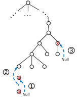
(a) Tree contract

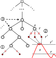
(b) Tree prune and node expand

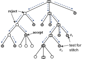
(c) Statistical hypothesis Test and optimal islands search

Figure 2: Key steps in proposed algorithms.

It is worth mentioning that in the watershed[11, 10] formalization, the non-empty areas of $\mathcal{H}$ are defined as catch basins for clustering purpose, and watersheds form the boundaries between clusters. These clusters actually correspond to the leaf islands in our water-level tree. However, EagleMine builds the whole hierarchy of islands at different water-levels. We shall see later that EagleMine searches the tree to find a better combination of clusters with hypothesis test and describes the results with vocabulary rather than only keeping leaf islands.

Another tree-based clustering algorithm STING[9] builds a multi-resolution tree for the histogram grids as an index for quick querying. The clusters were directly achieved by querying the tree-like index with density threshold $c$ as a parameter, while those clusters are actually the islands in the same level of water-level tree.

4.2 Describing islands

In the model, we define a configurable vocabulary for describing islands, which is flexible to include any user-defined distributions. As we know, many features of a graph, such as node degrees, $k$-cores, and triangles, typically follow power-law distributions, which makes some grids along the histogram boundary have the highest density (see the bottom region of Figure1(a)). Such an island can be described with a Gaussian distribution truncated at the boundary. Moreover, the truncated normal distribution is powerful enough to fit various sizes and shapes of islands, e.g. lines, circles, ellipses, truncated ellipses. Moreover, grids in histogram $\mathcal{H}$ are discrete units, so we propose to select $digitized$, $truncated$ and $multivariate$ Gaussian distribution (DTM Gaussian for short) as one of the configurable vocabulary. The DTM Gaussian distribution is defined as:

Definition 1 (DTM Gaussian distribution)

The probability function of digitized, truncated, and multivariate Gaussian is

$$P(g;\boldsymbol{\mu,\Sigma},\boldsymbol{a},\boldsymbol{b})=\int\!\!\cdots\!\!\int_{g}\psi(\boldsymbol{x};\boldsymbol{\mu,\Sigma},\boldsymbol{a},\boldsymbol{b})d\boldsymbol{x}$$

where $g$ is the grid for digitization in histogram, and the probability is an integral over hypercube $g$.

where $\psi(\boldsymbol{x};\boldsymbol{\mu,\Sigma},\boldsymbol{a},\boldsymbol{b})$ is a 2-dimensional truncated normal distribution with the mean $\boldsymbol{\mu}$, non-singular covariance matrix $\boldsymbol{\Sigma}$, and truncated at $\boldsymbol{a}=[0,0]^{T}$, $\boldsymbol{b}=[+\infty,+\infty]^{T}$ for lower and upper bound respectively.

In addition, we choose the overlapped DTM Gaussian distributions mixed with equal-weight as another vocabulary term to capture the skewed triangle-like island as shown in Figure1(a). In our data study, this triangle-like island exists in many different histogram plots, and it contains the majority of graph nodes. Taking the user-retweet-message bipartite graph as an example, Figure 1(a) depicts users’ distribution over out-degree and hubness (the first left singular vector). The power-law makes the density decrease along the vertical axis, and users with the same degree show normal distribution horizontally due to retweeting various types of messages with different hubness.

Our model can include any predefined distributions n vocabulary. We can use distribution-free statistical hypothesis test, like Pearson’s $\chi^{2}$ test, or other heuristic-based approaches (as shown later) to decide the optimal distribution for each island in practice. With the above vocabulary, we use maximum likelihood estimation to learn the parameter configuration for each term. To learn the number of samples $N$, we minimize the total expectation error of all grids in an island: $\sum_{g}\left\lVert N\cdot P(g;\cdot)-h\right\rVert$. We can choose the size of training data as $N$ directly since this optimizes log-likelihood.

4.3 EagleMine Algorithm

The overall view of our EagleMine algorithm is described in Algorithm 2. EagleMine hierarchically detects micro-clusters in the histogram plot $\mathcal{H}$, and outputs the parameters $\boldsymbol{C}$ of vocabulary term (e.g. single or mixture of DTM Gaussian), parameter configuration, and number of samples for summarization. The key steps are shown as follows.

First, the water-level tree $\mathcal{T}$ is constructed as Algorithm 1. We then decide the configurable term $y_{\theta}$ for each node $\theta$. In particular, we choose the mixture DTM Gaussian for a node depending on two observations: 1) the majority of normal nodes located at large triangle-like dense area; 2) one of the children should inherit the mixture distribution from the parent since children are part of their parent island in lower water level of $\mathcal{T}$. Thus, we get the vocabulary term $y_{\theta}$ for each island node, which is either DTM Gaussian or its mixture.

Afterwards, we search along the tree $\mathcal{T}$ with BFS to select the optimal combination of clusters (see step 5 to 14), based on the statistical hypothesis test (Anderson-Darling test[31]). $DistributionFit(\theta,y_{\theta})$ is used to denote the process of learning parameters for term $y_{\theta}$.

Algorithm 2 EagleMine Algorithm

1:histogram $\mathcal{H}$ for node features of graph $\mathcal{G}$.

2:summarization $\boldsymbol{C}$ consisting of distribution type, fitting parameters and number of samples for each distribution.

3:$\boldsymbol{C}=\emptyset$

4:$\mathcal{T}=$ WaterLevelTree$(\mathcal{H})$

5:$Y=$ decide distribution type $y_{\theta}$ from vocabulary for each island in $\mathcal{T}$.

6:queue $\boldsymbol{Q}=$ root node of $\mathcal{T}$.

7:while  $\boldsymbol{Q}\neq\emptyset$ do $\triangleright$ breath-first search (BFS)

8:     ${\theta}\leftarrow$ dequeue of $\boldsymbol{Q}$.

9:     $c=DistributionFit(\theta,y_{\theta})$

10:     Hypothesis test $\boldsymbol{H}_{0}=$ grids of island ${\theta}$ come from distribution $c$.

11:     if $\boldsymbol{H}_{0}$ is rejected then

12:         enqueue all the children of ${\theta}$ into $\boldsymbol{Q}$

13:     else

14:         add $c$ into $\boldsymbol{C}$

15:     end if

16:end while

17:Stitch promising distributions in $\boldsymbol{C}$.

18:return summarization $\boldsymbol{C}$.

Starting from the root node of $\mathcal{T}$, for each node $\theta$ in search queue $\boldsymbol{Q}$, we fit it with $c$ in configurable vocabulary. To decide whether to continue the BFS search, we then assume the following null hypothesis:

$$\boldsymbol{H}_{0}\text{: the grids of island $\theta$ come from distribution $c$.}$$

Due to the variability of the grid-height in each island, we have tried Pearson’s $\chi^{2}$ test, BIC and AIC criteria, but the extreme heights made the test and other criteria unstable. Thus, we test an island based on its binary image, which focuses on whether the island’s shape looks like a truncated Gaussian or mixture. In performing the hypothesis test, we project the grids on the major and minor axis separately in 2D space, and we accept the null hypothesis only when $\boldsymbol{H}_{0}$ is true for both orientations. So one-dimensional Anderson-Darling test (1% significant level) is conducted on both axes, and if one of the tests is rejected, the null hypothesis will be rejected.

If $\boldsymbol{H}_{0}$ is not rejected, we stop searching the island’s children and use current parameter $c$ to describe the island $\theta$. Otherwise, we need to further explore the descendants of $\theta$. The dashed lines with an arrow in Figure2(c) demonstrate this process. The final optimal combination of islands is shown in circles with texture.

Furthermore, some tiny small islands in the results $\boldsymbol{C}$ may come from different parents (e.g.  $\theta_{1}$ and $\theta_{2}$ in Figure2(c)). In such case, those islands that are physically close to each other may potentially be summarized by one distribution from the vocabulary. Thus, we use stitch process in step 15 to merge them. In the same way, we perform Anderson-Darling test to every pair of promising islands until no more changes occur. When there are multiple pairs of islands that be merged at the same time, we heuristically choose the islands pair with the least average log-likelihood reduction after stitching:

$$(\theta_{i^{*}},\theta_{j^{*}})=\operatorname*{arg\,min}_{i,j}\frac{\mathcal{L}_{i}+\mathcal{L}_{j}-\mathcal{L}_{ij}}{\text{\#points of $\theta_{i}$ and $\theta_{j}$}}$$

where $\theta_{i}$ and $\theta_{j}$ are the pair of islands to be merged, $\mathcal{L}_{(\cdot)}$ is log-likelihood of a island, and $\mathcal{L}_{ij}$ is the log-likelihood of the merged island.

At last, the summarization $\boldsymbol{C}$ of the histogram $\mathcal{H}$ is returned. Moreover, the histogram grids with very low probability ( $<10^{-5}$) from all distributions are outliers.

Furthermore, since the only one main island fitted by mixture distribution contains the majority and normal nodes, we calculate the suspiciousness of other islands by the KL-divergence of their distributions: $\sum_{g}N_{i}\cdot\text{KL}(P_{\theta_{i}}(g)\,||\,P_{\theta_{m}}(g)),$ where $\theta_{m}$ is the main island, $P(g)$ is the probability in grid $g$, and $N_{i}$ is the number of samples from the distribution of island $\theta_{i}$.

4.4 Time complexity

Given the features associated with nodes $\boldsymbol{V}$, the time complexity for generating histogram $\mathcal{H}$ is $O(|V|)$.

Let $M$ be the number of non-empty grids in the histogram $\mathcal{H}$, and $K$ be the number of clusters. We use gradient-descent to learn parameters in $DistributionFit(\cdot)$ of EagleMine algorithm, so we assume that the number of iterations is $T$, which is related to the differences between initial and optimal objective values. Then we have:

Theorem 4.1

The time complexity of EagleMine algorithm is $O(\displaystyle\frac{\log h_{max}}{s}\cdot M+K\cdot T\cdot M)$.

• See the supplementary document.

5 Experiments

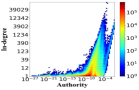
(a) In-degree    vs. Authority

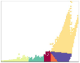
(b) X-means {6}

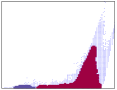
(c) sting (manual) {2}

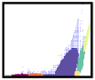
(d) EagleMine {6)}

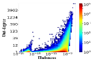
(e) Out-degree   vs. Hubness

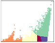
(f) X-means {5}

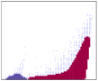
(g) sting (manual) {2}

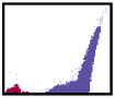
(h) EagleMine {2}

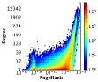
(i) Degree vs. PageRank

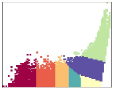
(j) X-means {5}

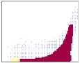
(k) DBSCAN (manual) {2}

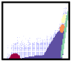
(l) EagleMine {5}

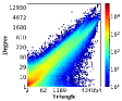
(m) Degree vs. Triangle

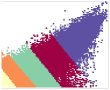
(n) X-means {5}

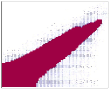
(o) DBSCAN (manual) {1}

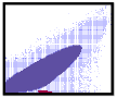
(p) EagleMine {2}

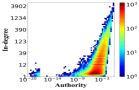
(q) In-degree    vs. Authority

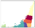
(r) X-means {7}

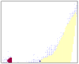
(s) sting (manual) {3}

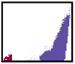
(t) EagleMine {2}

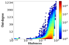
(u) Out-degree   vs. Hubness

(v) X-means {6}

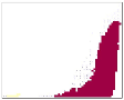
(w) DBSCAN (manual) {1}

(x) EagleMine {1}

Figure 3: Qualitative evaluation (vision-based) on real-world datasets. (a)-(d): Sina weibo data. (e)-(h): Amazon movies data. (i)-(p): Flickr friendship data (Homogeneous graph); (q)-(x): Yelp products online review. The clusters found by EagleMine agrees well with human vision. The number of clusters from each algorithm is in brackets after the algorithm name.

We design experiments to answer following questions:

1. Quantitative evaluation on real data: Does EagleMine give significant improvement in concisely summarizing the graph?

2. Qualitative evaluation (vision-based): Does EagleMine accurately detect micro-clusters that agree with human vision?

3. Anomaly detection: Does EagleMine detect suspicious patterns in real world graphs?

4. Scalability: Is EagleMine scalable with regard to the data size?

We test EagleMine on a variety of real world datasets, whose details are offered in Table 2.

Table 2: Graph datasets used in our experiments.

	# of nodes	# of edges	Content
Amazon rating[32]	(2.14M, 1.23M)	5.84M	Rate
Android[33]	(1.32M, 61.27K)	2.64M	Rate
BeerAdvocate [34]	(33.37K, 65.91K)	1.57M	Rate
Flickr[35]	(2.30M, 2.30M)	33.14M	Friendship
Yelp[36]	(686K, 85.54K)	2.68M	Rate
Youtube[37]	(3.22M, 3.22M)	9.37M	Who-follow-who
Sina weibo	(2.75M, 8.08M)	50.1M	User-retweet-msg

5.1 Q1. Quantitative Evaluation on Real Data

Envisioning the problem of clustering as a compression problem, we use Minimum Description Length (MDL) as the metric to measure the conciseness of histogram summarization. The best result $\mathcal{M}$ will minimize $L=L_{\mathcal{M}}+L_{\epsilon}$, where $L_{\mathcal{M}}$ is the length in bits of description of the model, and $L_{\epsilon}$ is the description length of differences (errors) between observed data and model expectation. For the histogram $\mathcal{H}$, denote the model expectation as $\tilde{h}$ for the number of node $h$ in grid $g$, and with the description errors that can be decoded from $L_{\epsilon}$, the original data can be accurately recovered as $h=\tilde{h}+\epsilon$. We extend Elias codes [38, 8] by encoding the sign with an extra bit, denoted as $\omega(\cdot)$. Then we encode the total description error as $L_{\epsilon}=\sum_{g}{\omega(h-\tilde{h})}$.

Therefore, the total code length of EagleMine is:

(5.1) $$L=\omega(K)+\sum_{i}^{K}(5l_{c}+\omega(N_{i}))+L_{e}$$

where $l_{c}$ is the fixed code length for floating-point number $K$ is the number of distributions used in the summary and each DTM Gaussian needs 5 free parameters. $N_{i}$ is the number of samples for distribution $i$.

We compared our summarization of micro-clusters with other clustering algorithms: X-means, G-means, DBSCAN, and EagleMine with digitized multivariate Gaussian distribution as vocabulary term, denoted as EagleMine (DM). In particular, G-means hierarchically split each cluster into two based on hypothesis test of Gaussian distribution, so we viewed it as a summarization of clusters with the Gaussian distribution. Hence, we first estimated the mean and covariance for each cluster from G-means, and then calculated MDL as equation (5.1). As for other baselines, we calculated the MDL of clustering results as[39, 8].

The parameters of baselines were set as following

1. X-means: initialized with $k$-means ($k=5$).

2. G-means: $max\_depth=5$, which meant having 16 clusters at most, to avoid too many fine-grained clusters. P-value was $0.01$ which was not sensitive.

3. DBSCAN: Eps=$1$, and used Manhattan distance. We searched MinPts from the mean of $h_{i}\in\mathcal{H}$ to the upper bound by a step of 50, and manually chose the best clusters.

The comparison of MDL is reported in Figure 4(a). We can see that EagleMine achieves the shortest description length, indicating a concise histogram summarization. On average, EagleMine reduces the MDL code length more than $42.9\%,36.4\%,17.6\%$ compared with X-means, DBSCAN, and G-means respectively. Our EagleMine also outperforms EagleMine (DM) without truncation. Therefore, EagleMine performs the best for histogram summarization with DTM Gaussian and overlapped distributions.

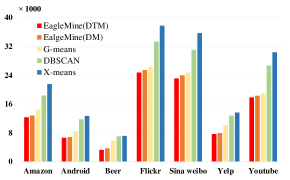
(a) MDL Quantitative Evaluation

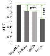
(b) AUC for suspicious users

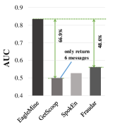
(c) AUC for suspicious messages

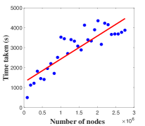
(d) EagleMine running time

Figure 4: EagleMine Performance. (a) MDL is compared on different real-world datasets. EagleMine achieves the shortest description code length, which means concise summarization, and outperforms all other baselines. (b) and (c) EagleMine has the best AUC for detecting suspicious users and messages on Sina weibo. (d) The curve blue shows the running time of EagleMine , compared to a linear function.

5.2 Q2. Qualitative evaluation (vision-based)

In this part, we visually compare the clustering results from all methods. Based on the summarization $\boldsymbol{C}$ of EagleMine, the grids can be assigned to the distribution in $\boldsymbol{C}$ and labeled as $\boldsymbol{A}$. With $\boldsymbol{A}$ and outliers, EagleMine can be compared with other clustering algorithms.

Figure3 exhibits the results of X-means, DBSCAN, STING, and EagleMine on some histograms of out-degree vs. hubness, in-degree vs. authoritativeness, degree vs. page-rank, and degree vs. triangle. Excluding outliers labeled with blue color on plots, the number of clusters found by each method is listed in the bracket after corresponding algorithm name. From the figures, it will be naturally expected that grids with similar color (density) and near location should be as one cluster, and denser parts should be covered as many as possible. The results show that X-means produces a number of poor quality clusters, as it divides the triangle-like island into pieces, which should be as one cluster, into different spherical b locks in a way inconsistent with vision-based judgment.

Although manually tuned DBSCAN captures dense regions, it overlooks some important micro-clusters as Figure1(h) shown. Moreover, the performance of DBSCAN relies on extensive manual work to pick a good result. Our EagleMine gives the best results for mining clusters, which is better than density-based clustering methods, and also captures some small micro-clusters and outliers, coinciding with human visual intuition. Moreover, EagleMine provides cluster descriptions using distributions, which summarizes data with statistical characteristics. Of course, EagleMine does not yield these micro-clusters or outliers if the features under-study do not show clustering structure as in Figure3(x).

The STING algorithm is equivalent to DBSCAN in an extreme condition[9]. It hence achieves very similar result to DBSCAN (see Figure1(g)). Besides, it does not separate the three micro-clusters and the majority cluster in red color. Therefore, our EagleMine gives better results for clustering and has more explainable results as manual recognition. It is worth noticing that some small micro-clusters captured by EagleMine are interesting patterns or suspicious groups.

5.3 Q3. Anomaly detection

In this section, we analyze the anomaly patterns in micro-clusters of Sina Weibo dataset, which is a user-retweet-message graph. The data was collected through the whole month of Nov 2013. The statistics information is listed in Table 2.

Surprisingly, we found a cluster of users who had suspicious name patterns. As Figure1(c) shows, these accounts share several prefixes, e.g. 182 usernames with prefix “best”, and 178 usernames with prefix “black”. Moreover, since those users gathered in a cluster with small covariance, they had similar out-degree $123\pm 5$ (i.e. number of retweets), and similar hubness, indicating that they retweeted the same messages, or messages with equal popularity. Based on the analysis, these users are possibly bots with synchronized behaviors.

To compare the performance for anomaly detection, we labeled these nodes, both users and messages, from the results of baselines, and sample nodes of our suspicious clusters of EagleMine considering it is impossible to label all the nodes. Our labels were based on the following rules[14]: 1 user-accounts/messages which were deleted from the online system (system operators found the suspiciousness) ; 2 users with specific login-names pattern and other suspicious signals e.g. approximately the same sign-up time, friends and followers count as discussed above; 3 messages talking about advertisement or retweeting promotion.

In total, we labeled 5,474 suspicious users and 4,890 suspicious messages. We compared with state-of-the-art fraud detection algorithms GetScoop[24], SpokEn[23], and Fraudar[14], and the results are reported in Figure 4(b) 4(c). We sorted our suspicious nodes in the descendant order of hubness or authority scores. The AUC (the area under the ROC curve) was used as the metric. The results show that EagleMine achieves more than $10\%$ improvement in suspicious user detection, and about $50\%$ improvement in suspicious message detection, which outperforms the baselines. As Figure1(h) shows, the anomalous users detected by Fraudar and SpokEn only fall in cluster ①, while EagleMine detects suspicious users from other clusters as well. Simply put, the baselines miss most of the anomalies in clusters ② and ③, while EagleMine catches them.

Finally, in Figure 1(h), we also found that the bottom left cluster consists of an isolated network, in which users retweeted different messages from those retweeted by other users out of network. In other words, users in the network did not “connect” to the outside users via messages in the bipartite graph (user-retweet-message).

5.4 Q4. Scalability

Figure 4(d) shows the near-linear scaling of EagleMine’s running time in the numbers graph nodes. Here we used Sina Weibo dataset, and subsampled the nodes to generate different size graphs.

6 Conclusion

We propose a tree-based approach EagleMine to mine and summarize all node groups in a histogram plot of a large graph. The EagleMine algorithm finds optimal clusters based on water-level tree and hypothesis test, describes them with a configurable model vocabulary, and detects some suspicious. EagleMine has desirable properties:

• Automated summarization: Our algorithm automatically summarizes a given histogram with vocabulary of distributions, inspired by human vision to find the graph node groups and outliers.

• Effectiveness: We compared EagleMine on real data with the baselines, the result shown that our detection is consistent with human vision, achieves better MDL in summarization, and has better accuracy in anomaly detection.

• Scalability: EagleMine algorithm runs near linear in the number of graph nodes.

References

- [1] U. Kang, J. Y. Lee, D. Koutra, and C. Faloutsos, “Net-ray: Visualizing and mining billion-scale graphs,” in PAKDD, 2014.
- [2] D. Koutra, D. Jin, Y. Ning, and C. Faloutsos, “Perseus: an interactive large-scale graph mining and visualization tool,” VLDB, pp. 1924–1927, 2015.
- [3] D. Pelleg, A. W. Moore et al., “X-means: Extending k-means with efficient estimation of the number of clusters.” in ICML, 2000, pp. 727–734.
- [4] G. Hamerly and C. Elkan, “Learning the k in k-means,” NIPS, p. 2003, 2004.
- [5] T. Zhang, R. Ramakrishnan, and M. Livny, “Birch: An efficient data clustering method for very large databases,” in SIGMOD, 1996, pp. 103–114.
- [6] M. Ester, H.-P. Kriegel, J. Sander, X. Xu et al., “A density-based algorithm for discovering clusters in large spatial databases with noise.” in KDD, 1996.
- [7] M. Ankerst, M. M. Breunig, H.-P. Kriegel, and J. Sander, “Optics: ordering points to identify the clustering structure,” in SIGMOD, 1999, pp. 49–60.
- [8] C. Böhm, C. Faloutsos, J.-Y. Pan, and C. Plant, “Robust information-theoretic clustering,” in SIGKDD, 2006, pp. 65–75.
- [9] W. Wang, J. Yang, R. Muntz et al., “Sting: A statistical information grid approach to spatial data mining,” in VLDB, 1997, pp. 186–195.
- [10] J. B. Roerdink and A. Meijster, “The watershed transform: Definitions, algorithms and parallelization strategies,” Fundamenta informaticae, 2000.
- [11] L. Vincent and P. Soille, “Watersheds in digital spaces: an efficient algorithm based on immersion simulations,” PAMI, pp. 583–598, 1991.
- [12] A. Lancichinetti and S. Fortunato, “Community detection algorithms: a comparative analysis,” Physical review E, p. 056117, 2009.
- [13] S. E. Schaeffer, “Graph clustering,” Computer science review, pp. 27–64, 2007.
- [14] B. Hooi, H. A. Song, A. Beutel, N. Shah, K. Shin, and C. Faloutsos, “Fraudar: Bounding graph fraud in the face of camouflage,” in SIGKDD, 2016, pp. 895–904.
- [15] J. Pei, D. Jiang, and A. Zhang, “On mining cross-graph quasi-cliques,” in SIGKDDD, 2005, pp. 228–238.
- [16] M. Heynckes, “The predictive vs. the simulating brain: A literature review on the mechanisms behind mimicry,” Maastricht Student Journal of Psychology and Neuroscience, 2016.
- [17] C. Ware, “Color sequences for univariate maps: theory, experiments and principles,” IEEE Computer Graphics and Applications, pp. 41–49, Sept 1988.
- [18] M. Borkin, K. Gajos, A. Peters, D. Mitsouras, S. Melchionna, F. Rybicki, C. Feldman, and H. Pfister, “Evaluation of artery visualizations for heart disease diagnosis,” IEEE Trans. on Visualization and Computer Graphics, pp. 2479–2488, 2011.
- [19] J. W. Tukey and P. A. Tukey, “Computer graphics and exploratory data analysis: An introduction,” Nat Computer Graphics Association, 1985.
- [20] L. Akoglu, D. H. Chau, U. Kang, D. Koutra, and C. Faloutsos, “Opavion: Mining and visualization in large graphs,” in SIGMOD, 2012, pp. 717–720.
- [21] A. Buja and P. A. Tukey, Computing and graphics in statistics. Springer-Verlag New York, Inc., 1992.
- [22] L. Wilkinson, A. Anand, and R. L. Grossman, “Graph-theoretic scagnostics.” in INFOVIS, 2005.
- [23] B. A. Prakash, A. Sridharan, M. Seshadri, S. Machiraju, and C. Faloutsos, “Eigenspokes: Surprising patterns and scalable community chipping in large graphs,” in PAKDD, 2010, pp. 435–448.
- [24] M. Jiang, P. Cui, A. Beutel, C. Faloutsos, and S. Yang, “Inferring strange behavior from connectivity pattern in social networks,” in PAKDD, 2014, pp. 126–138.
- [25] R. Kumar, J. Novak, and A. Tomkins, “Structure and evolution of online social networks,” in Link mining: models, algorithms, and applications. Springer, 2010.
- [26] J. Chen and Y. Saad, “Dense subgraph extraction with application to community detection,” IEEE Trans. on knowledge and Data Engineering, pp. 1216–1230, 2010.
- [27] L. Wasserman, All of Nonparametric Statistics (Springer Texts in Statistics). Springer-Verlag New York, Inc., 2006.
- [28] J. J. DiCarlo, D. Zoccolan, and N. C. Rust, “How does the brain solve visual object recognition?” Neuron, pp. 415 – 434, 2012.
- [29] X.-M. Liu, R. Ji, C. Wang, W. Liu, B. Zhong, and T. S. Huang, “Understanding image structure via hierarchical shape parsing,” in CVPR, 2015.
- [30] P. Arbelaez, M. Maire, C. Fowlkes, and J. Malik, “Contour detection and hierarchical image segmentation,” PAMI, pp. 898–916, 2011.
- [31] M. A. Stephens, “Edf statistics for goodness of fit and some comparisons,” Journal of the American statistical Association, pp. 730–737, 1974.
- [32] “Amazon ratings network dataset,” http://konect.uni-koblenz.de/networks/amazon-ratings.
- [33] J. McAuley, R. Pandey, and J. Leskovec, “Inferring networks of substitutable and complementary products,” in KDD, 2015, pp. 785–794.
- [34] J. J. McAuley and J. Leskovec, “From amateurs to connoisseurs: modeling the evolution of user expertise through online reviews,” in WWW, 2013, pp. 897–908.
- [35] J. McAuley and J. Leskovec, “Image labeling on a network: using social-network metadata for image classification,” ECCV, pp. 828–841, 2012.
- [36] “Yelp dataset challenge,” https://www.yelp.com/dataset_challenge.
- [37] A. Mislove, M. Marcon, K. P. Gummadi, P. Druschel, and B. Bhattacharjee, “Measurement and analysis of online social networks,” in SIGCOMM, 2007.
- [38] P. Elias, “Universal codeword sets and representations of the integers,” IEEE trans. on information theory, pp. 194–203, 1975.
- [39] D. Chakrabarti, S. Papadimitriou, D. S. Modha, and C. Faloutsos, “Fully automatic cross-associations,” in SIGKDD, 2004, pp. 79–88.